Abstract
The current airspace route system consists mainly of pre-defined routes with a low number of intersections to facilitate air traffic controllers to oversee the traffic. Our aim is a method to create an artificial and reliable route network based on planned or as-flown trajectories. The application possibilities of the resulting network are manifold, reaching from the assessment of new air traffic management (ATM) strategies or historical data to a basis for simulation systems. Trajectories are defined as sequences of common points at intersections with other trajectories. All common points of a traffic sample are clustered, and, after further optimization, the cluster centers are used as nodes in the new main-flow network. To build almost-realistic flight trajectories based on this network, additional parameters such as speed and altitude are added to the nodes and the possibility to take detours into account to avoid congested areas is introduced. As optimization criteria, the trajectory length and the structural complexity of the main-flow system are used. Based on these criteria, we develop a new cost function for the optimization process. In addition, we show how different traffic situations are covered by the network. To illustrate the capabilities of our approach, traffic is exemplarily divided into separate classes and class-dependent parameters are assigned. Applied to two real traffic scenarios, the approach was able to emulate the underlying route systems with a difference in median trajectory length of 0.2%, resp. 0.5% compared to the original routes.
1. Introduction
The route structure today is the backbone for air traffic controllers to manage regions with dense traffic. Therefore, the identification of main traffic flows and the generation of the underlying route network is an important task in building artificial but realistic future traffic samples for fast or real-time simulation environments. Those traffic samples are needed, e.g., to test free-routing strategies or the impact of eco-efficient flight trajectories. The latter results in route changes over time and takes advantage of a dynamically adapting route network. Furthermore, the approach presented here can be applied also to generate a route network for surface traffic of vehicles on airports [1].
We create a network of main flows based on current trajectories and use it as basis for a dynamically adaptable network of flow-centric routes. Here, flight trajectories are defined as a sequence of points that the observed trajectory has in common with other trajectories of the selected traffic sample instead of a sequence of turning points as, e.g., in [2], which may be individual for a route. Therefore, the points that a trajectory has in common with other trajectories are calculated (Figure 1a) and ordered depending on the distance to the corresponding flight’s origin. Close-by intersection points of different trajectories are aggregated to one representative called common point (CP). The original trajectory is then substituted by the sequence of links between these aggregated CPs (Figure 1b). The resulting trajectory is called CP trajectory.

Figure 1.
(a) Intersection points (green circles) of a trajectory (blue line) and its intersecting trajectories (red lines); (b) Resulting CP trajectory (blue line) with aggregated common points (yellow circles).
A route network is built by aggregating current or planned trajectory data to crossing points connected by links. A network’s crossing points are indicated by several streams of flights using them. Therefore, relevant points for a network are those spots, where a high number of trajectories have CPs.
The application of clustering and optimization techniques to the set of all CPs identifies these main crossing points, analyses the structure of the traffic and creates a network of typical flight routes. This is not necessarily identical to the issued route network. The crossing points are the nodes of a graph system representing the underlying flight route network.
We have shown the basic principle on how a network can be constructed from main flows in [3]. In this contribution, we introduce a new cost function that allows us to consider a route’s complexity during optimization, focus on how overload of a specific part of the network may be avoided and calculate typical class-dependent flight parameters for the CPs. Therefore, it is possible to divide the traffic in dependence on pre-defined aircraft classes such as weight vortex classes, noise, or environmental impact level. Then, typical flight heights and speeds for these aircraft classes can be determined and associated with class-dependent main flows. Since the direction of flights is not directly considered, undirected connections between cluster centers build the main flows. Opposing flights are separated vertically using different flight levels, e.g., semicircular cruising levels. To prove the feasibility of this approach, two scenarios with different traffic parameters are simulated, analyzed, and compared with focus on trajectory length, resp. similarity to the original trajectories.
The paper is structured as follows: An overview of related work and methods applied is provided in Section 2. A summary of the mathematical background is given in Section 3.1 and Section 3.2. The general approach together with all steps to build the identified main routes and flight class-dependent parameters is described in Section 3.3. Section 4 contains the simulation setup with assumptions and limitations, used metrics, traffic scenarios, and simulation parameters. The results of the simulations are presented and discussed in Section 5.
2. Status Quo
ATM research projects often use artificial flight trajectories to assess new scientific questions. For a realistic baseline, these artificial trajectories should be as closely as possible to the standard trajectories used in the observed part of the airspace.
A straight-forward approach to define a route network is to identify those parts of the airspace which are used quite often and by a higher number of aircraft. In the literature [4] this is carried out with different methods, e.g., by clustering trajectories or identifying and clustering segments of trajectories.
In the case of trajectory clustering, complete trajectories are considered, and similar ones are grouped together [5,6,7]. Therefore, it is possible to distinguish between routes with different origin or destination even in case of overlapping segments. This can be used to identify and analyze traffic flows [8] in controller support tools.
By clustering segments of trajectories, sections are determined that several trajectories have in common. These segments are the basis for an artificial route network. Therefore, turning points of flights are identified and used as waypoints [2,9]. In the case of arrival or departure routes, some segments of these routes represent links to resp. from certain directions and some are common for all routes (e.g., glide path). Reference [7] uses a two-step clustering approach and a shortest-path algorithm to optimize flight trajectories. Here, we use similar steps to create a new airspace structure as described in Section 3.3.
Especially trajectory clustering approaches rely on the selection of an appropriate similarity measure to compare trajectories or trajectory segments. Over recent years, many metrics were proposed and tested. Among the most common described in [4,10] are Euclidian, Haussdorff, and Frechet. Also usual is “Longest Common Sub-Sequence Metric (LCSS)” presented in [11]. A more recent metric called “Symmetrized Segment-Path Distance (SSPD)” was developed in [10] and applied in [5]. In this paper, we use this metric to compare the results to the as-flown trajectories.
For clustering trajectories, parts of trajectories, or waypoints an appropriate clustering algorithm must be selected. In general, clustering algorithms [12] can be assigned to different techniques such as partition or distance-based clustering, density-based clustering [9], Ref. [4,8] or hierarchical clustering such as HDBSCAN [13]. The well-known k-means algorithm and its variants [14] are distance-based clustering techniques. Widespread density-based clustering algorithms are based on DBSCAN (Density-Based Spatial Clustering of Applications with Noise) [15]. Spectral clustering [16] or the OPTICS (Ordering points to identify the clustering structure) algorithm [17] are also density-based clustering algorithms showing good results in case of data sets with varying densities. As introduced in [3], we use a DBSCAN to cluster intersections of trajectories instead of trajectories or segments thereof.
3. Materials and Methods
Here, we use the DBSCAN algorithm [15] for clustering and as path finding algorithm [18] to optimize the trajectories as described below in brief. To fine-tune the cluster center positions of the main-flow structure, a Hill Climbing algorithm (step number 1000) with a Gaussian distribution (mean 0, variance 1) for x and y coordinates of the cluster centers is applied.
3.1. Clustering Algorithm DBSCAN
The DBSCAN algorithm [8,10,15,19] is a density-based algorithm, which forms clusters based on the distribution of data in space. It groups together data points that are close to each other in relation to a given distance parameter ε. A data point is defined as element of a dense region when the number of data points with a distance less than or equal to exceeds a given minimum . A given point is a core object of a cluster, if the number of all elements q within distance of point is greater than or equal to . If a point of this group is within the ε distance of p and both are core objects of the same cluster, is called “directly density reachable” from . A point is called “density reachable” from point if there is a chain of points with and where is directly density reachable from for all . They can be seen as elements of the transitive hull of a cluster. To create a cluster, a first element with at least points within its neighborhood is selected as start element. This cluster is expanded by adding all points in the ε neighborhood of the first element and additionally all elements inside the dense regions of these points (if existing) to the actual cluster. This procedure is then repeated with elements not yet assigned to a cluster, until all elements are examined. Elements, which have no dense region resp. cluster, are defined as noise. This algorithm can handle non-convex cluster shapes.
3.2. Pathfinding Algorithm
The algorithm [18] is a generalization of the Dijkstra algorithm. This pathfinding algorithm uses problem dependent information to estimate path costs. It operates on a weighted graph where the sum of costs (here the edge length) counted by moving through the network from a given origin to a destination is used as objective function. This algorithm tests those nodes first which seem to be most promising, e.g., because they are very close. For each possible node, the cost to reach this node from the origin plus the estimated cost to move from this node to the destination are calculated (. For , the length of the direct connection from the observed point to the destination is used as estimation. This is carried out until the destination is reached.
3.3. General Approach
This section describes how main flows are built from trajectories as well as the algorithm structure. The approach summarized in Section 3.3.1 and Section 3.3.2 is based on work presented in [3]. The algorithm is divided in four main steps, whereby pre-processing is denoted as step A (Figure 2) and the main-flow processing as steps B to D. Here, the focus is on how flight parameters are considered to determine more realistic traffic networks (Section 3.3.3).
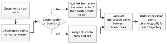
Figure 2.
Pre-processing (step A).
3.3.1. Pre-Processing
We distinguish between two different types of cluster centers: Entry/exit cluster centers located on the boundary and inner cluster centers marking traffic nodes. For cluster centers that are located on the boundary, the distance is calculated in a special way. For this, the boundary is considered to be a path with a defined start/end point. For each point on the boundary, the position is given as a percentage of the boundary length from start to this point. The distance between two points is then the difference in their position percentages. Clusters are calculated in dependence on two parameters and (Section 3.1). In a first step, entry and exit points of the observed flights are clustered separately to identify the beginnings or endings of the main-flow segments (Figure 2). For this, a DBSCAN [15] is used separately for entry and exit points to facilitate a segregation of inbound and outbound traffic. To identify the general route structure and thereby the main-flow network, the course of a flight route is the most important aspect. Noise points are assigned to the closest boundary entry/exit cluster. All flight trajectories start, resp. end at the closest identified cluster.
In the next step, the common points–points where trajectories intersect–are calculated for a pre-defined time period. For each flight, the list of common points is ordered by the distance to the flight’s origin. Thus, so-called CP trajectories consisting of links between common points are constructed. The generated traffic sample (Section 4.3) for the German airspace area has ~4 billion common points and for a part of northern Germany and the northern sea (EDYYDUTA) ~300,000.
The cluster centers calculated in the pre-processing (step A) can be interpreted as edges of the underlying route network because many trajectories from different directions use the same points.
3.3.2. Main-Flow Processing
During the main-flow processing, all common points within the airspace area are clustered with DBSCAN as density-based clustering algorithm [15]. The Euclidian distance metric is used with nautical miles [NM] as unit to measure distances. Cluster centers are calculated as representatives for groups of common points (see Figure 3).
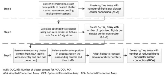
Figure 3.
Main-flow processing (steps B to D).
Resulting clusters are not necessarily convex. Common points, which DBSCAN identified as noise, are assigned to the nearest identified cluster center to ensure that each common point of the CP trajectories can be substituted by a corresponding cluster center. Due to the irregular shape of clusters, a trajectory may cross a large cluster multiple times. If non-consecutive intersections within a trajectory are associated with the same cluster (Figure 4), this may increase the trajectory length considerably because the same cluster center is revisited several times.
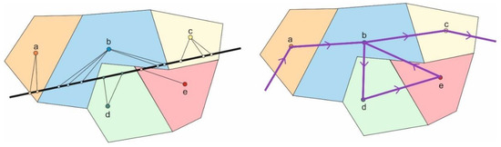
Figure 4.
Common points of original trajectory (small circles) of a trajectory (black line) and centers (larger circles) in assigned colors (left), CP trajectory after step B as sequence of cluster centers a-b-d-e-b-c in purple (right).
To build the main-flow structure, an array consisting of elements, with denoting the amount of cluster centers for the adapted main-flow network, is build (step B). In this array, the number of flights using the links between a pair of cluster centers is stored based on the selected flight sample. This Adapted Connection Array (ACA) can be interpreted as a list of all allowed connections between cluster centers and is used to calculate the main flows.
The association of common points of each trajectory with the appropriate cluster centers may still lead to routes which are longer than necessary. Therefore, the shortest route between start and end point of each flight is calculated with a path finding algorithm [18] (step C) based on the main-flow network defined by ACA. Each non-zero number at position (i, j) in the ACA is interpreted as an allowed edge between cluster center i and j. Therefore, the ACA can be used as basis for the algorithm to create the shortest possible route consisting of allowed links between cluster centers. Thus, a new connection array is determined called Optimized Connection Array (OCA).
In step D, nodes with only two connected links (one entry, one exit) are substituted by a single link between the surrounding cluster nodes based on the OCA. This procedure is not applied to cluster centers which are entries or exits of flight trajectories. In the example in Figure 5, the orange cluster center and its connections are removed and replaced by the red line.

Figure 5.
The redundant orange cluster center is removed in step D.
After step D, a point-balancing is carried out to optimize the remaining cluster center positions. This can be formalized as follows: Let be the set of cluster centers connected to a selected cluster center p. Then, the position is balanced with respect to the sum of distances to the elements for each cluster center p. This is carried out with a hill climbing algorithm using an evaluation function that takes the number of flights between point p and the connected cluster center as the length of this link into account.
The goal is to smooth the main flows used by many flights and to decrease the average length of the most frequently used main flows. Hill climbing is used to find a new position as representative of the intersection in the vicinity of the old center coordinates. Therefore, new positions are restricted to a circular area around the original position.
As last step, all CP trajectories are adapted to the reduced number of cluster centers and a new connection array is determined for the reduced main-flow system called Reduced Connection Array (RCA).
3.3.3. Calculation of Flight Parameters
To create realistic traffic samples for fast and real-time simulations, not only the positions of the network nodes are important but speed and altitude likewise. Therefore, together with the position of the common points the values for speed and flight height at these positions are taken into account. While processing the position data for cluster centers of the main-flow network, average speeds, and altitudes are calculated for the centers. In addition, it is possible to calculate these values for different classes of flight types. Examples for those classes are wake vortex, noise, or eco-efficiency classes. Therefore, special characteristics of a flight class can be resembled within a flow network.
When similar common points are merged into one representative point, the same must be carried out for speeds and altitudes. To calculate the speed or altitude of cluster centers, a point’s distance to the calculated cluster center is considered. In the case of only two common points this is simply the average. For inner clusters with more elements the method works as follows:
Let be the set of cluster centers, ‖‖ the number of cluster centers, a selected cluster center, the distance of element of the corresponding cluster i to the cluster center and the maximum distance of cluster elements to cluster center , then the weight for cluster element is calculated as
With this, a cluster center’s speed and altitude are calculated as weighted sum of speed/altitude of the cluster elements:
Here, is the speed and the altitude of the cluster element . The calculation for the boundary clusters works similar but with the distance measure defined in Section 3.3.1.
With respect to the semicircular cruising levels, one set of speed and altitude is stored for each cluster center and direction type. Subsequently, speed values are rounded to the nearest multiple of five while altitude values are assigned the nearest flight level in steps of ten, which is allowed for the flight direction with respect to the semicircular cruising levels [20].
If flight classes shall be differentiated, average values and are determined for each class separately. When speed and altitude would have been included as parameters analogous to the position data as part of the cluster data, different main-flow networks depending on the selected flight classes would have been generated. This would be different to today’s approach where flight routes itself are the same for most flight types, e.g., flights with wake vortex classes Heavy and Medium.
4. Experimental Setup
Within this section, we provide an overview of the experimental setup, including assumptions, assessment metrics, and scenarios. Two scenarios are introduced and an overview of the simulation parameters such as used flight samples, selected airspace area, and observed flight levels are given.
4.1. Assumptions and Limitations
The target of our approach is to create a basic en-route system of route designators (cluster centers) and connecting segments similar to those used today (see e.g., aeronautical information publication (AIP), ENR 3.3 RNAV Routes). The constructed main-flow network consists of bidirectional connections between cluster centers. To separate traffic with different flight directions, semicircular cruising levels are applied to the main-flow network. This follows the definition of route designators in the AIP in which many designators use odd/even flight levels for different flight directions. Nevertheless, route designators limited to one direction also exist. The limitation to airspace above flight level 320 reduces the amount of climbing and descending traffic that could otherwise disturb the flight level system depending on flight directions. Since the main-flow network is based on as-flown traffic above flight level 320, directional restrictions are automatically transferred to it.
Each entry/exit is assigned to an appropriate entry/exit cluster. Nevertheless, it is possible that there is a considerable distance between the original entry/exit point and the assigned cluster center. It is assumed that all aircraft will fly direct to their sector entry point and will resume their normal route when exiting the sector.
Since the focus of the approach presented here lies on the creation of a route structure with characteristic crossing points, not on identifying conflicts, we neglect actual flight times when calculating the common points as intersections between flight trajectories. Therefore, the intersection points are interpreted as common points where traffic may cross rather than possible conflict zones between two aircraft. Flight levels and speeds are determined depending on flight classes.
Hence, most important are the common points between the flights’ routes. They are assumed to be similar if the distance between them is less than 0.1 NM. One representative is selected and the number of similar points kept with it.
4.2. Assessment Metrics
To evaluate the results, we have selected suitable metrics. Besides the difference in trajectory length and the number of flights a cluster center serves, the trajectory distance evaluates the closeness between the original and the resulting trajectories. In addition, the structural complexity estimates the complexity of the traffic network or the influence of a partial route to the existing structure in the case of the algorithm.
4.2.1. Trajectory Distance
The SSPD metric [10] is used to evaluate the closeness between the actual flight trajectories and the artificial routes created by the trajectory clustering process. Therefore, the minimal distances for all points of trajectory G to the segments of trajectory T (Figure 6) are calculated. The average of these values determines the Segment-Path distance. For the SSPD, this is carried out for both trajectories and the sum is averaged. With this metric the route length of the flown trajectories can be compared with the route length of the artificial trajectory.
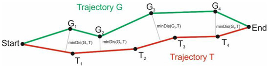
Figure 6.
Calculation of Segment-Path distance for points of trajectory to segments of trajectory . denotes the minimal distance of point to trajectory .
4.2.2. Structural Complexity of the Network
To estimate the feasibility of traffic management at a cluster center, we developed a metric for structural complexity (SC). Here, we summarize this measure in brief. For details on the structural complexity, we refer to [3]. This metric reflects the influence of a possible route system’s structure on potential controller workload [21] for a given traffic situation. Flights mostly lined up in a dominant flow—separated procedurally by altitude differences once applied—are easier to supervise than constant traffic from different directions. Therefore, the metric copes with
- Dominant flows intersected by less frequented other flows.
- Traffic from various directions with similar intensity.
- Broad variability in usage of intersection points.
We aim to assess the complexity of a possible route system rather than actual traffic flows and thereby retain some widely used aspects of ATM complexity measurement [22,23]. The angle at which two routes meet defines potential horizontal interactions. As in [23], we use 15° as lower bound, others e.g., Gianazza [24] use 20°. Route segments with an angle of −15° to 15° are handled as similar, of more than 15° to 165° as different and 165° to 180° as opposite (Figure 7). The application of semicircular cruising levels results in different flight levels for traffic with opposing flight directions. For an intersection between two route segments, the smaller angle is the determining factor. To evaluate potential horizontal interactions of a route system, we take into account a frequency for the usage of particular route segments at cluster centers.
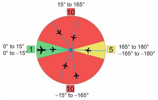
Figure 7.
Definition of similar (green), other (red) and opposite (yellow) direction between flights.
Our complexity metric is based on the angle between links and . leading to or emerging from an observed cluster center . This metric is for common points of direct routes and links from or to cluster centers. In the first case, the angle between both lines can be calculated directly as . In the second case, the common point is the cluster center and a route segment moving through this cluster center is not necessarily a straight line but may consist of any sequence of links connected to . Furthermore, not all sequences of incoming and outgoing links are used in the flight sample to the same extent.
The angle for each possible combination of in- and outgoing links is associated with a weight:
Let point be a cluster center, the set of all used link sequences of incoming and outgoing links and for this cluster center and the number of occurrences of this link sequence in all flights of the sample. The complexity factor of link sequence in combination with link sequence is defined as the average of the weights for all possible link combinations of with (see Figure 8).
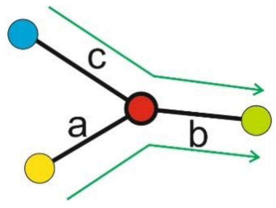
Figure 8.
Example for the combination of link sequences with , and .
The complexity value of a cluster is then defined as the sum over all complexity factors for all link combinations of multiplied by the usage frequency for each combination and divided by the sum of all usage frequencies:
The usage frequency of a link sequence is defined as for different sequences and as for the same.
The SC values for clusters are used to calculate complexity plots for the observed airspace. The airspace is overlaid with a grid with a cell size of 10 NM × 10 NM and for each cell the average of all covered cluster centers is calculated. A cell’s color ranges in ten grades from bright green to dark red and represents a cell’s average complexity within the plot.
4.2.3. Algorithm with Structural Complexity
The efficiency of a trajectory and therefore the length is one of the main concerns, especially with respect to fuel burn and related ecological aspects. Nevertheless, efficiency cannot be seen as a self-contained factor but in correlation with safety. To include safety aspects into the evaluation function of the algorithm and enable a more realistic traffic network, this function (see Section 3.2) is extended. A factor related to the ability of controllers to ensure safety is introduced. Because it is easier to monitor aircraft following nearly the same flight route or at least do not cross the flight routes of other aircraft, a route specific complexity value is added to the evaluation function. The resulting algorithm is then denoted with . This is an adaption of the structural complexity metric presented in Section 4.2.2. The target is to reduce the number of crossings for each cluster center, generate possible alternative routes and bypasses in case of heavy traffic, and thereby decrease a cluster’s structural complexity.
The partial route created by is defined as a sequence of cluster centers . For each cluster center , a list with all used link sequences moving through this cluster center is determined as in Section 4.2.2. Similar to Equation (5), a weight function is defined, leading to as complexity factor for a link sequence combination (cp. Figure 8). Subtracting 1 to ensure that only segment combinations with an angle greater than 15° influence the complexity value of a cluster center. This is according to the assumption that aircraft following each other can be handled easier than crossing routes. The complexity value for a cluster center is then defined as:
The number of cluster centers with a non-zero complexity value is denoted with . Then the evaluation value of is:
The definition of avoids a route with a higher number of cluster centers having a complexity value of zero has a better evaluation value than a shorter route with the same amount of non-zero cluster centers. To prevent changes of a cluster’s evaluation solely depending on the actual number of optimized trajectories, no usage frequency (cp. Section 4.2.2) is used in Equation (7). Otherwise would be very high if assesses a new flight whose segments introduce e.g., a 90° angle at and the existing segments in are used by a low number of flights only. would be lower if would be used by a high number of flights because a new crossing would have less influence on the traffic situation at this node.
For the evaluation function of not is added. Instead, an influence value that rates the influence of on the partial main-flow network resulting from the already optimized trajectories is considered.
Because the optimized trajectory is calculated stepwise for each adapted trajectory with , the SC values of the cluster centers included in OCA do not exist at the beginning. While optimizing trajectories one after another, the link sequences of the cluster centers are continuously extended. The sequences of already optimized trajectories are stored in an intermediate sequence array OCA*. For OCA*, the sum of complexity values of all used cluster centers with and without the partial route are calculated. The influence value is then the difference between the SC value of the main-flow system based on all optimized trajectories so far and after adding the partial route to this main-flow system. With this adaption the cost function defined in Section 3.2 can be extended to
4.3. Scenario Description and Simulation Parameters
The goal of these samples is to investigate how close a main-flow network created with the presented approach reflects the as-flown trajectories and to evaluate the influence of the optimization on a network’s structural complexity. As sample areas, the German airspace boundary (Scenario 1) and the EDYYDUTA area (Scenario 2) were selected together with appropriate traffic samples (Figure 9). EDYYDUTA includes airspace areas over the northern sea with less traffic. Both samples consist of a set of flight trajectories based on real traffic of 12 July 2012, selected from DDR2 data of EUROCONTROL [25] and restricted to flight level 320 and above. It is obvious that the trajectories of the real traffic sample are often very similar, leading to intersections which are very close to each other. However, they do not adhere in general to the published route structure. Instead, many direct routings can be identified.
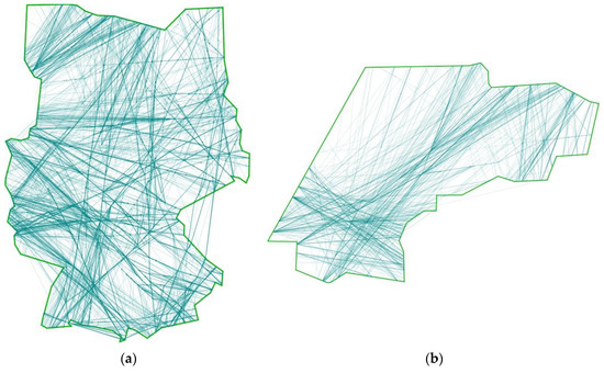
Figure 9.
German airspace boundary (a) and EDYYDUTA (b) with flown trajectories as turquoise lines. The darker the color the more flights use the corresponding part of the airspace.
In addition, the real traffic samples enable us to consider flight specific behavior such as used flight levels and speeds. The wake vortex categories Heavy, Medium and Light are used to assess and demonstrate the possibilities to calculate flight class-dependent standard speeds and altitudes for the cluster centers, resp. network nodes. Therefore, the CP trajectories created for the flights of the original traffic sample receive flight category specific speeds and altitudes.
Besides main-flow networks that allow for traffic routes as closely to the originally flown traffic as possible, the cost function of the algorithm has been extended with a structural complexity factor to evaluate the possibility of restricting more traffic to main flows. To facilitate the comparison between both variants the same simulation parameters were used.
4.4. Simulation Parameters
Several parameters must be defined for the simulations, especially for the DBSCAN algorithm. Table 1 shows the DBSCAN parameters in NM and (Section 3.2) selected to cluster the common points and the entry and exit points on the boundary for both scenarios and variants. Entries and exits were clustered separately, but with the same parameter set.

Table 1.
Parameter sets for the DBSCAN algorithm.
To select the parameter for a given value a so-called sorted k-dist graph has been used [15]. K-dist assigns to each common point the distance to its k-nearest neighbor. This is the distance necessary to include k elements in the surrounding circle of the considered intersection.
Based on this graph, several clustering tests with different values of k and associated ε in the range of the lower half of the increasing part of the k-dist curve were carried out. To construct a route network for a dense traffic distribution on defined routes where the intersections tend to agglomerate, the value must be high enough (and the resulting ε low) to identify cluster centers.
5. Results
The results for both traffic samples (Section 4.4) focus on the creation of main flows representing the general traffic streams and the identification of necessary crossways. This analysis is supplemented by a short overview of the computational efficiency for the different steps of this approach. The similarity of adapted flight trajectories to the original trajectories measured with the SSPD metric and structural complexity are the most important characteristic of this research. In addition, the length of the trajectories and typical values for speed and flight level at the identified cluster centers, respectively main-flow crossing points of the resulting network are presented.
5.1. Computational Efficiency
The computational efficiency in relation to the amount of handled data is an important factor and often a trade-off between accuracy and efficiency. To increase efficiency, we reduce the amount of common point data and the search space of the DBSCAN algorithm. Common points with a distance between them of less than 0.1 NM were defined as equal (Section 3.1). As a result, the number of possible cluster elements decreases considerably in comparison to the original number of calculated common points.
To create the ε-neighborhood for the DBSCAN algorithm, the search space is restricted to the surrounding airspace in dependence on the position of the observed cluster element. For this, the observation area is overlaid with a grid with cell size and the search space is then restricted to the cluster element’s and the adjacent cells. With these adaptions, the computation time for the DBSCAN itself (step B, Section 3.3.2) decreased considerably while the time needed for pre-processing the common points (step A) increased for higher flight numbers (Table 2).
Table 2.
Computation times in seconds for the process steps A to D (Section 3.3.1 and Section 3.3.2).
The computation time for step C depends strongly on the number of cluster centers and the connecting links, because the algorithm uses the existing links between cluster centers as possible parts of the new trajectory. Furthermore, the number of optimized trajectories influences the computation time. For step C, where an algorithm calculates the shortest route, each trajectory part between a selected pair of origin and destination point is determined only once. This optimized trajectory part is assigned to all trajectories with the same pair. This is not possible when the advanced algorithm is applied since the evaluation value of a route depends on the already optimized trajectories. This leads to a considerably higher simulation time for step Cadv. Step D includes the point-balancing functionality which as well works on each identified cluster element.
As hardware a workstation with an Intel® Xeon® E5-2186G 3.8 GHz processor (6 cores), 64 GB Ram, and Windows 10 as operating system was used. The algorithms were implemented in Java.
5.2. Main-Flow Network
Here, the goal is to emulate the real flight route system as close as possible, independently of the number of necessary cluster centers. Table 3 shows the general results for both scenarios where the cost function of the algorithm is solely based on the length of the trajectory. The numbers of common points are very high due to the high number of flights and the dissection of trajectories into segments, which are all tested for common points separately. Furthermore, several different flights use identical trajectory segments and thus intersections (start and end point) of these segments are identified as common points. As a side effect, the number of different common points is very low compared to their total number. For Scenario 2, the number of common points is considerably lower than for Scenario 1 due to the lower number of flights, but the percentage of different common points is higher for Scenario 2 (7.7%) than for Scenario 1 (1.3%). This may be caused by the less dense traffic on different routes particularly in the northern sea leading to fewer intersections at the same or a similar position.
Table 3.
Cluster structure.
The number of cluster centers is reduced by 50%, resp. 58% from adapted (step B) to reduced main-flow network (step D) for Scenario 1, resp. 2. The percentage of noise is very low for Scenario 1. Figure 10 shows the cluster elements for each cluster in an assigned color for both scenarios. The main traffic streams of Figure 9 are easily recognized. Taking the high number of common points into account it can be concluded that most flights used the main routes. This would reduce the number of common points in areas with less dense traffic and therefore the chance for the creation of a cluster center.
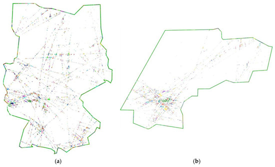
Figure 10.
Cluster elements (small dots) for Scenario 1 (a) and 2 (b) without noise. Each color marks a cluster.
Figure 10 shows the cluster elements, i.e., common points assigned to cluster centers in step B and not identified as noise. Most clusters are small with a high number of (nearly identical) elements. Comparing Figure 9b to Figure 10b shows that the north-west region has a very low number of clusters. In turn, many intersections in this area are marked as noise. This is not the case for Scenario 1 due to the dense traffic and the extensively used route system. The reduced main-flow networks presented in Figure 11 follow pre-defined flight routes and this leads to hot spots for common points, which can be easily identified. It is clearly visible that the main flows are very close to the underlying traffic for both scenarios (cp. Figure 9).
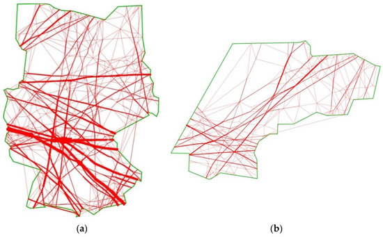
Figure 11.
Reduced main-flow system for Scenario 1 (a) and Scenario 2 (b). Line thickness reflects the number of flights using a link.
Entry and exit points were clustered separately (Section 3.3.1). For both scenarios, the minority of entry/exit points are combined points belonging to both groups (Table 4). This underpins the advantage of handling these points separately, especially with the creation of artificial traffic samples based on the main-flow network in mind. Furthermore, dividing the entry/exit points into separate groups ensures a more homogenous flow of traffic, which can be easier supervised by airspace controllers.
Table 4.
Number of entry and exit clusters.
Table 5 shows results for both scenarios for the reduced main-flow network. For both scenarios, the SSPD values are very low and the interquartile range between quartile 1 and 3 is only 2.4 in both cases. The higher median value for Scenario 2 is caused by the lower number of cluster centers and corresponding low number of route segments, particularly in the north-west part of the observed airspace.
Table 5.
Main-flow key data for both scenarios (reduced main-flow network).
Thus, several flights were unable to maintain their short as-flown routes. The results for the SSPD metric are shown in more detail in Figure 12 and confirm that most flights have very similar routes. For these routes, the SSPD is within the interquartile range while some outliers have SSPDs outside. Especially the whiskers, which mark a distance of 1.5 times the interquartile range to the median, are very close to the first and third quartile, around a value of 7 for both scenarios.
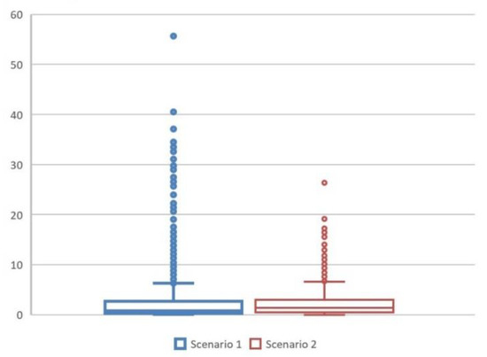
Figure 12.
Boxplot for SSPD metric for Scenario 1 (blue) and 2 (red).
Figure 13 shows two examples for higher SSPD values for Scenario 1 and 2. In both cases, the as-flown trajectory (green) is nearly a direct connection between entry and exit points. Since no direct connection between these points exists within the reduced main-flow network, the associated reduced route (in blue) has a significant difference in comparison to the original one.
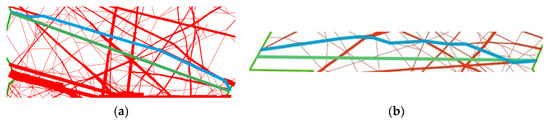
Figure 13.
Example with as-flown trajectory (green) and reduced trajectory (blue) for Scenario 1 (a, SSPD 5.7) and Scenario 2 (b, SSPD 4.0).
A comparison of the main-flow system’s median route length to the length of the original trajectories (100%) is also a metric denoting the quality of the solution. The interquartile ranges for the relative route length (Table 5) for both scenarios are small, indicating that the reduced trajectories of most flights have a comparable length.
The structural complexity SC of the main-flow networks is very low in comparison to the intersection-based SC and nearly the same for both scenarios (Figure 14 and Figure 15). The cell size is 10 NM × 10 NM and the grid color ranges from 1 (dark green) to 10 (dark red). The low values indicate a highly structured traffic network with clearly defined main flows, which are separated by different flight levels for opposing traffic streams. Only a low number of flights intersect these traffic streams from other directions. Therefore, their influence on the structural complexity is small. The high values for the intersections, especially for Scenario 2, may be caused by the individual handling of traffic by controllers, e.g., allocating a direct route in times or areas of low traffic. Since a main-flow network is based on general route structures (Section 3.3), points common for a few individual trajectories are not considered by the selected clustering algorithm. Instead, these points are marked as noise.
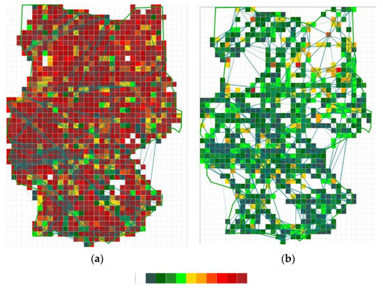
Figure 14.
Structural complexity for intersections (a) and reduced main-flow network (b) for Scenario 1.
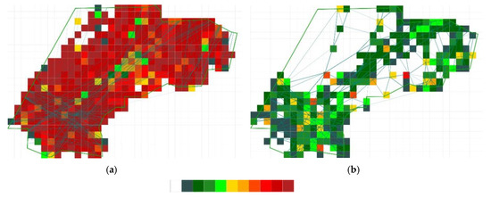
Figure 15.
Structural complexity for intersections (a) and reduced main-flow network (b) for Scenario 2.
Nevertheless, the reduced individuality of flight routes may lead to overloaded cluster centers when all flights use the prescribed flight routes. Therefore, the number of trajectories moving through a cluster center is another hint for a main-flow network’s suitability. Together with the structural complexity it can be used as an indicator for the controller workload expected when supervising these nodes. Together, they can be used as measures of safety because the number of trajectories through a cluster center and the structure of the traffic pattern influence the probability of conflicts for this point. For Scenario 1, the high number of flights compared to Scenario 2 has caused a considerably higher number of trajectories per cluster center than for Scenario 2. The interquartile range of 59 for Scenario 1 in comparison to 44 for Scenario 2 suggests a higher traffic variation among cluster centers. Therefore, it can be expected that the traffic in Scenario 1 is distributed to more cluster centers than for Scenario 2, but with a varying number of flights. This leads to an imbalance in controller workload. Nevertheless, the higher the number of cluster centers the better are the possibilities to distribute the traffic. Unfortunately, a higher amount of cluster centers tends to increase noise values, so a compromise must be found. The low number of cluster centers for Scenario 2 has led to a higher number of trajectories per cluster center as it could be expected in comparison to Scenario 1, which has more than twice the number of flights.
5.3. Flight Parameters
In addition to a general main-flow system, we have shown in Section 3.3.3 how the flight parameters altitude and speed can be reflected in such a system. Within this paper we chose the wake vortex classes Heavy, Medium and Light as an example for the distribution of flights to classes for each cluster center (Section 3.3.3). The results are displayed in Table 6 for the average flight levels and Table 7 for the average flight speeds. In addition, each identified common point was assigned to the appropriate semicircular cruising level.
Table 6.
Average flight levels for each wake vortex class and semicircular cruising level direction.
Table 7.
Average speeds for each wake vortex class and semicircular cruising level direction.
Table 6 shows that average flight levels of the flight classes are similar within a semicircular cruising level for the three classes, but as expected vary for different semicircular cruising levels. Even the small differences between the wake vortex categories imply that different flight levels are used for different categories in several cases. Aircraft with wake vortex class Light are less common in the considered scenarios due to the selected altitude range. Of the westbound flights in Scenario 2, only 63 flights belong to category Light compared to 540 in Heavy. So Light results are less reliable and presented for completeness only.
Speeds are quite different for the flight classes (Table 7). As expected, flights of wake vortex category Heavy have a higher speed than Medium flights, which are themselves on average faster than flights with wake vortex category Light. As for the flight levels, there is again a difference between east- and westbound flights, which is much more evident and may be caused by the prevailing wind direction.
5.4. Adapted Cost Function
The influence of the advanced cost function (Section 4.2.3) is assessed in this section. The idea of an additional structural complexity factor as weighted influence factor within the cost function was to reduce the number of link combinations crossing through each identified cluster center and thereby the complexity to supervise such a center. Furthermore, bypasses for nodes used by many flights are induced resulting in an increased flexibility of the resulting route network. Nevertheless, the main cost factor for the algorithm is still the trajectory length.
With (8), and therefore adopt values between 0 and 9. Thus, in Equation (9) can increase the route length of at most by nine percent. The average complexity values over all cluster centers and the proportion of average and original trajectory lengths in percent to the original trajectory have been compared for several denominator values (Figure 16). A denominator of 100 leads to a good compromise between the length of the trajectory and the reduction of the structural complexity. The “Percentage Route Length” relates the lengths of optimized trajectories created with (step C) to their original length. The average complexity value is determined in step D and therefore corresponds to the reduced trajectories. Although the results for the scenarios are on different levels in Figure 9, the structures are the same. A denominator of 50 leads in both cases to inferior results for the complexity value and the route length. A value of 10 prefers structural cluster complexity to trajectory length.
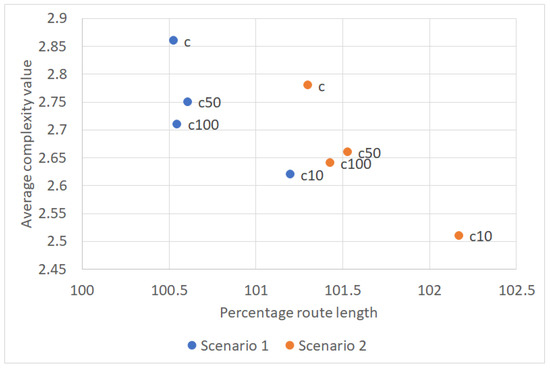
Figure 16.
Denominator tests for with (c) and denominator 10, 50, 100 (c10, c50, c100) for formula (9) for both scenarios.
Additionally, some tests were carried out were all flights between the same origin and destination got the same trajectory as the first optimized flight of this entry/exit combination (Section 5.1). In the case of , structural cluster complexity and percentage of route length increased slightly by 0.1, resp. 0.15. This indicates clearly that different trajectories are allocated to flights with the same origin and destination depending on the set of already used links between cluster centers at the time of optimization. Moreover, this leads to a higher number of flights per cluster center. Even the SSPD value increases slightly indicating that the controllers have not always assigned the same shortest route but tried to avoid e.g., crowded areas.
Table 8 compares results for and (c100) after step C for both scenarios (Section 3.3.2). The results for the structural complexity belong to step D to allow a comparison to the results of Section 5.2. For both scenarios, the route lengths with the algorithm are slightly higher and the structural complexities lower than for . Despite this, the number of links in the OCA is considerably higher for the advanced version.
Table 8.
Results for and for both scenarios. All values are medians.
With more links, necessary crossing points were able to move to a different position between two routes if many crossing links or an inappropriate crossing angle increased the cost function of . Thus, the creation of trajectories is more flexible as intended and this helps to avoid complex structures. In turn, the length of the main-flow system increases. However, SSPD and node number per optimized trajectory stay the same for Scenario 1. For Scenario 2, the trajectories for the advanced version are unable to stay as closely to the original trajectory as before. This may be caused by the considerably lower number of cluster centers and the resulting limited number of choices in case of Scenario 2.
6. Discussion
The presented approach and its processing steps allow creating a network of main flows, given as easily useable node-link network. This is proven by the comparable trajectory length and similarity to the original trajectories calculated as SSPD distance. Furthermore, the categorization of flights into classes that resemble flight specific capabilities allows for assignments of class-dependent restrictions as e.g., altitudes or speeds. As seen in Section 5.3, wake vortex categories are one possibility.
The results show that it is possible to recognize traffic structures in different traffic scenarios using common points calculated as intersections between trajectories. The median length of the trajectories for Scenario 1 and 2 in relation to the flown trajectories of 100.2% and of 100.5% as well as the low values for SSPD with 0.8 and 1.4 NM demonstrate the ability to identify and emulate the course of traffic. These good results show that most reduced trajectories are very similar to their associated as-flown trajectories and receive an appropriate reduced trajectory, while only a few trajectories must fly detours to reach their destination.
For both scenarios, the median number of cluster centers decreases considerably with the application of the algorithm in step C, where each flight is assigned to its optimized trajectory on the given adapted main-flow network. This shows that the optimization concentrates the trajectories on main routes where the workload for the affected cluster centers may increase considerably while other centers remain unused. Therefore, the distribution of traffic to the remaining cluster centers of the reduced main-flow network is important and improved with . Nevertheless, a strategy to manage the traffic might be necessary for cluster centers connected to several busy links. A first step in this direction is the assignment of different flight levels as a function of flight classes (Section 5.3).
The categorization of flights with respect to semicircular cruising levels for the clustering process enhanced the proper identification of speeds and flight levels at the identified cluster centers. The advantage of distinguishing between flight classes depends clearly on the selected class types and the scope. A classification into wake vortex categories is likewise applicable as into noise or eco-efficient categories. Whenever values depend significantly on defined classes, a division of the data is beneficial.
The structural complexity SC (Section 4.2.2) implies that the resulting route network is highly structured with clearly defined main flows. The SC of the reduced main-flow network is much lower than the SC of the as-flown traffic sample defined by the flight route intersections. Depending on the actual traffic situation, as-flown traffic may contain more flight trajectories individually assigned by controllers and thus may not reflect the original route structure entirely. Nevertheless, our main-flow network is a good approximation for the trajectories of the as-flown traffic sample as indicated by the low values for SSPD and the relative route length. On the other hand, using an optimization algorithm as A* with an evaluation function exclusively based on the route length leads to a traffic network with a reduced number of options to avoid overloaded crossing points. The adapted algorithm results in a more realistic route network with extended possibilities for detours. The results for SC are even better than for the but at the cost of a slightly increased relative route length. In conclusion, the advanced algorithm has proven to be able to find a good compromise between the structural complexity and the length of a route.
The presented approach can build a suitable main-flow network including category dependent speeds and altitudes when based on as-flown traffic samples. The use of common points between trajectories allows the main-flow network to adapt to the given traffic samples of all scenarios. The reduced main flows may be used as substitute for the underlying as-flown route network to create more realistic flight trajectories for e.g., fast time simulations instead of using the more theoretically defined flight route network. Furthermore, the resulting main-flow network may be used in situations, where traffic is re-routed—e.g., to increase eco-efficiency—or the entry and exit points of a new route are known only. Additional constraints can be transferred to the network through the categorization of the sample data and the assignment of category dependent parameters at cluster centers.
7. Conclusions
The method of clustering common points instead of complete flight trajectories described in [3] and expanded in this paper has proven to be a valid approach to identify traffic streams for different kinds of traffic samples. The presented scenarios demonstrated that the resulting traffic flows reflect the underlying traffic structure. In addition, the similarity measured with the SSPD metric is high and the median length of the resulting trajectories is comparable to the original trajectories with a difference of 0.2% for Scenario 1 and 0.5% for Scenario 2. Furthermore, the identification of main flows was possible in a short time, enabling the use in real time, e.g., to allow a time-dependent adaption of the route system to changing traffic requirements such as contrail avoidance.
Here, we have shown how the presented concept can be extended to support more realistic main-flow networks allowing detours with specific capabilities depending on aircraft categories. Exemplarily, we have shown how wake vortex categories that can be used to assign specific speeds and altitudes.
The focus of the actual approach is placed on the upper airspace in general. It can be further expanded to support different main-flow networks for particular flight types such as intercontinental traffic on higher and district traffic on lower flight levels. In this case, different combinations of origins and destinations and lengths of flight trajectories may result in different main-flow networks. To apply this method to lower flight levels or a terminal maneuvering area, considering directions in the optimization process would allow flows to separate arriving and departing traffic (as is carried out today by using standard instrument departure and standard instrument arrival routes).
Here, aircraft on opposing flight directions are separated by different flight levels as is the case with semicircular cruising levels to include the vertical component in this otherwise two-dimensional main-flow network. As discussed in more detail in [3], it is uncertain whether the removal of links with a low number of associated flights is possible without destroying the main-flow network, increasing the average trajectory length or increasing the structural complexity. The removal may lead to a reduction in the number of cluster centers and thus to a more clearly structured airspace route network, but may increase the flight number per cluster center, the risk of traffic streams from different directions and the chance for increased trajectory lengths.
Possible areas of application are the identification of route networks based on given real traffic samples to create artificial but realistic flight trajectories or the analysis of new route systems based on artificial traffic samples featuring, e.g., free-routing or contrail avoidance. Furthermore, a dynamic adaption of a route system is possible based on planned traffic data for certain time periods over a day. Regarding new requirements on trajectory planning such as eco-efficiency criteria, the presented method allows the identification of a hidden general structure which can then be re-used.
Our future work will focus on how to build more realistic main-flow networks by taking possible overload situations at cluster centers into account. The time aspect will be added insofar as to integrate knowledge about time periods where a high traffic demand can be expected, and detours to avoid congested airspace areas should be considered. Besides the network-related improvements, we will apply an evolutionary algorithm to adapt the trajectories of given traffic samples in advance with respect to a changed environmental situation where particular parts of the airspace should be avoided. The resulting main-flow network can be applied to assign routes in the flight planning phase that reduces the complexity of the traffic.
Author Contributions
Conceptualization, I.G.; Methodology, I.G. and A.T.; Software, I.G.; Writing–original draft, I.G. and A.T.; Writing–review & editing, I.G. and A.T. All authors have read and agreed to the published version of the manuscript.
Funding
This research received no external funding.
Conflicts of Interest
The authors declare no conflict of interest.
References
- Schultz, M.; Olive, X.; Rosenow, J.; Fricke, H.; Alam, S. Analysis of airport ground operations based on ADS-B data. In Proceedings of the 2020 International Conference on Artificial Intelligence and Data Analytics for Air Transportation (AIDA-AT), Singapore, 3–4 February 2020. [Google Scholar] [CrossRef]
- Gariel, M.; Srivastava, A.N.; Feron, E. Trajectory Clustering and an Application to Airspace Monitoring. IEEE Trans. Intell. Transp. Syst. 2011, 12, 1511–1524. [Google Scholar] [CrossRef]
- Gerdes, I.; Temme, A.; Schultz, M. From free-route air traffic to an adapted dynamic main-flow system. Transp. Res. Part C Emerg. Technol. 2020, 115, 102633. [Google Scholar] [CrossRef]
- Yuan, G.; Sun, P.; Zhao, J.; Li, D.; Wang, C. A review of moving object trajectory clustering algorithms. Artif. Intell. Rev. 2016, 47, 123–144. [Google Scholar] [CrossRef]
- Basora, L.; Morio, J.; Mailhot, C. A Trajectory Clustering Framework to Analyse Air Traffic Flows. In Proceedings of the 7th Sesar Innovation Days, Belgrade, Serbia, 28–30 November 2017. [Google Scholar]
- Delahaye, D.; Puechmorel, S.; Alam, S.; Feron, E. Trajectory Mathematical Distance Applied to Airspace Major Flows Extraction. In Lecture Notes in Electrical Engineering, Air Traffic Management and Systems III; Springer: Cham, Switzerland, 2018; pp. 51–66. [Google Scholar]
- Marzuoli, A.; Gariel, M.; Vela, A.; Feron, E. Data-Based Modeling and Optimization of En Route Traffic. J. Guid. Control. Dyn. 2014, 37, 1930–1945. [Google Scholar] [CrossRef]
- Olive, X.; Morio, J. Trajectory clustering of air traffic flows around airports. Aerosp. Sci. Technol. 2018, 84, 776–781. [Google Scholar] [CrossRef]
- Lee, J.-G.; Han, J.; Whang, K.-Y. Trajectory clustering: A partition-and-group framework. In Proceedings of the SIGMOD’07, Beijing, China, 11–14 June 2007. [Google Scholar] [CrossRef]
- Besse, P.C.; Guillouet, B.; Loubes, J.-M.; Royer, F. Review and Perspective for Distance-Based Clustering of Vehicle Trajectories. IEEE Trans. Intell. Transp. Syst. 2016, 17, 3306–3317. [Google Scholar] [CrossRef]
- Vlachos, M.; Kollios, G.; Gunopulos, D. Discovering Similar Multidimensional Trajectories. In Proceedings of the 18th International Conference on Data Engineering, San Jose, CA, USA, 26 February–1 March 2002. [Google Scholar] [CrossRef]
- Aggarwal, C.C.; Reddy, C.K. (Eds.) Data Clustering: Algorithms and Applications. In Data Mining and Knowledge Discovery; CRC Press: Boca Raton, FL, USA; Taylor & Francis Inc.: Oxfordshire, UK, 2014; Volume 31, ISBN 978-1466558212. [Google Scholar]
- Mc Innes, L.; Healy, J. Accelerated Hierarchical Density Clustering. In Proceedings of the IEEE International Conference on Data Mining Workshops (ICDMW), New Orleans, LA, USA, 18–21 November 2017. [Google Scholar] [CrossRef]
- Mirkin, B. Mathematical Classification and Clustering; Kluwer Academic Publishers: Dordrecht, The Netherlands, 1996; ISBN 978-1-4613-0457-9. [Google Scholar]
- Ester, M.; Kriegel, H.-P.; Sander, J.; Xu, X. A Density-Based Algorithm for Discovering Clusters. In Proceedings of the KDD-96, Portland, OR, USA, 2–4 August 1996. [Google Scholar]
- Von Luxburg, U. A tutorial on spectral clustering. Stat. Comput. 2007, 17, 395–416. [Google Scholar] [CrossRef]
- Ankerst, M.; Breunig, M.; Kriegel, H.-P.; Sander, J. OPTICS: Ordering points to identify the clustering structure. In Proceedings of the ACM SIGMOD International Conference on Management of Data, Philadelphia, PA, USA, 1–3 June 1999. [Google Scholar] [CrossRef]
- Hart, P.E.; Nilsson, N.J.; Raphael, B. A Formal Basis for the Heuristic Determination of Minimum Cost Paths. IEEE Trans. Syst. Sci. Cybern. 1968, 4, 100–107. [Google Scholar] [CrossRef]
- Sheridan, K.; Puranik, T.; Mangortey, E.; Pinon, O.; Kirby, M.; Mavris, D. An Application of DBSCAN Clustering for Flight Anomaly Detection during the Approach Phase. In Proceedings of the AIAA Scitech 2020 Forum, Orlando, FL, USA, 6–10 January 2020. [Google Scholar] [CrossRef]
- ICAO. Annex 2 to the Convention on International Civil Aviation. Rules of the Air. ICAO, 10th ed.; ICAO: Montreal, QC, Canada, 2005. [Google Scholar]
- Athènes, S.; Averty, P.; Puechmorel, S.; Delahaye, D.; Collet, C. ATC complexity and controller workload: Trying to bridge the gap. In Proceedings of the International Conference on HCI in Aeronautics, Cambridge, MA, USA, 23–25 October 2002. [Google Scholar]
- Prandini, M.; Piroddi, L.; Puechmorel, S.; Brazdilova, S.L. Toward Air Traffic Complexity Assessment in New Generation Air Traffic Management Systems. IEEE Trans. Intell. Transp. Syst. 2011, 12, 809–818. [Google Scholar] [CrossRef]
- EUROCONTROL. Complexity Metrics for ANSP Benchmarking Analysis; ACE Working Group on Complexity: EUROCONTROL: Brussels, Belgium, 2006. [Google Scholar]
- Gianazza, D. Airspace configuration using air traffic complexity metrics. In Proceedings of the 7th USA/Europe Air Traffic Management R&D Seminar, Barcelona, Spain, 2–5 July 2007. [Google Scholar]
- EUROCONTROL. DDR2 Reference Manual 2.9.5; EUROCONTROL: Brussels, Belgium, 2018. [Google Scholar]


Publisher’s Note: MDPI stays neutral with regard to jurisdictional claims in published maps and institutional affiliations. |
© 2020 by the authors. Licensee MDPI, Basel, Switzerland. This article is an open access article distributed under the terms and conditions of the Creative Commons Attribution (CC BY) license (http://creativecommons.org/licenses/by/4.0/).