Using Convolutional Neural Networks to Automate Aircraft Maintenance Visual Inspection

Abstract

Convolutional Neural Networks combined with autonomous drones are increasingly seen as enablers of partially automating the aircraft maintenance visual inspection process. Such an innovative concept can have a significant impact on aircraft operations. Though supporting aircraft maintenance engineers detect and classify a wide range of defects, the time spent on inspection can significantly be reduced. Examples of defects that can be automatically detected include aircraft dents, paint defects, cracks and holes, and lightning strike damage. Additionally, this concept could also increase the accuracy of damage detection and reduce the number of aircraft inspection incidents related to human factors like fatigue and time pressure. In our previous work, we have applied a recent Convolutional Neural Network architecture known by MASK R-CNN to detect aircraft dents. MASK-RCNN was chosen because it enables the detection of multiple objects in an image while simultaneously generating a segmentation mask for each instance. The previously obtained $F_1$ and $F_2$ scores were 62.67% and 59.35%, respectively. This paper extends the previous work by applying different techniques to improve and evaluate prediction performance experimentally. The approach uses include (1) Balancing the original dataset by adding images without dents; (2) Increasing data homogeneity by focusing on wing images only; (3) Exploring the potential of three augmentation techniques in improving model performance namely flipping, rotating, and blurring; and (4) using a pre-classifier in combination with MASK R-CNN. The results show that a hybrid approach combining MASK R-CNN and augmentation techniques leads to an improved performance with an $F_1$ score of (67.50%) and $F_2$ score of (66.37%).

1. Introduction

1.1. Automated Aircraft Maintenance Inspection

Automated aircraft inspection basically aims at automating the visual inspection process normally carried out by aircraft engineers. It aims at detecting defects that are visible on the aircraft skin which are usually structural defects [1]. These defects can include dents, lightning strike damage, paint defects, fasteners defects, corrosion, and cracks, just to name a few. Automatic defect detection can be enabled by using a drone-based system that can scan the aircraft and detect/classify a wide range of defects in a very short time. Other alternatives would be using sensors in a smart hangar or at the airport apron area. Automating the visual aircraft inspection process can have a significant impact on today’s flight operations with numerous benefits including but not limited to:

• Reduction of inspection time and AOG time: The sensors either on-board a drone or in a smart hangar can quickly reach difficult places such as the flight control surfaces in both wings and the empennage. This in turn can reduce the man hours and preparation time as engineers would need heavy equipment such as cherry pickers to have more scrutiny. The inspection time can be even further reduced if the automated inspection system is able to assess the severity of the damage and the affected aircraft structure with reference to both aircraft manuals (AMM and SRM), and recommend the course of action to the engineers. Time savings on inspection time would consequently lead to reductions of up to 90% in Aircraft-On-Ground times [2].
• Reduction of safety incidents and PPE related costs: Engineers would no longer need to work at heights or expose themselves to hazardous areas e.g., in case of dangerous aircraft conditions or the presence of toxic chemicals. This would also lead to important cost savings on Personal Protective Equipment.
• Reduction of decision time: Defect detection will be much more accurate and faster compared to the current visual inspection process. For instance, it takes operators between 8 and 12 h to locate lightning strike damage using heavy equipment such as gangways and cherry-pickers. This can be reduced by 75% if an automated drone-based system is used [3]. Such time savings can free up aircraft engineers from dull tasks and make them focus on more important tasks. This is especially desired given the projected need of aircraft engineers in various regions of the world which is 769,000 for the period 2019–2038 according to a recent Boeing study [4].
• Objective damage assessment and reduction of human error: If the dataset used by the neural network is annotated by a team of experts who had to reach consensus on what is damage and what is not, then detection of defects will be much more objective. Consequently, the variability of performance assessments by different inspectors will be significantly reduced. Furthermore, human errors such as failing to detect critical damage (for instance due to fatigue or time pressure) will be prevented. This is particularly important given the recurring nature of such incidents. For instance, the Australian Transport Safety Bureau (ATSB) recently reported a serious incident in which significant damage to the horizontal stabilizer went undetected during an inspection, and was only identified 13 flights later [5]. In [1], it was also shown that the model is able to detect dents which were missed the by experts during the annotations process.
• Augmentation of Novices Skills: It takes a novice 10,000 h to become an experienced inspector. Using a decision-support system that has been trained to classify defects on a large database can significantly augment the skills of novices.

1.2. Applications/Breakthroughs of Computer Vision

Computer vision is changing the field of visual assessment in nearly every domain. This is not surprising given the rapid advances and growing popularity of the field. For instance, the error in object detection by a machine decreased from 26% in 2011 to only 3% in 2016 which is less than human error reported to be 5% [6]. The main driver behind these improvements is deep learning which had a profound impact on robotic perception following the design of AlexNet in 2012. Image classification has therefore become a relatively easy problem to solve given that enough data are available to training the deep learning model.

Computer vision has been successfully applied in combination with drones in the civil infrastructure domain. This approach allows operators to assess the condition of critical infrastructure such as bridges and dams without the need for physically being there. The main aim is to automatically convert image or video data into actionable information. Spencer et al. [7] provides a good overview of recent applications that address the problem of civil infrastructure condition assessment. The applications can be divided into two main categories. The first category is inspection and deals with identifying damage in structural components such as cracks and corrosion [8], and detecting deviations from reference images. The second category is monitoring what focuses on static measurement of strain and displacement, as well as dynamic measurement of displacement for model analysis. Shihavuddin et al. [9] developed a deep learning-based automated system which detects wind turbine blade surface damage. The researchers used faster R-CNN and achieved a mean average precision of 81.10% on four types of damage. Similarly, Reddy et al. [10] used convolutional neural networks to classify and detect various types of damage on the wind turbine blade. The accuracy achieved was 94.49% for binary classification and 90.6% for multi class classification. Makantasis et al. [11] propose an automated approach to inspect defects in tunnels using convolutional neural networks. Similarly, Protopapadakis et al. [12] present a crack detection mechanism for concrete tunnel surfaces. The robotic inspector used convolutional neutral networks and was validated in a real-world tunnel with promising results.

The applications of computer vision and deep learning in aircraft maintenance inspection remain very limited despite the impact this field is already making in other domains. Based on the literature and technology review performed by the authors, it was found that only a few researchers and organizations are working on automating aircraft visual inspection.

One of the earliest works that uses neural networks to detect aircraft defects dates back to 2017. In this work [13], the authors used dataset images of the airplane fuselage. For each image, a binary mask was created by an experienced aircraft engineer to represent defects. The authors have used a convolutional neural network that was pre-trained on ImageNet as a feature extractor. The proposed algorithm achieves about 96.37% accuracy. A key challenge faced by the authors was an imbalanced dataset which had very few defect photos. To tackle this problem, the authors used data balancing techniques to oversample the rare defect data and undersample the no-defect data.

Miranda et al. [14] use object detection to inspect airplane exterior screws with a UAV. Convolutional Neural Networks are used to characterize zones of interest and extract screws from the images. Then, computer vision algorithms are used to assess the status of each screw and detect missing and loose ones. In this work, the authors made use of GANs to generate screw patterns using a bipartite approach.

Miranda et al. [15] point out the challenge of detecting rare classes of defects given the extreme imbalance of defect datasets. For instance, there is an unequal distribution between different classes of defects. Thus, the rarest and most valuable defect samples represent few elements among thousands of annotated objects. To address this problem, the authors propose a hybrid approach which combines classic deep learning models and few-shot learning approaches such as matching network and prototypical network which can learn from a few samples. In [16], the authors extend this work by questioning the interface between models in such a hybrid architecture. It was shown that, by carefully selecting the data from the well-represented class when using few-shot learning techniques, it is possible to enhance the previously proposed solution.

1.3. Research Objective

In Bouarfa et al. [1], we have applied MASK R-CNN to detect aircraft dents. MASK-RCNN was chosen because it enables the detection of multiple objects in an image while simultaneously generating a segmentation mask for each instance. The previously obtained $F_1$ and $F_2$ scores were 62.67% and 59.35%, respectively. This paper extends the previous work by applying different techniques to improve and evaluate prediction performance experimentally. The approaches used include (1) Balancing the original dataset by adding images without dents; (2) Increasing data homogeneity by focusing on wing images only; (3) Exploring the potential of three augmentation techniques in improving model performance namely flipping, rotating, and blurring; and (4) Using a pre-classifier in combination with MASK R-CNN.

This paper is organized as follows: Section 1 provides the introduction. Section 2 describes the methodology. Section 3 describes the experimental set-up and presents the key results. The conclusions are provided in Section 4.

2. Methodology

This study uses Mask Region Convolutional Neural Networks (MASK R-CNN) to automatically detect aircraft dents. MASK R-CNN is a deep learning algorithm for computer vision that can identify multiple objects classes in one image. The approach goes beyond a plain vanilla CNN such that it allows the exact location and identification of objects (car, plane, human, animal, etc.) of interest and their boundings. This functionality is relevant for detecting aircraft dents which don’t have a clear defined shape. Although MASK R-CNN is quite a sophisticated approach, the building blocks and concepts are not new and have been proven successful. The most relevant predecessors in chronological order are R-CNN [17], Fast R-CNN [18], and Faster R-CNN [19], and are basically improvements of each other tested on practical applications. Even though MASK R-CNN is an improvement of the latter methods, it comes at a computational cost. For example, YOLO [20], a popular object detection algorithm, is much faster if all that is needed are bounding boxes. Another drawback of MASK R-CNN is labeling the masks: Annotating data for the masks is a cumbersome and tedious process as the data labeler needs to draw a polygon for each of the object in an image.

In the following sections, we first explain how we use Mask R-CNN with the aim of detecting dents in given aircraft images (Section 2.1). Afterwards, we introduce some techniques to improve the quality of the predictions (Section 2.2).

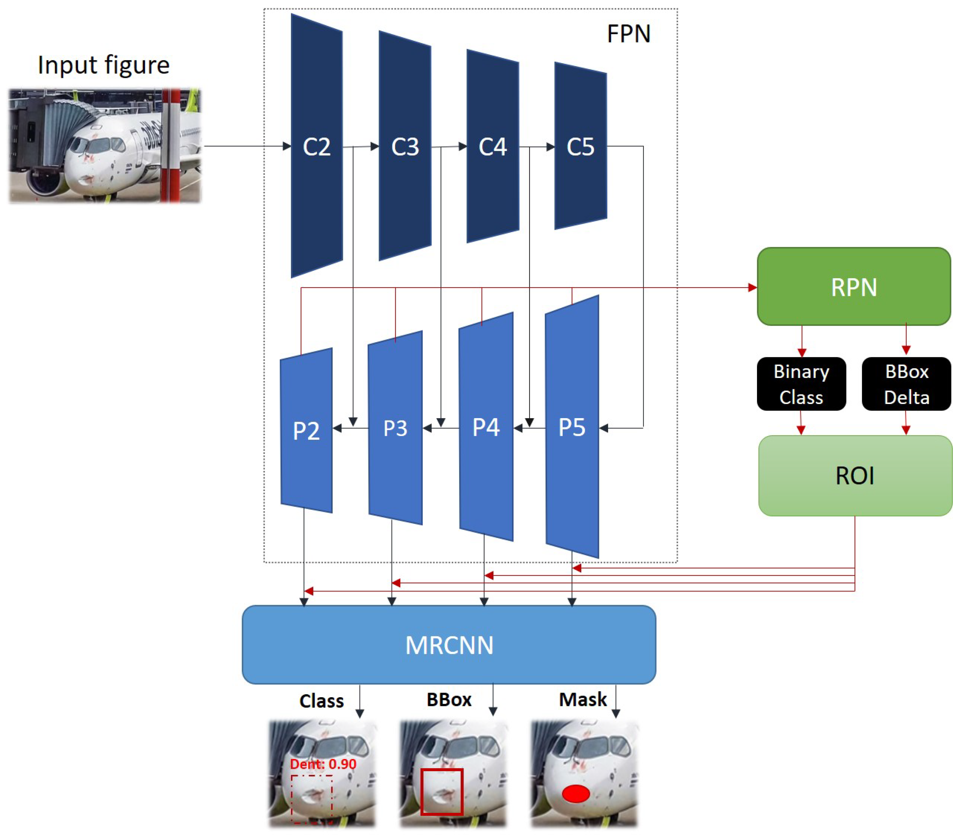
2.1. Dent Detection within MASK R-CNN

As mentioned earlier, detecting dents is not more different than an object detection task and is basically finding an ‘object’ (or region) within an object. Object detection from the simplest perspective has several sub-tasks. The following list moves step-by-step through the process depicted in Figure 1 of the MASK R-CNN approach:

• FPN: The input image is fed into a a so-called FPN [22] that forms the backbone structure of the MASK R-CNN. An FPN or Feature Pyramid Network is a basic component needed in detecting objects at different scales. As shown in Figure 1, the FPN applied in the MASK R-CNN method consists of several convolution blocks (C2 up-to C5) and Pooling blocks (P2 up-to P5). There are in literature several candidates, like ResNet [23] or VGG [24], to represent the FPN. For this study, a ResNet101 network has been used as FPN.
• RPN: The image when passed through the FPN returns the feature maps. These are basically a relatively good initial estimate of regions within the image where one can look for the objects of interest. These feature maps are fed into an RPN, or Region Proposed Network, which are fully convolutional networks that simultaneously predict multiple Anchor boxes and object scores at each position.
• Binary Classification: The former mentioned Anchor boxes are assigned a probability arising from the object scores mentioned earlier, if the object found within the anchor belongs to an object class of interest YES or NO. For example, in our case study, the outcome would be a selection between ‘Dent’ or ‘aircraft skin / background without Dent’.
• BBox Delta: The RPN also returns a bounding box regressor for adjusting the anchors to better fit the object.
• ROI: Combining the information obtained from the Binary Classification and BBox Delta and passing it on to the ROI pooling layer, it is likely that, after the RPN step, there are proposals with no classes assigned to them. One can take each proposal and crop it such that each proposal contains an object. This is exactly what the ROI pooling layer does: It extracts fixed sized feature maps for each anchor.
• MRCNN: The results from the ROI pooling layer is directed toward the MRCNN layer and generates three output streams, i.e.
• Classification: The object is classified as being a ‘Dent’ or ‘No Dent’ with a certain probability assigned.
• Bounding Box: Around the object, a Bounding Box is generated with an optimal fit.
• Mask: Since aircraft dents don’t have a clearly defined shape, arriving at square/rectangular shaped Bounding Box is not sufficient. As a final step, a semantic segmentation is applied, i.e., pixel-wise shading of the class of interest.

In the following part, we discuss the data preparation and the implementation of the concept on real-life aircraft images using MASK R-CNN. The authors have adopted the code taken from [25] such that it can be used to identify dents on aircraft structures. In order to reduce the computational time to train the MASK R-CNN, we have applied transfer learning [26] with a warm restart (shown in Figure 2) and taken the initial weights from [27]. By pre-training the neural network on the COCO data set, we then re-use it on our target data set as the lower layers are already trained on recognizing shapes and sizes from different object classes. In this way, we refine the upper layers for our target data set (aircraft structures with dents).

The most crucial element before training the model is setting up a proper environment, where the core computations are performed. Here, we resort to Google Colab in combination with Python, Jupyter notebook. Google Colab is a free, in-the-browser, collaborative programming environment that provides an interactive and easy to use platform for deep learning researchers and engineers to work on their datascience projects. There is no need for the user to follow complex and tedious procedures to install software, associated packages, worry about data management, and computational resources (CPU/GPU/TPU). All is pre-configured and the user can focus directly on the research questions. Google Colab is a perfect environment for testing Deep Learning based projects before going into production settings and also provides loads of extras, like documenting your work in Markdown, Version control, and Cloning.

2.2. Data Processing for Prediction Improvement

In this paper, we aim to improve the prediction performance of the proposed approach explained above by using some data processing techniques such as augmentations (Section 2.2.1) and by adopting some hierarchical detection system, which adds another classifier before applying the masked RCNN (Section 2.2.2).

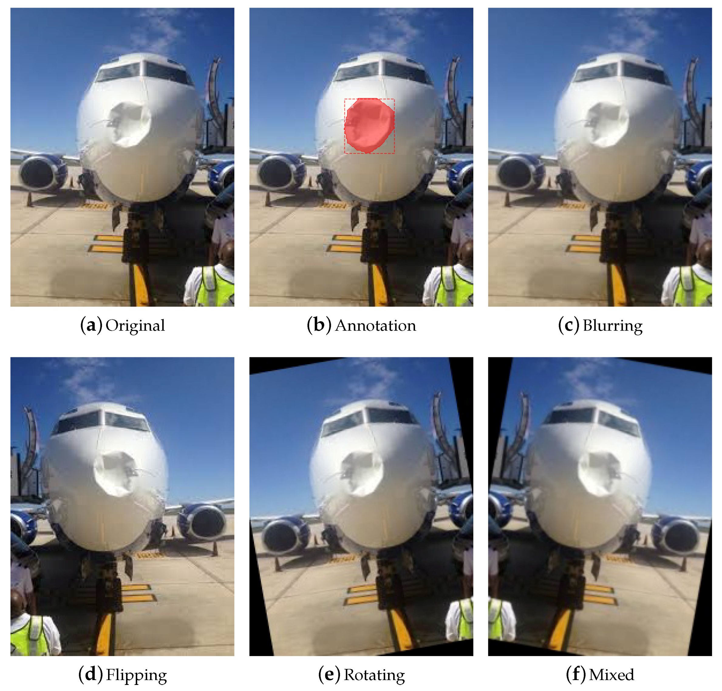
2.2.1. Augmentation Methods

Image augmentation is a technique which aims at generating new images from already existing ones through a wide range of operations including resizing, flipping, cropping, etc. The purpose of this approach is to create diversity, avoid overfitting, and improve generalizability [28]. In order to improve the prediction performance, we suggest applying augmentation methods particularly flipping, rotating, and blurring before training the dataset so that we could increase variety in the training dataset.

By augmentation methods, we produce modifications of the existing images while keeping the dents’ annotations unaffected. Hence, the approach generates new samples with the same label and annotations from already existing ones by visually changing them. In order to prevent damaging the dents’ images and preserve the image quality, it was decided to use soft augmentation techniques. The techniques were randomly applied to the same image together using a Python library known by imgaug [29]. An example is provided in Figure 3 to illustrate the effects of these techniques.

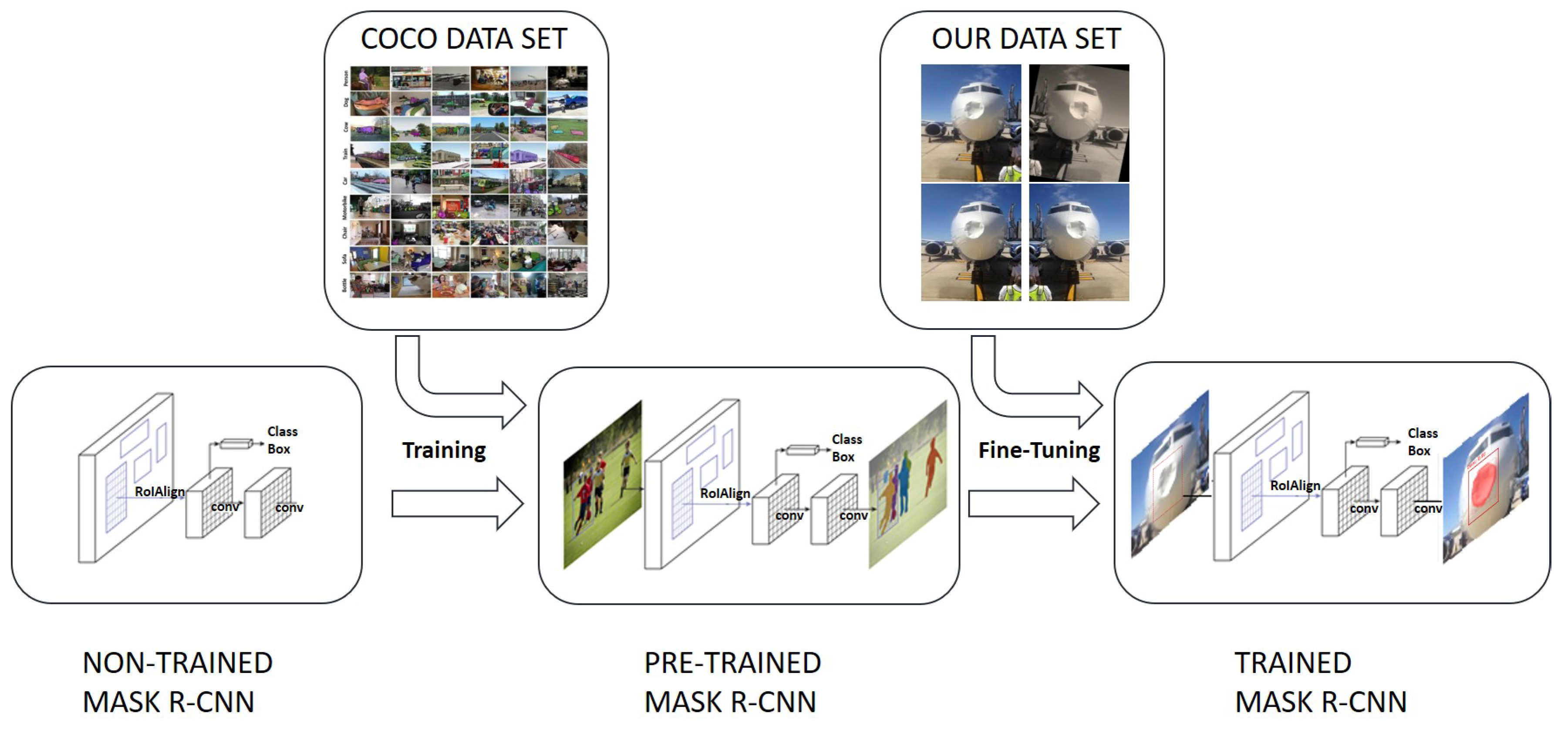
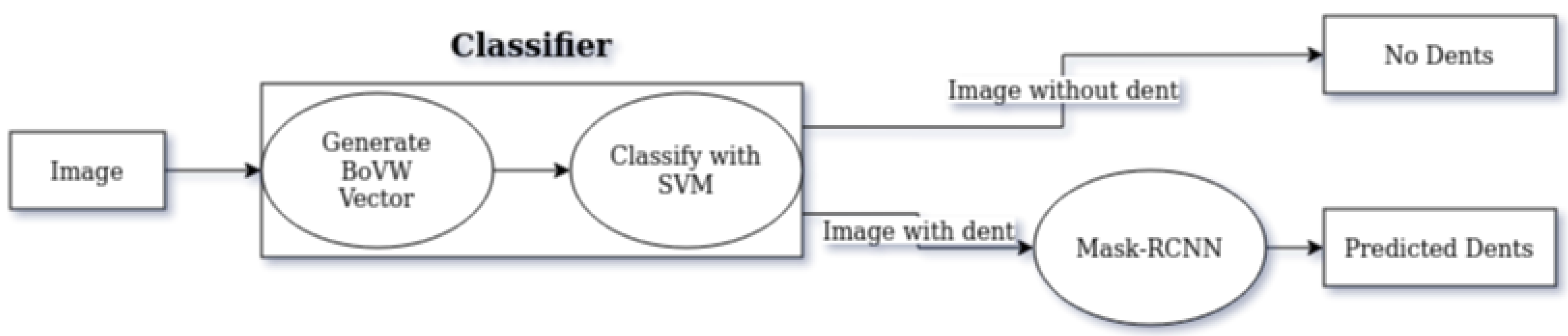
2.2.2. Hierarchical Modeling Approach

When the given dataset includes images that do not have any dents, the Mask R-CNN model may predict some dents on. This would lead to false positives that would decrease precision. To avoid mispredictions on images without dents, we propose to use another classifier, which is trained to detect whether a given image has dents or not. It is called a ‘pre-classifier approach’ in the rest of the paper. As it is demonstrated in Figure 4, this classifier works as a filter. That is, if the pre-classifier labels the given image as having no dents, then the system will output ‘No dents’. Otherwise, the image will be given to the Mark-RCNN model to predict the dents in the given image.

This approach will significantly increase the precision value. However, it may slightly decrease the recall value when an image with dents is predicted as without dents. For classification, we use Bag of Visual Words (BoVW) [30] to generate a vector which can be processed by the classifier namely Support Vector Machine (SVM) [31]. The prediction performance of this classifier is measured and reported in

Table 1. The performance results of the classification model.

	Accuracy	Precision	Recall	F1
Training	97.04%	97.0%	97.0%	97.0%
Test	88.82%	89.9%	88.8%	88.7%

For each fold, a pre-classifier was trained on corresponding train set and the metrics are calculated on corresponding test set. In this table, the metrics are the mean of the metrics of all folds.

. This classifier correctly predicts whether or not there is a dent on the nearly 88% of the images. It is worth noting that the SVM predicts only whether there is a dent or not in the given images while the Mask-RCNN detects the area of the dents.

3. Experimental Results

This section provides an overview of the performance metrics, experimental set-up, and a summary of the key results.

3.1. Model Performance Evaluation

This section presents the evaluation criteria used to assess model performance. As explained above, Mask R-CNN is used to detect the dents on the given aircraft images (i.e., aircraft defects). From the point of view of the decision makers utilizing such a decision-support system, detecting the dent area is more important than calculating the exact area of the dents accurately. Therefore, this work focuses on accurately detecting the dents and measuring the performance by considering how well the dent predictions are made. For this purpose, the well known prediction performance metrics such as precision, recall, and F1 scores are used. In this study, precision measures the percentage of truly detected dents among the dent predictions by the given model (i.e, the percentage of detected dents that were correctly classified), while recall measures what percentage of the dents predictions that are correctly detected.

Formally, Equations (1) and (2) show how to calculate the precision and recall respectively where:

• TP: denotes the true positives and is equal to the number of truly detected dents (i.e., the number of dent predictions, which is correct according to the labeled data).
• FP: denotes the false positives and is equal to the number of falsely detected dents (i.e., the number of dent predictions, which are not correct accordingly to the labeled data).
• FN: denotes the false negatives and is equal to the number of dents, which are not detected by the model (i.e., the number of dents labeled in the original data, but the model could not detect them):

$$Precision=\frac{TP}{TP+FP}$$

(1)

$$Recall=\frac{TP}{TP+FN}$$

(2)

In addition to the above metrics, we also consider an extra performance metric, called $F_{\beta }$-score ($F_{\beta }$ measure). This metric is basically a weighted combination of the Precision and Recall. In addition, the range of the $F_{\beta }$-score is between zero and one where higher values are more desired. In this study, we took two different beta values into consideration which are 1 and 2. $F_1$ conveys the balance between precision and recall while $F_2$ weighs recall higher than precision:

$$F_{\beta }=(1+{\beta }^2)\ast \frac{Precision\ast Recall}{{\beta }^2\ast Precision+Recall}$$

(3)

3.2. Experimental Setup

This section describes the experimental setup and characteristics of datasets used to train and test the convolutional neural network.

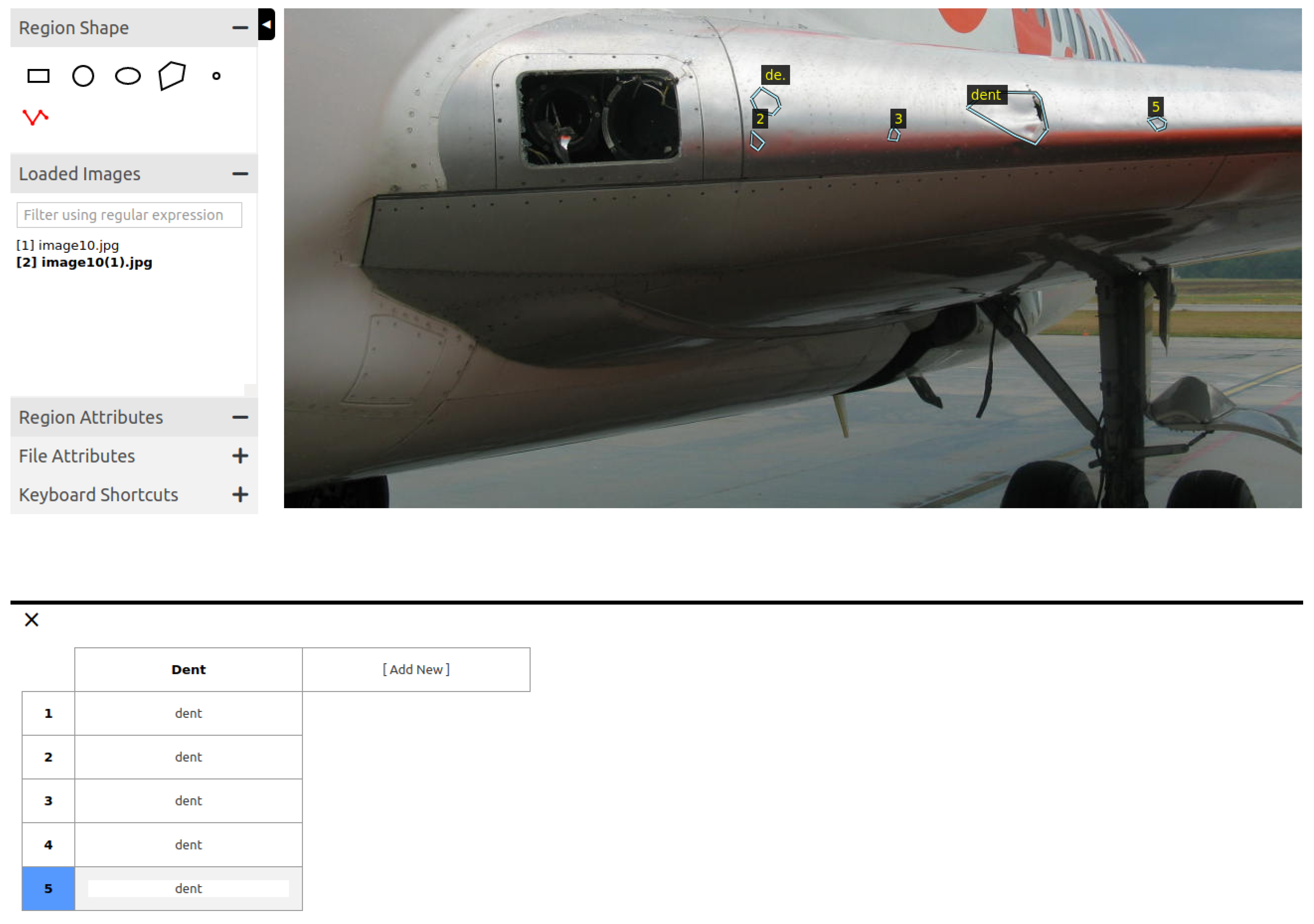
3.2.1. Data Collection and Annotation

The first step in this research involves collecting images of aircraft dents from different sources. To the best of the authors’ knowledge, this is the first study which focuses on automating aircraft dents’ detection. Therefore, there was no image database for aircraft dents publicly available. Thus, a key first step was to develop an aircraft dents database from scratch. This was achieved by taking photos of aircraft dents at Abu Dhabi Polytechnic Hangar (Figure 5) and combining it with online images that had one or multiple aircraft dents.

The 56 aircraft dents’ images used for training the model were diverse in terms of size, location, and number of dents as described below:

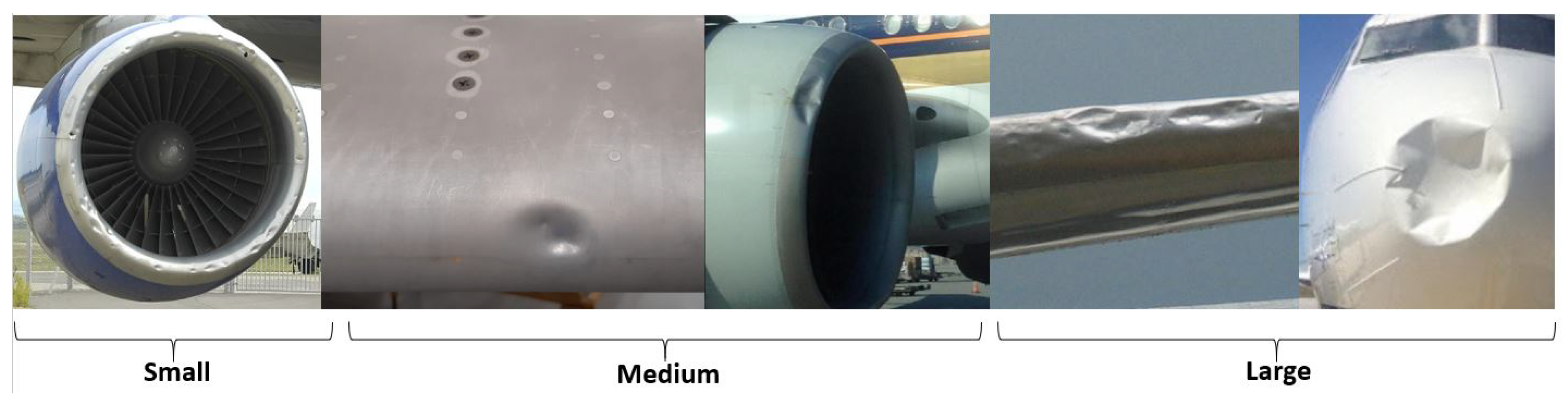
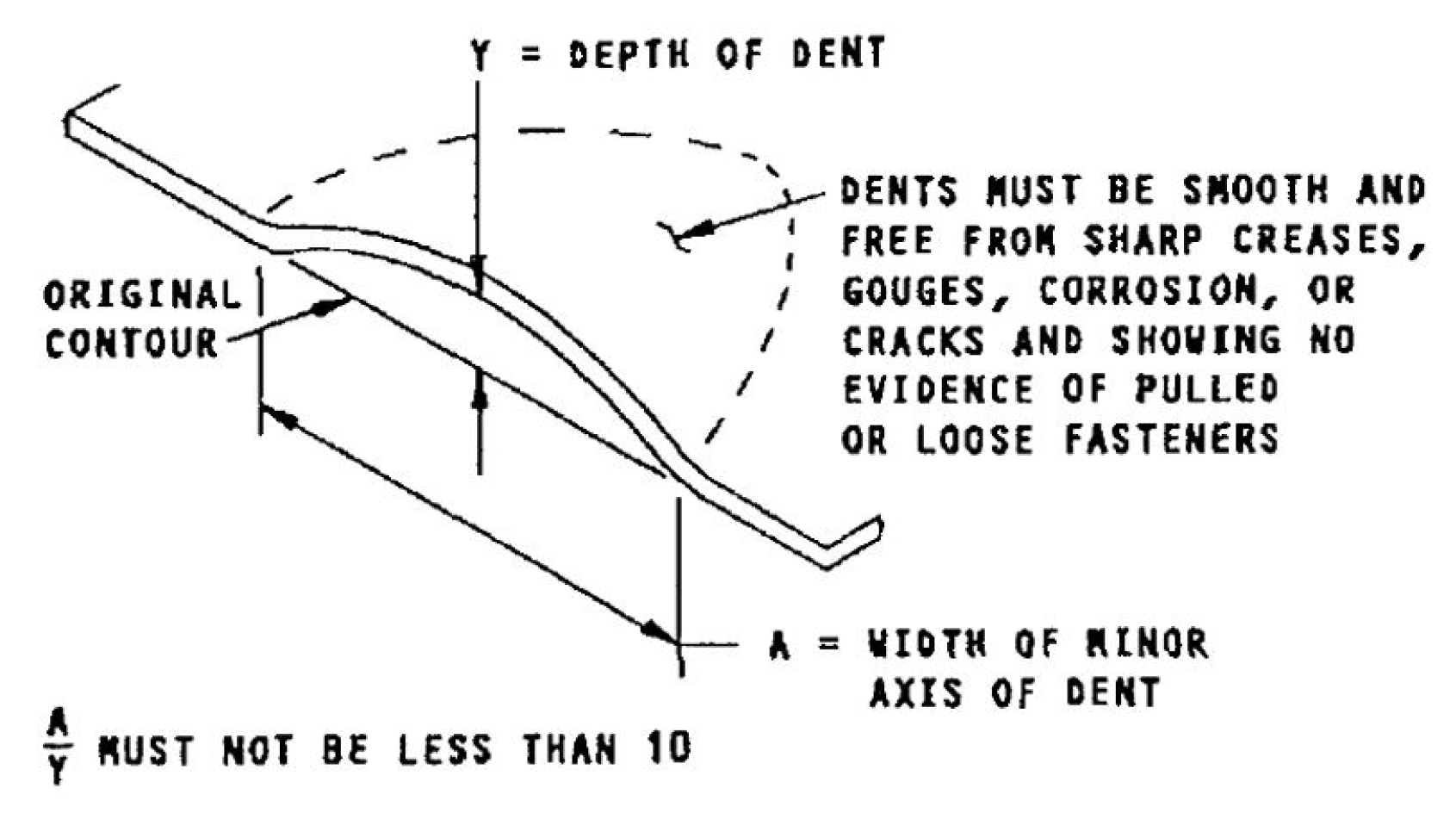
• Size of Dents: The deep learning model was trained with images of aircraft dents of varying sizes ranging from small to large. Figure 6 shows the smallest dents used in this study on the left-hand side, and the largest dents on the right-hand side. These were typically found on the aircraft radome. It should be noted that the aim of this paper was to detect both allowable and non-allowable dents (Figure 7). Additional functionalities can be added to the AI system to detect only critical dents when used in combination with 3D scanning technology.
• Location of Dents: The dents are located on five main areas in the aircraft, namely the Wing Leading Edge, radome, engine cowling, doors, and leading edge of the horizontal stabilizer. These are typical areas on the aircraft where dents can be found as a result of bird strike, hail damage, or ground accidents.
• Number of Dents: As can be seen in Figure 6, while some images only had one dent on them, other images had dozens of dent.

Since the total number of images was small (56 images), we have involved highly experienced aircraft maintenance engineers during the annotation process in order to accurately label the location of the dents in each image as shown in Figure 8.

3.2.2. Datasets’ Characteristics

Based on the original dataset in [1], we have prepared six different datasets that are described below and summarized in

Table 2. Data set description.

	Image with Dents	Images without Dents	Scope
Dataset 1	56	49	Aircraft
Dataset 2	26	20	Wing
Dataset 3	56	0	Aircraft
Dataset 4	56	0	Aircraft
Dataset 5	56	49	Aircraft
Dataset 6	56	49	Aircraft

.

• Dataset 1: This dataset is a combination of the original dataset which contains 56 images of aircraft dents [1] and a new dataset of 49 images without dents. The annotation in the original dataset used in [1] has also been improved through involving more experts to reach consensus and later verified by another expert. Briefly, Dataset 1 has nearly balanced images with dents and without dents (105 images in total).
• Dataset 2: This dataset is a subset of dataset 1 and contains 46 wing images in total—26 that have dents, and 20 without dents.
• Dataset 3: This dataset contains half the number of images in the original dataset which contain images with dents only [1], combined with augmented images of the remaining half. Note that we applied the mixed augmentation technique as shown in Figure 3.
• Dataset 4: This dataset contains all the images with dents in the original dataset (56 images with dents) in combination with their augmented version.
• Dataset 5: This dataset contains half the number of images in dataset 1 combined with the augmented images of the remaining half. This dataset contains both images with dents and without dents.
• Dataset 6: This dataset contains all the images with dents in dataset 1 (56 images with dents and 49 images without dents) in combination with their augmented version.

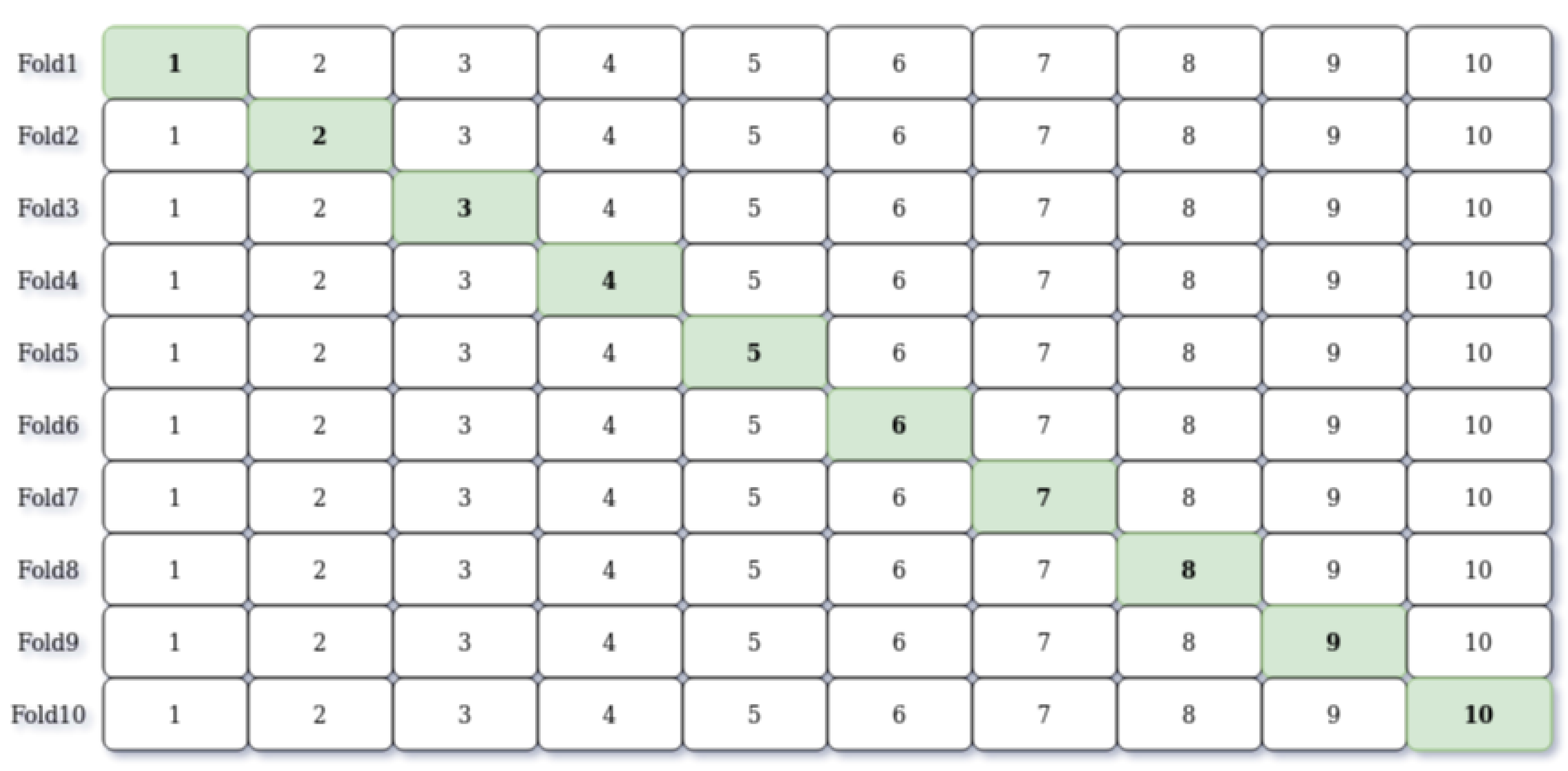
3.2.3. Training and Test Split

The main challenge in this study faced was data scarcity. In addition to using clean and clearly labeled data, we used a 10-fold cross-validation [32] in order to have a diverse pool of training and test data for a robust evaluation. In this approach, the original dataset was split into 10 equally sized parts. By combining these parts in a systematic way (i.e., one for test, the rest for training), we create 10 different combinations of training and test dataset as shown in Figure 9.

After training the network model on the training set of each fold and testing on the associated test sets separately, an expert checked and compared the predictions with the labeled data for each fold and calculate the true positives TP, false negatives FN, and false positives FP. It is worth noting that we have used a Mask R-CNN that has already been trained to detect car dents [33]. Therefore, even with a small dataset, we could be able to detect the areas of dents on the aircraft dataset. This concept is also known as transfer learning.

3.2.4. Training Approach

Thanks to transfer learning, the ResNet part of the model can extract some visual features that can be utilized in this study without any additional training. However, the other parts of the model must be trained to utilize these visual features. Therefore, the heads of the model (excluding ResNet) must be trained. Firstly, the ResNet weights are frozen, then the model is trained 15 epochs for a dataset of approximately 50 images. Note that the number of epochs are tuned according to the size of the dataset (e.g., 30 for a dataset of 100 images). In addition to this, the ResNet part of the model should also be trained to get better results because the ResNet may extract more useful visual features after training. Therefore, the weights of the model, including ResNet, continued training five more epochs (also tuned according to the size of the dataset). Briefly, the model is trained for 15 epochs without ResNet, then 5 more epochs with ResNet, and a total of 20 epochs is trained.

4. Experimental Results and Analysis

This section provides the experimental results showing the prediction performance of the proposed approach in detail. In particular, we study the effect of certain dataset modifications such as adding images without dents (Section 4.1), filtering the dataset by focusing only a part of the airplane (Section 4.2), image augmentation (Section 4.3) as well as the changes in the training such as increasing the number of epochs (Section 4.4) and incorporating a pre-classifier to the prediction process (Section 4.5). In the following section, we present the average evaluation values of 10-cross validation results where experiment evaluations per each fold are also given in Appendix A.

4.1. The Effect of Dataset Balance

The main challenge faced was the small size of the dents dataset. To overcome this obstacle, we ensured that the dataset is clean and accurately labeled by involving experienced aircraft engineers. In real life, there are images with and without dents. Therefore, it is important to involve negative examples (in our case images without dents) to obtain a more balanced dataset. To achieve this, the initial dataset was extended by adding additional images without dents to improve prediction performance (see Dataset 1). The model is trained 20 epochs in total on Dataset 1 as it is in the original dataset [1].

Table 3. The results of the effect of Dataset balance.

Dataset	Epoch	Train Size	Test Size	Precision	Recall	${\mathit{F}}_1$ Score	${\mathit{F}}_2$ Score
Original Dataset [1]	15 + 5	49.5	5.5	69.13%	57.32%	62.67%	59.35%
Dataset 1	15 + 5	94.5	10.5	21.56%	66.29%	32.54%	46.85%

shows the performance comparison on Dataset 1 with the original dataset.

With the extended dataset, a higher recall value (66.29% versus 57.32%) and lower precision value (21.56% versus 69.13%) have been achieved compared to the baseline experiment conducted in [1]. In this context, recall is more important than precision. Detecting an approximate location of dents correctly is of paramount importance. Our primary aim is not to miss any dents to help human experts analyzing thousands of images. In such a case, it may be admissible if the algorithm may sometimes detect a dent location, which does not exist. In this case, the human expert can give feedback to the system. The detailed results are shown in

Table A1. The Results of Experiment 1: Adding images without dents (Dataset 1).

	Fold 1	Fold 2	Fold 3	Fold 4	Fold 5	Fold 6	Fold 7	Fold 8	Fold 9	Fold 10	Average
Train Size	94	94	94	94	94	95	95	95	95	95	94.5
Test Size	11	11	11	11	11	10	10	10	10	10	10.5
TP	6	5	4	68	5	42	6	8	3	4	15.1
FP	68	72	21	26	37	34	37	46	32	45	41.8
FN	2	5	4	81	1	37	1	2	2	1	13.6
Recall	75.0%	50.0%	50.0%	45.6%	83.3%	53.7%	85.7%	80.0%	60.0%	80.0%	66.29%
Precision	8.1%	6.5%	16.0%	72.3%	11.9%	55.3%	14.0%	14.8%	8.6%	8.2%	21.56%

(Recall: 66.29%; Precision: 21.56%; $F_1$-Score: 32.54%; $F_2$-Score: 46.85%).

4.2. The Effect of Specialization in the Dataset

A model with a specific dataset may lead to better results than a model with a generic dataset. Therefore, a subdataset can be prepared by focusing on specific aircraft parts like wing or engine to train a branched model instead of a generic model. Since aircraft dents are often prevalent in areas like the wing leading edge, engines, and radome, this study has focused on the wing because of the data availability. Therefore, we filter the Dataset 1 by focusing on only aircraft wings. The wing Dataset 2 was therefore used to train a branched model that is able to detect wing dents. According to the results shown in

Table 4. The results of the effect of specialization in dataset.

Dataset	Epoch	Train Size	Test Size	Precision	Recall	${\mathit{F}}_1$ Score	${\mathit{F}}_2$ Score
Dataset 1	15 + 5	94.5	10.5	21.56%	66.29%	32.54%	46.85%
Dataset 2	15 + 5	41.4	4.6	69.88 %	54.39%	61.17%	56.91%

, the precision value is much higher than in the Dataset 1 (69.88% versus 21.56%), but the recall value is lower (54.39% versus 66.29%). Furthermore, $F_1$ score (61.17% versus 32.54%) and $F_2$ score (56.91% versus 46.85%) are higher than the Dataset 1 due to higher precision value. The corresponding results are shown in

Table A2. The Results of Experiment 2: Filtering the dataset by focusing on only aircraft wings (Dataset 2).

	Fold 1	Fold 2	Fold 3	Fold 4	Fold 5	Fold 6	Fold 7	Fold 8	Fold 9	Fold 10	Average
Train Size	41	41	41	41	41	41	42	42	42	42	41.4
Test Size	5	5	5	5	5	5	4	4	4	4	4.6
TP	2	3	5	6	15	1	1	1	9	1	4.4
FP	2	0	2	1	5	1	5	0	0	1	1.7
FN	1	2	1	2	12	2	3	1	11	1	3.6
Recall	66.7%	60.0%	83.3%	75.0%	55.6%	33.3%	25.0%	50.0%	45.0%	50.0%	54.39%
Precision	50.0%	100.0%	71.4%	85.7%	75.0%	50.0%	16.7%	100.0%	100.0%	50.0%	69.88%

(Recall: 54.39%; Precision: 69.88%; $F_1$-Score: 61.17%; $F_2$-Score: 56.91%).

4.3. The Effect of Augmentation Process

Image augmentation is a technique, which aims at generating new images from already existing ones through a wide range of operations including resizing, flipping, cropping, and so on. The purpose of this approach is to create diversity, avoid overfitting, and improve generalizability [28]. To investigate whether the augmentation technique could improve the prediction performance, we applied augmentation augmentation techniques namely flipping, rotating, and blurring (Section 2.2.1) on the original dataset in different ways as explained below and compared their performance with the case of no augmentation as shown in

Table 5. The results of the effect of augmentation process.

Dataset	Augmentation	Epoch	Train Size	Test Size	Precision	Recall	${\mathit{F}}_1$ Score	${\mathit{F}}_2$ Score
Original Dataset [1]	No	15 + 5	49.5	5.5	69.13%	57.32%	62.67%	59.35%
Dataset 3	Yes	15 + 5	50.4	5.6	60.32%	68.08%	63.96%	66.37%
Dataset 4	Yes	15 + 5	100.8	5.6	60.60%	59.52%	60.06%	59.73%
Dataset 5	Yes	15 + 5	94.5	10.5	27.02%	69.30%	38.88%	52.78%
Dataset 6	Yes	15 + 5	189	10.5	36.80%	62.83%	46.41%	55.04%

.

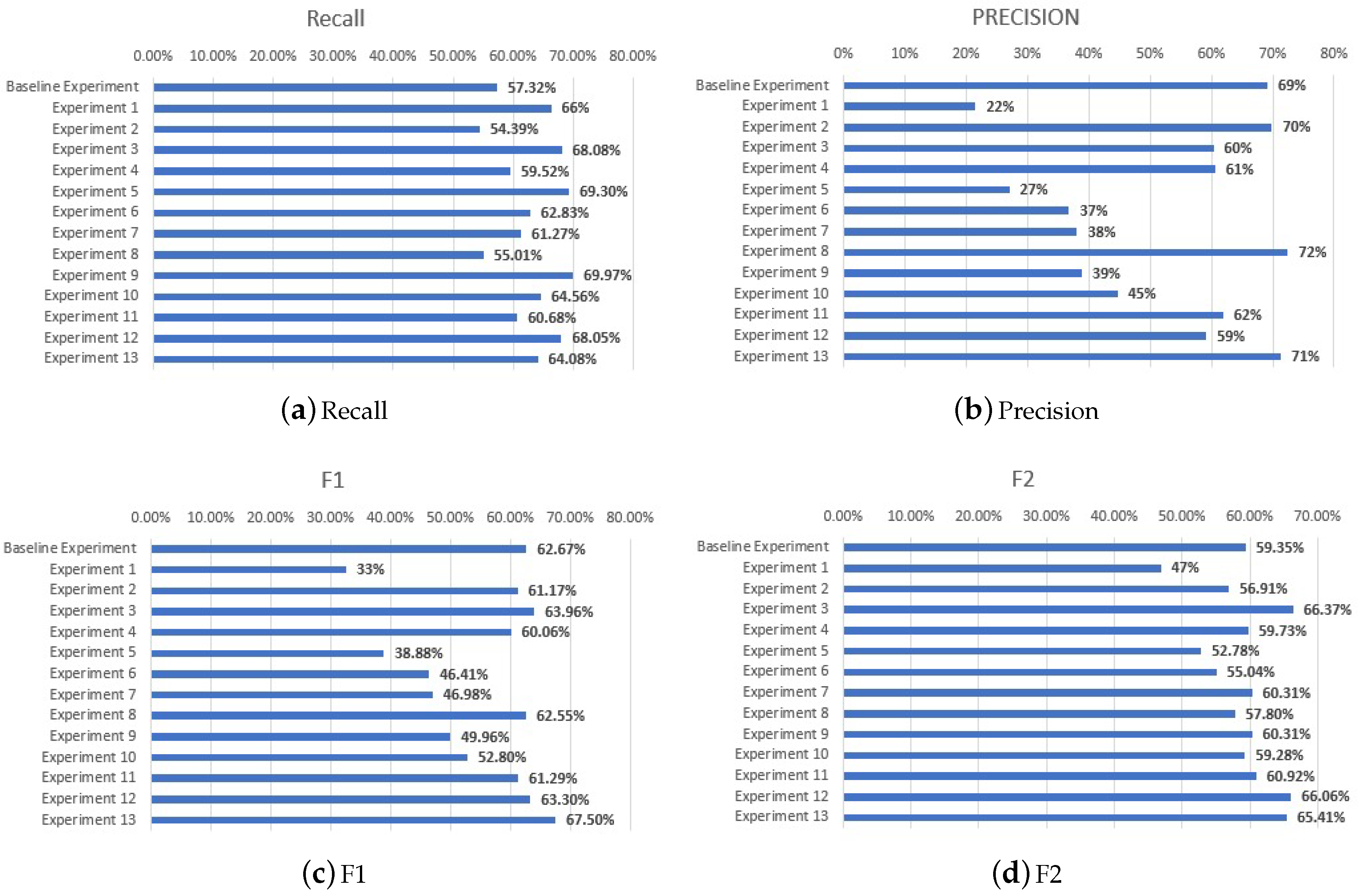
• Flipping, rotating, and blurring 50% of the dataset: Half of the images were transformed using three augmentation techniques namely flipping, rotating, and blurring (Section 2.2.1), while the other half remained the same resulting into a new dataset [Dataset 3]. The recall value and $F_1$ score is higher than the baseline experiment (68.08% versus 57.32% and 63.96% versus 62.67%). In addition, the highest $F_2$ score among all experiments are obtained in this experiment, although the precision is lower than the baseline experiment (60.32% versus 69.13%). The detailed results are shown in

  Table A3. The Results of Experiment 3: Augment 50% of dataset (Dataset 3).

  	Fold 1	Fold 2	Fold 3	Fold 4	Fold 5	Fold 6	Fold 7	Fold 8	Fold 9	Fold 10	Average
  Train Size	50	50	50	50	50	50	51	51	51	51	50.4
  Test Size	6	6	6	6	6	6	5	5	5	5	5.6
  TP	34	8	5	22	5	9	5	4	25	27	14.4
  FP	2	12	5	13	5	4	2	16	18	4	8.1
  FN	26	2	4	3	1	4	0	1	52	49	14.2
  Recall	56.7%	80.0%	55.6%	88.0%	83.3%	69.2%	100.0%	80.0%	32.5%	35.5%	68.08%
  Precision	94.4%	40.0%	50.0%	62.9%	50.0%	69.2%	71.4%	20.0%	58.1%	87.1%	60.32%

  (Recall: 68.08%; Precision: 60.32%; $F_1$-Score: 63.97%; $F_2$-Score: 66.37%).
• Flipping, rotating, and blurring the complete dataset: Instead of partially augmenting the dataset, we augment all images and use both original and augmented images for training. Consequently, the dataset [Dataset 4] becomes twice the size of original dataset [Dataset 4] in the training phrase. Note that the same image augmentation techniques have been used (flipping, rotating and blurring). The detailed results are shown in

  Table A4. The Results of Experiment 4: Augment the complete dataset (Dataset 4).

  	Fold 1	Fold 2	Fold 3	Fold 4	Fold 5	Fold 6	Fold 7	Fold 8	Fold 9	Fold 10	Average
  Train Size	100	100	100	100	100	100	102	102	102	102	100.08
  Test Size	6	6	6	6	6	6	5	5	5	5	5.6
  TP	12	7	6	20	6	6	5	4	22	7	9.5
  FP	3	13	8	9	3	4	1	11	12	2	6.6
  FN	48	3	3	5	0	8	0	1	61	69	19.8
  Recall	20.0%	70.0%	66.7%	80.0%	100.0%	42.9%	100.0%	80.0%	26.5%	9.2%	59.52%
  Precision	80.0%	35.0%	42.9%	69.0%	66.7%	60.0%	83.3%	26.7%	64.7%	77.8%	60.60%

  (Recall: 59.52%; Precision: 60.60%; $F_1$-Score: 60.06%; $F_2$-Score: 59.73%).
• Flipping, rotating, and blurring 50% of the dataset containing images with and without dent: This experiment is a combination of the first augmentation approach and adding the images without a dent approach. In other words, the first image augmentation approach is applied on Dataset 1 which contains both 56 images with dents and 49 images without dents. The recall value is slightly higher than the first augmentation on the original dataset (69.30% versus 68.08%) while the precision value is much lower than the baseline experiment (27.02% versus 69.13%). The corresponding results are shown in

  Table A5. The Results of Experiment 5: Augment 50% of dataset containing images with and without dents (Dataset 5).

  	Fold 1	Fold 2	Fold 3	Fold 4	Fold 5	Fold 6	Fold 7	Fold 8	Fold 9	Fold 10	Average
  Train Size	50	50	50	50	50	50	51	51	51	51	50.4
  Test Size	6	6	6	6	6	6	5	5	5	5	5.6
  TP	5	7	7	50	6	27	6	8	3	4	12.3
  FP	41	44	19	29	17	33	14	28	15	22	26.2
  FN	3	3	1	99	0	53	1	2	2	1	16.5
  Recall	62.50%	70.00%	87.50%	33.56%	100.00%	33.75%	85.71%	80.00%	60.00%	80.00%	69.30%
  Precision	10.87%	13.73%	26.92%	63.29%	26.09%	45.00%	30.00%	22.22%	16.67%	15.38%	27.02%

  (Recall: 69.30%; Precision: 27.02%; $F_1$-Score: 38.88%; $F_2$-Score: 52.78%).
• Flipping, rotating, and blurring the complete dataset containing images with and without dents: This experiment is a combination of the second augmentation approach and adding additional images without a dent approach. In other words, the second image augmentation approach is applied on Dataset 1, which contains both 56 images with dent and 49 images without dent. In this case, the recall value is higher than the second augmentation on the original dataset (62.83% versus 59.52%), but the precision value is lower (36.80% versus 60.60%). Additionally, the recall is also higher than the baseline experiment [1] (62.83% versus 57.32%). The corresponding results are shown in

  Table A6. The Results of Experiment 6: Augment the complete dataset containing images with and without dents (Dataset 6).

  	Fold 1	Fold 2	Fold 3	Fold 4	Fold 5	Fold 6	Fold 7	Fold 8	Fold 9	Fold 10	Average
  Train Size	94	94	94	94	94	95	95	95	95	95	94.5
  Test Size	11	11	11	11	11	10	10	10	10	10	10.5
  TP	4	6	3	67	6	12	7	8	3	4	12
  FP	14	23	6	9	27	10	17	17	6	7	13.6
  FN	4	4	5	80	0	67	0	2	2	1	16.5
  Recall	50.00%	60.00%	37.50%	45.58%	100.00%	15.19%	100.00%	80.00%	60.00%	80.00%	62.83%
  Precision	22.22%	20.69%	33.33%	88.16%	18.18%	54.55%	29.17%	32.00%	33.33%	36.36%	36.80%

  (Recall: 62.83%; Precision: 36.80%; $F_1$-Score: 46.41%; $F_2$-Score: 55.04%).

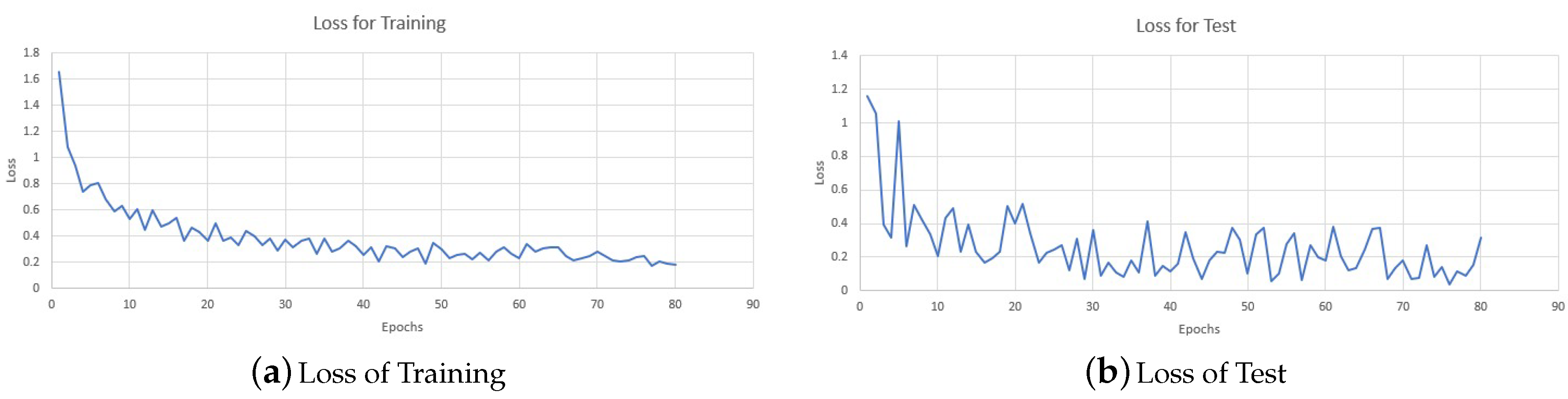
4.4. The Effect of Number of Epochs in Training

When we train a model in ML, there are a number of hyper parameters, which may influence the performance of the model. One of them is the stopping criterion (i.e., convergence condition and number of epochs). In this work, the training process is stopped when it reaches a predetermined number of epochs (e.g., 15 + 5). We use the same number of epochs for aforementioned experiments. In this section, we show the effect of the number of epochs which corresponds to how many times we traverse over all training instances and update the parameters accordingly on the prediction performance.

As it can be seen in

Table 6. The results of the effect of training parameters.

Dataset	Augmentation	Epoch	Train Size	Test Size	Precision	Recall	${\mathit{F}}_1$ Score	${\mathit{F}}_2$ Score
Dataset 1	No	15 + 5	94.5	10.5	21.56%	66.29%	32.54%	46.85%
Dataset 1	No	30 + 10	94.5	10.5	38.10%	61.27%	46.98%	54.62%
Dataset 4	Yes	15 + 5	100.8	5.6	60.60%	59.52%	60.06%	59.73%
Dataset 4	Yes	30 + 10	100.8	5.6	72.48%	55.01%	62.55%	57.80%
Dataset 5	Yes	15 + 5	94.5	10.5	27.02%	69.30%	38.88%	52.78%
Dataset 5	Yes	30 + 10	94.5	10.5	38.85%	69.97%	49.96%	60.31%
Dataset 6	Yes	15 + 5	189	10.5	36.80%	62.83%	46.41%	55.04%
Dataset 6	Yes	60 + 20	189	10.5	44.66%	64.56%	52.80%	59.28%

, increasing the value of epoch parameter (i.e., iterating the training instance more while training) drastically increased the precision value for all experiments. Although this approach slightly decreased the recall value, the $F_1$ and $F_2$ scores were still better for the larger epoch values. It is worth noting that the Dataset 4 with a doubled epoch number has the highest precision value among all experiments (72.48%) while the Dataset 5 has the highest recall value (69.97%). The detailed results of Dataset 1, Dataset 4, Dataset 5, and Dataset 6 with a doubled epoch number are shown in

Table A7. The Results of Experiment 7: Adding images without dents (Dataset 1), with a larger number of epochs.

	Fold 1	Fold 2	Fold 3	Fold 4	Fold 5	Fold 6	Fold 7	Fold 8	Fold 9	Fold 10	Average
Train Size	94	94	94	94	94	95	95	95	95	95	94.5
Test Size	11	11	11	11	11	10	10	10	10	10	10.5
TP	3	5	5	59	6	23	5	8	3	4	12.1
FP	14	21	12	6	8	19	13	5	22	12	13.2
FN	5	5	3	81	0	56	2	2	2	1	15.7
Recall	37.50%	50.00%	62.50%	42.14%	100.00%	29.11%	71.43%	80.00%	60.00%	80.00%	61.27%
Precision	17.65%	19.23%	29.41%	90.77%	42.86%	54.76%	27.78%	61.54%	12.00%	25.00%	38.10%

,

Table A8. The Results of Experiment 8: Augment the complete dataset (Dataset 4), with a larger number of epochs.

	Fold 1	Fold 2	Fold 3	Fold 4	Fold 5	Fold 6	Fold 7	Fold 8	Fold 9	Fold 10	Average
Train Size	100	100	100	100	100	100	102	102	102	102	100.08
Test Size	6	6	6	6	6	6	5	5	5	5	5.6
TP	13	6	6	17	5	9	4	2	20	30	11.2
FP	1	3	6	4	2	4	1	3	6	1	3.1
FN	45	4	3	8	1	5	1	3	57	46	17.3
Recall	22.41%	60.00%	66.67%	68.00%	83.33%	64.29%	80.00%	40.00%	25.97%	39.47%	55.01%
Precision	92.86%	66.67%	50.00%	80.95%	71.43%	69.23%	80.00%	40.00%	76.92%	96.77%	72.48%

,

Table A9. The Results of Experiment 9: Augment 50% of dataset containing images with and without dent (Dataset 5), with a larger number of epochs.

	Fold 1	Fold 2	Fold 3	Fold 4	Fold 5	Fold 6	Fold 7	Fold 8	Fold 9	Fold 10	Average
Train Size	94	94	94	94	94	95	95	95	95	95	94.5
Test Size	11	11	11	11	11	10	10	10	10	10	10.5
TP	4	8	6	72	6	23	7	8	3	4	14.1
FP	17	18	11	13	13	13	17	8	9	17	13.6
FN	4	2	2	86	0	56	0	2	2	1	15.5
Recall	50.00%	80.00%	75.00%	45.57%	100.00%	29.11%	100.00%	80.00%	60.00%	80.00%	69.97%
Precision	19.05%	30.77%	35.29%	84.71%	31.58%	63.89%	29.17%	50.00%	25.00%	19.05%	38.85%

and

Table A10. The Results of Experiment 10: Augment the complete dataset containing images with and without dents (Dataset 6), with a larger number of epochs.

	Fold 1	Fold 2	Fold 3	Fold 4	Fold 5	Fold 6	Fold 7	Fold 8	Fold 9	Fold 10	Average
Train Size	188	188	188	188	188	190	190	190	190	190	189
Test Size	11	11	11	11	11	10	10	10	10	10	10.5
TP	4	7	6	47	5	26	6	8	3	3	11.5
FP	11	14	10	7	17	8	14	12	3	4	10
FN	4	3	2	100	0	53	1	2	2	2	16.9
Recall	50.00%	70.00%	75.00%	31.97%	100.00%	32.91%	85.71%	80.00%	60.00%	60.00%	64.56%
Precision	26.67%	33.33%	37.50%	87.04%	22.73%	76.47%	30.00%	40.00%	50.00%	42.86%	44.66%

, respectively. A larger number of epochs can also decrease the loss of both training and test sets, as it can be seen in Figure 10, but at some point they do not change the results significantly. According to the given error graph, it can be seen that the low number of epochs would be sufficient to train the model reasonably well enough.

4.5. The Effect of the Pre-Classifier Approach

Lastly, we study the effect of introducing a pre-classifier approach (see Section 2.2.2).

Table 7. The results of the effect of the pre-classifier approach.

Dataset	Augmentation	Classifier	Epoch	Train Size	Test Size	Precision	Recall	${\mathit{F}}_1$ Score	${\mathit{F}}_2$ Score
Dataset 1	No	No	30 + 10	94.5	10.5	38.10%	61.27%	46.98%	54.62%
Dataset 1	No	Yes	30 + 10	94.5	10.5	61.91%	60.68%	61.29%	60.92%
Dataset 5	Yes	No	30 + 10	94.5	10.5	38.85%	69.97%	49.96%	60.31%
Dataset 5	Yes	Yes	30 + 10	94.5	10.5	59.17%	68.05	63.30%	66.06%
Dataset 6	Yes	No	60 + 20	189	10.5	44.66%	64.56%	52.80%	59.28%
Dataset 6	Yes	Yes	60 + 20	189	10.5	71.31%	64.08%	67.50%	65.41%

shows the results of the previous experiments with their corresponding experiments with the pre-classifier. According to these results, it can be seen that precision drastically increases and recall slightly decreases when we adopt the pre-classifer approach. Note that the highest $F_1$ score is gained when we use augmented Dataset 6 with an epoch 60 + 20 with pre-classifier (67.50%). For each dataset, we explain the effect of a pre-classifer in a detailed way below.

Balanced Dataset with a pre-classifier: Regarding the experimental results on Dataset 1, a considerably lower precision value than the baseline experiment’s precision was observed due to a high False Positive. Most of the False Positive predictions (predicting an area as dent where there is no dent) are made on some of the images without dents in Dataset 1. Therefore, a classifier which predicts whether a given image has dents or does not have dents was implemented and used on a test set to avoid mispredictions on the images without dents. Firstly, the pre-classifier predicts an image if it has dent, or not. Then, the Mask-RCNN model extracts the dented areas if the image is classified as an image with dents. Otherwise, it outputs no dents without applying the Mask-RCNN model. We used the Mask-RCNN model trained in Dataset 1. The precision value dramatically increased from 38.10% to 61.91% by reducing some of False Positive detections. In addition, this approach increased not only $F_1$ score (46.98% to 61.29%) but also $F_2$ score (54.62% to 60.92%). However, the pre-classifier predicts some of the images with dents as images without dents, so the recall value slightly decreased (61.27% to 60.68%). The detailed results are shown in

Table A11. The Results of Experiment 11: Adding images without dents (Dataset 1), by testing with a pre-classifier.

	Fold 1	Fold 2	Fold 3	Fold 4	Fold 5	Fold 6	Fold 7	Fold 8	Fold 9	Fold 10	Average
Train Size	94	94	94	94	94	95	95	95	95	95	94.5
Test Size	11	11	11	11	11	10	10	10	10	10	10.5
TP	3	5	5	54	6	23	5	8	3	4	11.6
FP	8	2	6	4	3	3	5	4	7	1	4.3
FN	5	5	3	95	0	56	2	2	2	1	17.1
Recall	37.50%	50.00%	62.50%	36.24%	100.00%	29.11%	71.43%	80.00%	60.00%	80.00%	60.68%
Precision	27.27%	71.43%	45.45%	93.10%	66.67%	88.46%	50.00%	66.67%	30.00%	80.00%	61.91%

(Recall: 60.68%; Precision: 61.91%; $F_1$-Score: 61.29%; $F_2$-Score: 60.92%).

Flipping, rotating, and blurring 50% of the dataset containing images with and without dents by testing with the pre-classifier: We used the pre-classifier with the Mask-RCNN model trained in Dataset 5. This approach significantly increases the precision value, $F_1$ and $F_2$ scores (38.85% to 59.17%, 49.96% to 63.30% and 60.31% to 66.06%). However, the recall value decreases (69.97% to 68.05%) due to the fact that the pre-classifier predicts some of the images with dents as images without dents. The corresponding results are shown in

Table A12. The Results of Experiment 12: Augment 50% of dataset containing images with and without dents (Dataset 5), by testing with the pre-classifier.

	Fold 1	Fold 2	Fold 3	Fold 4	Fold 5	Fold 6	Fold 7	Fold 8	Fold 9	Fold 10	Average
Train Size	94	94	94	94	94	95	95	95	95	95	94.5
Test Size	11	11	11	11	11	10	10	10	10	10	10.5
TP	4	8	6	39	6	23	7	8	3	4	10.8
FP	11	7	7	6	6	3	9	2	3	2	5.6
FN	4	2	2	109	0	56	0	2	2	1	17.8
Recall	50.00%	80.00%	75.00%	26.35%	100.00%	29.11%	100.00%	80.00%	60.00%	80.00%	68.05%
Precision	26.67%	53.33%	46.15%	86.67%	50.00%	88.46%	43.75%	80.00%	50.00%	66.67%	59.17%

(Recall: 68.05%; Precision: 59.17%; $F_1$-Score: 63.30%; $F_2$-Score: 66.06%).

Flipping, rotating, and blurring the complete dataset containing images with and without dents by testing with the pre-classifier: The pre-classifier approach and the Mask-RCNN model trained in Dataset 6 are utilized to decrease False Positive detection on the images without dents. The precision considerably increased (44.66% to 71.31%) and the highest $F_1$ score among all experiments is achieved. In addition, the $F_2$ score increased (59.28% to 65.41%) although the recall value slightly decreased (64.56% to 64.08%) due to misprediction made by the pre-classifier. The detailed results are shown in

Table A13. The Results of Experiment 13: Augment the complete dataset containing images with and without dents (Dataset 6), by testing with the pre-classifier.

	Fold 1	Fold 2	Fold 3	Fold 4	Fold 5	Fold 6	Fold 7	Fold 8	Fold 9	Fold 10	Average
Train Size	188	188	188	188	188	190	190	190	190	190	189
Test Size	11	11	11	11	11	10	10	10	10	10	10.5
TP	4	7	6	40	5	26	6	8	3	3	10.8
FP	7	5	3	3	3	0	5	4	0	1	3.1
FN	4	3	2	107	0	53	1	2	2	2	17.6
Recall	50.00%	70.00%	75.00%	27.21%	100.00%	32.91%	85.71%	80.00%	60.00%	60.00%	64.08%
Precision	36.36%	58.33%	66.67%	93.02%	62.50%	100.00%	54.55%	66.67%	100.00%	75.00%	71.31%

(Recall: 64.08%; Precision: 71.31%; $F_1$-Score: 67.50%; $F_2$-Score: 65.41%).

4.6. Overall Results

Figure 11 shows the overall results of all experiments on four performance metrics (i.e., precision, recall, $F_1$, and $F_2$ scores). The reader can find a brief explanation of each experiment setting in

Table 8. Overview of all experiments.

Research Hypothesis	Experiment ID	Dataset ID	Training Dataset	Test Dataset	Number of Epochs
Effect of dataset balance	Experiment 1	1	94.5	10.5	20
	Experiment 7	1	94.5	10.5	40
Effect of specialization	Experiment 2	2	41.4	4.6	20
Effect of augmentation	Experiment 3	3	50.4	5.6	20
	Experiment 4	4	100.8	5.6	20
	Experiment 5	5	94.5	10.5	20
	Experiment 6	6	189	10.5	20
	Experiment 8	4	100.8	5.6	40
	Experiment 9	5	94.5	10.5	40
	Experiment 10	6	189	10.5	80
Effect of a pre-classifier	Experiment 11	1	94.5	10.5	40
	Experiment 12	5	94.5	10.5	40
	Experiment 13	6	189	10.5	80

. The highest recall is reached in Experiment 9 (69.97%), which trains the augmented dataset including with and without dents, namely Dataset 5 in a relatively large number of epochs. We observed that we obtained the highest precision (72.48%) training the augmented dataset, namely Dataset 4, not including any image without dents in a relatively large number of epochs (Experiment 8). Furthermore, the highest $F_1$ score (67.50%) where precision and recall are considered equally is gained when we apply the pre-classfier approach and adopt a larger epoch on the augmented data with and without any dents, namely Dataset 6 (Experiment 13). Lastly, the highest $F_2$ score is reached when the augmented dataset, namely Dataset 3, is used (Experiment 3). The details of each experiment are presented in Appendix A and discussed below.

To sum up, we can conclude that augmentation techniques improve the prediction performance of the proposed approach. Increasing the number of epochs improves the overall performance. Adopting the pre-classifier approach significantly improves the precision. On the other hand, we gained the highest precision on Dataset 4 without applying the pre-classifier. It is worth noting that this dataset includes only images with dents. Therefore, we could not apply the pre-classifier approach on this dataset. The second highest precision is obtained when we applied the pre-classifier on Dataset 6 (71.31% versus 72.48%). Since in practice there will be images without dents, we recommend using a pre-classifier and to apply augmentation techniques on the available dataset to improve the prediction performance.

5. Conclusions

Aircraft maintenance programs are focused on preventing defects which makes it difficult to collect large datasets of anomalies. Aircraft operators may have 100 images or less for a particular defect. This makes it challenging to develop deep learning aircraft inspection systems based on small datasets. Most of the popular tools are designed to work with big data as used by web companies e.g., using millions of datapoints from users. When the dataset size is limited, it becomes difficult to train the model. To address this problem, we have involved multiple experienced maintenance engineers in annotating the dataset images and then verified the annotation by a third party. That is, we ensured that the dataset is clean and accurately labeled and used augmentation techniques to overcome the small data obstacles.

To train the model, we used Mask R-CNN in combination with augmentation techniques. The model was trained with different datasets to better understand the effect on performance. In total, nine experiments were conducted and performance was evaluated using four metrics, namely Precision, Recall, $F_1$, and $F_2$ scores. The experiment variables included the number of epochs, augmentation approaches, and the use of an image pre-classifier. Overall, the highest $F_1$ score (67.50%) corresponds to experiment 13, and the highest $F_2$ score (66.37%) corresponds to experiment 3. Experiment 3 used augmentation techniques such as flipping, rotating, and blurring but only on half of the dataset, while, in Experiment 13, all images with and without dents have been augmented. In addition, a pre-classifier was used to prevent mispredictions on images without dents in Experiment 13 (see Figure 4). According to our results, it seems that using a pre-classifier improved the prediction performance especially in terms of $F_1$ score. Moreover, it can be concluded that, for such a small data problem, a hybrid approach which combines Mask R-CNN and augmentation techniques leads to improved performance.

Future work should be geared towards exploring the effects of various architectures on the performance of detecting aircraft dents. Since MASK R-CNN consists of the RESNET and FPN layers, it would be interesting to investigate other architectures such as U-net with an attention mechanism. Furthermore, since this study only explored three augmentation techniques, one can investigate additional techniques such as resizing, shear, elastic distorions, and lighting. Another important line of research is AI deployment. Developing a deep learning visual inspection system can be completed by conducting offline experiments under a highly controlled environment; however, there is still a long way to go to getting a deployable solution in an MRO environment ready and then scaling it [34]. There needs to be more experiments to overcome a complex set of obstacles including the ability to detect defects under varying conditions (e.g., diurnal and environmental effects) and deal with various uncertain variables.

Lastly, combining multiple learners may improve the performance of the predictions as seen in [35,36]. As future work, we would like to introduce multiple learners for the underlying problem and combine them to obtain higher precision and recall.

References

1. Bouarfa, S.; Doğru, A.; Arizar, R.; Aydoğan, R.; Serafico, J. Towards Automated Aircraft Maintenance Inspection. A use case of detecting aircraft dents using Mask R-CNN. In Proceedings of the AIAA Scitech 2020 Forum, Orlando, FL, USA, 6–10 January 2020; p. 0389. [Google Scholar]
2. Drone, M. MRO Drone: RAPID. Available online: https://www.mrodrone.net/ (accessed on 22 September 2020).
3. Mainblades. Mainblades: Aircraft Lightning Strike Inspection. Available online: https://mainblades.com/lightning-strike-inspection/ (accessed on 22 September 2020).
4. Boeing. Pilot & Technician Outlook 2019–2038. Available online: https://www.boeing.com/commercial/market/pilot-technician-outlook/ (accessed on 22 September 2020).
5. Aeronews. ATR72 Missed Damage: Maintenance Lessons. Available online: http://aerossurance.com/safety-management/atr72-missed-damage/ (accessed on 25 September 2020).
6. Aeronews. Google Brain Chief: AI Tops Humans in Computer Vision, and Healthcare Will Never Be the Same. Available online: https://siliconangle.com/2017/09/27/google-brain-chief-jeff-dean-ai-beats-humans-computer-vision-healthcare-will-never/ (accessed on 25 September 2020).
7. Spencer, B.F., Jr.; Hoskere, V.; Narazaki, Y. Advances in computer vision-based civil infrastructure inspection and monitoring. Engineering 2019, 5, 199–222. [Google Scholar] [CrossRef]
8. Hoskere, V.; Narazaki, Y.; Hoang, T.; Spencer, B., Jr. Vision-based structural inspection using multiscale deep convolutional neural networks. arXiv 2018, arXiv:1805.01055. [Google Scholar]
9. Shihavuddin, A.; Chen, X.; Fedorov, V.; Nymark Christensen, A.; Andre Brogaard Riis, N.; Branner, K.; Bjorholm Dahl, A.; Reinhold Paulsen, R. Wind turbine surface damage detection by deep learning aided drone inspection analysis. Energies 2019, 12, 676. [Google Scholar] [CrossRef] [Green Version]
10. Reddy, A.; Indragandhi, V.; Ravi, L.; Subramaniyaswamy, V. Detection of Cracks and damage in wind turbine blades using artificial intelligence-based image analytics. Measurement 2019, 147, 106823. [Google Scholar] [CrossRef]
11. Makantasis, K.; Protopapadakis, E.; Doulamis, A.; Doulamis, N.; Loupos, C. Deep convolutional neural networks for efficient vision based tunnel inspection. In Proceedings of the 2015 IEEE International Conference on Intelligent Computer Communication and Processing (ICCP), Cluj-Napoca, Romania, 3–5 September 2015; pp. 335–342. [Google Scholar] [CrossRef]
12. Protopapadakis, E.; Voulodimos, A.; Doulamis, A.; Doulamis, N.; Stathaki, T. Automatic crack detection for tunnel inspection using deep learning and heuristic image post-processing. Appl. Intell. 2019, 49, 2793–2806. [Google Scholar] [CrossRef]
13. Malekzadeh, T.; Abdollahzadeh, M.; Nejati, H.; Cheung, N.M. Aircraft fuselage defect detection using deep neural networks. arXiv 2017, arXiv:1712.09213. [Google Scholar]
14. Miranda, J.; Larnier, S.; Herbulot, A.; Devy, M. UAV-based inspection of airplane exterior screws with computer vision. In Proceedings of the 14h International Joint Conference on Computer Vision, Imaging and Computer Graphics Theory and Applications, Prague, Czech Republic, 25–27 February 2019. [Google Scholar]
15. Miranda, J.; Veith, J.; Larnier, S.; Herbulot, A.; Devy, M. Machine learning approaches for defect classification on aircraft fuselage images aquired by an UAV. Proceedings the SPIE 11172, Fourteenth International Conference on Quality Control by Artificial Vision, Mulhouse, France, 16 July 2019. [Google Scholar] [CrossRef]
16. Miranda, J.; Veith, J.; Larnier, S.; Herbulot, A.; Devy, M. Hybridization of deep and prototypical neural network for rare defect classification on aircraft fuselage images acquired by an unmanned aerial vehicle. J. Electron. Imaging 2020, 29, 041010. [Google Scholar] [CrossRef]
17. Girshick, R.; Donahue, J.; Darrel, T.; Malik, J. Rich Feature Hierarchies for Accurate Object Detection and Semantic Segmentation. 2014. Available online: https://arxiv.org/pdf/1311.2524.pdf (accessed on 5 December 2020).
18. Girshick, R. Fast R-CNN. 2015. Available online: https://arxiv.org/pdf/1504.08083.pdf (accessed on 5 December 2020).
19. Shaoqing, R.; Kaiming, H.; Ross, G.; Jian, S. Faster R-CNN: Towards Real-Time Object Detection with Region Proposal Networks. 2016. Available online: https://arxiv.org/pdf/1506.01497.pdf (accessed on 5 December 2020).
20. Redmon, J.; Divvala, S.; Girshick, R.; Farhadi, A. You only Look Once: Unified Real-Time Oblect Detection. 2016. Available online: https://arxiv.org/pdf/1506.02640v5.pdf (accessed on 5 December 2020).
21. He, K.; Gkioxari, G.; Dollar, P.; Girshick, R. Mask R-CNN. 2018. Available online: https://arxiv.org/pdf/1703.06870.pdf (accessed on 5 December 2020).
22. Yin, T.; Dollar, P.; Girshick, R.; He, K.; Hariharan, B.; Belongie, S. Feature Pyramid Networks for Object Detection. 2017. Available online: https://arxiv.org/pdf/1612.03144.pdf (accessed on 5 December 2020).
23. He, K.; Zhang, X.; Ren, S.; Sun, J. Deep Residual Learning for Image Recognition. 2015. Available online: https://arxiv.org/pdf/1512.03385.pdf (accessed on 5 December 2020).
24. Simonyan, K.; Zisserman, A. Very Deep Convolutional Networks for Large-Scale Image Recognition. arXiv:1409.1556 [cs.CV]. Available online: https://arxiv.org/pdf/1409.1556.pdf (accessed on 5 December 2020).
25. CNN Application-Detecting Car Exterior Damage (Full Implementable Code). Available online: https://towardsdatascience.com/cnn-application-detecting-car-exterior-damage-full-implementable-code-1b205e3cb48c (accessed on 5 December 2020).
26. Pan, S.J.; Yang, Q. A survey on Transfer Learning. IEEE Trans. Knowl. Data Eng. 2009, 22, 1345–1359. [Google Scholar] [CrossRef]
27. Github. Releases Mask R-CNN COCO Weights h5 File. 2019. Available online: https://github.com/matterport/Mask_RCNN/releases/download/v2.0/mask_rcnn_coco.h5 (accessed on 5 December 2020).
28. Agarwal, S.; Terrail, J.O.D.; Jurie, F. Recent Advances in Object Detection in the Age of Deep Convolutional Neural Networks. Available online: https://hal.archives-ouvertes.fr/hal-01869779v2/document (accessed on 23 October 2020).
29. Jung, A.B. Imgaug. 2018. Available online: https://github.com/aleju/imgaug (accessed on 30 October 2018).
30. Fei-Fei, L.; Fergus, R.; Torralba, A. Recognizing and Learning Object Categories. 2009. Available online: http://people.csail.mit.edu/torralba/shortCourseRLOC/ (accessed on 5 December 2020).
31. Cortes, C.; Vapnik, V. Support-Vector Networks. Mach. Learn. 1995, 20, 273–297. [Google Scholar] [CrossRef]
32. Alpaydın, E. Introduction to Machine Learning, 4th ed.; MIT Press: Cambridge, MA, USA, 2020. [Google Scholar]
33. Dey, S. Car Damage Detection Using CNN. Available online: https://github.com/nitsourish/car-damage-detection-using-CNN (accessed on 8 November 2020).
34. LandingAI. Redefining Quality Control with AI-Powered Visual Inspection for Manufacturing. Available online: https://landing.ai/wp-content/uploads/2020/04/LandingAI_WhitePaper_v2.0_FINAL.pdf (accessed on 23 October 2020).
35. Güngör, O.; Akşanlı, B.; Aydoğan, R. Algorithm selection and combining multiple learners for residential energy prediction. Future Gener. Comput. Syst. 2019, 99, 391–400. [Google Scholar] [CrossRef]
36. Güneş, T.; Arditi, E.; Aydoğan, R. Collective Voice of Experts in Multilateral Negotiation. In Proceedings of the PRIMA 2017: Principles and Practice of Multi-Agent Systems, Nice, France, 30 October–3 November 2017; Springer: Cham, Switzerland, 2017; pp. 450–458. [Google Scholar]
Figure 1. MASK R-CNN architecture and its underlying functionality blocks [21].
Aerospace 07 00171 g001
Figure 2. Transfer learning applied in the MASK R-CNN framework.
Aerospace 07 00171 g002
Figure 3. Example illustrating how the selected augmentation techniques preserve the dents in the image.
Aerospace 07 00171 g003
Figure 4. Visualization of the pre-classification approach.
Aerospace 07 00171 g004
Figure 5. Abu Dhabi Polytechnic Aircraft Hangar.
Aerospace 07 00171 g005
Figure 6. Various dent sizes used in model training.
Aerospace 07 00171 g006
Figure 7. Allowable dent.
Aerospace 07 00171 g007
Figure 8. Manual dent annotation.
Aerospace 07 00171 g008
Figure 9. Visualization of 10 Fold Cross Validation. Firstly, the dataset is shuffled and then divided into 10 equal pieces. For each fold, one piece is reserved for testing while the remaining ones are used for training. In this figure, the green pieces indicate those reserved for testing while the white ones belong to those used for training. Thus, each fold has different test data.
Aerospace 07 00171 g009
Figure 10. Loss Graphs of Dataset 6. To demonstrate the decrease in loss of both training and test sets depending on epochs, we displayed the loss graphs of Dataset 6 which has the largest number of epochs.
Aerospace 07 00171 g010
Figure 11. Summary of All Experiments.
Aerospace 07 00171 g011