Review of Classical Diffusion-Limited Regression Rate Models in Hybrid Rockets

Abstract

In this article, we undertake a concise review of several milestone developments in classical regression rate models of hybrid rocket motors. After a brief description of the physical processes entailed in hybrid rocket combustion, Marxman’s diffusion-limited theory is re-constructed and discussed. Considerations beyond the scope of basic convection-driven models, which address disparate forms of the blowing correction, variable fluid properties, and pressure and radiation effects, are also given. Finally, a selection of kinetically-limited models is presented, with the aim of comparing the characteristics of several competing theories that become applicable under particular circumstances.

1. Introduction

In the early 1960s, the advent of the space race played a key role in renewing commercial interest in hybrid rockets as a viable propulsion alternative. Previous experimentation in 1947 by the Pacific Rocket Society had established that the chamber pressure of a hybrid rocket was not strongly influenced by the exposed fuel surface area and that hybrid motors were insensitive to cracks in their fuel grains [1]; this safety feature essentially nullified the risk of sudden deflagrations caused by defects in motor fabrication and presented hybrids as an attractive alternative to the more universally-accepted solid propellant systems. Nonetheless, several elements of the physical processes associated with the operation of hybrid rockets remained elusive, including the details of the combustion process and the effects of scaling on motor performance. The search for answers, both quantitative and qualitative, to these fundamental questions was undertaken throughout the 1960s at the United Technology Center (UTC) in California, where Marxman, Gilbert, Wooldridge, and Muzzy carried out several elegant experimental and theoretical investigations into the nature of hybrid motor burning. Although this group was, by no means, alone in its line of inquiry, its members established themselves at the forefront of the field by conducting a series of landmark studies which are routinely cited to this day. For a more thorough perspective on the efforts of this and other contemporaneous groups, the historical exposé provided by [1], who led the hybrid research group at UTC, is highly recommended.

The effort to describe the internal ballistics of hybrid motors continues to the present day, especially as novel engine configurations that cannot be accurately described by the more traditional models are becoming commonplace. Furthermore, the continuous growth in modern computing power and numerical techniques has allowed for computational investigations into hybrid rocket combustion in greater detail than ever before. The subject of classical diffusion-limited regression rate models is cursorily reviewed in the introductory parts of various articles on hybrid rockets, but these treatments are naturally not intended to elucidate the finer points of the models in question. Although other comprehensive reviews of the subject matter exist [2,3], they tend to have a generally broader focus. While their values remain unquestionable, they can require greater effort on the part of the reader to gather all the details necessary for the complete re-construction of Marxman’s model compared to the present treatment.

This article is intended for researchers who have not been acquainted with the history of analytical, boundary-layer-based regression rate modeling in hybrid rockets. It aims to complement the existing literature by providing the reader with a concise, but sufficiently detailed, review of classical diffusion-limited regression models, in order to set a solid foundation upon which future related research could be based. In this vein, the starting point of this review will be a brief discussion of the physical processes involved in hybrid rocket combustion.

2. Physical Processes in Hybrid Rockets

Hybrid rockets are thrust-producing chemical propulsion systems that store their fuel and oxidizers separately in different phases; a typical hybrid rocket consists of a liquid oxidizer, which is injected into a thrust chamber whose walls are composed of a solid fuel. Such a design concept offers several unique advantages over traditional solid and liquid rocket configurations. Hybrids are less complex and, therefore, less costly than liquids because they require half of the plumbing and turbo-machinery. They offer the flexibility of throttling and are, thus, capable of non-destructive aborts, which are out of reach for solid motors. Hybrid engines are capable of generating specific impulse values that generally fall between those of solids and those of liquids. However, when designed properly, hybrids can match the performance of some liquid systems, such as LOX-RP1 [4]. In addition to their insensitivity to cracks during flight, hybrids offer unique safety advantages during all phases of their life cycle, including fabrication, storage, and handling. On the other hand, the physical separation of the fuel and oxidizer interfaces leads to a less vigorous combustion response, when compared to the quasi-pre-mixed flame character observed in solid and liquid rocket engines.

Hybrid combustion depends on the balancing act of several aerodynamic, chemical, and thermal processes. An illustrative sketch of a diffusion-limited hybrid flame is provided in Figure 1.

When an oxidizer is injected uniformly into a combustion chamber, a turbulent boundary layer forms as the ensuing flowfield sweeps over the solid fuel grain. It should be noted that, in nearly all real hybrids, oxidizer injection is not uniform and injector effects dominate at the head end. These effects tend to greatly increase the local regression rate and often demand special care be taken in preventing burn-through of the grain and casing near the injectors. When injection is not uniform, the boundary layer assumes its classical structure downstream of the flowfield generated by the injectors. Heat from an ignition source reaches the wall and vaporizes a thin layer of fuel, which then infiltrates the boundary layer region. At some small distance from the wall, the local mixture ratio, due to species diffusion between the oxidizer and the fuel, proves conducive to combustion and so a thin flame appears. This location is situated approximately 10–20% of the boundary layer thickness ($\delta$) from the wall and may be around $0.1\delta$ thick [5].

Interestingly, chemical combustion in the boundary layer of hybrids was observed in some early experiments to occur at fuel-rich conditions [5,6,7], thus leading to flame temperatures that were considerably lower than the adiabatic flame temperature of the reacting propellants. This situation is not universal and its report immediately generated significant debate [8] which, while informative regarding the validity of diffusion-limited models, falls beyond the scope of this review. A fraction of the vaporized fuel flows axially below the flame zone and, in some configurations, this fuel is mixed with excess oxidizer in a post-combustion chamber in an effort to recover the full performance potential of the hybrid motor. Once the motor is ignited, the combustion process becomes self-sustaining and somewhat self-regulating. Increasing the oxidizer flow rate enhances the convective heat transfer to the wall and, as such, the vaporization rate of the fuel. Naturally, the increased mass of fuel blowing outwardly from the grain has a blocking effect on the inward convective heat transport across the flame, thereby reducing the vaporization rate until an equilibrium state is achieved. For this reason, and because increasing the oxidizer flow pushes the motor further away from an ideal oxidizer-to-fuel ratio, throttling the oxidizer alone as a means of controlling a hybrid motor has proven to be more complicated than throttling both propellants together as in a liquid rocket engine. Too much oxidizer “too fast” will blow the engine out, as the overall mixture ratio shifts into a region that can no longer support combustion; in the extreme case, residence times become insufficient for chemical reactions to complete. Conversely, an insufficient amount of oxidizer can lead to flame extinction. Operating just above the lower flammability limit can “cook” the motor, as low temperatures cause charring instead of complete combustion, specifically when low heat-transfer and regression rates allow the heat to penetrate deeper into the fuel grain to the extent of altering its mechanical properties. Although pressure-sensitive chemical kinetics can be quite important in either of these extremes, combustion is conventionally accepted to be a diffusion-limited process at the moderate operating conditions that are typical of most hybrid motors.

3. Marxman’s Diffusion-Limited Model

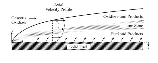
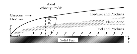
We now turn our attention to a review of the regression rate model developed at UTC by Marxman and his associates. Their model describes the heat transfer pathways within a hybrid motor and leans heavily on the earlier work of Lees [9], who performed a similar analysis in a chemically reactive environment with blowing. The model assumes that the flow is developing along the entire length of the grain (i.e., the boundary layers on either side of the motor have not yet merged at the center-line and a core flow of nearly pure oxidizer exists). Thus, the model does not accurately portray motors whose flow becomes fully developed in the port or is dominated by injector effects over a large region of the head end. The foundational relationship of Marxman’s model consists of an equivalence between the heat transferred from the gas to the wall and the energy absorbed in vaporizing the solid fuel:

$${\dot{Q}}_{\mathrm{w}}={\dot{m}}_{\mathrm{f}}^{″}{h}_v={\rho }_{\mathrm{f}}\dot{r}{h}_v,$$

(1)

where ${\dot{Q}}_{\mathrm{w}}$, ${\dot{m}}_{\mathrm{f}}^{″}$, $h_v$, and ${\rho }_{\mathrm{f}}$ represent the total heat flux at the wall, the fuel mass flux leaving the surface, the effective heat of gasification (which combines the heat of vaporization and melting, the heating of the solid fuel grain, and the heat of reaction associated with polymer degradation), and the fuel density, respectively. Note that the fuel is assumed to pyrolyze and vaporize, as is the case with most polymers, and that Marxman’s model is not accurate for liquefying fuels (such as paraffin wax) that characteristically form a low-viscosity melt layer at the surface. The grain regression rate is represented by $\dot{r}$, in keeping with most other authors, despite some later simplifications that assume a planar configuration. Implicit in the relation specified in Equation (1) is the assumption that there are no heat losses through the grain to the motor casing or outside environment. Experiments and theories have both shown that such conditions provide a reasonable portrayal of normal operations for most hybrid motors, with the thermal waves penetrating only a short distance below the grain surface at moderate regression rates [6]. Next, a more specific expression for the heat transferred from the gas to the wall is given by

$${\dot{Q}}_{\mathrm{c}}=-{\left(\frac{k}{c_p}\frac{\partial h}{\partial y}\right)}_{\mathrm{w}},$$

(2)

where ${\dot{Q}}_{\mathrm{c}}$, k, $c_p$, h, and y represent the convective heat flux (including the effect of partial enthalpies transport by species diffusion), thermal conductivity of the gas, specific heat of the gas, enthalpy of the gas, and normal distance into the flow from the fuel surface, respectively. Here the subscript ‘w’ refers to properties evaluated at the wall. Equation (2) appears as a conductive expression, although it is not explicitly labeled as such in Marxman and Gilbert’s [5] original paper. It should be noted that applying such a simple conductive heat transfer relation to combusting flow implies the assumption that $\mathrm{Le}=\mathrm{Pr}=1$ and that the Reynolds analogy is valid for turbulent flow. As for the radiative component of the total heat flux, it represents a smaller contribution than convection in most hybrids. Whether the effect of radiation is small enough to be safely neglected, as in Equation (2), depends on the propellants and motor operating conditions: Although the polymethyl methacrylate (PMMA)-O${}_2$ systems studied at UTC display a weak radiation dependence, several hybrid motors behave differently. The importance of radiation is discussed at greater length in a later section.

The first of the two major hurdles in describing the heat transfer pathway has now been reached; namely, the challenge of determining the amount of convective heat flux at the wall, based on the known characteristics of the turbulent flow. The Stanton number is introduced, for this purpose, as it represents the ratio of the heat transferred into a fluid to the thermal capacity of that fluid:

$$\mathrm{St}=\frac{{\dot{Q}}_{\mathrm{c}}}{{\rho }_{\mathrm{b}}{u}_{\mathrm{b}}\Delta h},$$

(3)

where the difference in gas-sensible enthalpy $\Delta h$ is evaluated between the flame zone, denoted by a subscript b, and the gas at the wall. In the above, the axial velocity of the burned gas is designated as $u_{\mathrm{b}}$. Writing the wall energy balance, Equation (1), in terms of the Stanton number, we have

$${\rho }_{\mathrm{f}}\dot{r}=\frac{{\dot{Q}}_{\mathrm{c}}}{h_v}=\frac{{\dot{Q}}_{\mathrm{w}}}{h_v}=\mathrm{St}{\rho }_{\mathrm{b}}{u}_{\mathrm{b}}\frac{\Delta h}{h_v},$$

(4)

so that $\dot{Q}$, which is unknown and difficult to estimate directly, is eliminated.

At this juncture, the Reynolds analogy may be invoked to establish an approximate relationship between the unknown heat flux and the better-understood shear stress within the boundary layer. In this process, the Prandtl and Lewis numbers between the wall and the flame zone are taken to be of order unity. It should be noted that, since real hybrids often experience conditions that differ from the idealized assumptions made here, the Chilton–Colburn analogy may replace the Reynolds analogy for cases where $\mathrm{Pr}\ne 1$ or in the presence of an axial pressure gradient. In fact, it may be shown that the difference in the final regression rate relation is rather small when these effects are taken into account (see Marxman [7]). Accordingly, the thermal and molecular diffusion mechanisms associated with the energy and momentum transfers within the boundary layer may be assumed to be driven by similar turbulent mixing processes. Subsequently, the Reynolds analogy may be written as an equivalence between the ratio of the heat flux to the radial gradient of total enthalpy $h_T$ and the ratio of the shear stress $\tau$ to the radial gradient of the axial velocity:

$$-\frac{\dot{Q}}{\partial h_T/\partial y}=\frac{\tau }{\partial u/\partial y}.$$

(5)

This expression may be integrated from the wall to the flame zone, since the object of invoking the analogy is to link properties at these two points. Direct integration yields

$$\frac{{\dot{Q}}_{\mathrm{c}}}{\Delta h_T}=\frac{{\tau }_{\mathrm{w}}}{u_{\mathrm{b}}}.$$

(6)

If no combustion occurs in the low-speed region below the flame, $\Delta h=\Delta h_T$ and dividing by ${\rho }_{\mathrm{b}}{u}_{\mathrm{b}}$ leads to an alternate expression for the Stanton number, in terms of the wall shear stress ${\tau }_{\mathrm{w}}$ or the skin friction coefficient $C_f$, by

$$\mathrm{St}=\frac{{\tau }_{\mathrm{w}}}{{\rho }_{\mathrm{b}}{u}_{\mathrm{b}}^2}=\frac{1}{2}{C}_f\frac{{\rho }_{\mathrm{e}}{u}_{\mathrm{e}}^2}{{\rho }_{\mathrm{b}}{u}_{\mathrm{b}}^2}.$$

(7)

Finally, substituting Equation (7) into Equation (4) enables us to write

$${\rho }_{\mathrm{f}}\dot{r}=\frac{1}{2}{C}_f{\rho }_{\mathrm{e}}{u}_{\mathrm{e}}\frac{u_{\mathrm{e}}}{u_{\mathrm{b}}}\frac{\Delta h}{h_v}.$$

(8)

Note that $\dot{Q}$ has now been replaced in the expression by $C_f$, which is more straightforward to estimate. The first hurdle has been cleared.

Next, the skin friction coefficient may be calculated using a suitable empirical relation. Marxman used the well-known expression for turbulent flow over a flat-plate with no blowing (Schlichting [10]),

$$\frac{C_{f_0}}{2}=0.03{\mathrm{Re}}_x^{-0.2},$$

(9)

where the reference flat-plate value for the skin friction coefficient is given the zero subscript, in order to distinguish it from the value applicable to the combusting flowfield. The local Reynolds number in this expression is given in terms of the freestream properties at the boundary layer edge, denoted here with a subscript ‘e,’ and the axial distance x from the grain leading edge, specifically

$${\mathrm{Re}}_x\equiv \frac{{\rho }_{\mathrm{e}}{u}_{\mathrm{e}}x}{{\mu }_{\mathrm{e}}}.$$

(10)

Making use of this relation entails two principal assumptions: First, that the presence of blowing does not change the nature of the flow so much that a standard value of the friction coefficient modified by a correction factor would be invalidated and, second, that the result for a flat plate will adequately describe the motion in a typical cylindrical and center-perforated grain. The validity of the first assumption largely depends on the complexity or degrees of freedom offered by the correction factor applied. The flat-plate assumption is generally accepted for axially-injected hybrid motors—the grain curvature becomes inconsequential to the analysis in the absence of swirl (i.e., when the motion lacks a significant tangential component). In such configurations, the boundary layer length-scales remain at least one order of magnitude smaller than those associated with the radius of curvature, so that the combustion process may be safely modeled using a flat-plate assumption. The combined effect of both assumptions has been examined in the context of swirl-driven motors by at least one researcher [11].

Substituting the skin friction coefficient expression given by Equation (9) into the energy balance in Equation (8) produces

$${\rho }_{\mathrm{f}}\dot{r}=0.03{\rho }_{\mathrm{e}}{u}_{\mathrm{e}}{\mathrm{Re}}_x^{-0.2}\frac{C_f}{C_{f_0}}\frac{u_{\mathrm{e}}}{u_{\mathrm{b}}}\frac{\Delta h}{h_v}.$$

(11)

All that remains is to find a “blowing correction,” $C_f/C_{f_0}=\mathrm{St}/{\mathrm{St}}_0$, that will account for the difference in heat flux between the combusting (i.e., blowing) and non-combusting cases. For convenience, the blowing parameter B is first defined as

$$B\equiv \frac{u_{\mathrm{e}}}{u_{\mathrm{b}}}\frac{\Delta h}{h_v},$$

(12)

so that

$${\rho }_f\dot{r}=0.03{\rho }_{\mathrm{e}}{u}_{\mathrm{e}}\frac{C_f}{C_{f_0}}{\mathrm{Re}}_x^{-0.2}B.$$

(13)

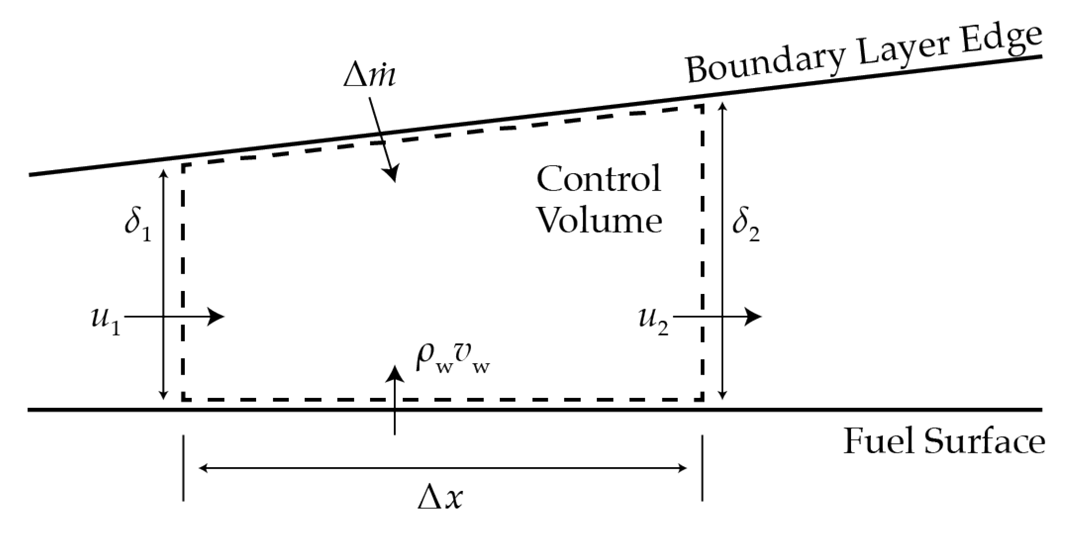
The blowing parameter, thus, appears as a thermochemical parameter, which depends on the flame location within the boundary layer and which can be specified for a particular propellant combination. While it is clear that the heat of gasification and difference in enthalpies are determined by the propellants and mixture ratio, the dependence of the velocity ratio $u_{\mathrm{e}}/u_{\mathrm{b}}$, which is closely linked to the flame height, on these same parameters is less evident. This dependence may be verified by integrating the oxidizer and fuel mass fluxes through a pair of control volumes separated by the flame zone and comparing the results to the integral momentum equation. One obtains

$$\frac{u_{\mathrm{e}}}{u_{\mathrm{b}}}=\frac{K_{{\mathrm{ox}}_{{}_{\mathrm{e}}}}+\left(\mathrm{O}/\mathrm{F}+K_{{\mathrm{ox}}_{{}_{\mathrm{e}}}}\right)\left(\Delta h/h_v\right)}{\left(\mathrm{O}/\mathrm{F}\right)\left(\Delta h/h_v\right)},$$

(14)

where $K_{{\mathrm{ox}}_{{}_{\mathrm{e}}}}$ is the oxidizer concentration in the free stream and O/F is the local oxidizer to fuel ratio at the flame [6]. For the equi-diffusive case, the blowing parameter also proves to be a similarity parameter of the boundary layer. In other words, when $\mathrm{Le}=\mathrm{Pr}=1$ and $B=\mathrm{const}.$, the velocity, species concentration, and enthalpy profiles become similar everywhere [2,6]. In a follow-up paper, Marxman [7] derived the following expression for the blowing correction

$$\frac{C_f}{C_{f_0}}={\left[\frac{ln(1+B)}{B}\right]}^{0.8}{\left[\frac{1+\frac{13}{10}B+\frac{4}{11}{B}^2}{(1+B){(1+\frac{1}{2}B)}^2}\right]}^{0.2},$$

(15)

which he simplified, using curve fitting, into

$$\frac{C_f}{C_{f_0}}=1.2B^{-0.77}.$$

(16)

Much academic debate has surrounded the proper representation of the blowing correction. In his original presentation, Marxman [7] acknowledged the form derived in Lees [9] using thin-film theory; particularly,

$$\frac{C_f}{C_{f_0}}=\frac{ln(1+B)}{B}.$$

(17)

Marxman concluded that, since mass addition is discounted in the construction of Equation (17), it can only be expected to produce reasonable results for low values of the blowing parameter B. Marxman [7] then derived the equations most often used in the context of hybrids—namely, Equations (15) and (16)—using Prandtl’s mixing length hypothesis combined with von Kármán’s momentum integral analysis. 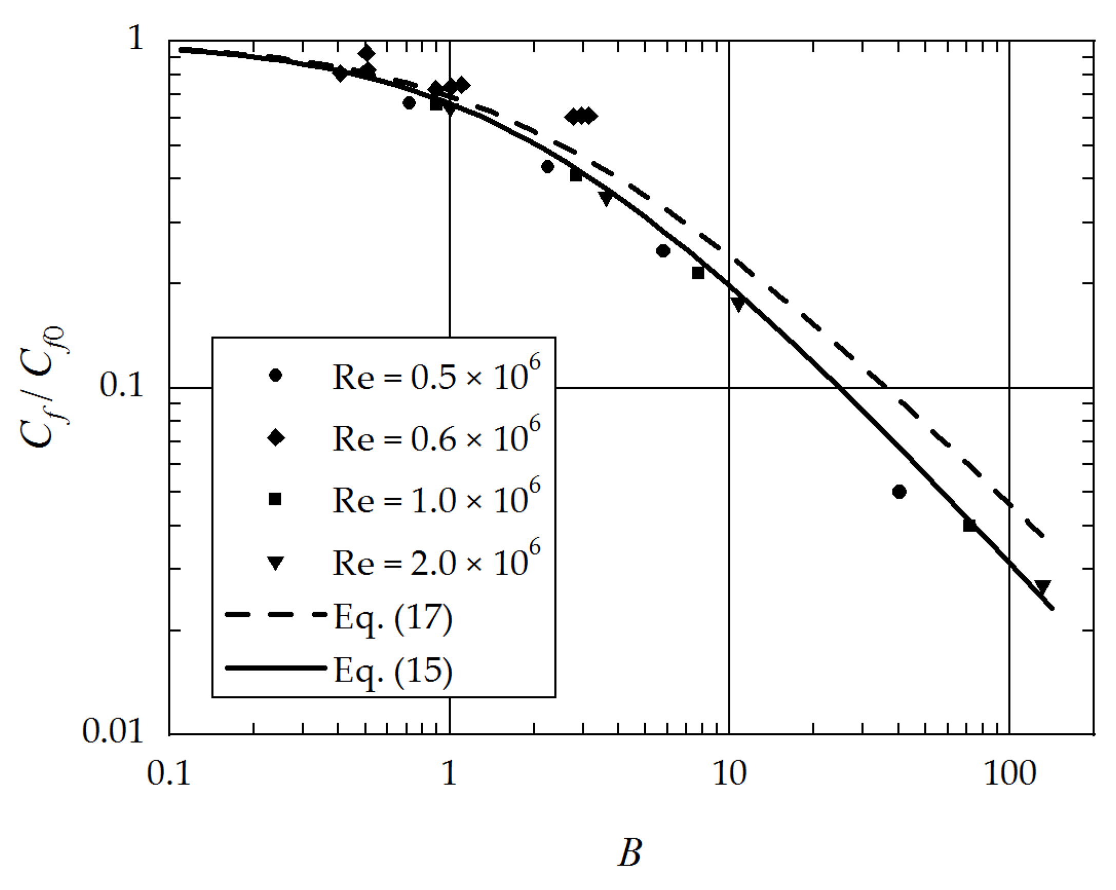Details of this derivation may be found in Appendix A. These expressions lead to better agreement with experiments at high mass injection rates. The improvement in accuracy when moving from Equation (17) to Equation (15) is illustrated in Figure 2 using the experimental data reported by Mickley and Davis [12] as well as Tewfick [13].

A decade later, Lengelle [14] revisited some of Marxman’s assumptions on eddy diffusivity and developed a modified form of the blowing correction. Both derivations were later shown to display inconsistencies with experimental measurements, as well as an exact solution developed by Karabeyoglu [15] under similar conditions. Specifically, Marxman’s expression for the skin friction coefficient did not reduce to the accepted value in the absence of blowing, although his analysis yielded a blowing correction trend that stood in better agreement with experimental measurements. Meanwhile, Lengelle’s expressions fell closer to the analytical solution for skin friction but overestimated the blowing correction when compared to experiments. Based on this realization, Karabeyoglu set about deriving a new expression that did not rely on the same assumptions drawn from Prandtl’s mixing length hypothesis. He arrived at an expression for the blowing correction that was nearly identical to Equation (15) of Marxman [7], albeit with a more self-consistent expression for the skin friction coefficient. In the end, Karabeyoglu suggested the use of a simplified exponential expression and pointed out that Altman [4] had already shown that a simple power-law relation remained a more accurate representation than Equation (16) over a practical range of interest. This relation is simply

$$\frac{C_f}{C_{f_0}}=B^{-0.68}.$$

(18)

Nonetheless, by substituting Marxman’s simplified blowing correction, Equation (16), into the regression rate expression given by Equation (13), one gets

$${\rho }_{\mathrm{f}}\dot{r}=0.036{\rho }_{\mathrm{e}}{u}_{\mathrm{e}}{\mathrm{Re}}_x^{-0.2}{B}^{0.23},$$

(19)

or, in terms of the mass flux $G\equiv {\rho }_{\mathrm{e}}{u}_{\mathrm{e}}$,

$${\rho }_{\mathrm{f}}\dot{r}=0.036G{\left(\frac{Gx}{{\mu }_{\mathrm{e}}}\right)}^{-0.2}{B}^{0.23}.$$

(20)

We, thus, arrive at Marxman’s form of the local regression rate in the absence of radiation, although a more commonly seen result may be obtained by consolidating the constant properties in Equation (20) to produce the compact relation

$$\dot{r}=A{G}^{0.8}{x}^{-0.2},$$

(21)

where A remains approximately invariant for a given propellant. Note that the space-time averaged equivalent of Equation (21) is often used by researchers reporting experimental measurements, specifically,

$$\dot{r}=m{G}^n.$$

(22)

In the above, combining B with the other constants is justified by noting that, as long as $\Delta h/h_v$ does not change with ${\mathrm{Re}}_x$, then the distribution of the regression rate will be such that B remains spatially uniform [6]. Even when this is not strictly the case, B is expected to display very small variations along the length of the grain. The small exponent of B further ensures that even large changes in $\Delta h$ or $h_v$ will have negligible effects on the overall regression rate. Another consequence of this relation is that values of B calculated for one propellant can be extended, with reasonable accuracy, to other propellants, so long as they share similar compositions and conditions that justify ignoring radiation effects. The relation also suggests that any possible oxidative reactions at the fuel surface that alter $\Delta h/h_v$ from its idealized value will have a minor effect on the regression rate (see the reply to Rosner’s comment in [7] for context and elaboration on the significance of this implication).

Before leaving this subject, it may be helpful to reflect on several regression rate characteristics that may be gleaned from Equation (20). First and foremost, one notes the absence of any pressure dependence in the expression for $\dot{r}$. While this behavior remains contingent on discarding radiative effects, an assumption which will be later examined in more depth, it proves to be surprisingly accurate for many systems. Physically, the lack of a pressure dependence may be attributed to the diffusion-flame burning response, which stands as the single most defining characteristic for hybrids. In fact, one may argue that a mass flux-controlled motor offers distinct advantages over a pressure-dependent solid motor. Designers are now permitted more freedom in choosing a motor operating pressure which helps to achieve a desired target performance or meet certain safety requirements, which can be particularly useful in research and adoption in academic settings. Another feature captured in Equation (20) consists of the axial variation in regression rate, which encompasses both a positive correlation with axial distance as fuel injection increases the local mass flux (i.e., the flux increases at locations further downstream as more fuel mass is added to the flow), and a negative correlation with axial distance, which may be associated with boundary layer growth and the corresponding decrease in the skin friction coefficient and, thus, the heat flux, in conformance with the Reynolds analogy. These competing factors result in an equilibrium location for the minimum regression rate that shifts downstream with the passage of time.

4. Radiation

Up to this point, several pressure-dependent mechanisms that can influence the regression rate in a hybrid motor have been ignored. Foremost among them is radiative heat transfer, which can contribute significantly to the overall fuel regression behavior, depending on the motor operating conditions and fuel composition. Although some researchers have found that the purely convective heat transport equations remain the most reliable for hydrocarbon fuels [16], Marxman and Gilbert recognized the potential importance of radiative heat transfer immediately and included a crude treatment of the subject in their initial investigation [5], specifically by adding a grey-body radiation term to the regression rate expression described above. They wrote

$${\rho }_{\mathrm{f}}\dot{r}=0.036G{\left(\frac{Gx}{{\mu }_{\mathrm{e}}}\right)}^{-0.2}{B}^{0.23}+\frac{\sigma {ϵ}_{\mathrm{w}}\left({ϵ}_{\mathrm{g}}{T}_{\mathrm{b}}^4-T_{\mathrm{w}}^4\right)}{h_v},$$

(23)

where ${ϵ}_{\mathrm{g}}$ denotes the emissivity of the gas, while ${ϵ}_{\mathrm{w}}$ refers to the emissivity of the wall and $\sigma$ stands for the Stefan-Boltzmann constant. However, since this expression neglects the strong coupling between radiation and the blocking effect, it does not agree well with experiments. Marxman et al. [6] addressed this coupling by representing the radiative contribution in two equivalent ways: On one hand, applying a correction factor to the blowing parameter in Equation (20) results in the modifier ${(B_{\mathrm{rad}}/B)}^{0.23}$ that accounts for the entire effect of radiation in one simple term:

$${\rho }_{\mathrm{f}}\dot{r}=0.036G{\left(\frac{Gx}{{\mu }_{\mathrm{e}}}\right)}^{-0.2}{B}^{0.23}{\left(\frac{B_{\mathrm{rad}}}{B}\right)}^{0.23}.$$

(24)

On the other hand, the effect of radiation may be included more explicitly by recognizing that, to account for coupling, Equation (23) need only be adjusted by modifying the blowing correction in the convective term, such that

$${\rho }_{\mathrm{f}}{h}_v\dot{r}={\dot{Q}}_{\mathrm{c}}{\left(\frac{B_{\mathrm{rad}}}{B}\right)}^{-0.77}+{\dot{Q}}_{\mathrm{rad}},$$

(25)

where

$${\dot{Q}}_{\mathrm{c}}=0.036G{h}_{v}R{e}_x^{-0.2}{B}^{0.23}\mathrm{and}{\dot{Q}}_{\mathrm{rad}}=\sigma {ϵ}_{\mathrm{w}}\left({ϵ}_{\mathrm{g}}{T}_{\mathrm{b}}^4-T_{\mathrm{w}}^4\right).$$

Combining Equations (24) and (25) leads to the correction factor

$$\frac{B_{\mathrm{rad}}}{B}=1+\frac{{\dot{Q}}_{\mathrm{rad}}}{{\dot{Q}}_{\mathrm{c}}}{\left(\frac{B_{\mathrm{rad}}}{B}\right)}^{0.77}.$$

(26)

Although this equation cannot be solved explicitly, its solution can be approximated adequately using an expression provided in [6],

$$\frac{B_{\mathrm{rad}}}{B}=exp\left(\frac{1.3{\dot{Q}}_{\mathrm{rad}}}{{\dot{Q}}_{\mathrm{c}}}\right),$$

(27)

which, when substituted back into Equation (25), yields a simple, closed-form approximation, specifically

$${\rho }_{\mathrm{f}}\dot{r}=\left[{\dot{Q}}_{\mathrm{c}}exp\left(-{\dot{Q}}_{\mathrm{rad}}/{\dot{Q}}_{\mathrm{c}}\right)+{\dot{Q}}_{\mathrm{rad}}\right]/h_v.$$

(28)

If more accuracy is desired, a three-term asymptotic approximation may be used; namely,

$$\frac{B_{\mathrm{rad}}}{B}=exp\left[\left(\frac{{\dot{Q}}_{\mathrm{rad}}}{{\dot{Q}}_{\mathrm{c}}}\right)+0.27{\left(\frac{{\dot{Q}}_{\mathrm{rad}}}{{\dot{Q}}_{\mathrm{c}}}\right)}^2+0.06768{\left(\frac{{\dot{Q}}_{\mathrm{rad}}}{{\dot{Q}}_{\mathrm{c}}}\right)}^3\right].$$

(29)

Equation (29) proves to be in closer agreement with the exact solution than Equation (27). If simplicity is desired, an alternate one-term approximation may be used that remains more accurate than Equation (27) as long as radiation contributes no more than two-thirds of the convective heat flux. This expression is

$$\frac{B_{\mathrm{rad}}}{B}=exp\left(\frac{1.13727{\dot{Q}}_{\mathrm{rad}}}{{\dot{Q}}_{\mathrm{c}}}\right).$$

(30)

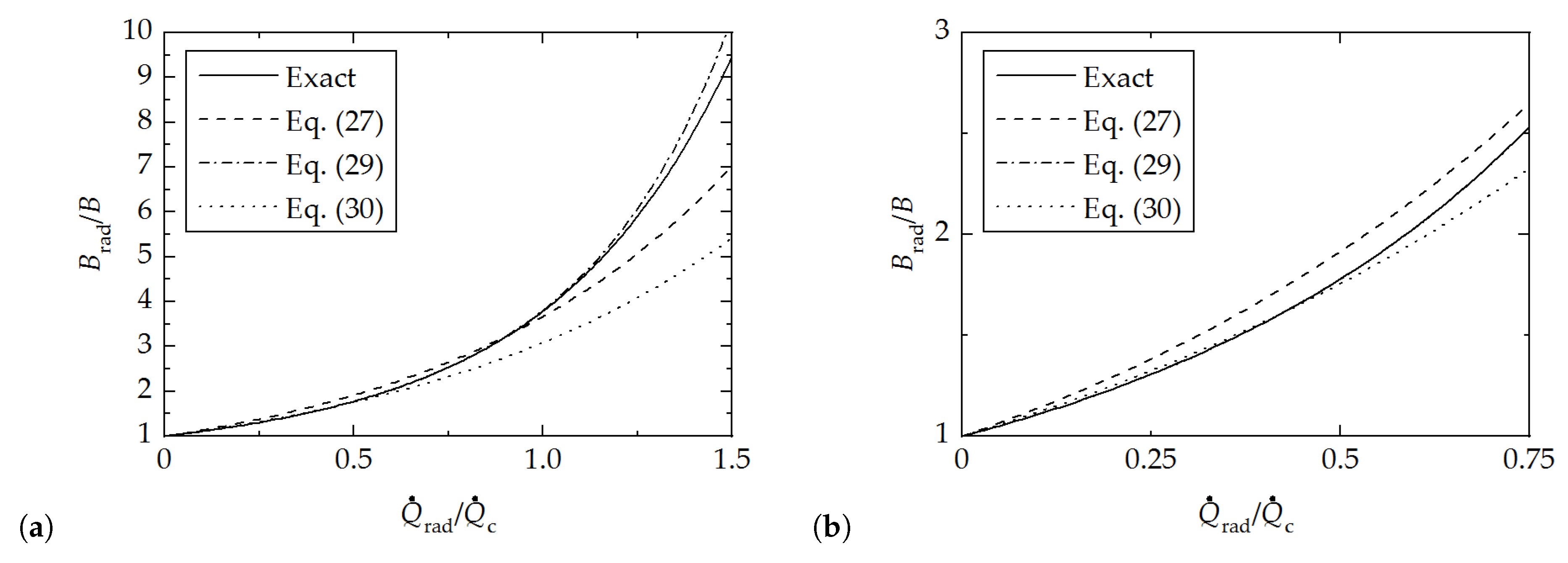
In the interest of clarity, the different solutions for the radiation correction are plotted in Figure 3 along with the numerical solution to Equation (26). Note that each approximation has its own merits: While being the least accurate, Equation (27) remains adequate over the entire domain and results in unitary coefficients, as per Equation (28). Equation (29) remains the most accurate over the entire domain, and Equation (30) remains nearly indiscernible from the numerical solution for smaller radiative contributions while remaining simple to apply, as long as ${\dot{Q}}_{\mathrm{rad}}/{\dot{Q}}_{\mathrm{c}}\le 2/3$. All these expressions, however, correspond to Marxman’s curve-fitted model for the blowing correction given by Equation (16). Naturally, a different form of $C_f/C_{f_0}$ would lead to a slightly dissimilar set of expressions for $B_{\mathrm{rad}}/B$.

For systems with low values of ${\dot{Q}}_{\mathrm{rad}}/{\dot{Q}}_{\mathrm{c}}$, Marxman et al. [6] note that the tradeoff between the new terms in Equation (28) is “nearly exact, and $\dot{r}$ can be calculated with little error by using ${\dot{Q}}_{\mathrm{c}}$ alone”. If ${\dot{Q}}_{\mathrm{rad}}={\dot{Q}}_{\mathrm{c}}$, then Equation (28) predicts that approximately three quarters of the heat actually transferred to the wall will be due to radiation but that $\dot{r}$ will be only 35% higher than the case with no radiation. While useful for illustrative purposes, this result should be treated with care: If the majority of heat transferred is radiative, the dependencies on geometry will no longer be the same as those already considered for the purely convective case. Furthermore, the accuracy of Equation (28) degrades rapidly once radiative heat flux overtakes that due to convection, as evidenced in Figure 3.

In a paper published three years later, Marxman [17] added further insight into the radiation problem. He proceeded to classify three general situations where radiation becomes appreciable:

• Grains containing particles that react incompletely in the flame to the extent of producing solid or liquid products (e.g., metallized fuels);
• grains that naturally produce solid or liquid products beyond the flame (e.g., carbon-heavy or sooty fuels); and
• propellants whose gas-phase combustion products produce appreciable radiation.

All three cases may be described by similar expressions, with the primary difference being in how the number density of radiating particles must be treated. Furthermore, the heat transfer in all three cases becomes dependent on the chamber pressure through the particle number density. Marxman noted that, for the first two cases, the most appropriate effective optical path length will likely be the distance from the surface to the flame zone, since the particle phase absorptivity will be high beyond that point. For the third case, he posited that the optical path length will depend on a characteristic chamber dimension, such as the diameter. 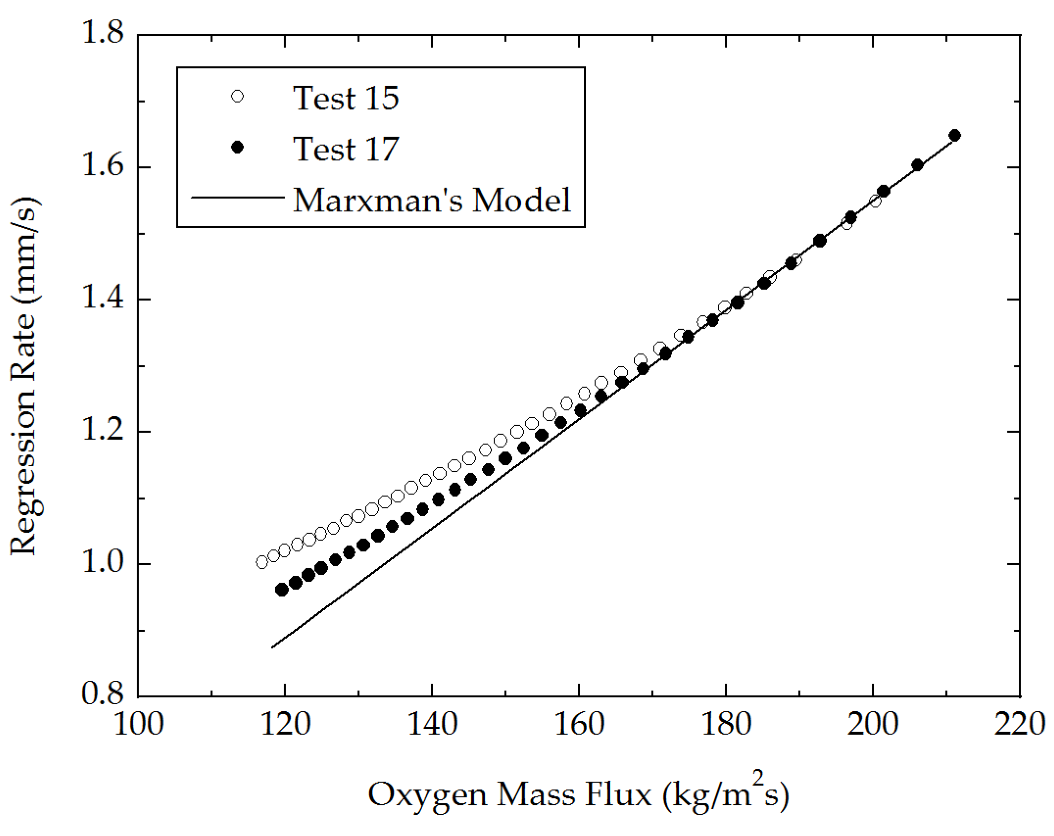Although Marxman’s group worked primarily with PMMA-O${}_2$ systems with negligible radiation, other experiments with hydroxyl-terminated polybutadiene (HTPB) grains have confirmed that radiation effects indeed become significant at higher motor pressures and lower oxidizer mass fluxes. To further illustrate this behavior, Figure 4 is used to display the radiation dependence obtained in one such investigation by Chiaverini et al. [18]. Note that test 15 was performed at a higher pressure than test 17 and thus displayed a stronger variance from the values predicted by Marxman’s diffusion-limited, convection-driven model. Both data sets agree with the theory at higher mass fluxes, where convection dominates the heat transfer process to the extent of justifying the use of a non-radiative model.

5. Other Non-Ideal Considerations

In his 1965 paper, Marxman [7] provided a derivation for the regression rate, which parallels that of Marxman et al. [6], just described in detail, where the fundamental work of Lees [9] was revisited by relaxing the assumption that $\mathrm{Pr}=1$ to that of $\mathrm{Pr}=$ const. In this case, the thermochemical parameter B becomes different from the aerodynamic similarity parameter $B^{\prime }$, according to

$$B=B^{\prime }{\mathrm{Pr}}^{0.67};$$

(31)

at the outset, Equation (20) becomes

$${\rho }_{\mathrm{f}}\dot{r}=0.036G{\left(\frac{Gx}{{\mu }_{\mathrm{e}}}\right)}^{-0.2}{B}^{0.23}{\mathrm{Pr}}^{-0.15}.$$

(32)

As $\mathrm{Pr}$ is close to unity for most gases, even at high temperatures, the effect of ${\mathrm{Pr}}^{-0.15}$ remains sufficiently small to render the correction unnecessary in most cases. The same study by Marxman [7] separately addressed the assumption of uniform gas density between the flame and the wall by using a Howarth–Dorodnitsyn variable transformation to relate the actual, variable-property turbulent boundary layer to an equivalent incompressible boundary layer, through

$${\rho }_{\mathrm{f}}\dot{r}=0.036G{\left(\frac{{\rho }_0}{{\rho }_{\mathrm{e}}}\right)}^{0.6}{\left(\frac{Gx}{{\mu }_{\mathrm{e}}}\right)}^{-0.2}{B}^{0.23},$$

(33)

where the reference state ratio ${\rho }_0/{\rho }_{\mathrm{e}}$ is determined from a semi-empirical relation, described in terms of previously defined parameters and the boundary layer thickness $\delta$, which must be measured experimentally. Due to the added complexity, the variable-density correction is seldom used.

6. Kinetics-Limited Models

The importance of kinetics, both homogeneous and heterogeneous, has long been the subject of debate. As previously mentioned, Marxman [7] received criticism for neglecting heterogeneous surface reactions but argued that the effects of reactions below the flame on the values of $\Delta h$ and $h_v$ remained of secondary importance. However, several researchers have developed models and correlations in which kinetics played a major role. A selection of these, loosely grouped according to their dominant physical mechanism, is overviewed here as a starting point for further reading. This cursory coverage is not intended to be comprehensive, in scope nor in detail.

The first group of researchers are those who were primarily concerned with gas-phase kinetics. For example, Wooldridge et al. [19] studied pressure sensitivity at low pressures in an attempt to characterize the stability characteristics of hybrids. This effort entailed the development of an analytical expression for the regression rate as a function of several kinetic parameters and length-scales. Miller [20] developed a model that incorporated both the fuel diffusion rate and the chemical reaction rates, which he used to successfully correlate data taken by Smoot and Price [21,22,23]. Kosdon and Williams [24] later noted that Miller’s analysis was only applicable to systems with low pressure and moderate oxidizer fluxes and derived a new expression that incorporated a flame zone of finite thickness. Wooldridge and Muzzy [25] examined the effects of scaling and pressure on motor performance in the context of throttling. In his 1972 article, [26] pointed out that even simple PMMA-O${}_2$ motors behaved differently at low pressures and that as the motor approached a flooding condition, combustion likely became kinetically-limited. By reviewing existing test data, he formed an explicitly pressure-dependent correlation which could be likened to that of Wooldridge et al. [19], specifically

$$\dot{r}\propto P^{0.5}{G}^{0.3}{x}^{-0.2}.$$

(34)

Another group of researchers focused more on heterogeneous surface reactions as the source of kinetics dependence. Smoot and Price [21,22,23] performed numerous tests using a slab burner and found that, above a threshold value of G, the regression rate became nearly independent of G and instead varied with P and the oxidizer composition. These researchers defined a low mass flux regime where the normal $G^{0.8}$ dependence held, an intermediate mass flux regime where both P and G played a role, and a third regime at very high mass fluxes where the regression rate varied with pressure, as in the case of a solid rocket propellant; namely,

$$\dot{r}\propto P^n.$$

(35)

Kumar and Stickler [27] cited discrepancies in hybrid test data and pyrolysis tests in an inert environment for PMMA to support their hypothesis that heterogeneous reactions must play a significant role in regression rate estimations. They additionally argued that the gas-phase kinetics could not be sufficiently slow to play a consequential role. They developed a correlation that normalized the regression rate by its maximum value before pressure effects appeared in a manner to make it possible to predict whether a particular set of conditions was kinetically or diffusively limited, in addition to successfully matching experimental data. More recently, Favaro et al. [28] performed experiments designed to illuminate the role of heterogeneous reactions, thus leading to the development of a semi-empirical model.

Despite the number of investigations into kinetically-limited operating regimes, Marxman’s model and the assumptions that it prescribed have become the de facto standard for normal applications. This does not mean, however, that experts in the field have reached a definitive agreement on how to properly model regression in all situations. While modern computational studies are increasingly contributing to the understanding of diffusion-limited combustion in ways that may be less restrictive, Marxman’s model is still commonly used to guide the design of hybrid systems and as a basis for the development of further analytical treatments of geometrically or thermophysically more complex hybrids, such as those incorporating swirl or liquefying fuels.

7. Summary

The key points that would be useful to remember by those interested in hybrid rocket regression rate modeling and its practical implementation may be summarized as follows:

• Marxman’s theory is based on the assumption that the diffusion of oxidizer and fuel into the flame establishes the rate-limiting process in hybrid combustion and leads to adequate predictions at the moderate pressures and mass fluxes that accompany the steady-state operation of most hybrid motors.
• For classical, non-metallized hybrids, the fuel regression rate depends on $G^{0.8}$, but not on pressure.
• Radiation appears as a secondary correction, but should not be neglected at low mass fluxes or for metallized or other heavily sooting fuels.
• Most of the improvements to the initial diffusion-limited model, besides radiation treatment, lead to rather small corrections to the end result and may typically be ignored.
• Numerous alternate regression rate models have been formulated to be more accurate for kinetically-limited operating conditions.

For those seeking more information or a deeper understanding of regression rate models, the seminal reviews of the subject by Netzer [2] and Chiaverini [3] are suggested, along with Marxman’s 1965 paper [7]. Improvements and extensions to regression rate models in novel and emerging hybrid configurations continue today and it is hoped that this cursory review will prove useful to researchers entering the field and seeking to describe the internal workings of these new and exciting hybrid motors.

References

1. Altman, D. Hybrid Rocket Development History. In Proceedings of the 27th AIAA/ASME/SAE/ASEE Joint Propulsion Conference and Exhibit, Sacramento, CA, USA, 24–26 June 1991. [Google Scholar] [CrossRef]
2. Netzer, D.W. Hybrid Rocket Internal Ballistics; Technical Report; Chemical Propulsion Information Agency: Silver Spring, MD, USA, 1972. [Google Scholar]
3. Chiaverini, M.J. Review of Solid-Fuel Regression Rate Behavior in Classical and Nonclassical Hybrid Rocket Motors. In Fundamentals of Hybrid Rocket Combustion and Propulsion; Chiaverini, M.J., Kuo, K.K., Eds.; American Institute of Aeronautics and Astronautics: Reston, VA, USA, 2007; Chapter 2; Volume 218, pp. 37–126. [Google Scholar]
4. Altman, D.; Humble, R. Space Propulsion Analysis and Design; McGraw-Hill Book Company: New York, NY, USA, 1995; Chapter 7; pp. 365–442. [Google Scholar]
5. Marxman, G.; Gilbert, M. Turbulent Boundary Layer Combustion in the Hybrid Rocket. Ninth Symp. Combust. 1963, 9, 371–383. [Google Scholar] [CrossRef]
6. Marxman, G.A.; Wooldridge, C.E.; Muzzy, R.J. Fundamentals of Hybrid Boundary Layer Combustion. Prog. Aeronaut. Astronaut. 1964, 15, 485–522. [Google Scholar] [CrossRef]
7. Marxman, G.A. Combustion in the Turbulent Boundary Layer on a Vaporizing Surface. Tenth Symp. Combust. 1965, 10, 1337–1349. [Google Scholar] [CrossRef]
8. Marxman, G.A.; Wooldridge, C.E. Research on the Combustion Mechanism of Hybrid Rockets. In Advances in Tactical Rocket Propulsion, AGARD Conference Proceedings No. 1; Technivisions Services: London, UK, 1968; pp. 421–477. [Google Scholar]
9. Lees, L. Convective Heat Transfer with Mass Addition and Chemical Reactions. In Combustion and Propulsion–Third AGARD Colloquium: Noise-Shock Tubes-Magnetic Effects-Instability and Mixing; Pergamon Press: New York, NY, USA, 1958; p. 451. [Google Scholar]
10. Schlichting, H. Boundary-Layer Theory, 7th ed.; Kestin, J., Translator; McGraw-Hill Book Company: New York, NY, USA, 1979. [Google Scholar]
11. Knuth, W.; Chiaverini, M.; Gramer, D.; Sauer, J. Solid-Fuel Regression Rate and Combustion Behavior of Vortex Hybrid Rocket Engines. In Proceedings of the 35th AIAA/ASME/SAE/ASEE Joint Propulsion Conference and Exhibit, Los Angeles, CA, USA, 20–24 June 1999. [Google Scholar] [CrossRef]
12. Mickley, H.S.; Davis, R.S. Momentum Transfer for Flow Over a Flat Plate with Blowing; Technical Report, NACA TN-4017; National Advisory Committee for Aeronautics: Washington, DC, USA, 1957.
13. Tewfick, O.E. Some Characteristics of the Turbulent Boundary Layer with Air Injection. AIAA J. 1963, 1, 1306–1312. [Google Scholar] [CrossRef]
14. Lengelle, G. Model Describing the Erosive Combustion and Velocity Response of Composite Propellants. AIAA J. 1975, 13, 315–322. [Google Scholar] [CrossRef]
15. Karabeyoglu, M.A. Transient Combustion in Hybrid Rockets. Ph.D. Thesis, Stanford University, Stanford, CA, USA, 1998. [Google Scholar]
16. Estey, P.; Altman, D.; McFarlane, J. An Evaluation of Scaling Effects for Hybrid Rocket Motors. In Proceedings of the 27th AIAA/ASME/SAE/ASEE Joint Propulsion Conference, Sacramento, CA, USA, 24–26 June 1991. [Google Scholar] [CrossRef]
17. Marxman, G.A. Boundary Layer Combustion in Propulsion. Elev. Symp. Combust. 1967, 11, 269–289. [Google Scholar] [CrossRef]
18. Chiaverini, M.J.; Serin, N.; Johnson, D.K.; Lu, Y.C.; Kuo, K.K.; Risha, G.A. Regression Rate Behavior of Hybrid Rocket Solid Fuels. J. Propuls. Power 2000, 16, 125–132. [Google Scholar] [CrossRef]
19. Wooldridge, C.E.; Marxman, G.A.; Kier, R.J. Investigation of Combustion Instability in Hybrid Rockets; Technical Report; National Aeronautics and Space Administration, Langley Research Center: Hampton, VA, USA, 1969.
20. Miller, E. Hybrid Rocket Combustion Regression Rate Model. AIAA J. 1966, 4, 752–753. [Google Scholar] [CrossRef]
21. Smoot, L.D.; Price, C.F. Regression Rates of Nonmetalized Hybrid Fuel Systems. AIAA J. 1965, 3, 1408–1413. [Google Scholar] [CrossRef]
22. Smoot, L.D.; Price, C.F. Regression Rates of Metalized Hybrid Fuel Systems. AIAA J. 1966, 4, 910–915. [Google Scholar] [CrossRef]
23. Smoot, L.D.; Price, C.F. Pressure Dependence of Hybrid Fuel Regression Rates. AIAA J. 1966, 5, 102–106. [Google Scholar] [CrossRef]
24. Kosdon, F.J.; Williams, F.A. Pressure Dependence of Nonmetalized Hybrid Fuel Regression Rates. AIAA J. 1967, 5, 774–778. [Google Scholar] [CrossRef]
25. Wooldridge, C.E.; Muzzy, R.J. Internal Ballistic Considerations in Hybrid Rocket Design. J. Spacecr. 1967, 4, 255–262. [Google Scholar] [CrossRef]
26. Muzzy, R.J. Applied Hybrid Combustion Theory. In Proceedings of the 8th Joint Propulsion Specialist Conference, New Orleans, LA, USA, 29 November–1 December 1972. [Google Scholar] [CrossRef]
27. Kumar, R.N.; Stickler, D.B. Polymer-Degradation Theory of Pressure-Sensitive Hybrid Combustion. Thirteen. Symp. Combust. 1971, 13, 1059–1072. [Google Scholar] [CrossRef]
28. Favaro, F.M.; Sirignano, W.A.; Manzoni, M.; DeLuca, L.T. Solid-Fuel Regression Rate Modeling for Hybrid Rockets. J. Propuls. Power 2013, 29, 205–215. [Google Scholar] [CrossRef] [Green Version]
Figure 1. Illustrative sketch of the diffusion-limited combustion process in hybrid rockets.
Aerospace 06 00075 g001
Figure 2. Comparison of blowing correction formulations expressed over a range of blowing parameters at several Reynolds numbers. Data taken from [12,13].
Aerospace 06 00075 g002
Figure 3. Comparison of different expressions for the radiation correction shown (a) over a wide range of heat flux ratios, and (b) over a more practical range.
Aerospace 06 00075 g003
Figure 4. Effect of thermal radiation on hydroxyl-terminated polybutadiene (HTPB) regression-rate behavior. Data taken from [18].
Aerospace 06 00075 g004