1. Introduction
The development of aircrafts is driven by a complex business-to-business market, in which suppliers and sub-suppliers need to work with a wide variety of design solutions in order to be adaptive to requirement changes from the OEMs (original equipment manufacturers) [
1].
In the early stages of development, aero-engine manufacturers need to quickly evaluate the feasibility of a large number of design variants to give a rapid response to OEMs in regards to potential performance quality, producibility, and component cost [
2,
3]. Established approaches begin by parametrizing component concept and setting a large design space defined by a broad number of design parameters [
4]. Multidisciplinary optimization in combination with modelling and simulation techniques are then employed to find optimal designs to fulfil high performance requirements such as aerodynamics, extreme temperatures, or safety aspects [
5,
6]. While designs are principally optimized upon component performance, producibility aspects have been considered lately [
7,
8]. However, producibility is also an important constraint to the design space because all manufactured and assembled products are afflicted by variation [
9]. Geometrical variation at a part level can propagate and accumulate throughout the assembly process, resulting in products that do not fulfil assembly, functional, or esthetical conditions.
In the context of assembled products, Söderberg et al. [
10] proposes virtual geometry assurance as a process to foresee geometrical variation from early design stages. Virtual geometry assurance is a set of activities and tools needed to analyse and control the effect of geometrical variation with the use of variation simulation and probabilistic design practices, which allows giving an early response to the OEMs concerning the assembly feasibility and robustness of the component design.
In the last decade, a common approach to the manufacture of aero-engine components has been the fabrication of small parts that are joined together into the final component by employing fusion welding [
11]. For this type of application, laser beam welding (LBW) has played an integral role. LBW is a high energy density beam welding method, which has lately been considered as a promising alternative to the conventional arc welding methods [
12,
13]. This welding method produces welds with high depth-to-width aspect ratios, small heat affected zones, and reduced distortion due to the heat source being a high-energy density beam. Thus, it is an advantageous solution to welding nickel-based super alloy components [
12]. When it comes to weld titanium alloy components, a competitive technology to laser welding is friction stir welding (FSW). FSW is a solid-state joining process that produces a joint without melting the workpiece material. The absence of melting enables very low welding temperatures. As a consequence, mechanical distortion is nearly reduced and the heat affected zone is minimal [
14]. The surface finish quality also increases considerably according to Nandan et al. [
15].
Nevertheless, to perform variation simulation of a welded component, Pahkamma et al. [
16] stated that besides assembly variation, it is necessary to also model the joining process because of the combinatory effect between part variation, assembly variation, and welding deformation. However, modelling welding processes is not an easy task because it involves the interaction of complex thermal, mechanical, and metallurgical phenomena [
17]. In addition, distortion and geometrical variation are not the only characteristics determining the final weld quality. In aerospace applications, weld quality criteria also include weld bead geometry, microstructure, metallurgical discontinuities, and residual stresses [
18]. Therefore, current needs in the field of virtual geometry assurance rely on the capacity of evaluating in a virtual asset whether certain design geometries and parameters can be welded to specific weld quality levels in order to ensure component functionality.
The quality of a welded aero-component can be affected by multiple factors such as welding process parameters and set-up, materials composition, weld joint design, fixture design, product form division, and product geometry [
19,
20]. The interaction of product geometry and welding process causes welding engineers to struggle because they need to find a new optimal set of process parameters for every new component geometry and material to produces a good welded joint.
In the literature, studies can be found that use design of experiments (DOE) and other statistical and numerical approaches to predict and optimize weld quality for different welding methods [
14,
21,
22,
23,
24,
25,
26,
27,
28]. Nevertheless, few studies can be found that optimize the interaction of product geometry and welding process. For example, Casalino et al. [
27] employs neural networks, including joint thickness, as a parameter to predict weld bead geometry. Caiazzo et al. [
24] emphasized that understanding the effect of laser beam incident angle is required for real application in commercial turbine engines. However, the majority of the studies only include conventional welding process parameters such as power and speed in the optimization.
In addition, these welding–DOE studies are performed via physical experiments. The lack of virtual analysis for welding producibility makes the design evaluation longer and more costly when compared with other disciplines such as aerodynamics that have a strong simulation capability. The evaluation time and cost increment even more as more parameters are considered in the DOE. As a consequence, less parameter combinations are physically tested and less information is gained.
Scope and Structure of the Paper
To rapidly evaluate the welding producibility of all geometrical variants considered within the design space, and to be able to gain more welding capability information, there is a need to incorporate virtual approaches that investigate and optimize potential combinations of design and welding parameters. The objective of this study is to propose a method that combines DOE techniques with welding simulation. The use of DOE techniques will allow exploring a big part of the design space, formed by selected design and welding parameters, requiring a minimal number of experiments. Welding simulations will be conducted as virtual experiments to shorten the evaluation time. The aim is to be able to quickly evaluate the effect of the different product geometries on weld quality during early phases of the multidisciplinary design of aerospace components. In this manner, a rapid answer can be provided to the OEM about the design and manufacture feasibility of a component variant.
The virtual and design of experiment method is presented in the Material and Methods section of this article. First, a brief description of the method steps is given. Further on, an industrial case study is employed to give a more detailed explanation of each of the steps in the method. Thus, in the subsections of
Section 2, the reader can find descriptions of the experimentation, welding simulation, and DOE techniques employed. In
Section 3, the results obtained from applying the proposed method in the case study are presented.
Section 4 presents the discussion with regards to the industrial case results and the proposed method.
Section 5 presents the conclusions of the study.
2. Materials and Methods
The steps of the method proposed in this article are illustrated in
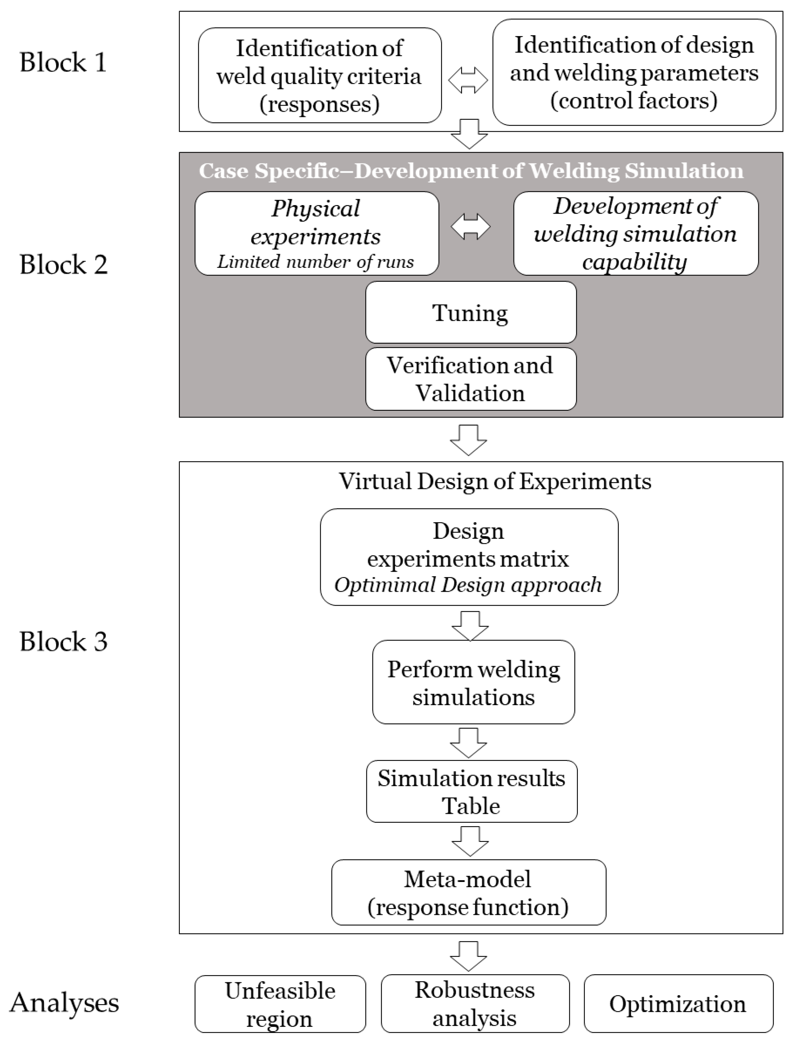
Figure 1. The objective of the virtual design of experiments method is to investigate the effect of the interaction between welding and design parameters on weld quality by combining specific DOE techniques with welding simulation. The method was divided into three main blocks containing a number of steps that will lead to three types of analyses.
The first block is the identification of design and welding process parameters (considered as control factors) together with the identification of weld quality criteria (responses). After the first block, the method was divided into Blocks 2 and 3, named as “Case Specific—Development of Welding Simulation” and “Virtual Design of Experiments”, respectively. Block 2 focuses on preparing welding simulation to the specifics of the case study under consideration.
To date, welding simulations are validated and employed in industrial applications to study macro-level product deformation (distortion) and residual stresses. However, the simulation of other aspects of weld quality such as weld bead geometry, microstructure, and formation of metallurgical discontinuities such as cracks and pores are at a research stage [
29,
30,
31,
32,
33]. Additional aspects of welding simulation that are under investigation are the effects of welding set-up parameters such as gun-to-workpiece distance and beam incident angle [
34,
35].
Thus, Block 2 of the method (see
Figure 1) aims at evaluating whether the current case lies inside the welding simulation validation zone. In the event that the application under consideration is outside the validation zone and the welding simulation is not mature, there is a need for input from physical experiments.
Therefore, prior to jumping into the design of the simulation experiment matrix, a number of physical experiments are required in order to understand the case-based welding phenomenon.
The physical experiments’ results will serve to develop the simulation by tuning the simulation parameters. These physical experiments will also serve to validate the developed simulation model as well as to find reasonable values for the input parameters to the DOE. In an industrial context, physical experiments are usually limited as a result of cost and time. Thus, the ultimate aim would be to reduce the number of physical tests and leave the load of experimentation to simulation.
Once the welding simulation capability has been expanded to simulate the study phenomena, the execution phase “Virtual Design of Experiments” starts (see Block 3 in
Figure 1). This is the block in which DOE is applied. First, the matrix of experiments is designed following an optimal design approach [
36], which can integrate design and welding parameters in the same experimental design. Thereafter, the simulation experiments are conducted. The final step in Block 3, after having obtained the simulation results table, is to build a meta-model, understood as a statistical model that is based on virtual experiments. This meta-model represents the response function embodying the effect of input design and process parameters on the system output responses. From this meta-model, actions can be performed such as optimization, robustness analysis, and definition of unfeasible regions.
The proposed virtual design of experiments method presented in
Figure 1 is designed to be valid in an aerospace industrial context. Aerospace products in general, and aircraft engines in particular, are constituted of components with complex and highly integrated geometries. Questions related to the producibility of component geometries that are raised during design phases concern, for example, welding gun accessibility and the ability to weld different thicknesses.
From this context description, a simplified case consisting of test forged plates made of nickel-based super alloy (Inconel 718) welded with laser beam welding (LBW) are considered as a case study to test the proposed method.
Forged nickel-based superalloys are materials commonly employed in the hot section of aircraft engines owing to their high strength at elevated temperatures [
12]. LBW produces welds with a high depth-to-width aspect ratio, small heat affected zones, and reduced distortion as the heat source is a high-energy density beam. Thus, laser has been considered lately as a promising alternative to the conventional arc welding methods in the aerospace industry [
12,
13].
The application of the method steps for this particular case study are detailed in the coming sections.
2.1. Identifying Responses and Control Factors
The first block in
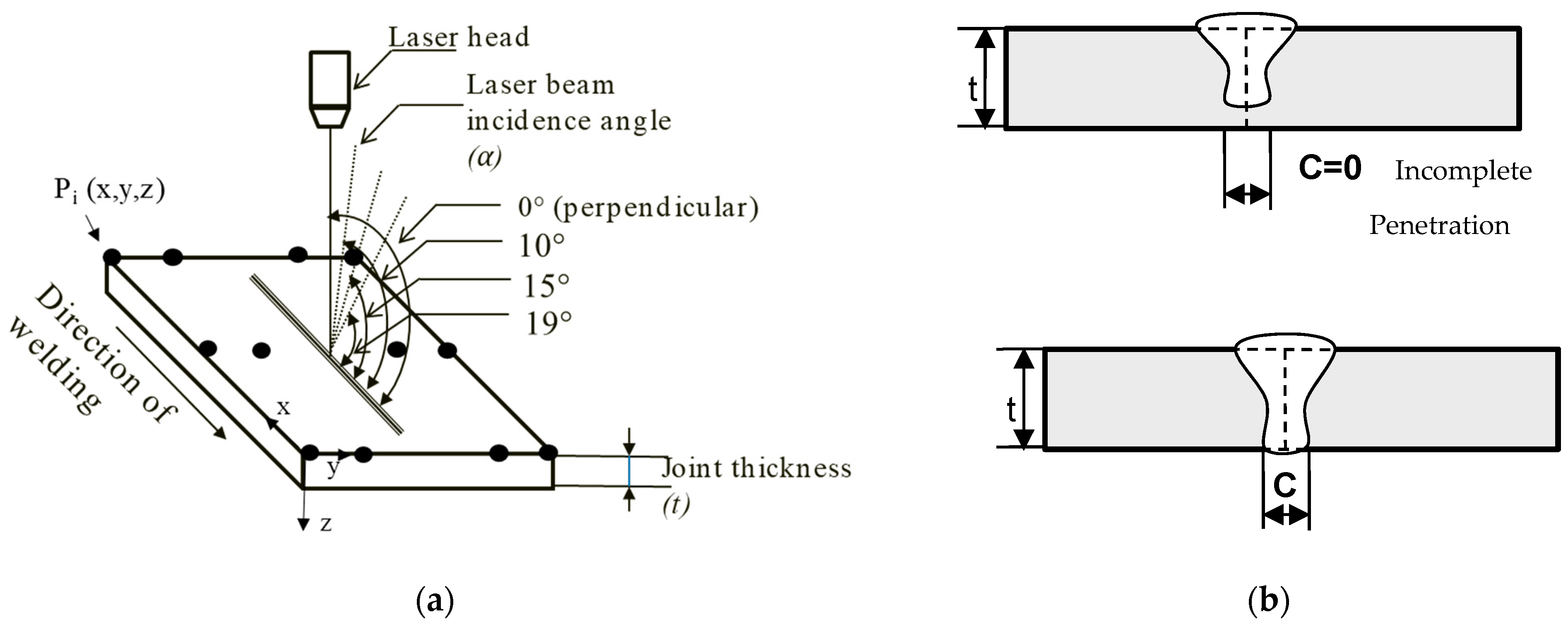
Figure 1 is the identification of the welding responses that wanted to be controlled and the corresponding control factors. The weld quality criteria in this case study is covered by the responses: complete penetration and minimum distortion. Complete penetration is one of the parameters that defines weld bead geometry (see
Figure 2b). Weld bead geometry is an important aspect of weld quality because it can affect product performance [
37]. For example, in aircraft engine components, welds must achieve complete penetration with a minimum bead bottom width to ensure life and safety requirements [
38]. This means that the weld metal must extend through the joint thickness, achieving a minimum bead bottom width; see C in
Figure 2b. Another aspect of weld quality is geometrical distortion, which is a consequence of the built up stresses and shrinkages caused during welding heating and cooling cycles [
37]. Geometrical distortion needs to be controlled within tolerances, otherwise it can cause decrement in product performance [
39] or misalignments in the next assembly level [
40].
The responses’ complete penetration and distortion will be obtained through welding simulation. Welding simulation using finite element analysis (FEA) calculates temperature, distortion, and stress for the geometry under consideration [
41]. Thus, a way to calculate complete penetration is by employing the temperature field and measuring the width of the fusion area at the bottom of the joint (see weld bead dimension
C in
Figure 2b). Distortion will be measured in Z directions for 12 different points, indicated as dots in
Figure 2a.
Two conventional welding parameters considered to have an effect on the complete penetration and distortion, and that can be found in laser welding articles and welding handbooks [
23,
42], are welding speed and welding power. An ideal approach is to weld with a laser beam angle perpendicular to the joint and to consider the same joint thickness in order to have a more efficient and homogeneous heat transfer. However, in this aerospace context, different component geometries incorporating different thickness values will give different accessibilities to the weld, and thus will require welding with different beam angles.
The material type and composition are also critical factors affecting the welding process parameters and thus the response penetration. Each material has different properties such as thermal conductivity that will affect the nature of heat transfer [
37]. In this study, the material is fixed to Inconel 718. However, the reasoning throughout the case study can be applied for any giving material.
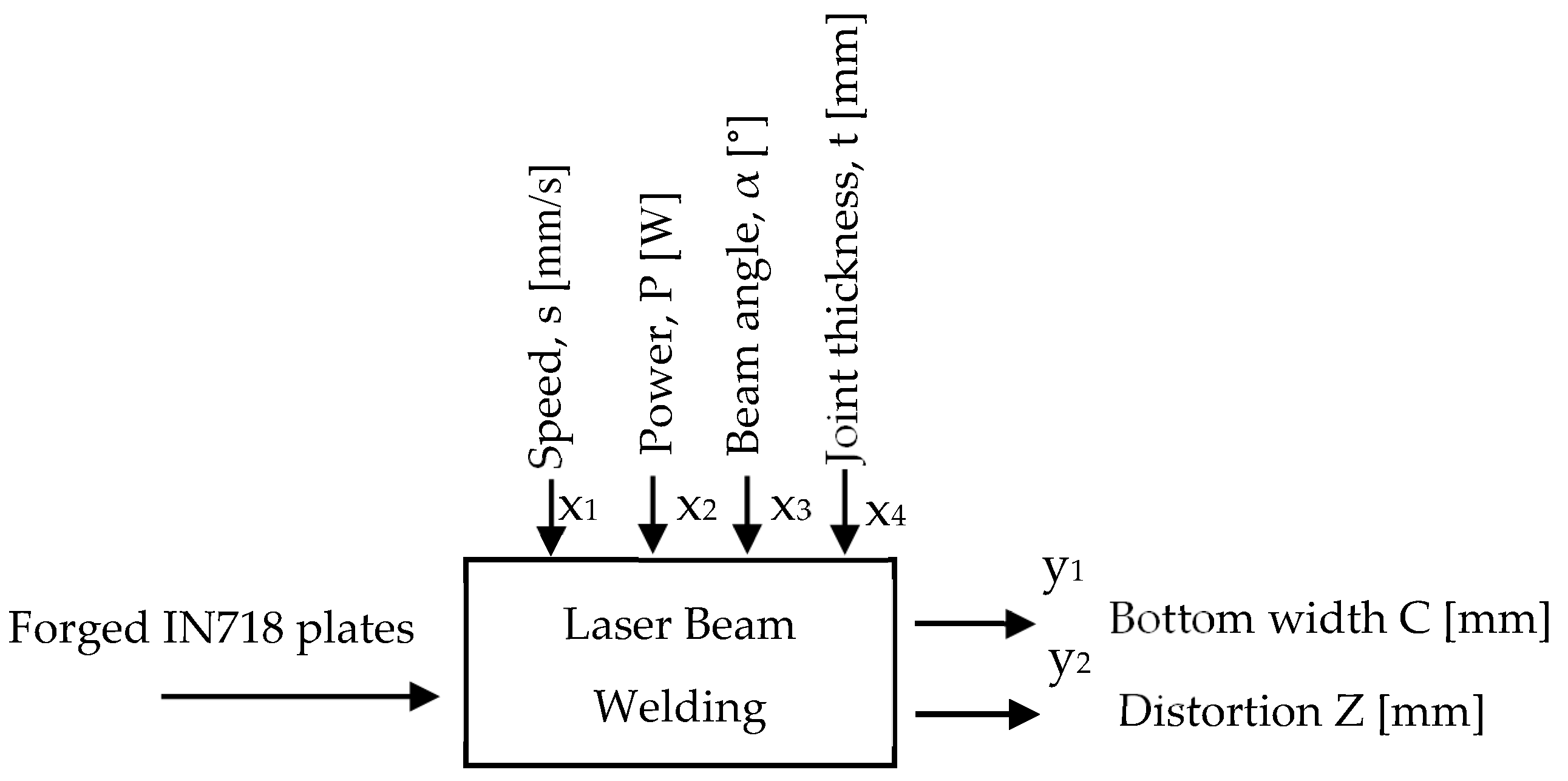
Hence, the control factors affecting the responses’ complete penetration and distortion were identified as laser beam power (P), welding speed (s), laser beam incident angle (α), and joint/plate thickness (t). The last two parameters are derived from the component variant geometries. Other welding process parameters such as shielding gas flow rate and focus are kept constant.
A representation of input and output parameters to the welding process and their units is shown in
Figure 3. To study the effect of the input parameters on the responses, plates of forged Inconel 718 (IN718) with dimensions of 40 × 300 mm and different thicknesses will be laser welded, varying the parameters’ speed, power, and beam incident angle, as shown in
Figure 2a.
2.2. Case Specific—Conducting Physical Experiments to develop Welding Simulation
The effect of tilting the laser beam and how to represent this in the simulation needs to be studied.
Therefore, the purpose of the first step within the block “Case Specific—Development of Welding Simulation” (see
Figure 1) is to perform physical welding experiments with different beam angles.
The objective when developing the welding simulation is to get the correct heat input. Thus, the gap identified concerns modelling the effect that tilting the beam angle has on the heat input. In order to model this effect, there is a need to understand how the weld bead geometry changes according to different beam angles. The physical experiments were conducted for this purpose.
The materials employed for the physical experiments were two plates of forged IN718 with 10 × 40 × 300 mm dimensions. To cut down on the cost of the experiment, two bead-on-plate welds (BOP-welds) were performed in each plate. A BOP-weld is a weld run performed on the top surface of a plate [
37]. The objective of the physical experiments was to observe the varying weld bead shapes depending on the beam angles. Thus, several BOP welds could be performed in the same plate.
The first weld was performed with a laser beam perpendicular to the plate surface (α = 0°). The common practice in industry is to weld perpendicular, or close to perpendicular, so that less energy is dissipated from the laser rays reflection. The welding parameter values for power (P) and speed (s) were realistic values employed to achieve complete penetration according to aerospace standards [
P = 4000 W;
s = 140 mm/min]. The second, third, and fourth welds were run with laser beam incident angles (
α) of 10°, 15°, and 19°, respectively, as shown in
Figure 2a. The values of the welding speed and power were the same as those employed in the first weld.
BOP-welds were preferred in this study in order to remove any error or noise coming from the misalignment of the joint. The welding parameter values for speed and power were kept constant in the four welds to remove the effect of these parameters. A plate thickness of 10 mm was chosen to be thick enough in order to force incomplete joint penetration and observe this phenomenon in at least one of the weld cases.
In addition to these four BOP-welds, historical data on welds with different joint thickness (3, 6, and 8 mm) were gathered in order to support the next step, welding simulation development.
2.3. Case Specific—Developing Welding Simulation
Once physical welds have been performed, the results will serve as input to develop the welding simulation, which is the second step of Block 2 in the method (See
Figure 1). Welding simulation is not an easy task because welding is a complex multi-physical process involving many phenomena such as heating, liquefaction, solidification, and vaporization. Thus, weld pool dynamics; heat transfer; micro-structure dynamics; and structural mechanics including stress, strain, and deformation need to be considered. In order to simulate the welding process in an industrial setting, it is typically necessary to focus on the phenomena that are most important for the scope of the analysis [
43,
44].
In this case, the scope is to model the effect of tilting the beam angle and to achieve the correct heat input to calculate penetration (through temperature distribution) and distortion (deformation).
A standard industrial welding simulation for analysing temperature distribution, deformation, plastic strain, and stress is a thermomechanical problem, which is typically solved using the finite element method (FEM). In this study, FEM will be employed instead of analysing the dynamics of the melt pool, which would require computational fluid dynamics (CFD) using finite difference or finite volume methods. The reason for using FEM is that combining FEM and CFD is a complex problem requiring a very long simulation time, and is thus often infeasible for some industrial designs. The FEM simulation consists of three steps: first, modelling of the heat transfer; second, obtaining the transient temperature field; and third, determining the micro-structure dynamics and structural response [
41,
43].
To start with, some idealization needs to be made to model the heat source for taking into account the effect of tilting the beam angle. There are a number of standard heat source models including the Gaussian surface flux model proposed by Pavelic [
45], the double ellipsoid model proposed by Goldak et al. [
41], and the Gaussian cone heat source model [
43]. The welding technology considered in this case study is laser beam welding, which produces weld beads with a “nail head” shape, as seen in
Figure 2b. Therefore, a combination of a Gaussian surface heat source and a cone heat source that accounts for the digging and stirring effect of the weld is considered as a potential solution to model this case [
42].
Because of this idealization of the heat source, the parameters of the heat model need to be tuned with input from physical experiments. According to Goldak et al. [
41], the most stringent test of the heat model is its ability to predict the fusion zone and peak temperature. Thus, the output expected from the physical experiments is the change on the weld bead geometries for different laser beam angles.
In this work, the aim is to develop the welding simulation capability to cover the effect of the beam angle. Nevertheless, the goal is not to give a physical account or model for the phenomenon, but rather to give an approach on how to employ welding simulation as a design tool to provide directions to designers and manufacturing engineers. A more detailed explanation of the development of the welding simulation and the proposed heat source model is given by the authors of [
46].
The potential parameters selected to define the combined heat source model are the following:
Efficiency: how much energy gets into the material in comparison with the exiting weld gun energy.
Percentage of energy in combined heat source: from the total energy, percentage of energy coming from the Gaussian heat source respective to the cone heat source.
Depth of cone.
Placement of the cone.
Radius of the Gaussian heat source.
Radius of the cone heat source.
The first step is to find the parameters of the heat model by fitting the model to the physical experiment for an angle of 0°. Here, a steady state simulation of the heat transfer is employed. One assumption made is that the temperature distribution surrounding the weld gun is constant after a certain time duration once the weld starts. This enables the temperature distribution, and hence an approximation of the cross section geometry of the fusion zone, in one simulation step.
The next step consists of incorporating hypotheses based on physical considerations on how the heat source would change as a function of beam angle. These are as follows:
The radii of the Gaussian and Cone heat sources would change when tilting the beam angle. This phenomenon would also happen when tilting, for example, a light beam and looking at the projection on a straight surface. For an angle of 0°, it is a circle, while for larger angles, it is an ellipse.
The percentage of fusion area with respect to keyhole area changes with the parameter beam angle. The hypothesis is that when tilting the beam angle, less key hole is created and more conduction occurs. This hypothesis relates to the parameter “percentage of energy in combined heat source”. The more tilted the beam angle is, the more percentage goes to the cone heat source, which models the keyhole.
The decrement of efficiency is based on the growth of the fusion area as the beam angle increases.
Using these considerations as the starting point, the heat model parameters would be tuned based on the results obtained from the physical experiments with different tilted angles (see step 3 in Block 2,
Figure 1). Once the welding simulation is validated and ready, it will be employed to perform the runs or virtual experiments designed by employing design of experiments techniques, as indicated by the steps in Block 3, see
Figure 1.
2.4. Virtual Design of Experiments—Designing the Experiment Matrix
As described by Montgomery [
47], design of experiments (DOE) is a statistical approach that allows for the determination of individual and interactive effects of various factors that can influence the output-responses. The idea is to maximize information with a minimum number of experiments. Thus, in DOE, extreme values (the so-called factor levels −1 and +1) are selected for each variable to create the matrix of experiments. Once the experimental data were obtained, modelling techniques are applied with the objective of optimizing and analysing the robustness of the process.
Within DOE, response surface methodology (RSM) is a collection of mathematical and statistical techniques useful for modelling and optimization [
48,
49]. A standard RMS method used for the design matrix formation is the classical central composite design (CCD) method [
48,
49]. However, the problem of this case study design is that certain factor-level combinations are known in advance to be infeasible. For low thicknesses, combinations of low speed and high power values are undesirable and for high thicknesses, combinations of high speed and low power values are also undesirable, as these combination do not achieve complete penetration. The experimental regions are neither a perfect cube nor a sphere. The input values (or factor levels) of three of the factors considered cannot be varied independently. This condition makes the application of the standard CCD method unfeasible, because this method assumes that all the factors can be varied independently. Thus, with CCD, there will be factor combinations that are nonviable to perform.
Therefore, to solve this problem, the optimal design approach [
36,
50] was proposed as a part of the virtual design of experiment method in order to find an experimental design that satisfies all constraints on the factor values (see step 1 of Block 3 in
Figure 1). More specifically, the custom design platform provided by the statistical data analysis software JMP
® [
51] was selected in this study. This platform allows specifying specific linear constraints between the factors, or input parameters. In this way, optimal designs are custom built for specific experimental settings by an algorithmic approach.
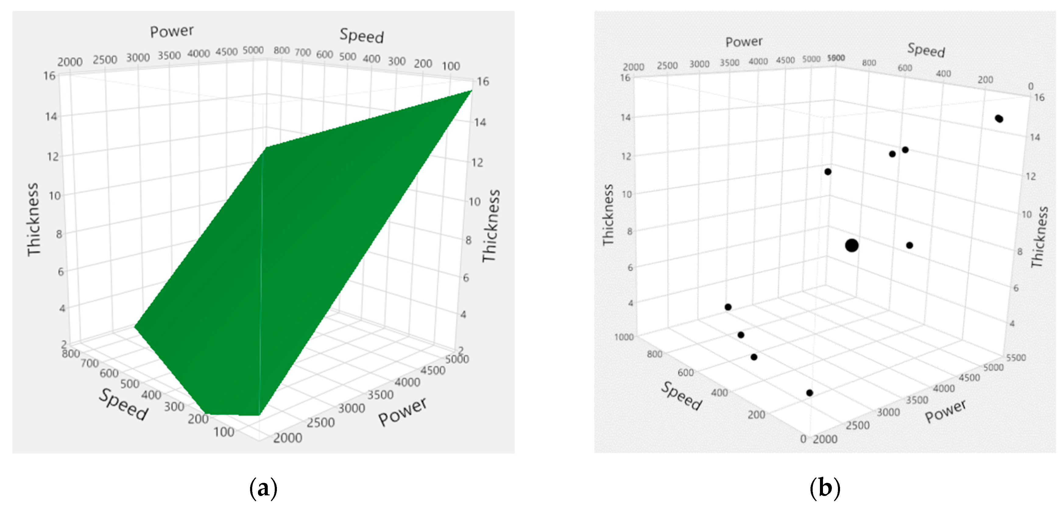
By specifying linear constraints in the custom design platform, it is possible to determine the boundaries of the experimental region, that is, the region of all factor-level combinations that are feasible. Therefore, in order to specify the linear constraint between the three input parameters (power, speed, and thickness), a regression model was built using historical data from previous welding tests. Six different combinations of thickness, power, and speed values were used to build the model. The regression model obtained is expressed in Equation (1) and represented in
Figure 4a. The model has a coefficient of determination of
R2 = 0.7, that is, adequate accuracy. The plane shown in
Figure 4a represents the linear constraint between speed, power, and thickness, which illustrates the experimental region. It can be observed that when thickness increases, power increases and speed decreases.
The regression model expression connected to the plane shown in
Figure 4 is as follows:
Once the experimental region has been defined, the factor levels for each of the four input parameters need to be determined. See
Table 1. Factor levels are defined by extreme values (+1 and −1 as coded values) representing the range of value over which these parameters (or factors) will be varied. In this study, the thickness and beam angle factor levels were the first to be determined. Thicknesses from 3 mm up to 15 mm are commonly employed in the geometry of aerospace components. The range of the parameter laser beam incident angel was determined from accessibility evaluations. The levels for power and welding speed represent typical values employed to weld the preselected thickness range. All values presented in
Table 1 were corroborated with welding engineers.
The input parameter values or factor levels shown in
Table 1 together with the linear constraint expressed in Equation (1) were added to the custom design platform at JMP. The resulting design matrix is shown in
Table 2 and contains 16 runs, that is, experiments.
Figure 4b shows how the different experiments are spread in the experimental design space according to the linear constraint, which illustrates the design matrix in a 3D model.
2.5. Virtual Design of Experiments—Performing Welding Simulations
The 16 runs (see
Figure 4b and
Table 2), which are the result of applying the optimal design of experiments approach, will be performed with welding simulations (see second step of Block 3 in
Figure 1). BOP-welds will be simulated in computer aided design (CAD) plate models with similar dimensions as the plates employed in the physical experiments. The CAD plates are 40 × 150 mm as width × length dimensions, varying the plate thickness according to the values in
Table 2. Having a plate CAD model of half-length (physical plate length was 300 mm) did not affect the results, because the interest was to compare the weld bead geometries between simulation results and physical welds—instead, it saved computational time.
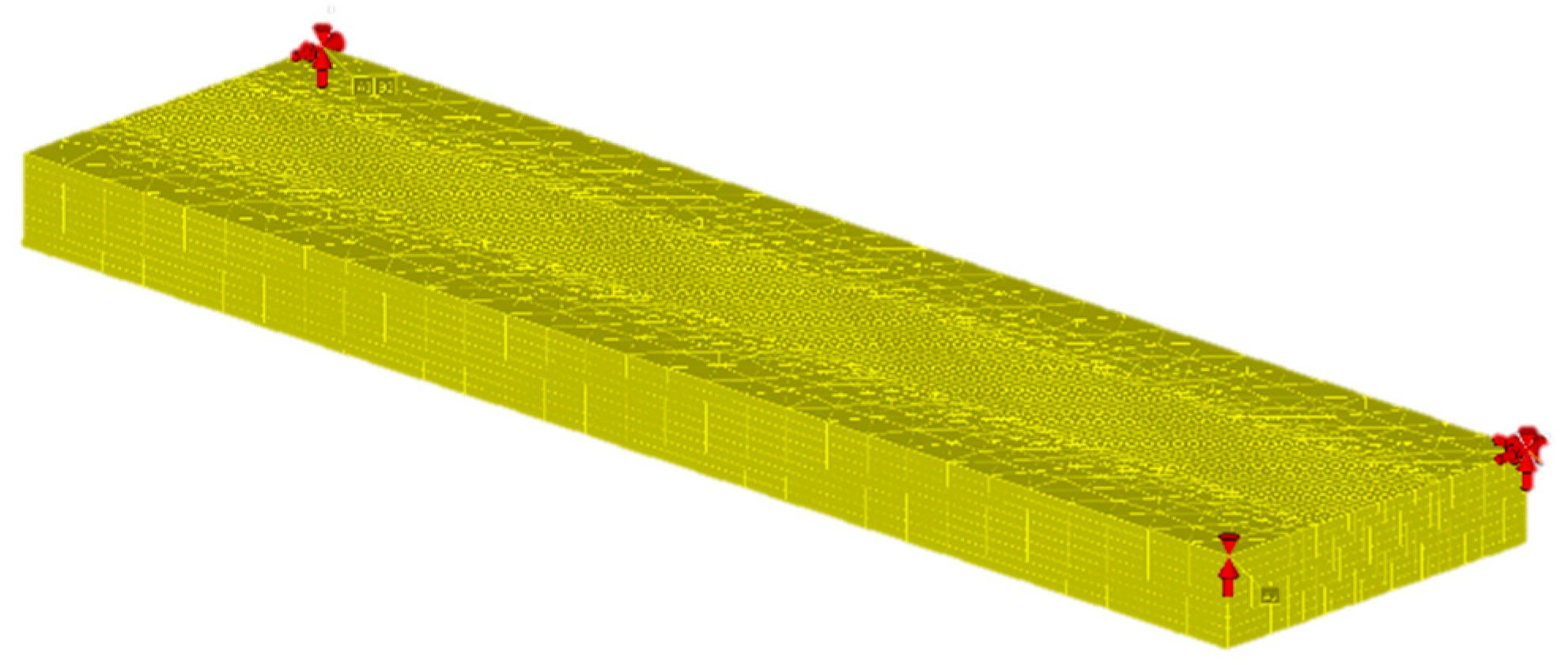
The CAD models were created using an FE software and variation simulation RD&T
® [
52]. In
Figure 5, an example of a 9 mm plate model and its corresponding mesh is shown. The element size around the weld path is approximately 1 × 1 × 1 mm. For every CAD model, the elements are adjusted for the different thicknesses so that each layer of the mesh has the same dimension. The elements further away from the weld path are larger elements, as no big gradients are expected. The mesh size was validated using a smaller mesh, in which each element was approximately 0.5 times the size of the original mesh. No significant change was observed.
The welding simulation is a transient simulation. First, the temperature history is calculated and then the mechanical response is calculated. In this work, microstructure dynamic has not been considered because it is assumed to have only a minor effect on the result [
43]. Adaptive time stepping is employed with a minimum time step of 0.1 s. This means that during welding, the time step is forced to be 0.1 s, and grows after the weld is finished when temperature gradients are decreasing.
3. Results
The description and analysis of the experimental and virtual results from applying the virtual design of experiment method in the aerospace case are provided in this section. There are three main results: (1) physical welding experiments (see block 2 in
Figure 1); (2) a new combined heat source model to cover the effect of tilting the beam angle (see block 2 in
Figure 1); and (3) the welding simulation results and the subsequent meta-model and analyses (see block 3 in
Figure 1).
3.1. Physical Experiments Results
Physical welding tests were performed as described in
Section 2.2 (see also step 1 of Block 2 in
Figure 1) in order to develop the welding simulation and tune the parameters of the heat source model to cover the effect of tilting the laser beam incident angle. The results from the welding experiments are shown in
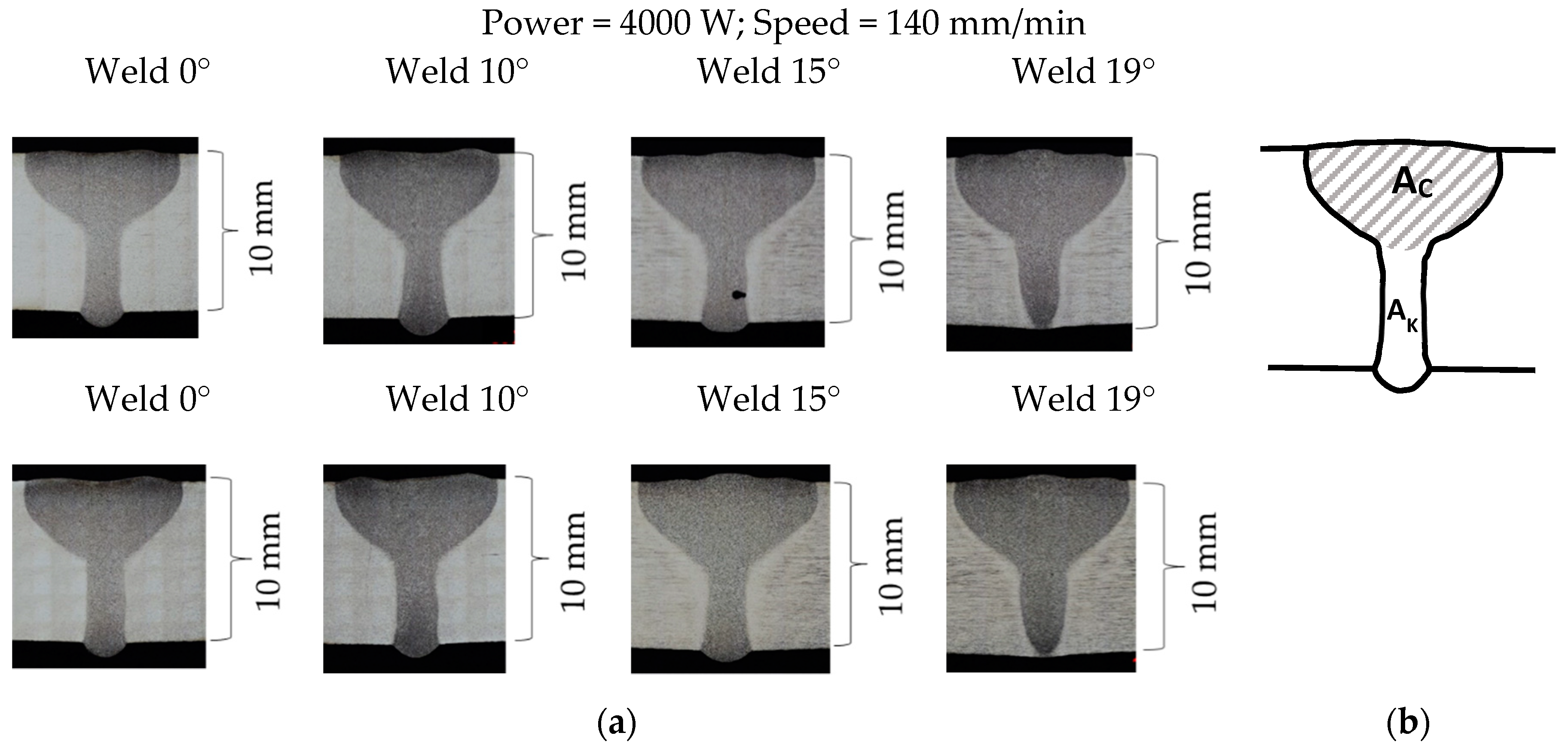
Figure 6. An etch test has been applied to the BOP-welds to reveal the weld bead geometries. This test involved cutting each specimen transverse to the weld axis and applying an etching solution with oxalic acid at 6 V over 20 s, which allowed inspecting the expose surface. This method is adequate for determining the fusion area, thus assessing incomplete penetration. Two transversal cross sections were made for each of the four BOP-welds, which can be seen in
Figure 6a.
Looking at the cross sections in
Figure 6a, it can be observed that the weld bead geometry of this type of laser weld can be divided into two main areas, named in this article as the conduction area (A
C) and keyhole area (A
K); see
Figure 6b.
The conduction area is similar to the weld bead geometry that is obtained when welding is run in conduction mode. The keyhole area represents the actual effect of the keyhole, when material is vaporized and the energy from the laser is directly delivered into the material. These two areas together represent the “nail head” shape typical of laser welds.
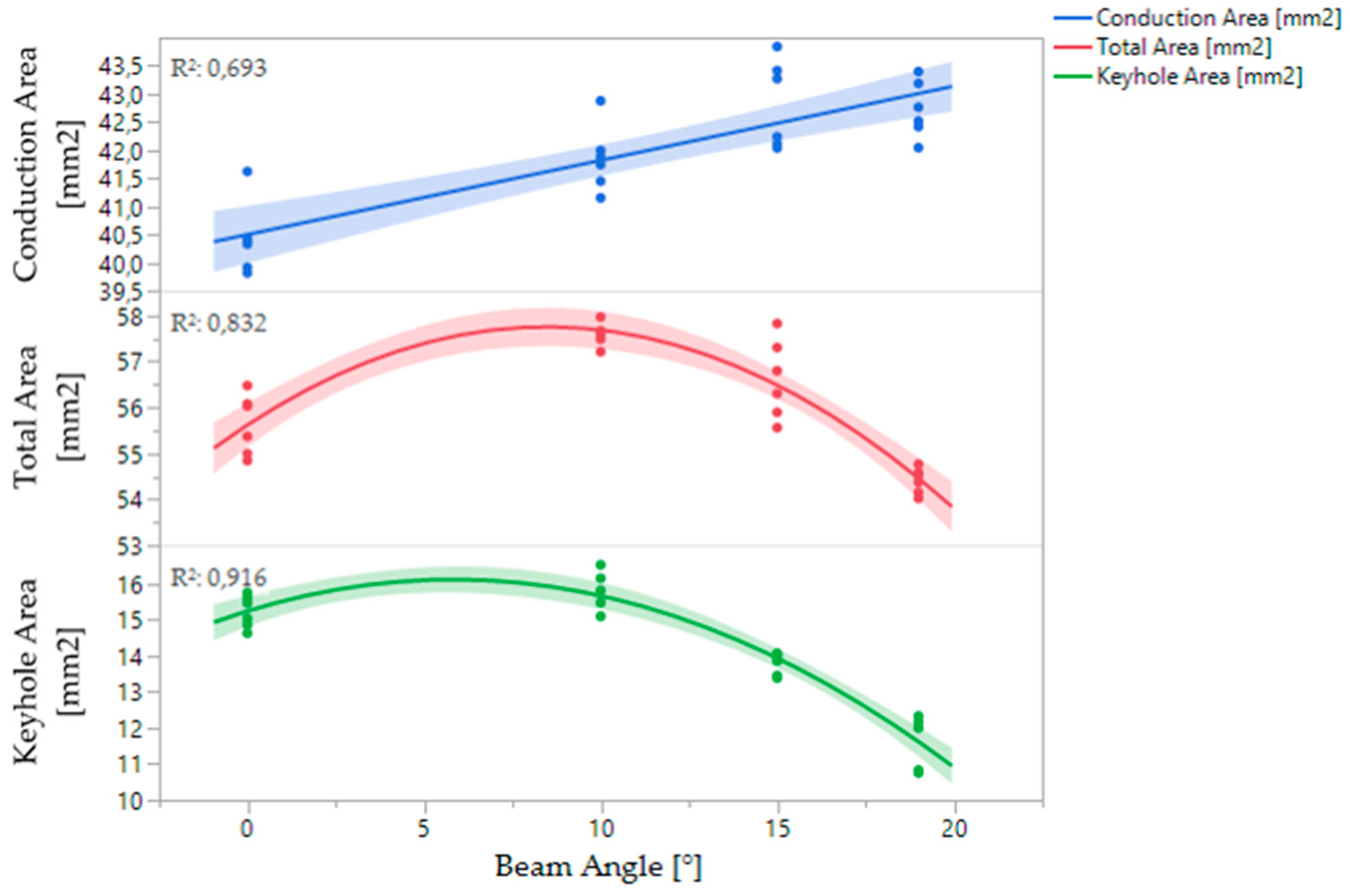
In order to know how these two areas change in relation to the laser beam incident angle, the total, conduction, and keyhole areas of the eight cross sections shown in
Figure 6a were measured three times each. The relation of each of these areas to the beam incident angle is shown in
Figure 7.
In
Figure 7, the graph shows the regression lines and confidence intervals (CI) for the weld bead total areas, as well as the key hole and fusion areas. The values of
R2 indicate good adequacy of the models. Looking at the regression lines, it can be observed that the larger the beam incident angle, the larger the conduction area and the smaller the keyhole area. However, there is a distinction between the effect of the angle on both areas. The conduction area increases linearly from angle 0°, whereas the keyhole area starts to decrease quadratically from angle 5–10°.
3.2. Heat Source Model to Cover the Effect of the Laser Beam Angle
On the basis of the experiment results (see
Figure 6a) and in keeping with the initial hypothesis given in the end of the
Section 2.3, a new combined heat model was proposed (see
Figure 8) to reproduce the fusion zone according to the observed “nail head” shape. The proposed combined heat model is the result of the second step of Block 2 in
Figure 1, called “Developing the welding simulation capability”.
The solution adopted in order to get a reasonable fit of the model was to reverse the cone and employ the placement of this cone as a parameter, as shown in
Figure 8. Above and below the cone, the heat input is set to 0. Additional parameters that also relate to the heat model geometry such as depth of cone, radii of the Gaussian and cone heat sources, as well as the parameters’ efficiency and percentage of energy were been tuned. The weld bead shapes shown in
Figure 6a and the analysis obtained from the graph in
Figure 7 supported the tuning process. An extended description of this process can be found in the work of [
46].
During the tuning process (step 3 of Block 2 in
Figure 1), parameter values for the nominal case (angle 0°) were first obtained. Thereafter, the parameter values for the angle tilted cases were fitted, employing the nominal case values as a starting point. From this tuning process, it can be concluded that the first hypothesis presented in the end of
Section 2.2 with regards to changing the radii parameters values had no significant effect on penetration. Instead, it was found that the parameters that led to major changes on penetration were the placement and depth of the cone, and the efficiency. Therefore, to capture the effect of the beam angle, these parameters were incorporated into the generic heat model (see
Figure 8), and functions relating these parameters with beam incident angle were included in the simulation code.
The same procedure was repeated in order to capture the effect of increasing the thickness. A set of experiments performed with the weld gun perpendicular to the base metal for different thicknesses was employed to fit the parameters. The result showed that by varying the efficiency, the depth, and the placement of the cone, it was possible to reproduce the experimental results in simulation. The dependency of these parameters on plate thickness and tilted angle was modeled by heuristic mathematical models.
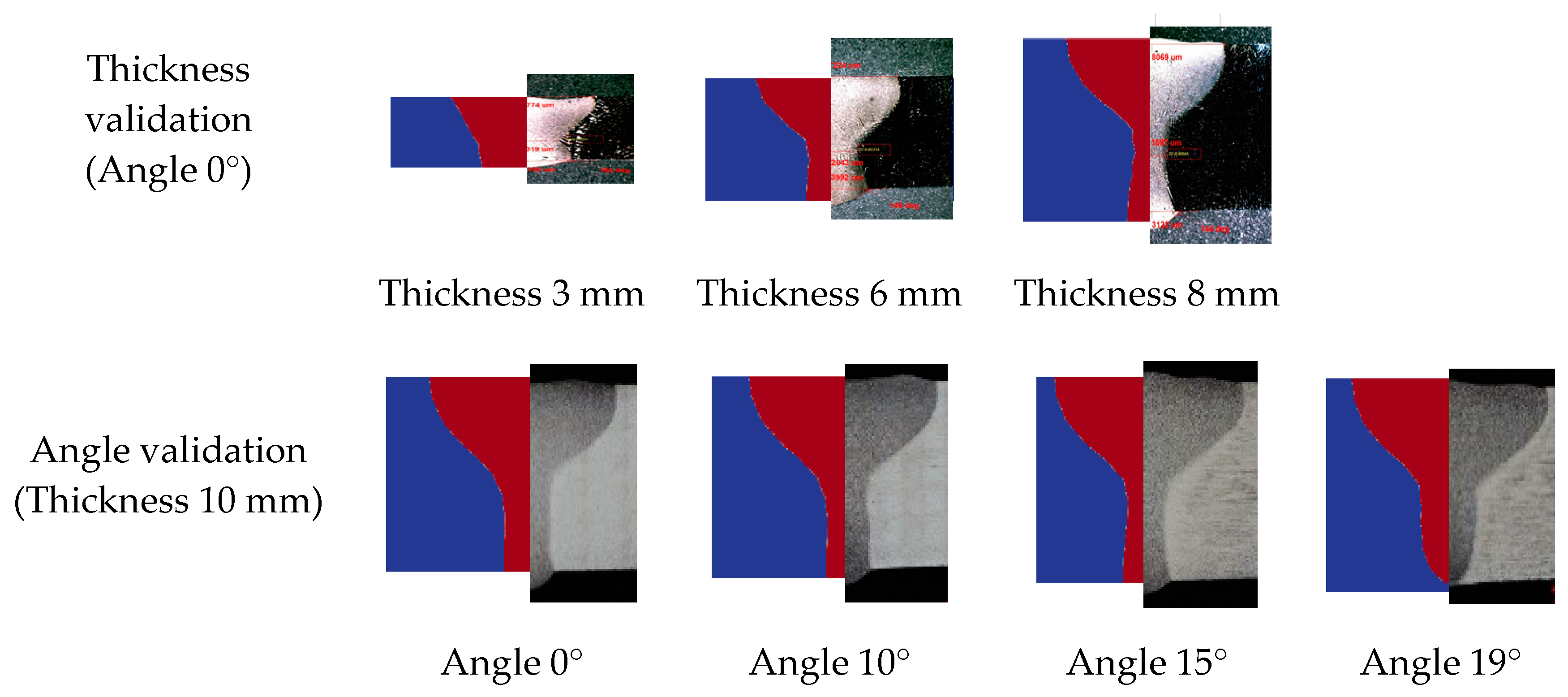
To validate the simulation model (last step of Block 2 in
Figure 1), seven simulations with the same input values as the physical experiments described in the
Section 2.2 were conducted. The results of the validation process can be observed in
Figure 9.
According to Goldak et al. [
41] (p. 122), the most stringent test of a heat model is its ability to predict the fusion zone. Thus, looking at
Figure 9, it can be observed that the simulated fusion zones match the real test fusion zones.
It can be noted that the simulation model proposed was based upon eight experimental results and re-used historical results. However, this is typically the case in industry, in which there is a need to make the best assumption based on the data available. The same applies to the expression of uncertainties and the measurements required to get high fidelity in the virtual results.
3.3. Virtual Experiments Results and Meta-Model
In this section, the statistical analysis and modelling from the virtual experiment’s (welding simulations) results will be presented (see last step of Block 3 and analyses in
Figure 1). The complete table containing all the simulation results can be found in
Appendix A.
The first step of modelling is to determine which are the main factors and interactions that do not have a significant effect on the responses, and removing them from the model.
Using the statistical software JMP
® [
51], the response function (meta-model) for the weld bead dimension C was obtained after reducing the models and can be expressed as in Equation (2):
The bottom width response function, C = f (thickness, beam angle, power), is a first order polynomial equation. Thus, no interaction is significant. Significant factors are beam angle, thickness, and power. In this case, the speed is not a significant factor because it is determined by the values of thickness and power according to the constraint expressed in Equation (1), which represents the experimental region.
The analysis of variance of the mathematical model is presented in
Table 3. The values of F ratio and R
2 assess the adequacy of the model, indicating that this model is adequate.
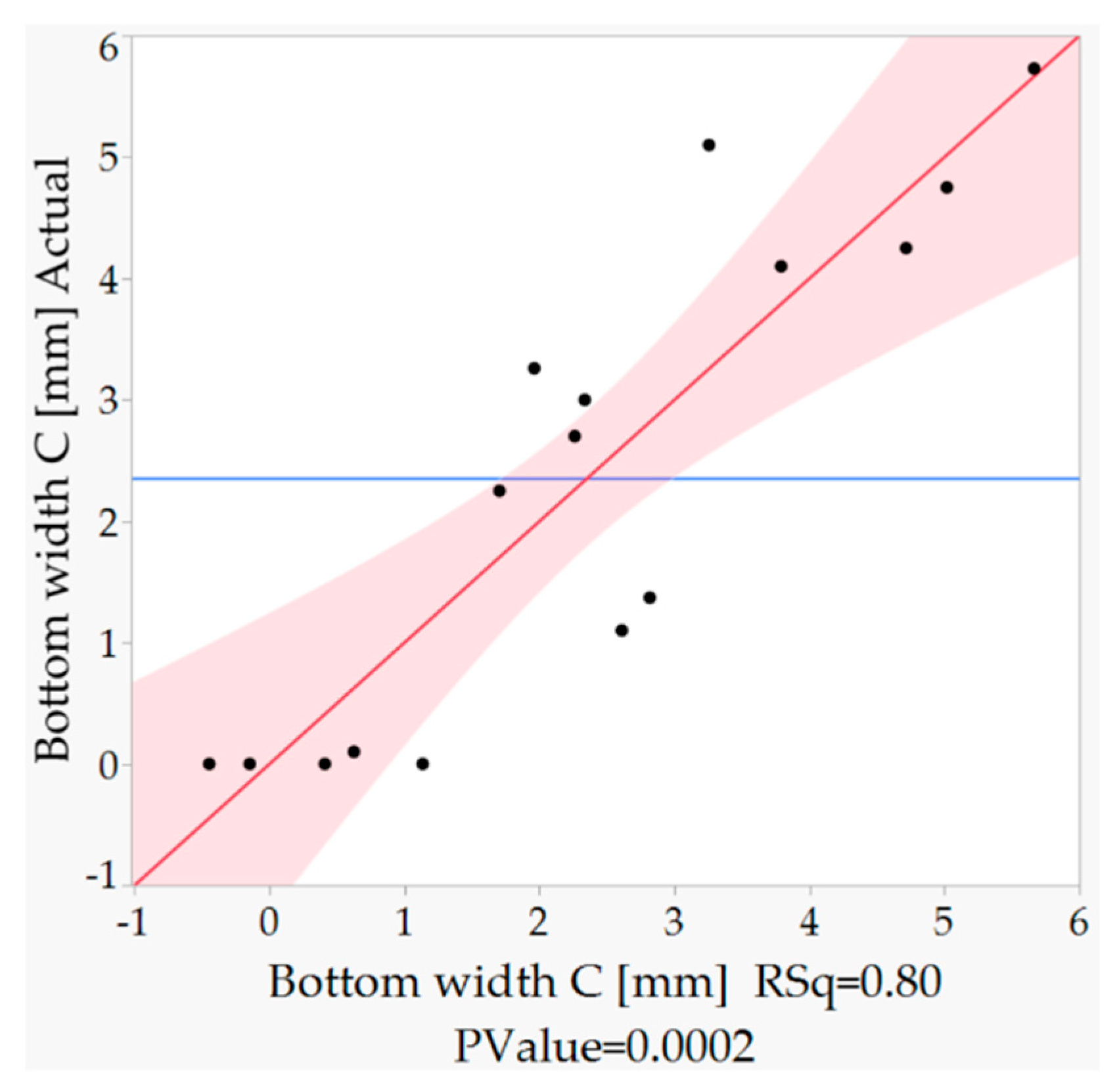
Figure 10 shows the actual versus predicted plot. This plot works as a visual aid to also understand the accuracy of the model by relating observed (actual) values to predicted values. Ideally, the points should be close to the red diagonal line. The red band represents the confidence intervals. The blue line indicates the average. The coefficient of determination
R2 = 0.80 (RSq in graph legend) and p-value = 0.0002 indicate adequate accuracy of the model.
The first analysis that can be derived from the weld bead dimension response function, Equation (2), regards the significance of the beam angle parameter. From the case results and meta-model, designers and process engineers can know that beam angle has an effect on joint penetration (represented by the parameter bead bottom width C).
Therefore, the upcoming questions designers might raise related to thickness and beam angle, which affects component accessibility, are as follows: Which combinations of joint thicknesses and beam angles do not achieve complete penetration? Which values of these parameters give a more stable result? Which are the optimal values? These three questions concern analyses with regards to infeasible regions, robustness, and optimization (see last part of the virtual design of experiment method presented in
Figure 1).
3.3.1. Infeasible Region for Complete Penetration
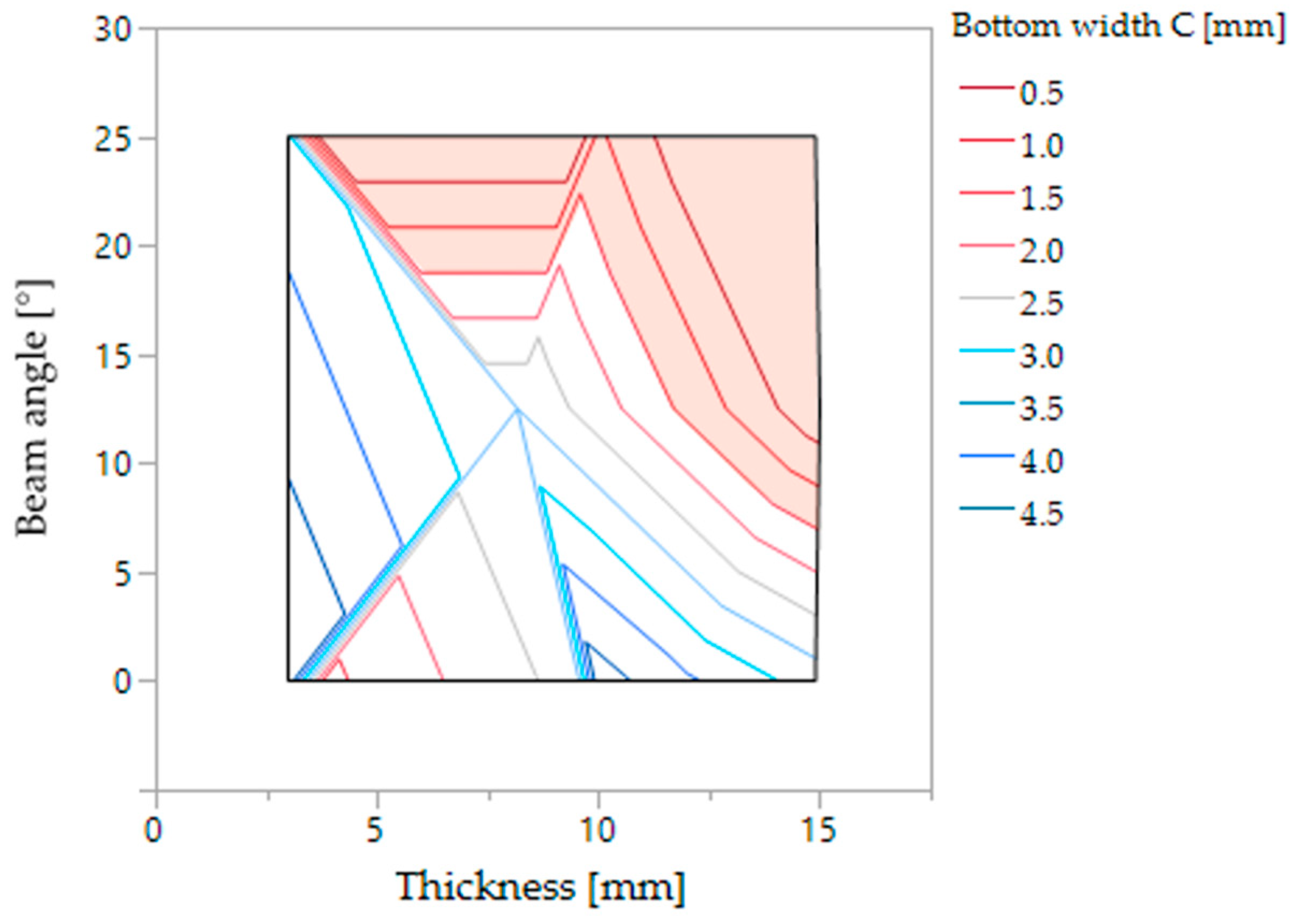
To represent the infeasible region, the graphical technique contour plot was applied. The contour plot in
Figure 11 represents the isolines of the response surface bead bottom width
C on the two-dimensional plane defined by the parameters beam angle and thickness.
C values approximately below 2 mm can be considered unacceptable, that is, requirements on complete penetration are not fulfilled. Thus, all the isolines with values below 2 mm are coloured in red. The rest of the isolines are blue, which represents the combination of thickness and beam angle values that fulfil penetration requirements. On the basis of these requirements, the infeasible region has been marked by colouring it in light red.
For example, thickness values between 12 and 15 mm cannot be welded with angles above approximately 13°. Thus, all aero component geometries containing these thickness values will have accessibility problems, because only low beam angles will be feasible to perform the weld and achieve complete penetration.
3.3.2. Robustness and Optimization of Input Parameters towards Penetration
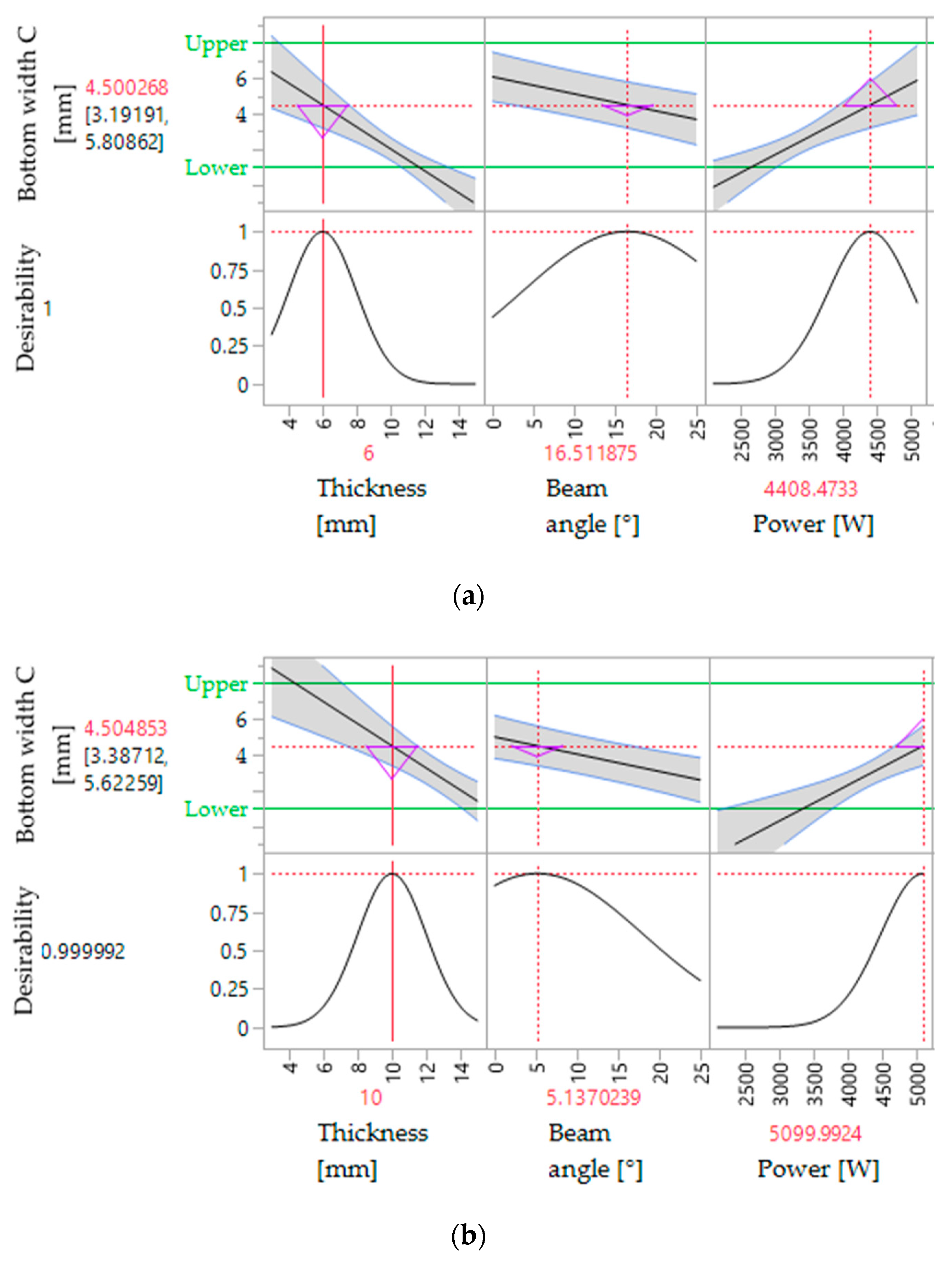
Profiles of the response surface for bottom width
C were employed to analyse robustness and perform optimization, following the gradient descent algorithm implemented in JMP
®.
Figure 12 shows these profiles with black straight lines, which represent cross sections of the response surface for two different thickness values, 6 mm (
Figure 12a) and 10 mm (
Figure 12b). The grey areas around these cross sections represent statistical errors.
To optimize the input parameters beam angle and power for each of the thicknesses, an optimization criterion needs to be defined for the response bottom width C (representing joint penetration).
The straight green lines “Upper” and “Lower” that appear in
Figure 12 represent the upper and lower specification limits set for the dimension bottom width
C. In this example, the objective is to match a target around 4 mm in order to achieve a reasonable penetration.
The optimized values for the input parameters appear in each of the thickness graphs in
Figure 12 in red colour. These values are based on the optimization criterion and the predictive response function already built. For example, if considering a geometry with a thickness of 6 mm (see
Figure 12a), the optimal beam angle and power are 16.51° and 4408 W, respectively. Thus, the bottom width
C optimal value is 4.5 mm, also indicated in red colour.
In addition, a robustness analysis can be performed by examining either the slope of these profile responses or the purple triangles that appear in the graphs. The desirability graphs (graphs located in the second row of each
Figure 12a,b) also give a sense of robustness. Desirability graphs are a piecewise function generated by the statistical software JMP
® that pass through three control points defined by the optimization criterion. Looking at these indicators, it can be observed, for example, that for the 6 mm thickness graph in
Figure 12a and optimal values of power and beam angle, the response C is more robust towards beam angle than towards power. This conclusion could support the designers’ and welding engineers’ decision regarding which parameters can be stricter and which can be more flexible.
3.3.3. Response Surface for Distortion
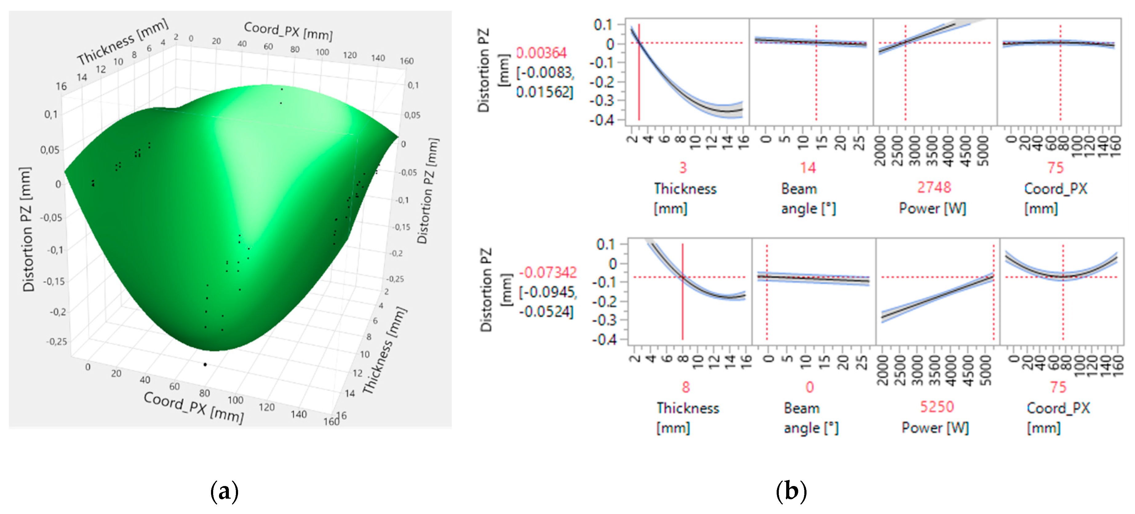
In the same way as for joint penetration, a response surface for distortion in the
Z direction was obtained from the virtual experiment results. In this particular case, the significant individual factors were thickness, beam angle, power, and Coord_PX (representing the position along the
X axis of the points selected to measure distortion).
Figure 13a shows the 3D representation of the response surface for a constant beam angle and power. The dots represent the actual virtual experiment results. From this figure, it can be observed that there are two different distortion modes depending on the thickness values.
This conclusion can serve designers and welding engineers in knowing that for low thickness values, the distortion in the middle of the plate (Coord_PX = 0.75 mm) is positive and for high thickness values, it is negative.
A key finding was that the standard model assumption of quadratic terms for response surface did not capture all distortion modes. Thus, a screening in JMP [
51] of higher order needed to be performed. This screening revealed that the interactions between quadratic terms and individual factors are significant. By adding these terms to the model, it was possible to capture the two distortion modes, as shown in
Figure 13a.
The graphs in
Figure 13b show sections of the response surface (profiles) for 3 mm and 8 mm thicknesses. In the 3 mm thickness graph, it is possible to find values of beam angle and power that can compensate the distortion along the
X axis almost to zero. However, for higher thickness values, as shown in the graph for 8 mm, it is not possible to compensate the distortion, but it is possible to minimize it.
4. Discussion
The results of this article can be discussed in regards to two findings. The first finding involves the results of the aerospace case investigation, that is, the results from the physical welding tests, creation of a new heat source model, simulation results, and subsequent statistical modelling and analysis. The second finding involves the proposed virtual design of experiments method.
4.1. Discussion of the Results
A simplified case was employed to investigate the main and interaction effects of a number of design and welding parameters that are relevant within an aerospace welding context.
Physical welding tests, more precisely, four bead-on-plate welds (BOP), were performed to understand the effect of tilting the laser beam with different angles into the weld bead geometry. The objective was to cover this phenomenon with the welding simulation. An angle of 5° was known in advance to give an acceptable and similar behavior as an angle of 0° from welding expert knowledge. Thus, the interest was to test angles over 10°. Limited resources and high costs permitted the making of only four BOP-welds. In addition, the experimental set-up, because of safety reasons, only allowed programming of the robot to weld at a maximum angle of 19°. These conditions represent limitations when developing the welding simulation.
At the same time, the robot safety limitation leads to virtual experiments and simulation as the way to move forward in order to understand the capability of the welding technology and to be able to explore angles above 19°. The downside is that simulation does not represent a complete answer to reality. Nevertheless, there is the potential to gain more fidelity in the simulation model by, for example, incorporating fluid dynamics into the weld pool.
Besides the absolute values of virtual experiments’ results, the main finding in this study is how these results served to demonstrate that a statistical model can be built with welding simulation to understand the effect of the interaction between design and welding parameters. With this meta-model at hand, infeasible regions for welding producibility can be found and an optimization and robustness analysis can be performed during the design phases.
4.2. Discussion of the Method
The virtual design of experiments method was proposed to model the effect of design and welding parameter combinations (see
Figure 1). In the method, DOE techniques are combined with welding simulation.
The DOE technique optimal design was selected instead of the classical central composite design (CCD), as the experimental region is constrained. Certain combinations of design and welding parameters are known in advance to be unfeasible. This is a common case in aerospace components that are welded, for which a strong interaction between product geometry and welding process exists. Thus, the incorporation of the thickness parameter into the design matrix together with the rest of factors was possible with optimal design. Otherwise, a CCD would have been needed for each of the thicknesses that required investigation. Suppose that three thicknesses were included in the analysis; thus, three design matrices with 16 runs each would have been needed. Instead, with the proposed approach, the total number of runs decreased by more than 50%, and the thickness factor interactions were taken into consideration.
The optimization technique applied in this article is the gradient descent algorithm. This is the algorithm implemented in the statistical software used (JMP
®). Other studies, such as, for example, the one presented by Prakash et al. [
28], have employed evolutionary optimization algorithms. Unlike deterministic algorithms, evolutionary algorithms allow for optimizing the process from a black box perspective without being sensitive to the objective function and constrains. However, evolutionary algorithms cannot guarantee that the optimum found is the global optimum [
53]. In addition, they require more function evaluation, which can increase the calculation cost.
In the case presented in this research, because the response function is already determined using the response surface methodology, the gradient descent algorithm can be applied. As a result, the global optimum can be found for a low calculation cost. A similar approach was presented by Fraser et al. [
54]. In this study, the exterior penalty method was applied after having applied the response surface method. Nevertheless, future work can compare the performance of evolutionary optimization algorithms to the optimization presented in this article for the same case study.
Moreover, the benefits of combining DOE with welding simulation are multiple. One advantage is that simulation allows for performance of a larger number of runs (or virtual experiments) in a very short time in comparison with physical testing. Modelling welding also gives more extended and detailed information concerning welding phenomena, such as the heat distribution and the relationship with welding process parameters. Thus, more information is gained at a lower cost, as also argued by Goldak et al. [
41]. In addition, with welding simulation, virtual experiment runs are performed with the exact numbers given in the design matrix, thus removing input factors’ variation. Errors in the responses and measurement uncertainties also disappear.
On the other hand, there is the gap between simulation and reality. As discussed earlier, the simulation results in this article do not represent a complete answer to reality. Nevertheless, the aim was to present an engineering method to solve these related problems that appear in this type of industrial context. Still, there is room for improvement, which justifies further research by, for example, incorporating more physics into the simulation model.
Future research can also take into consideration input material variation. Currently, the simulation considers nominal plate dimensions. However, it is possible to add variation to the input parameters and analyse the effect on the responses.
With regards to validation, future work can incorporate additional physical welds of some of the 16 runs defined in the experimental matrix, which were performed with simulation.
5. Conclusions
The key contribution of this article is the proposed virtual design of experiment method presented in
Figure 1. By applying this method in the aero-context case, it was possible to build a statistical meta-model employing welding simulation that has allowed the following:
Discovery of the unfeasible region containing the combination of design and welding process parameters for which it would not be possible to achieve complete penetration.
Creation of a surface response that allows the making of optimization and robustness analysis for the responses’ penetration and distortion.
The virtual design of experiments method proposed in this article combines the benefits of experimental design and DOE with the benefits from simulation.
The incorporation of DOE techniques allows for the modelling of the effects of input factors (design and welding parameters) into responses (weld quality criteria), as well as the study of possible interactions between input factors with a minimum number of experiments. The objective in DOE is to maximize information while minimizing efforts. Applying optimal design as a DOE technique leads to custom-built experimental designs for specific settings and constraints, which allows the adaptation of the experimental design to the specific characteristics of the study problem and not vice versa. With optimal design, experimental regions that are constrained because of dependencies between input factors can be investigated, which is a common scenario when investigating product design–welding systems interactions.
The incorporation of simulation into the method enables the capacity for gaining an understanding of the welding process during the product design phases, thus supporting decision making. Executing experimental design with virtual experiments allows for a larger number of runs and factor combinations than when doing physical testing. Welding simulation can also provide detailed representation of welding phenomena, that is, the heat distribution. Thus, this meta-model approach allows access to more results and information, reducing evaluation time and cost.
In conclusion, the virtual design of experiment method proposed in this article will bring the benefit of performing fast evaluations concerning the welding producibility of a number of design variants during early phases of multidisciplinary design of aerospace components. In this manner, a rapid answer can be provided to the OEM about the design and manufacture feasibility of a component variant.
An additional contribution to the welding simulation field is the application of the combined heat source model to cover the effect of tilting the laser beam incident angle.

 ,
, 


