Article

Uncertainty Evaluation in the Design of Structural Health Monitoring Systems for Damage Detection

1
Department of Mathematics and Statistics, Air Force Institute of Technology, 2950 Hobson Way, Wright-Patterson AFB, OH 45433-7765, USA
2
Department of Mechanical Engineering, University of South Carolina, 300 Main Street A237, Columbia, SC 29208-0001, USA
*
Author to whom correspondence should be addressed.
This paper is an extended version of our paper published in 11th International Workshop on Structural Health Monitoring (IWSHM), Stanford, CA, USA, 12–14 September 2017.
Aerospace 2018, 5(2), 45; https://doi.org/10.3390/aerospace5020045
Submission received: 28 February 2018 / Revised: 13 April 2018 / Accepted: 17 April 2018 / Published: 21 April 2018
(This article belongs to the Special Issue Selected Papers from IWSHM 2017)

Abstract

:
The validation of structural health monitoring (SHM) systems for aircraft is complicated by the extent and number of factors that the SHM system must demonstrate for robust performance. Therefore, a time- and cost-efficient method for examining all of the sensitive factors must be conducted. In this paper, we demonstrate the utility of using the simulation modeling environment to determine the SHM sensitive factors that must be considered for subsequent experiments, in order to enable the SHM validation. We demonstrate this concept by examining the effect of SHM system configuration and flaw characteristics on the response of a signal from a known piezoelectric wafer active sensor (PWAS) in an aluminum plate, using simulation models of a particular hot spot. We derive the signal responses mathematically and through the statistical design of experiments, we determine the significant factors that affect the damage indices that are computed from the signal, using only half the number of runs that are normally required. We determine that the transmitter angle is the largest source of variation for the damage indices that are considered, followed by signal frequency and transmitter distance to the hot spot. These results demonstrate that the use of efficient statistical design and simulation may enable a cost- and time-efficient sequential approach to quantifying sensitive SHM factors and system validation.

1. Introduction

Structural health monitoring (SHM) systems are automated methods for determining the change in the integrity of a mechanical system [1]. For aircraft, SHM systems would ideally comprise of embedded sensors working autonomously to provide an in situ, real-time assessment of the structural health. The current assessment of U.S. Air Force airframes is maintained through the Aircraft Structural Integrity Program (ASIP) [2]. The Aircraft Structural Integrity Program (ASIP) utilizes an inspection process that includes the potential for the use of SHM systems to detect damage, which better aligns with the 2008 Department of Defense (DoD) implemented Condition-Based Maintenance Plus (CBM+) policy, which seeks to decrease the maintenance burden by moving the assessment towards condition-based, rather than schedule-based approaches [3]. The SHM system, though, must be validated as required by ASIP. It is the center of discussion in many communities, since the process for SHM system validation remains a complex barrier for the implementation of such systems for on board damage detection.
The validation of SHM systems is multi-faceted and compounded by the numerous conditions and variables, for which the SHM system must demonstrate reliable performance to specification. These include factors related to the following: (1) the non-destructive evaluation (NDE) method (here, it is the configuration of the SHM system itself, with respect to the sensing method utilized and its associated algorithms and models for assessment); (2) the part geometry, material, and condition; and (3) flaw characteristics, including location and orientation [4], as well as varying environmental and operating conditions.
In order to validate the SHM system for all of these categories of factors, performing tests effectively, reliably, and simultaneously on real structures is seemingly infeasible and impractical, because of time, money, and other physical constraints. Therefore, we advocate that work that serves this purpose must begin in simulation and laboratory environments. Factors that can be accurately and mathematically computed may be studied under varying conditions to determine their effect on the SHM response. Those factors that the SHM response is most sensitive to must be considered in all SHM validation analyses, whereas other factors that are not influential on the SHM response need not be.
Indeed, many researchers have started to examine these factors using various methods, including sensitivity analyses, as well as varying factors and model-assisted approaches, with the goal of validating SHM systems for use in real (aircraft) structures [5,6,7,8,9,10,11,12,13,14,15,16,17,18,19]. However, factors are either still examined individually rather than simultaneously, or many assumptions regarding the SHM system configuration and processing are fixed, so that the results are focused on the end measures—such as the SHM system validation metric, known as the probability of detection. The results from these studies are useful. However, if the design considerations or damage indices used for detection are changed, how does this affect the response? The SHM system is not only subject to the detection modality, but also to the configuration, choice of damage index from signal processing, and the environmental and load constraints. How do we know which parameters of the system design and application—from sensor choice, to the environment, to estimating of the probability of detection—was the sensitive or non-sensitive parameter(s) that could detect the damage robustly across all of the intended applications?
Therefore, we advocate for a sequential, model-assisted approach towards the validation of the SHM systems combined with the efficient statistical designs of the experiments, in order to reduce the burden of the SHM system validation. This is achieved by simultaneously examining a number of parameters while also reserving resources, to more deeply address the sources of variation that are the most influential on the SHM response, in subsequent experiments. In particular, we suggest that sensitivity on the SHM response begins, for example, with the basic design configuration and determination of what parameters, with respect to the design and possible damage indices, are the most sensitive and the most robust for the application. This information can then be used to inform subsequent experiments, which then seek to examine other factors, and finally, testing those factors experienced in the operational environment.
In this paper, we demonstrate the utility of using the simulation modeling environment to determine the SHM sensitive factors that must be considered in subsequent experiments. We demonstrate this concept by first examining the effect of the SHM system configuration and flaw location on the response of a signal from a known piezoelectric wafer active sensor (PWAS) in an aluminum plate. Mathematically, we derive the signal responses and, using statistical design of experiments (DOE), determine the statistically significant factors of the SHM system configuration and flaw locations that affect the features or damage indices that are computed from the signal. The amount of variation in the observed damage index, which is attributable to each factor, is quantified and used to identify the damage index exhibiting the most sensitivity to the system design factors and the factors exhibiting the greatest effect on the SHM system response.
As a secondary aim, we demonstrate that these results are obtainable using half of the required number of experimental runs, by invoking an efficient statistical design, namely, the half-fraction factorial. The comparison of the results between the full and reduced (half-fraction) experiment demonstrate the usefulness of this statistical design. The results from this work will demonstrate a method to examine a (large) number of factors affecting the SHM response simultaneously, using half of the required data runs so as to reduce the experimental burden and build a sequential approach to quantifying the sensitivity of the SHM system to all observable factors, in order to enable a demonstration of the system validation.

2. Materials and Methods

We sought to simultaneously quantify the effect of various factors related to the SHM system configuration and flaw location on the SHM response, and in so doing, those factors important for crack detection. We conducted this portion of the SHM validation in a cost- and time-efficient manner, within the simulation environment. We first described the SHM modeling environment and then the structure of the designed experiment from which the simulation data were analyzed.

2.1. Numerical Modeling of SHM Signals

This work assumed the scenario of hot spot monitoring, in which guided Lamb waves traveling through an aluminum alloy 2024-T3 plate were used to detect damage that stemmed from the growth of butterfly cracks from a rivet hole. In many applications of guided waves that were to detect and predict crack growth, the SHM configurations and flaw locations were fixed. Although the usefulness of guided waves was exemplified [6,7,8,9], the sensitivity of the response (detection) to the configuration was not explored. As a result of part geometry, it was not always possible to replicate the same configuration in real-world use. Therefore, this experiment to determine which aspects of the SHM configuration were most sensitive to the detection, was warranted.
The numerical modeling included the following assumptions about the hot spot monitoring scenario: Firstly, the sensors and transducers that were employed were piezoelectric wafer active sensors (PWAS), whose usefulness for damage detection of rivet holes had been examined [20,21,22,23]. We assumed that the transmission medium was an infinite homogeneous thin plate of aluminum (2024-T3), with a constant thickness of 1.6 mm and a density of 2780 kg/m3. All of the defects were invariant in the z-direction, thus, the rivet hole and damage were uniform from the top of the plate to the bottom of the plate. Emergent cracks were symmetric and appeared on diametrically opposing sides of the rivet hole with equal lengths on both sides. Flaw size was defined as the combined lengths of the cracks from both sides of the hole. Finally, cracks were modeled as infinitely thin, straight notches, with no wave propagation through the crack faces.
The initial SHM configuration is shown in Figure 1. The transmitting sensor would send out a Lamb wave with a particular frequency. When the wave hit the damage location, the damage location acted as a new wave course. The received signal at the receiver (R-PWAS) was comprised of two parts: the direct incident waves from the transmitting sensor (T-PWAS) and the scattered waves from the damage source. We employed the finite element method (FEM) to solve for the scattered waves from the damage source. As shown in Figure 1, R-PWAS was fixed at 15 mm from the rivet hole. The location of the T-PWAS (distance from rivet hole to excitation) was allowed to vary, as was the T-PWAS incidence angle to the damage (θ), in addition to PWAS size. Similarly, although R-PWAS was a fixed distance, the incidence angle to the damage was also allowed to vary (φ), as was the Lamb wave frequency. Finally, we also allowed the flaw size to vary, creating six different factors to examine that were associated with the SHM configuration and flaw size.
In order to capture the resulting signals at each of the combinations of the varying factors (transmitter angle, receiver angle, frequency, sensor size, distance to excitation, and flaw size), we utilized the combined analytical/finite-element approach that was detailed in Shen [21]. Fundamentally, the approach followed the following steps:
  • Built a model of the reduced domain near the rivet hole in ANSYS (ANSYS® Mechanical APDL) with a sensing circle and non-reflecting boundary conditions.
  • Evaluated the time-harmonic solutions to the wave scattering problem for frequencies of 2–1000 kHz at 2 kHz intervals, using the finite elements in ANSYS.
  • Post-process FEM outputs generated complex scatter-cubes with wave-damage interaction coefficients (WDIC),
  • Imported WDIC to Waveform Revealer 2-D (WFR-2D) in order to generate signal data analytically.
The WFR-2D code was produced by the Laboratory for Active Materials and Smart Structures at the University of South Carolina and was designed to produce simulated signals under varying conditions, akin to the experimental configuration that was examined here [24].

Finite Element Modeling

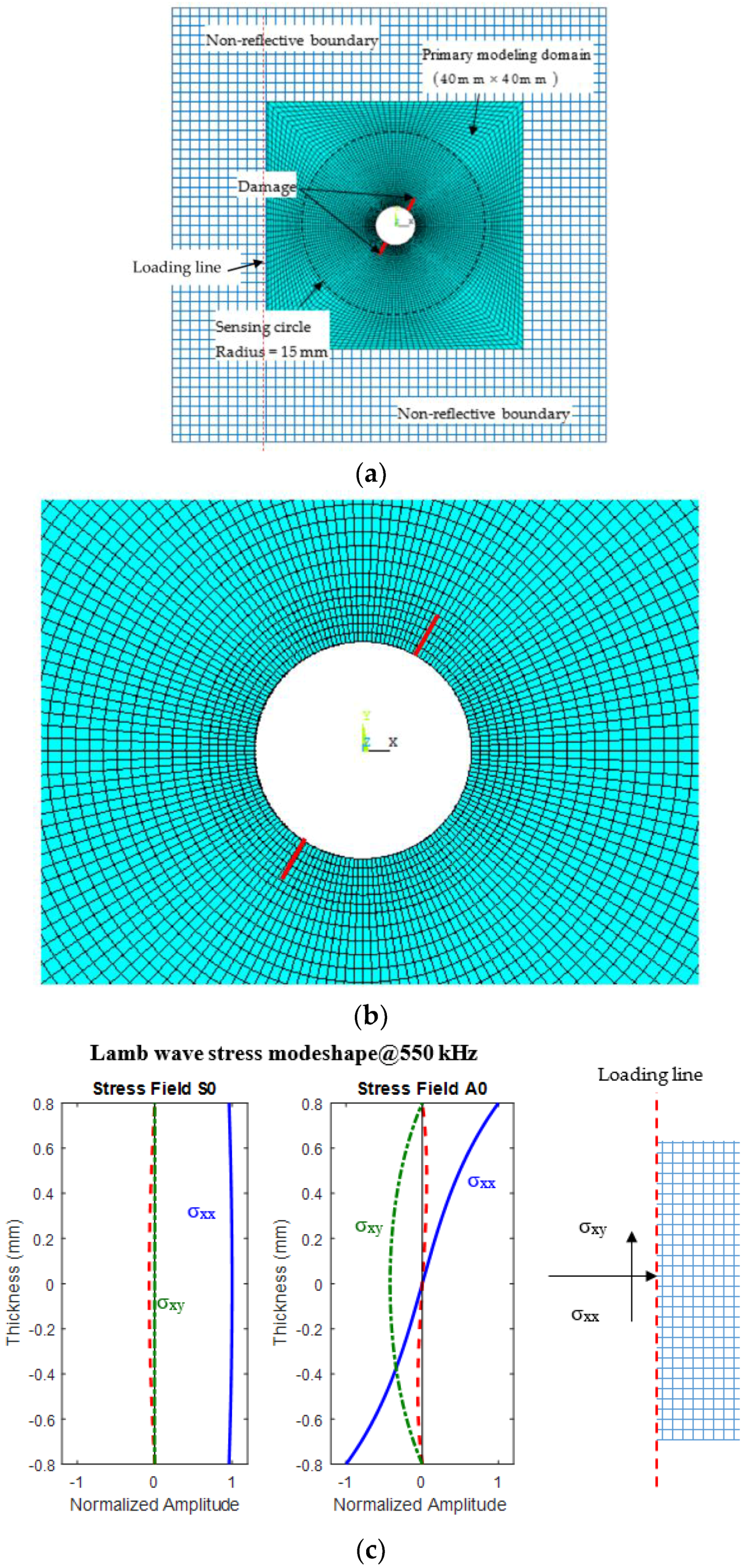
This section briefly describes the FEM environment and related assumptions. A FEM model in ANSYS Mechanical APDL was constructed for each flaw size and transmitter angle pair in order to produce the WDIC required by the WFR-2D. The harmonic analysis was conducted on each model over 500 frequency steps. During the simulation, the domain was independently solved with 183,720 equations at each step. Having assumed a sufficient distance from the transmitter to the modeled region, the incident Lamb wave was represented as a straight-crested wave impinging on the left boundary of the primary computation domain. The non-reflecting boundary conditions, described by Shen and Girugiutiu [25] and used by Bhuiyan, et al. [26], were applied to simulate an infinite domain. The physical dimensions of the model were chosen to be an 80 mm square. This included 20 mm on each side for the non-reflecting boundary, and a 40 mm center square that served as the primary computational domain. The rivet hole was located in the center of the computational domain, and 160 nodes along a sensing circle were identified for collecting model outputs. The distance from the rivet hole to the sensing circle was chosen to be 15 mm to allow sufficient distance for complex modes to evanesce. The computational domain is illustrated in Figure 2. An overall FEM model is illustrated in Figure 2a, the zoomed in view of the damage region is shown in Figure 2b, and the boundary conditions are shown in Figure 2c. There were two nodes disbanded along the crack faces in order to simulate a crack. The detail of the crack modeling was illustrated by the authors of [22]. The boundary conditions were applied along the loading line. The Lamb wave stress mode shapes were converted into nodal forces and then applied at the nodes, in order to generate the desired Lamb wave mode (S0, A0). For each frequency from the FEM solution, the real and imaginary values for the displacements in x and y along the upper and lower nodes of the sensing circle were collected and saved as outputs. When combined, this provided eight output files with 160 × 500 entries each. These displacements were converted into damage coefficients for the WDIC by following the method described by Bhuiyan et al. [22]. Finally, the received signals were generated in WFR-2D after inputting the specific transmitter and receiver angles, transmitter distance, frequency, and flaw and sensor size.

2.2. Experimental Factors and Damage Indices

There were six factors that were varied for this experiment—namely, the transmitter angle, receiver angle, frequency, sensor size, distance to excitation, and flaw size—each at two fixed settings. The levels of each of the factors are provided in Table 1 and were chosen based upon experience and previous results [22]. Comparisons of the combined levels for each factor resulted in a total of 26 = 64 experimental design settings from which to recover signals for both the flaw state and baseline (signals that were the result of a plate with a rivet hole containing no crack). The signal output was measured as the vertical displacement (in nanometers) at the receiver location. An average analysis window size of 40 microseconds was used in order to compute damage indices. We chose to examine three common and simple damage indices, all of which were relative to the baseline signal, namely: a correlation coefficient, the sum of squared deviation, and the difference in peak amplitude. The damage index for the correlation coefficient (DIcc) (ρ) was given as follows:
1 ρ = 1 [ t min t max f ( t ) g ( t ) d t / ( t min t max f 2 ( t ) d t t min t max g 2 ( t ) d t ) ]
where f and g represent the baseline and damage signals within the time window [tmin, tmax]. The Sum of squared deviations (sqdev) compares the baseline (f) and damage (g) signals and is computed for the discretized observed signal values as follows:
t min t max ( g ( t ) f ( t ) ) 2
As the window size was fixed, the sum of squared deviations provided the same information as the mean squared deviation. Finally, the difference in peak amplitude (diffPA) was computed by taking the difference in the maximum amplitudes between the two signals within the analysis window.

2.3. Statistical Experimental Design and Analysis Methods

The six factors were varied, each at two levels generically referred to as “high” and “low”, for a total of 64 experimental runs: one for each combination of high and low levels across all of the six factors. The baseline signal was computed separately for for 25 experimental configurations (all factor levels of Table 1, except for flaw size). Table 2 provides the settings for each of these 64 runs. These settings were specifically chosen so as to utilize an efficient design of the experiments, namely, the 2k factorial design (here k = 6 for six factors and 2 indicated that each factor was assessed at two different levels). One of the efficiencies of this design was in its ability to test the factor level combinations through a reduced number of experiments, namely, half or even one-fourth of the number of experiments. Therefore, the goal of this experiment was twofold. Firstly, we demonstrated the sensitivity for each of the three damage indices to the various SHM design settings, using the full factorial design (26 runs), and secondly, we conducted the analysis on a fractional factorial design using half of the number of runs (26−1) and compared the findings. If the statistical design was efficient, we should have seen comparable results between the full design (26 experimental runs) and the design used that half of the number of runs (26−1 = 32 experimental runs). The factorial design that used half of the number of runs was called the half-fraction factorial design.

2.3.1. Full Factorial Design

The signals for the baseline and each of the experimental runs were generated as previously described and the three damage indices were computed. The statistical analysis was conducted using the analysis of variance (ANOVA) to determine which effects were statistically significant. Any significant interaction effects were examined using Bonferroni-adjusted multiple comparisons, and plotted for interpretation. A significant interaction between two factors would indicate that the effect of the first factor, for example the transmitter angle, on the damage index depended on the level of a second factor, for example the frequency. Since there were six factors in this analysis, there was the potential for all six of the factors to interact, thereby producing a six-way interaction as well as a five-, four-, three-, and two-way interaction between the factors.
To assure that the modeling assumptions that were required by the ANOVA technique were met, each damage index was examined for normality, using the Shapiro–Wilks test [27], and the variance was examined. All three damage indices failed the test for normality. Therefore, each damage index (DIcc, sqdev, and diffPA) was transformed using the natural log (ln) (labelled as lnDIcc, lnsqdev, and lndiffPA, respectively) prior to conducting any analysis. Since there was only one run per experimental setting, conducting a formal statistical analysis was complicated, because we had no duplicate runs with which to estimate (random) error. That is, once the estimating effects for all six main factors—namely, 15 two-way, 20 three-way, 15 four-way, 6 five-way, and 1 six-way interaction(s)—there were no degrees of freedom to estimate error, and therefore, there was no estimate of mean square error to perform statistical testing. Subsequently, in order to estimate the error in the ANOVA, we applied the commonly used sparsity of effects principle [28] and assumed that any five- or six-way interactions were negligible, in order to provide degrees of freedom for error.
Furthermore, we used normal probability plots of the factor effects in order to identify any potentially significant effects and to ensure that any possible higher order interactions (in this case, two- or three-way interactions) would not be missed [29]. The normal probability plot leveraged the modeling assumptions of the ANOVA in order to plot the overall effect of each factor against its expected value under normality. In the ANOVA, the random error was expected to be normally distributed with a mean of zero and a variance of σ2. Therefore, the observed factor effects were assumed to be normally distributed and the specific values that were observed were used to compute a (empirically) cumulative normal probability. This was achieved by ordering the observed values from smallest to largest and estimating the cumulative normal probability for the ith ordered effect as the (i − 0.5)/n quantile of the normal distribution, where n denoted the number of effects. Factors with small effects would lie along a straight line within the plot. Factors with large effects on the response would deviate substantially away from the other plotted factors. The use of the normal probability plot allowed us to use modeling assumptions to not only identify large, potentially significant effects, but to identify those effects that were essentially negligible (near zero effect), in order to use these small effects to estimate error. The use of the word “effect” was both colloquial and statistically specific. A factor’s effect was estimated by a linear combination of the observed responses from all of the experimental runs. In essence, for a particular factor, for example the transmitter angle, we would add the observed responses for all of the runs, where the transmitter angle was set to high, and subtract the observed responses for all of those runs in which the transmitter angle was set to low. This linear combination was then divided by (n2k−1) to get an estimate of the factor’s (average) effect. The standard DOE textbook explains these calculations and how to efficiently compute these effects for all factors and interactions [29].
Therefore, all assumptions of potentially negligible higher order interactions and negligible lower order interactions, and the main effects, were visually confirmed through normal probability plots prior to conducting the ANOVA. Finally, all statistical analyses assumed an inference wise Type I error rate of 0.05.

2.3.2. Half-Fraction Factorial Design

Fractional factorial designs had specific structures that allowed comparable inference while conducting a reduced number of experimental runs [29]. However, in order to reduce the number of runs, aliasing, among the factors, and interactions in the fractional factorial design occurred. Aliasing in statistical designs occurred when several effects (of main factors or factor interactions) were estimated simultaneously and therefore could not be disassociated. In other words, the effects were confounded together. This confounding occurred mathematically as a result of the reduced number of runs. This was because, when using only a fraction of the required number of experimental runs, the linear combination of the high and low levels that were used to compute the factor effects became duplicative for two different factors/interactions when using half of the runs, and duplicative for more than two factors/interactions when using less than half of the runs. That is, these linear combinations were unique when using all of the experimental runs in a full factorial design, but with fewer runs completed, they would produce equivalent estimates for certain factors/interactions in designs of reduced runs. In other words, if you only performed a fraction of the factor level combinations, then you would lose some information about these factors or their interactions. Therefore, when confounded, a significant effect that was found might have been attributable to any of the factors that were aliased together; the model and statistical design were unable to disassociate the factors because of the reduced number of runs that were performed. Depending on which runs were performed, and which were not, the effects that became confounded together were determined. However, there were special fractional factorial designs in which confounding might have been mathematically designed, such that the effects of interest were not aliased with each other, and ideally, only aliased with higher order interactions. Such interactions were deemed negligible to the experimenter. In this manner, if there was a significant effect found, it was likely attributable to the effect of interest and not to the (negligible) higher-order interaction. For instance, say the effect of transmitter angle (A) was confounded with the five-way interaction between receiver angle (B), frequency (C), sensor size (D), distance to excitation, and flaw size. Then, if found statistically significant, we might have concluded that this effect was significant, primarily because of the influence of the transmitter angle and not from the aliased five-way interaction. There were many ways to create the aliasing when reducing the number of experimental runs in a factorial design. The ability of a fractional factorial design to alias the main factors with higher order interactions was classified by design resolution.
For instance, in this analysis we conducted the 26 factorial experiment for a second time using only half of the number of runs, that is, in only 26−1 = 25 number of runs. This design was called a half-fraction factorial design, since we were only using 32 of the 64 required runs to examine every high/low combination of all of the six factors. This meant that there would be confounding, in which two factors/interactions would mathematically produce the same exact effect when calculated from the observed responses. However, by deliberately picking 32 of the 64 experimental configurations to run, we accomplished what is called a resolution VI design, in which the factors of interest to us were estimated separately and not aliased (or confounded) together. A resolution VI design for our experiment meant that each main effect (A through F) was aliased with specific five-way interactions (which we deemed as negligible by the sparsity of effects principle); two-way interactions were aliased with four-way interactions (also likely negligible as a higher order interaction); and three-way interactions were aliased with each other. Therefore, if a main effect, such as transmitter angle (A), was significant, although it was aliased with the five-way interaction—between receiver angle, frequency, sensor size, distance to excitation and flaw size (BCDEF)—we attributed the effect to that of the transmitter angle (A) rather than the complex, five-way interaction (BCDEF). The alias structure for our resolution VI half-fraction factorial design is listed in Table 3. The statistical analysis included the same steps as for the full factorial analysis, although now the normal probability plots and resulting ANOVA were conducted on 32 runs instead of 64. For this portion of the analysis, the goal was to determine whether the main sources of variation in the SHM configuration could be identified with half of the required experimental runs. If this is achievable, this reduced design would result in a significant savings with respect to time and cost in the SHM validation.

3. Results

We divided the results into two subsections in order to describe the factors for which there were significant differences among the damage indices, as determined through the full factorial design and, secondly, to demonstrate the feasibility of using the half-fraction factorial design to determine the significant sources of variation.

3.1. SHM Configuration Factors Producing the Most Variation in the SHM Response (Damage Index)

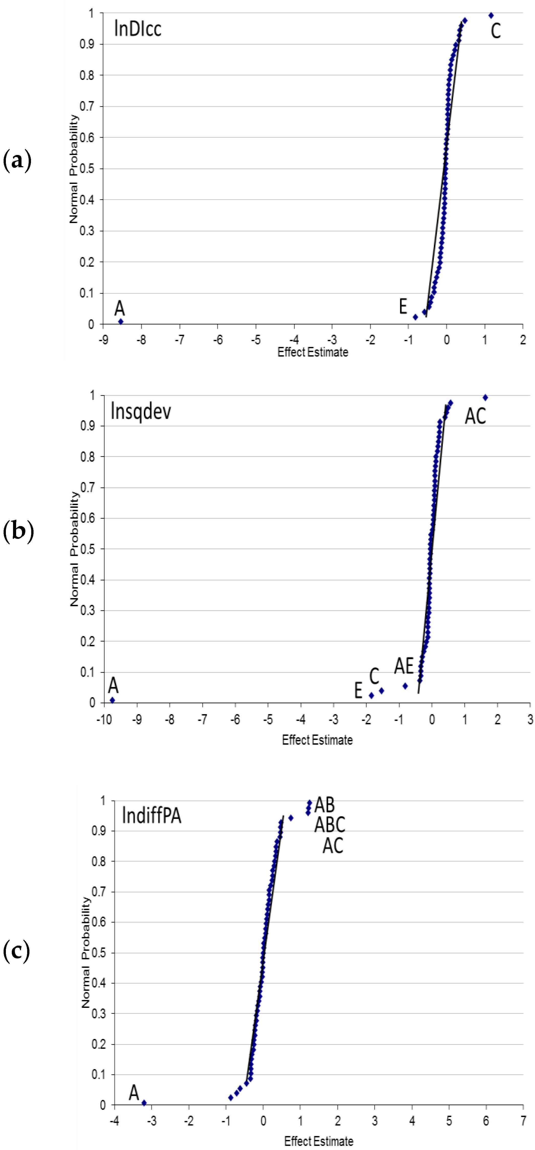
Figure 3 shows the normal probability plots for lnDIcc, lnsqdev, and lndiffPA in the full factorial design of 64 runs. Recall that this plot visually demonstrates the probability that is associated with the observed effect on the response for each of the factors and interactions under the modeling assumptions that are associated with the ANOVA. Those factors that had small/negligible effects hovered around the effect size of zero and fell along a straight line in the normal probability plot. Effects that were labeled in Figure 3 (using labels from Table 1) denoted reasonably large effects and were located farther away from the line. Overall, the factors that had the largest effects varied by the damage index that was chosen for the detection of damage. Across all three of the damage indices, the transmitter angle (A) appeared to have the largest absolute effect (Figure 3). The negative effect that was estimated for transmitter angle in each of the damage indices indicated that the observed damage index was generally higher for the low setting of the transmitter angle than for the high setting. In other words, the observed response for each of the damage indices was larger at a lower transmitter angle. The distance to the excitation (E) also had a reasonably large effect for both lnDIcc and lnsqdev, however, it did not have a large effect on lndiffPA. There were no large interaction effects for lnDIcc, but lnsqdev appeared to be sensitive to the combined levels of the transmitter angle and frequency (interaction AC), as well as the transmitter angle and distance to excitation (interaction AE), both of which are marked in Figure 3. With an effect size value over 1.0, lndiffPA exhibited a moderately large three-way interaction between the transmitter angle, receiver angle, and frequency (ABC), as well as its constituent parts (AB, AC, BC). Interestingly, there appeared to be no large effects of either sensor size (D) or flaw size (F) for any of these damage indices.
Those effects that were identified as large through the normal probability plots in Figure 3, were used in ANOVA to determine whether or not these effects were statistically significant. The other, smaller effects, whether from main factors such as sensor size (D) or from interactions, were used to estimate the error. Note also, that if any interaction terms were found to be statistically significant, then the associated main effects and lower order interactions were also kept in the model in order to follow proper statistical methods. The resulting ANOVA table sums of squares, degrees of freedom (df), p-values, and model R2 value can be found in Table 4. For lnDIcc, the main effects of the transmitter angle (A), frequency (C), and distance to excitation (E) were all statistically significant (p-values <0.0001, <0.0001, and 0.0002, respectively). The R2 value for the model that contained the transmitter angle (A), frequency (C), and distance to excitation (E) was 0.97 (model RMSE = 0.8125). This meant that 97% of the variability in lnDIcc could be explained by the transmitter angle, frequency, and distance to excitation, which was used in the SHM configuration. A smaller (9°) transmitter angle resulted in a higher damage index than a larger (27°) transmitter angle, based on the correlation coefficient. Similarly, a higher (550 kHz) frequency resulted in a higher DIcc, than a lower (200 kHz) frequency did, as did a shorter distance between the excitation and transmitter. Plots of these effects and their associated 95% confidence intervals are given in Figure 4 by the levels of each factor. Figure 4 demonstrates that altering the transmitter angle in the SHM configuration had the largest effect on DIcc, such that the larger DIcc values could be invoked by the use of smaller transmitter angles. In configurations where the transmitter angle was larger, only smaller values of DIcc were observed. However, a larger frequency and shorter distance between the excitation and transmitter increased the observed DIcc, even if a smaller transmitter angle was required because of the physical constraints of the application.
For lnsqdev, there were two, two-way interactions that were significant (Table 4), namely, the transmitter angle with frequency (AC, p-value < 0.0001) and the transmitter angle with distance to excitation (AE, p-value < 0.0001). Thus, the sum of the squared deviations between the observed and baseline signals depended on the combined levels of the transmitter angle and frequency, as well as the combined level of the transmitter angle with distance to excitation. The R2 value for this model was 0.98, which indicated that 98% of the variability in the sum of squared deviation could be explained by the transmitter angle, frequency, interaction between transmitter angle and frequency, distance to excitation and the interaction between transmitter angle, and the distance to the excitation (model RMSE = 0.7903). Figure 5 shows plots of the effects on lnsqdev and their associated 95% confidence intervals, for both the transmitter angle/distance to excitation interaction and the transmitter angle/frequency interaction. At smaller transmitter angles, increasing the distance to the excitation had a smaller effect on lnsqdev than at larger transmitter angles, for which increasing the distance to excitation had a much larger effect, resulting in a smaller lnsqdev value (Figure 5a). In contrast, when the frequency was increased (from 200 kHz to 550 kHz) at the smaller transmitter angle (9°), there was a larger drop in lnsqdev than when the frequency was increased at the larger transmitter angle (27°), as shown in Figure 5b.
For lndiffPA, the three-way interaction between the transmitter angle, receiver angle, and frequency was significant (Table 4, factor ABC, p-value < 0.0001), indicating that the difference in peak amplitude between the observed signal and the baseline signal were dependent on the combined levels of the transmitter angle, receiver angle, and frequency. This model exhibited the lowest R2 value out of all of the damage indices having been examined with only 78% of the variability in the difference in peak amplitude being explained by the combined levels of the transmitter angle, receiver angle, and the frequency used (model RMSE = 1.1312). Furthermore, lndiffPA was the only damage index examined that was sensitive to the receiver angle and was not sensitive to the distance to excitation. For none of these damage indices was the sensor size or flaw size a major contributor to the response.
The three-way interaction for lndiffPA is plotted in Figure 5 across two graphs: one in which the patterns of the combined levels of transmitter angle and frequency are plotted by the lower receiver angle of 5 degrees (Figure 5c) and one in which the patterns of the combined levels of transmitter angle and frequency are plotted by the higher receiver angle of 20 degrees (Figure 5d). It should be noted that, at the lower receiver angle, a higher frequency created a larger difference in lndiffPA, regardless of the transmitter angle, yet a smaller transmitter angle produced a larger lndiffPA response. However, this trend did not hold at larger receiver angles. Instead of the transmitter angle having a dramatic, decreasing effect on the response with larger angles, when the frequency was increased to 550 kHz at a receiver angle of 20 degrees, the effects of the transmitter angle were mitigated, producing a similarly sized response in lndiffPA, regardless of the transmitter angle (Shown in Figure 5d). The difference in the patterns between the lower and higher receiver angles demonstrated how the response for lndiffPA could be larger even for a higher transmitter angle, provided the receiver angle and frequency for the excitation in the SHM configuration were also larger.

3.2. SHM Configuration Factors Identified through the Half-Fraction Factorial Design

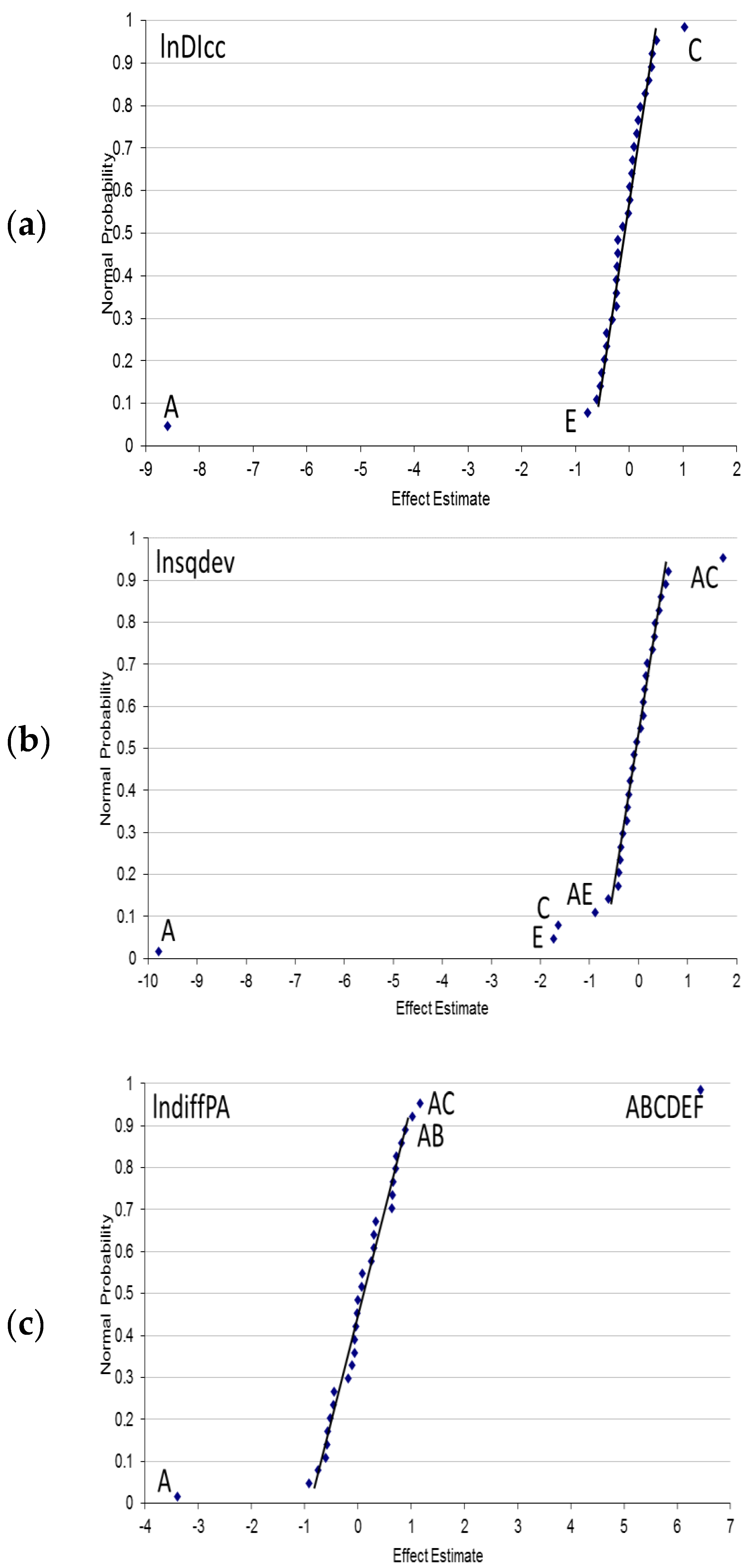
Figure 6 provides the normal probability plots for lnDIcc, lnsqdev, and lndiffPA in the half-fraction factorial design using only 32 runs. Once again, effects that are labeled (using labels from Table 1) denote reasonably large effects. As previously mentioned, the five-way interactions were aliased with main effects and the two-way interactions were aliased with four-way interactions (Table 3). For lnDIcc, the main effects for (A) the transmitter angle, (C) frequency, and (E) distance to excitation, appeared large and were worth exploring, which was consistent with the full factorial design. As previously mentioned, five-way interactions were aliased with the main effects, but were considered negligible. Therefore, we attributed the large effects in the normal probability plot for lnDIcc in the half-fraction factorial to that of the main effects instead of the associated five-way interaction. This finding was confirmed when running the ANOVA, as the runs included in the half-fraction factorial (Table 5). (A) The transmitter angle, (C) frequency, and (E) distance to excitation were all significantly related to lnDIcc (p-values < 0.0001, 0.0002, 0.0065, respectively). Consistent with the full factorial design, the model R2 value was 0.97 (RMSE = 0.8993).
Similarly, for the half-fraction factorial design, the main effects of transmitter angle (A), frequency (C) and distance to excitation (E) as well as the two-way interactions of transmitter angle with frequency (AC) and transmitter angle with distance to excitation (AE) appear large in the normal probability plot for lnsqdev (Figure 6). Here in the half-fraction factorial, the two-way interactions are aliased with the four-way interactions. However, we assume that the higher order interactions are negligible and once again, attribute the larger effects to the two-way interactions instead. The results for lnsqdev in the half-fraction factorial (Table 5) are also analogous to that from the full factorial design and the ANOVA conducted on these 32 runs resulted in a comparable R2 = 0.97 (RMSE = 0.9992) with significant p-values for the transmitter angle/distance to excitation interaction (p-value = 0.0039), transmitter angle/frequency interaction (p-value = 0.0019).
Finally, we notice some differences with respect to the significant factors apparent in the normal probability plot for lndiffPA from the half-fraction factorial (Figure 6). First, the six-way interaction appears to have the largest effect, yet because of our assumptions, we will not focus on modeling this interaction. Instead, we examine the remainder of the plot and notice that transmitter angle has the most noticeable negative effect (Figure 6). The other effects do not seem overly large, although the only two other effects over 1.0 are noted: the interaction of transmitter angle with receiver angle (AB) and with frequency (AC). However, consistent with the full factorial design, the error in this model is larger and effects in the normal probability plot are less pronounced. Examining the resulting ANOVA from this half-fraction design for lndiffPA using only transmitter angle results in a significant effect (p-value< 0.0001) for transmitter angle and transmitter angle is found to explain 64.7% of the variation observed in lndiffPA (R2 = 0.6468, RMSE = 1.4624).

4. Discussion

The physical constraints in structures did not always allow optimal SHM configuration for monitoring, especially in hot spot monitoring. Knowing how alternation in the SHM configuration would affect the response was paramount to collecting and detecting quality data from which to determine whether structural cracks were forming, especially for critical structures and components. The factorial design that was utilized here was able to determine, among the SHM configuration settings, which factors were the most sensitive and produced the largest variation in the calculated damage index. By conducting these results in the simulation environment, we could save substantial costs and better inform subsequent experiments by using real material, which could focus on other factors. Furthermore, multiple damage indices could be computed and compared in order to determine which were the most robust to damage detection within the configuration. Later, if there were other damage indices that were of interest, the simulation data that were collected could be reprocessed in order to provide the same analysis for the new indices. In this manner, we could always build upon this data that were collected and reduce the need to re-run experiments, especially in samples, each time the damage index or other features were changed.
The ability of an SHM system to accurately detect and monitor damage was dependent upon the modality, physical configuration, damage indices, and features processed from the resulting signals, as well as other environmental and application specific determinants. We assumed that the application was a known PWAS in an aluminum plate and initiated the study with an examination of the sensitivity of various configuration and sensing parameters, as well as potential damage indices computable from the resultant signals. The choice of values that were given to these parameters during the SHM design had been, in the past, rather subjective. In this work, we showed that this choice did not need to be purely subjective; we demonstrated that this choice could be objectively made using the concept of sensitivity and tested with an appropriate statistical design. This current study used a binary (low/high) value assignment to each of the six parameters that were examined (namely, transmitter angle, receiver angle, frequency of excitation, sensor size, distance between excitation, and damage site and flaw size). The choice of the values that we assigned to the low and high levels of each of these factors was based upon many considerations, including the following: (1) physical options of sensor layout on a realistic riveted lapjoint; (2) our professional experience in designing SHM systems; (3) the tuning effects between guided waves and PWAS transducers; and (4) the effect of wave attenuation with distance from the point source as its energy spreads in ever increasing wavefront circles. Although the values we chose might appear somewhat subjective, we were able to determine major trends with respect to these effects on the SHM response and clearly demonstrated how such studies, which started in the simulation environment, might be able to inform subsequent studies.
The results from our analysis provided the researcher with valuable information, prior to tests in material or real structures, regarding how to best produce a response, as well as which summary measures (damage indices) of a signal were best suited for the geometry of the proposed SHM. The transmitter angle had by far the response signal, followed by the frequency and distance between excitation and the transmitter angle. These were the most critical components of the SHM system that we examined, and were logical given the geometry and considerations mentioned above, as well as the damage indices themselves, which were computed as comparisons of the baseline (no damage) signal to that of the signal in the damage state.
The SHM parameters that were significant for the damage index, based upon the correlation coefficient, contained no interactions, whereas interactions were present for the sum of the squared deviations between the baseline and observed signal. The lack of interaction for the correlation coefficient damage index was reasonable, since the correlation coefficient was scaled by the squared deviations and was perhaps a more robust measure for the SHM system. These results suggested that if the hot spot would not allow for a small transmitter angle, we still might have been able to invoke a larger response by decreasing the distance to the excitation, or, if these configuration changes were not possible, by exciting at a higher frequency. Similar responses could be achieved if using the sum of the squared deviations, however, the combined effects of the transmitter angle with frequency and distance to excitation would have to be taken into account. The difference in the peak amplitude damage index did not account for differences across the entire signal. Although simple to compute, its loss of information that was embedded in the rest of the signal was evident in its lower R2 value and the inconsistencies between the full factorial and half-fraction factorial statistical designs. When considering the use of a sensitive damage index, the difference in the peak amplitude remained less sensitive than the other indices that were considered.
It was, perhaps, surprising that the flaw size was not significant. However, the lack of sensitivity with respect to the sensor size had been observed previously [12]. Clearly, the flaw size must have had some effect, otherwise there would have been no differences between the signals. It was possible that the range of flaw sizes, and in particular the smallest flaw size, was actually quite large for this application and therefore could explain why no significant effects were found. In fact, the associated wavelengths in this material (31.2 mm and 11.3 mm for 200 kHz and 550 kHz frequencies, respectively) were large in relation to the difference in crack length. Therefore, in relation to the other factors that we examined, we deduced that, although the system was sensitive to the existence of damage, it might not have had the sensitivity required to determine the size of the damage in the range that we examined. We expected that these results would change when smaller flaw sizes were considered. Finally, with respect to the parameters chosen and their results, we noted that in choosing binary low/high values, we assumed a linear trend across the values of the various parameters. If it was thought that these trends might have been be curvilinear, then three (low, medium, and high) or more values would be important. The statistical designs that include such levels did exist, as described below. In fact, we intend to address these issues in possible future work.
With respect to the statistical designs, although we focused on a specific factorial design, other designs did exist. The usefulness of the factorial design was in its ability to save experimental runs and cost by collapsing the design into half of the runs that were required to consider all of the experimental settings. In general, we demonstrated comparable results using only half of the runs in the half-fraction factorial design and we then demonstrated the efficiency of using such a design. One potential draw-back of the 2k design was in the inference between the two settings of each parameter. Since we only used two such settings, we assumed a linear trend across values of each of the various parameters (see Figure 5 for instance). This assumption might not have held in all design settings. However, there were other factorial designs, for instance 3k factorial designs, which considered a general high, medium, and low level for each factor. If it was thought that the response might have been curvilinear as the value of the parameter increased/decreased, then the 3k design could be used to model this curvilinear trend from low to high. With such designs, the trends in the parameter values could be examined while still reducing the number of runs that were required (e.g., a half-fraction for the 3k design was possible). Such a reduction in the number of experiments was especially important considering that a 26 design was 64 experimental runs, but a full 36 design was 729 experimental runs.
It is noteworthy to remark that for the lndiffPA damage index, the normal probability plot in the half-fraction design was not as clear as is was for the other damage indices, which would be expected because of its lower sensitivity as a damage index. The plot did pick up, though, on the largest effect for lndiffPA, that being the transmitter angle. Admittedly, there was no hard and fast rule that stated that only the large effects that were found on the normal probability plot should have been be used in the ANOVA setting, as we did here. In general, this approach worked well and had produced, in both the full factorial and in a reduced design, the main significant effects for each damage index. However, the ANOVA could be conducted without this first step. In fact, if we fitted the ANOVA using a model building approach that would remove the non-significant, higher order interactions for lndiffPA, we found, as a stopping point, that the three-way interaction between the transmitter angle, receiver angle, and frequency (ABC) was significant for lndiffPA (R2 = 0.78). However, we utilized the normal probability plots in the spirit of the sparsity of effects principle and in order to establish appropriate degrees of freedom. As such, from only the half-fraction results, we concluded that if the damage index lndiffPA was of interest, further work would be needed in order to identify additional sources of variation—A result that might have also been concluded from the full factorial design, given the lower comparative R2 value. In fact, as we conducted the comparison of the damage indices to determine which were the most sensitive and robust for the SHM system, our conclusion was to work with either the damage index, based upon the correlation coefficient, or the sum of the squared deviations, as lndiffPA was much less predictive. This was a conclusion that was determined by the half-fraction factorial design. Furthermore, an R2 of about 97% was achievable with the correlation coefficient damage index and no interactions were present, demonstrating that this damage index was more malleable and robust for this SHM system.
Finally, we did not intend for this work to suggest that the system configuration should be determined based upon the damage index. Instead, we used different damage indices as a summary of the response signals, in order to demonstrate their ability to sensitively pick up the change in the signal, resulting from the presence of a crack, as not all damage indices were able to mathematically capture the nuances in the signal that were a result from the physics of the configuration and the damage that was present.

5. Conclusions

In conclusion, there is much utility when using the simulation modeling environment to determine the SHM sensitive factors that must be considered in subsequent experiments. Furthermore, with care in choosing the statistical design, an efficient and reduced number of experimental runs can provide the same information as a full experiment containing all of the factor levels that are varied simultaneously. We have found that the transmitter angle is the most sensitive SHM configuration design setting that is influential on the SHM response. Furthermore, some damage indices are more sensitive than others. The correlation coefficient appears to be the most robust as, although it is sensitive to the transmitter angle, frequency, and distance to excitation, these factors can be varied separately, as the correlation coefficient was not sensitive to interactions among these factors as the sum of squared deviations was. Furthermore, if carefully accounting for these factors, about 97% of the variation in the response can be explained. The sensor size and flaw sizes considered in this study are not significant and have no large effect on the response. In addition, choosing a simple damage index, such as the difference in the peak amplitude, results in a fair amount of variation in the response (about 30%) that is unexplained, which perhaps makes it the least useful damage index that we examined, producing inconsistent statistical results, as demonstrated by the full and half-fraction factorial statistical designs.
Finally, the methodologies and framework used in this study have larger implications for effective design and uncertainty evaluation in the design of structural health monitoring systems. With planning and care, results from a study such as this can be used to inform a subsequent experiment examining a secondary set of factors, which would build upon the these results. By reducing the number of data runs and testing the parameters in simulation environments, where possible, a sequential approach to quantifying the sensitivity of the SHM system to all observable factors may be constructed, enabling a cost- and time-efficient approach to the demonstration of the SHM system validation.

Acknowledgments

This research was partially supported by a grant from the Air Force Office of Scientific Research (AFIT Research Support Fund 17C273C). The views expressed herein are those of the authors and do not reflect the official policy or position of the United States Air Force, Department of Defense, or the United States Government.

Author Contributions

Victor Giurgiutiu, Bin Lin, and Christine Schubert Kabban conceived and designed the experiments; Richard Uber theorized the experimental configuration and he and Kevin Lin coded and performed the experiments; Md Yeasin Bhuiyan and Bin Lin consulted and provided the base code for the experimentation; Kevin Lin and Christine Schubert Kabban processed and analyzed the data; Christine Schubert Kabban wrote the paper; and all of the authors provided appropriate background and editorial remarks.

Conflicts of Interest

The authors declare no conflict of interest. The founding sponsors had no role in the design of the study; in the collection, analyses, or interpretation of data; in the writing of the manuscript; or in the decision to publish the results.

References

  1. Derriso, M.M.; Olson, E.E.; DeSimio, M.P. Military Aircraft. In Encyclopedia of Structural Health Monitoring; Boller, C., Change, F.-K., Fujino, Y., Eds.; Wiley Blackwell: Hoboken, NJ, USA, 2009; Volume 1. [Google Scholar] [CrossRef]
  2. Department of Defense. Aircraft Structural Integrity Program General Guidelines; MIL-STD-1530D (USAF); Department of Defense: Arlington County, VA, USA, 2016.
  3. Condition Based Maintenance Plus (CBM+). CBM+ Plan. 2013. Available online: http://www.acq.osd.mil/log/mpp/.cbm+.html/CBM+_Plan2013v2.pdf (accessed on 12 February 2018).
  4. Lindgren, E.A.; Knopp, J.S.; Aldrin, J.C.; Steffes, G.J.; Buynak, C.F. Aging aircraft NDE: Capabilities, challenges, and Opportunities. AIP Conf. Proc. 2007, 894, 1731. [Google Scholar] [CrossRef]
  5. Janapati, V.; Kopsaftopoulos, F.; Li, F.; Lee, S.J.; Chang, F.K. Damage detection sensitivity characterization of acousto-ultrasound-based structural health monitoring techniques. SHM 2016, 15, 143–161. [Google Scholar] [CrossRef]
  6. Masserey, B.; Fromme, P. Analysis of high frequency guided wave scattering at a fastener hole with a view to fatigue crack detection. Ultrasonics 2017, 76, 78–86. [Google Scholar] [CrossRef] [PubMed]
  7. Zeng, L.; Lin, J.; Bao, J.; Joseph, R.P.; Huang, L. Spatial resolution improvement for Lamb wave-based damage detection using frequency dependency compensation. J. Sound Vib. 2017, 394, 130–145. [Google Scholar] [CrossRef]
  8. Stawiarski, A.; Barski, M.; Pajak, P. Fatigue crack detection and identification by the elastic wave propagation method. Mech. Syst. Signal Process. 2017, 89, 119–130. [Google Scholar] [CrossRef]
  9. Hong, M.; Su, Z.; Lu, Y.; Sohn, H.; Qing, X. Locating fatigue damage using temporal signal features of nonlinear Lamb waves. Mech. Syst. Signal Process. 2015, 60–61, 182–197. [Google Scholar] [CrossRef]
  10. Ihn, J.B.; Chang, F.K. Pitch-catch active sensing methods in structural health monitoring for aircraft structures. SHM 2008, 7, 5–19. [Google Scholar] [CrossRef]
  11. Fendzi, C.; Morel, J.; Rebillat, M.; Guskov, M.; Mechbal, N.; Coffignal, G. Optimal sensors placement to enhance damage detection in composite plates. In Proceedings of the 7th European Workshop on Structural Health Monitoring, Nantes, France, 8–11 July 2014; Curran Associates: Red Hook, NY, USA, 2014; pp. 1–8. [Google Scholar] [CrossRef]
  12. Raghavan, A.; Cesnik, C.E.S. Finite-dimensional piezolelectric transducer modeling for guided wave based structural health monitoring. Smart Mater. Struct. 2005, 14, 1448–1461. [Google Scholar] [CrossRef]
  13. Lu, Y.; Michaels, J.E. Feature extraction and sensor fusion for ultrasonic structural health monitoring under changing environmental conditions. IEEE Sens. J. 2009, 9, 1462–1471. [Google Scholar] [CrossRef]
  14. Kopsaftopoulos, F.P.; Fassois, S.D. A functional model based statistical time series method for vibration based damage detection, localization, and magnitude estimation. Mech. Syst. Signal Process. 2013, 39, 143–161. [Google Scholar] [CrossRef]
  15. Kopsaftopoulos, F.P.; Fassois, S.D. Vibration based health monitoring for a lightweight truss structure: Experimental assessment of several statistical time series methods. Mech. Syst. Signal Process. 2010, 24, 1977–1997. [Google Scholar] [CrossRef]
  16. Roy, S.; Ladpli, P.; Lonkar, K.; Chang, F.K. Structural damage detection using ultrasonic guided waves under varying ambient temperature and loading environments. In Proceedings of the 9th IWSHM, Stanford, CA, USA, 10–12 September 2013; pp. 1284–1293. [Google Scholar]
  17. Roy, S.; Lonkar, K.; Janapati, V.; Chang, F.K. A novel physics-based temperature compensation model for structural health monitoring using ultrasonic guided waves. SHM 2014, 13, 321–342. [Google Scholar] [CrossRef]
  18. Moriot, J.; Quaegebeur, N.; Le Duff, A.; Masson, P. A model-based approach for statistical assessment of detection and localization performance of guided wave-based imaging techniques. SHM 2017, 1–13. [Google Scholar] [CrossRef]
  19. Gianneo, A.; Carboni, M.; Giglio, M. Feasibility study of a multi-parameter probability of detection formulation for a lamb waves-based structural health monitoring approach to light alloy aeronautical plates. SHM 2016, 16, 225–249. [Google Scholar] [CrossRef]
  20. Giurgiutiu, V.; Zagrai, A.; Bao, J.J. Piezoelectric wafer embedded active sensors for aging aircraft structural health monitoring. SHM 2002, 1, 41–61. [Google Scholar] [CrossRef]
  21. Shen, Y. Structural Health Monitoring Using Linear and Nonlinear Ultrasonic Guided Waves. Ph.D. Thesis, University of South Carolina, Columbia, SC, USA, 2014. [Google Scholar]
  22. Bhuiyan, M.Y.; Shen, Y.; Giurgiutiu, V. Interaction of Lamb waves with rivet hole cracks from multiple directions. Proc. Inst. Mech. Eng. Part C J. Mech. Eng. Sci. 2017, 231, 2974–2987. [Google Scholar] [CrossRef]
  23. Giurgiutiu, V. Structural Health Monitoring with Piezoelectric Wafer Active Sensors, 2nd ed.; Elsevier: Waltham, MA, USA, 2014; ISBN 978-0-12-418691-0. [Google Scholar]
  24. Shen, Y.; Giurgiutiu, V. WaveFormRevealer 1-D—An Analytical Predictive Tool for the 1-D Simulation of Multimodal Guided Waves Propagation and Interaction with Damage: User’s Guide and Theoretical Foundation; Report # USC-ME-LAMSS-2012-101; University of South Carolina: Columbia, SC, USA, 2012. [Google Scholar]
  25. Shen, Y.; Giurgiutiu, V. Effective non-reflecting boundary for Lamb waves: Theory, finite element implementation, and applications. Wave Motion 2015, 58, 22–41. [Google Scholar] [CrossRef]
  26. Bhuiyan, M.Y.; Shen, Y.; Giurgiutiu, V. Guided wave based crack detection in the rivet hole using global analytical with local fem approach. Materials 2016, 9, 602. [Google Scholar] [CrossRef] [PubMed]
  27. Shapiro, S.S.; Wilk, M.B. An analysis of variance test for normality (complete samples). Biometrika 1965, 52, 591–611. [Google Scholar] [CrossRef]
  28. Montgomery, D.C. Design and Analysis of Experiments, 3rd ed.; John Wiley and Sons: New York, NY, USA, 1991; ISBN 0-471-52000-4. [Google Scholar]
  29. Daniel, C. Use of half-normal plots in interpreting factorial two level experiments. Technometrics 1959, 1, 311–342. [Google Scholar] [CrossRef]
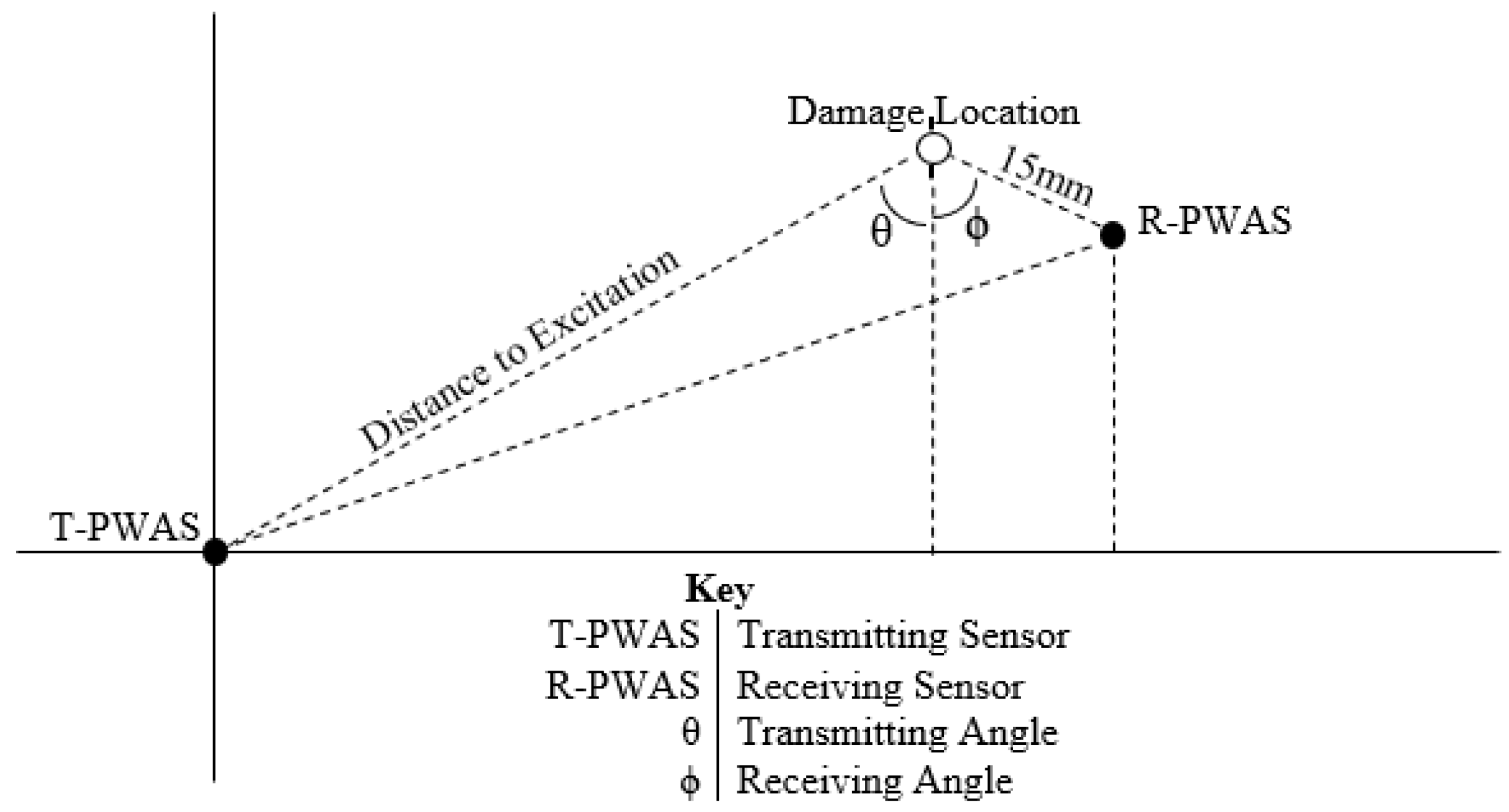
Figure 1. Numerical simulation modeling the experimental configuration. R-PWAS—receiving piezoelectric wafer active sensor; T-PWAS—transmitting piezoelectric wafer active sensor.
Aerospace 05 00045 g001
Figure 2. Computational domain of the rivet hole for the finite element method (FEM): (a) overall FEM model; (b) zoomed in at the damage region (there are two nodes disbanded along the crack); and (c) boundary conditions applied along the loading line, where the stress mode shapes were converted into the nodal force that was applied at each node.
Aerospace 05 00045 g002
Figure 3. Normal probability plots from the full factorial experiment for each damage index: (a) normal probability plot for the natural log of the correlation coefficient damage index (lnDIcc); (b) normal probability plot for the natural log of the sum of squared deviations (lnsqdev); and (c) normal probability plot for the natural log of the difference in peak amplitude (lndiffPA). A—transmitter angle; B—receiver angle; C—frequency; D—sensor size; E—excitation distance; F—flaw size.
Aerospace 05 00045 g003
Figure 4. Estimated responses and associated 95% confidence intervals for the correlation coefficient damage index (DIcc) at each level of transmitter angle, frequency, and distance between excitation and transmitter.
Aerospace 05 00045 g004
Figure 5. Estimated responses and associated 95% confidence intervals for the natural log of the sum of squared deviations (lnsqdev) at the following: (a) the interaction of transmitter angle with distance to excitation; (b) the interaction of transmitter angle with frequency; (c) for the natural log of the difference in peak amplitude (lndiffPA) at the interaction of transmitter angle and frequency fixed at a receiver angle of 5 degrees; and (d) a receiver angle of 20 degrees.
Aerospace 05 00045 g005
Figure 6. Normal probability plots from the half-fraction factorial experiment for each damage index: (a) normal probability plot for the natural log of the correlation coefficient damage index (lnDIcc); (b) normal probability plot for the natural log of the sum of squared deviations (lnsqdev); and (c) normal probability plot for the natural log of the difference in peak amplitude (lndiffPA).
Aerospace 05 00045 g006
Table 1. Experimental factors and levels.
LabelFactorGeneric LevelSpecific Values
ATransmitter Angle, θLow
High27°
BReceiver Angle, φLow
High20°
CFrequencyLow200 kHz
High550 kHz
DSensor SizeLow5 mm
High7 mm
EDistance between Excitation and Damage SiteLow150 mm
High250 mm
FFlaw SizeLow0.64 mm
High3.20 mm
Table 2. Low (L) and high (H) factor level settings for the 26 experimental runs.
RunABCDEF
Transmitter AngleReceiver AngleFrequencySensor SizeDistance to ExcitationFlaw Size
1LLLLLL
2HLLLLL
3LHLLLL
4HHLLLL
.....................
63HHHHHL
64HHHHHH
The actual values that were used for the High (H) and Low (L) settings are given in Table 1.
Table 3. Aliased effects in the 26−1 resolution VI half-fraction factorial design.
Factors for the Half-Fraction Factorial Design (and Associated Aliased Factor)
A = BCDEFAB = CDEFBD = ACEFDE = ABCFABC = DEFACF = BDE
B = ACDEFAC = BDEFBE = ACDFDF = ABCEABD = CEFADE = BCF
C = ABDEFAD = BCEFBF = ACDEEF = ABCDABE = CDFADF = BCE
D = ABDEFAE = BCDFCD = ABEF ABF = CDEAEF = BCD
E = ABCDFAF = BCDECE = ABDF ACD = BEF
F = ABCDEBC = ADEFCF = ABDE ACE = BDF
A—transmitter angle; B—receiver angle; C—frequency; D—sensor size; E—excitation distance; F—flaw size.
Table 4. Full factorial design ANOVA model and R2 results by each damage index.
FactorlnDIcc lnsqdev lndiffPA
Sums of Squaresdfp-Value Sums of Squaresdfp-Value Sums of Squaresdfp-Value
A1166.461<0.0001 1518.101<0.0001 164.571<0.0001
B--- --- 12.1810.0030
C21.811<0.0001 38.051<0.0001 3.2210.1180
E10.6810.0002 54.861<0.0001 ---
AE--- 10.851<0.0001 ---
AC--- 41.971<0.0001 23.581<0.0001
AB--- --- 24.961<0.0001
BC--- --- 0.1410.7440
ABC--- --- 24.011<0.0001
Error39.6160 36.2358 71.6656
Total1238.5663 1700.0763 324.2563
R20.9680 0.9787 0.7790
RMSE0.8125 0.7903 1.1312
A—transmitter angle; B—receiver angle; C—frequency; D—sensor size; E—excitation distance; F—flaw size; df—degrees of freedom; lnDIcc—natural log of the correlation coefficient damage index; lnsqdev—natural log of the sum of squared deviation; lndiffPA—natural log of the difference in peak amplitude.
Table 5. Half-fraction factorial design ANOVA model and results by each damage index.
FactorlnDIcc lnsqdev lndiffPA
Sums of Squaresdfp-Value Sums of Squaresdfp-Value Sums of Squaresdfp-Value
A608.681<0.0001 834.341<0.0001 117.511<0.0001
C14.8010.0002 15.8610.0016 ---
E7.0010.0065 23.451<0.0001 ---
AE--- 5.9610.0039 ---
AC--- 6.3710.0019 ---
Error22.6428 25.9626 64.1630
Total653.1231 911.9331 181.6731
R20.9653 0.9736 0.6468
RMSE0.8993 0.9992 1.4642
A—transmitter angle; B—receiver angle; C—frequency; D—sensor size; E—excitation distance; F—flaw size; df—degrees of freedom; lnDIcc—natural log of the correlation coefficient damage index; lnsqdev—natural log of the sum of squared deviation; lndiffPA—natural log of the difference in peak amplitude.