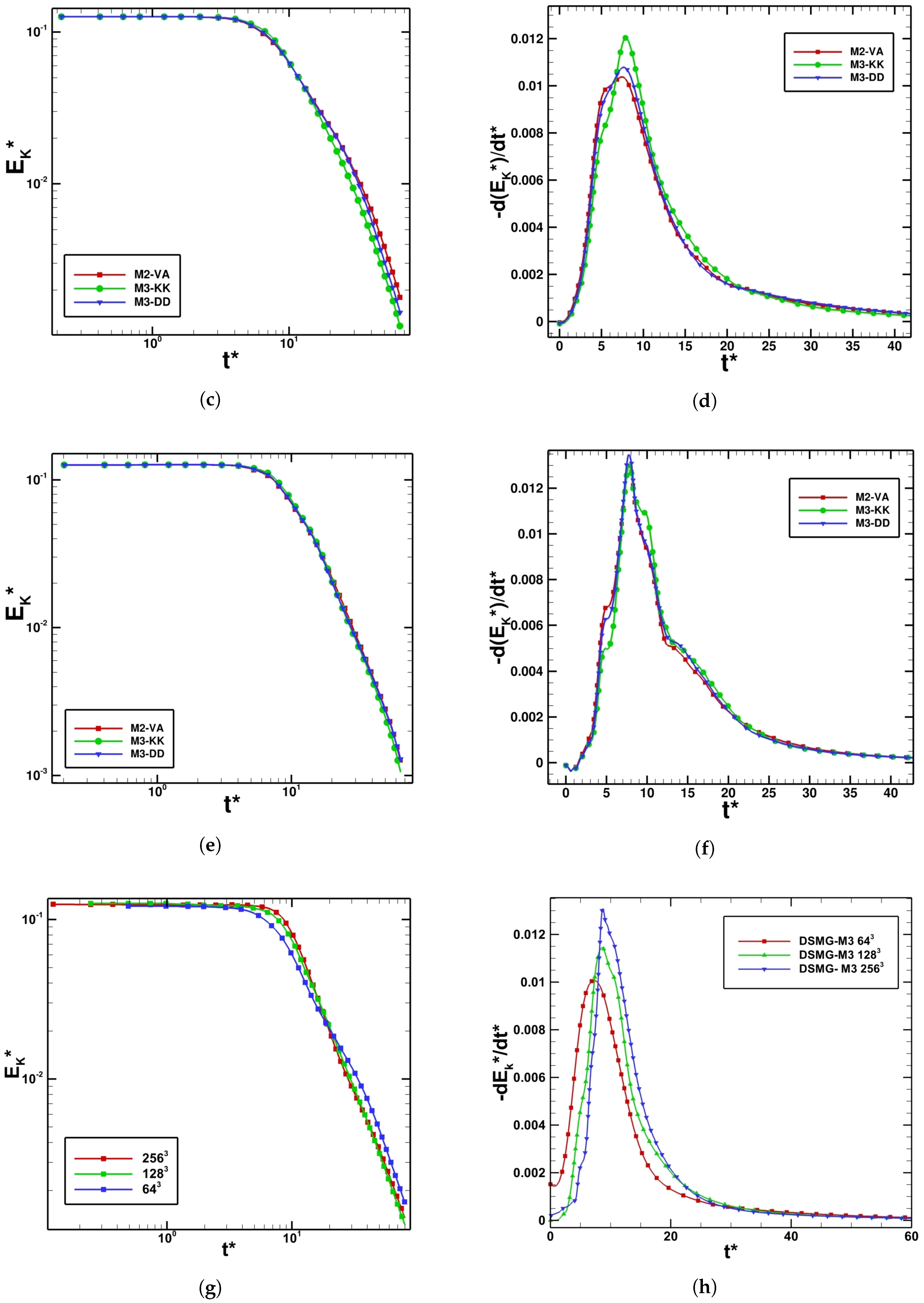
3.2. Effect of Grid Resolution
The dynamics of the Taylor–Green vortex are directly dependent on the resolving power of the numerical scheme and the grid size adopted. In order to assess the effect of grid resolutions on the evolution of TGV flow, simulations were performed using second and third-order MUSCL schemes (M2-VA, M3-KK and M3-DD) considering three levels of grids having sizes of
,
and
cells. It should be noted that the second-order strong-stability preserving Runge–Kutta scheme has been utilized for temporal discretisation. The same grid refinement study was performed using the dynamic Smagorinsky subgrid-scale model and third-order MUSCL scheme (DSMG-M3) on
,
and
grids. The differences in the flow dynamics during the time evolution of the simulation are of great interest to understand the effect of mesh size on the performance of the numerical scheme or the SGS model.
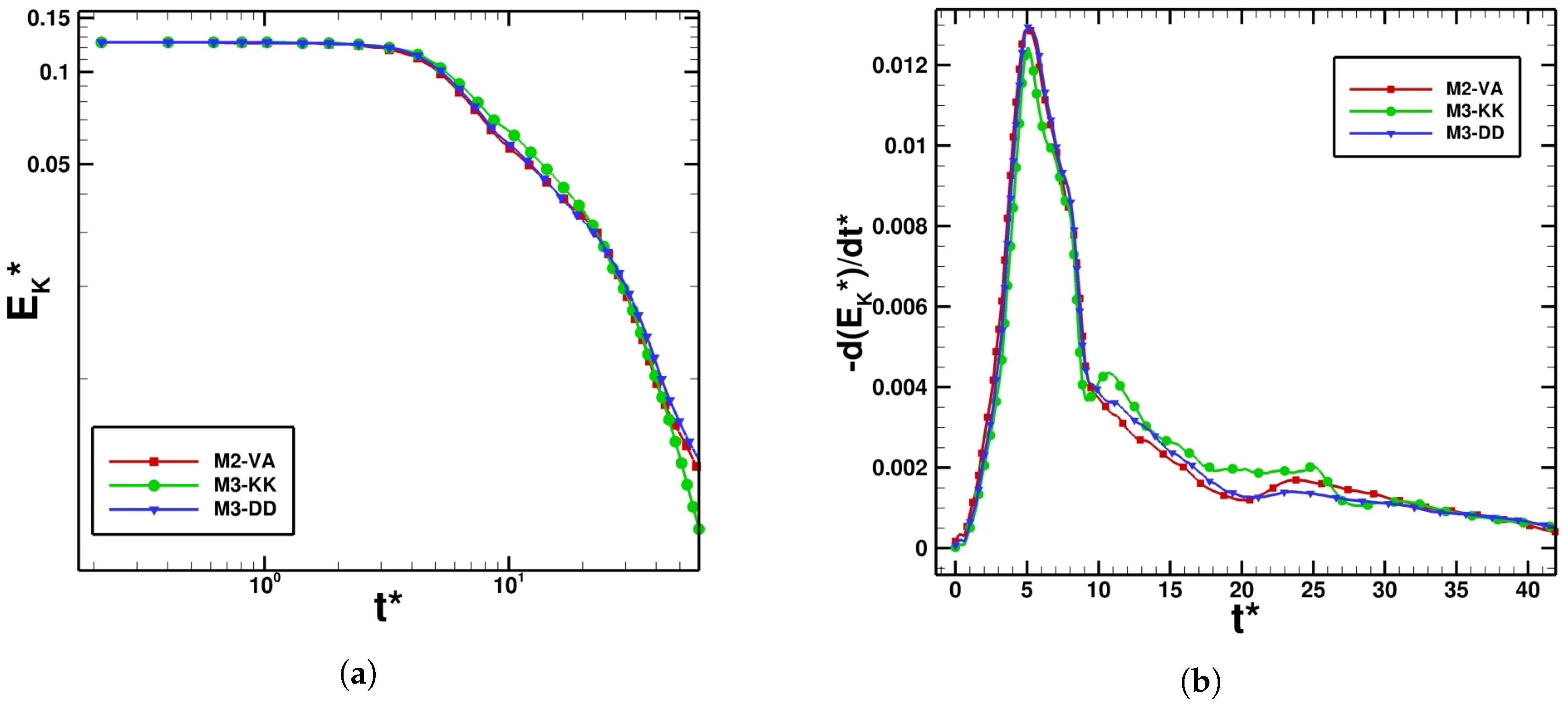
Figure 3 shows the evolution of volumetrically-averaged dimensionless kinetic energy and kinetic energy dissipation rate for all the numerical methods and all grid levels used within this study.
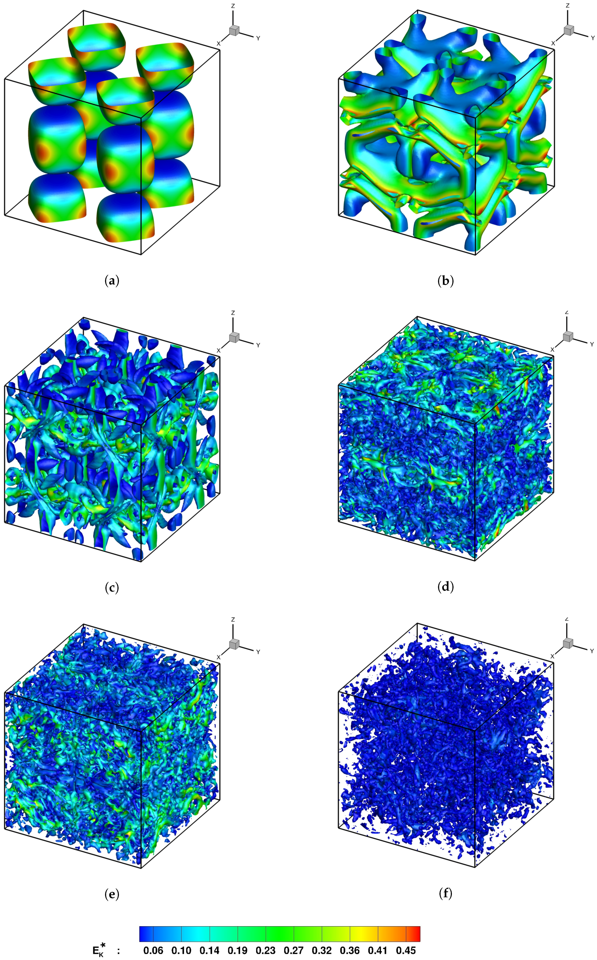
The kinetic energy is represented in logarithmic scale to understand the trend line that the kinetic energy decay follows. In theory, the kinetic energy for an inviscid flow should be conserved since no viscous effects are present to damp it into heat. However, it is obvious that the latter is decaying during the coarse of the simulations. The decay starts at the end of the laminar stage when the vortex sheet is generated and the flow becomes under-resolved. The kinetic energy dissipation increases due to the instability that the vortex sheet undergoes and to the formation of a smaller and smaller vortical tube. The DNS study performed by Brachet et al. [
20,
21] predicted that the kinetic energy reaches its dissipation peak at a non-dimensional time level
. The time level at which the dissipation reaches its highest value is more or less predicted correctly by all the numerical schemes with the exception of DSMG-M3, which underpredicted that time level compared to the other schemes. At a time level higher than
, the kinetic energy dissipation decreases rapidly and reaches a value of zero at very late time stages, and this behaviour is similar to homogeneously-decaying turbulence. The kinetic energy dissipation rate trend obtained on the
mesh shows a non-physical behaviour predicted by all the numerical schemes used within the framework of the ILES approach. At late stages, when the flow becomes highly-disorganized (
), all the numerical schemes predicted an increase in the dissipation of kinetic energy, which created a sort of hump in the trend of
. In addition to that, the M3-KK scheme predicted an earlier increase in the kinetic energy dissipation at
, which indicates a lower resolving power of that scheme compared to the other methods. Using finer grid resolutions, this non-physical behaviour vanishes, and the decay of kinetic energy at the stages when the flow is fully disorganized is pretty smooth. One could observe that this non-physical trend of kinetic energy dissipation rate was not observed in LES even on the coarsest grid. The dissipation peak represented by DSMG-M3 on a 64
mesh appears prior to the peak predicted on finer grids, which indicates that the onset of kinetic energy dissipation is happening earlier on a 64
grid. Refining the mesh, the kinetic energy plot represented in
Figure 3g is more conserved since the volumetrically-averaged kinetic energy decay starts later on 128
and 256
grids compared to the coarsest grid, as observed qualitatively. The conclusion that could be drawn from the observation of kinetic energy and the kinetic energy dissipation rate is that the resolving power of the numerical scheme increases using finer grid resolutions. Note that mesh refinement increases the computational cost, which might become quite expensive for very fine grid resolutions. Both the ILES and LES approaches predicted similar dynamics of TGV, which indicates that the numerical dissipation inherent in high-order non-oscillatory numerical schemes could act as an implicit subgrid-scale model in predicting the flow features of homogeneously-decaying turbulence. As mentioned earlier, the kinetic energy
is represented in a logarithmic scale in order to understand the trend line of the evolution of kinetic energy in time. It is obvious from
Figure 3a,c,e,g that the kinetic energy follows a power law in time. This trend is similar to homogeneous and isotropic turbulence, where Kolmogorov [
28] showed that the kinetic energy decay obeys a power law in time as:
where
represents the onset of kinetic energy decay and
P is the power that was evaluated by Kolmogorov and equal to
. If the length of the largest scales of motion present in the flow are comparable to the grid resolution, the kinetic energy decays following a power law with
, as shown in [
33]. In this study, the decay exponent
P is determined using curve fitting of kinetic energy data between
and
and values obtained for all numerical methods (see
Table 1 and
Table 2).
The decay exponent predicted by the numerical schemes used within the ILES approach on
and
grids falls in the range of the value predicted in [
33] (
). The value of
P is underpredicted by all the numerical methods on the coarsest mesh (
cells), and it was similar to the value of the decay exponent predicted for homogeneous turbulence by Kolmogorov [
28]. However, even if the values of
P predicted by the coarsest mesh are close to the decay exponent of homogeneous and isotropic turbulence, one should not forget that a non-physical hump was observed in the volumetrically-averaged kinetic energy evolution, which makes the prediction of the decay slope erroneous. Without the presence of this “artificial” hump, the slope of decay would be steeper, and that could explain why the value of
P was underpredicted. Refining the mesh, the hump vanishes, and the decay exponent converges to a value similar to the theoretical value provided by Skrbek and Stalp [
33]. In regards to LES, it is obvious that the decay exponent obtained on a
grid is lower than the slope predicted by the medium and fine mesh, which converges to two.
The onset is a very important parameter to understand and examine the resolving power of each numerical scheme. The more the kinetic energy is conserved, or in other words, the higher the onset of decay, the better the scheme is in terms of performance. It is obvious from
Table 1 that M2-VA starts loosing kinetic energy before M3-DD, and the latter looses energy before M3-KK, which predicts the highest decay onset. Refining the mesh, the kinetic energy is more conserved, and hence, the performance of the numerical scheme is increased. The time at which the kinetic energy starts to decay is shown in
Table 2 for the LES. Large differences of decay onset between the coarse, medium and fine grids are clear, and that could explain why the peak in the energy dissipation on the
grid appears earlier in
Figure 3h. Refining the mesh, the onset of decay increases significantly and reaches a value of 4.296 on the
mesh, which indicates that the kinetic energy is best conserved on the finest grid. Compared to ILES results on a
grid, the onset of decay predicted by LES is nearly half the values predicted by all numerical schemes (see
Table 1), which means that DSMG-M3 looses kinetic energy faster than the high-order non-oscillatory finite volume numerical schemes used for ILES, and the flow becomes under-resolved earlier as predicted by DSMG-M3.
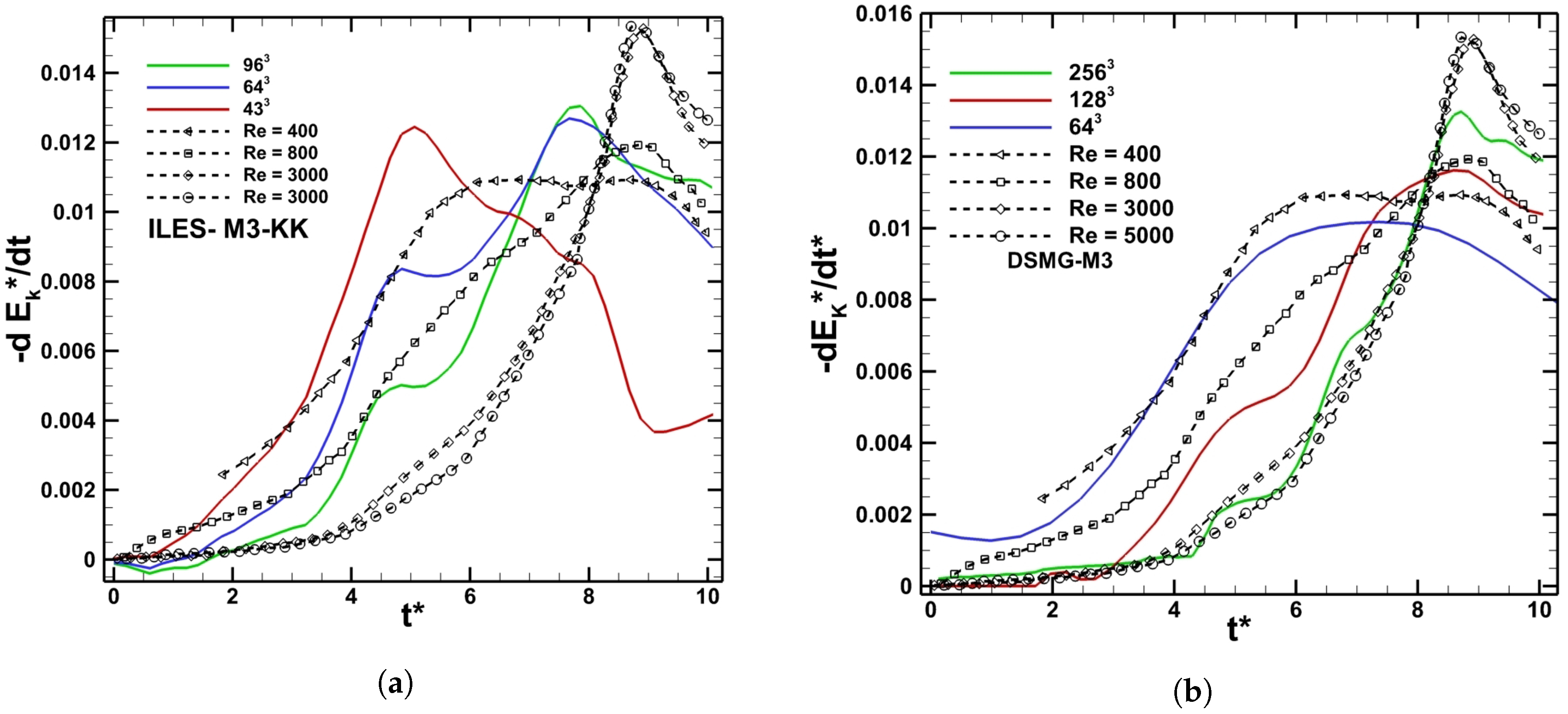
Studies of grid sensitivity of ILES and LES were carried out on all the grids generated and compared to DNS data provided in the study of Brachet et al. [
20,
21] for Re
, 800, 3000 and 5000. It should be noted that explicit data for different Reynolds numbers are not available for the ILES and LES approaches, but the trend of kinetic energy dissipation rate will be used to observe the evolution of kinetic energy dissipation, as will be presented in
Figure 4, compared to DNS results, which present the effects of physical viscosity, which damps the kinetic energy into heat. The DNS study showed that at high Reynolds number (Re
), the peaks of the kinetic energy dissipation rate remain identical, which means that the dissipation of kinetic energy reaches a Reynolds independent limit. By increasing the Reynolds number above this limit, the dissipation of kinetic energy will have the same trend. This concept is examined in the context of this study where the evolution of kinetic energy dissipation increases the investigated grid resolutions to examine which Reynolds number trends the implicit and explicit numerical viscosities are predicting. Only the results obtained using DSMG-M3 and M3-KK are presented since they are representative of all trends of numerical schemes.
Finer grid resolutions correspond to lower kinetic energy dissipation and higher Reynolds number trends. Reynolds-dependent effects are clear from the evolution of the dissipation peak when using coarser grids. The Reynolds number independent effect was clearer on the 256 grid used to perform the LES, where the trend of kinetic energy dissipation rate follows the high Reynolds number data, and the peak is reaching the value predicted for Re and 5000, respectively. Hence, implicit and explicit subgrid-scale viscosities will predict a sort of Reynolds number independent limit when refining the grid resolution.
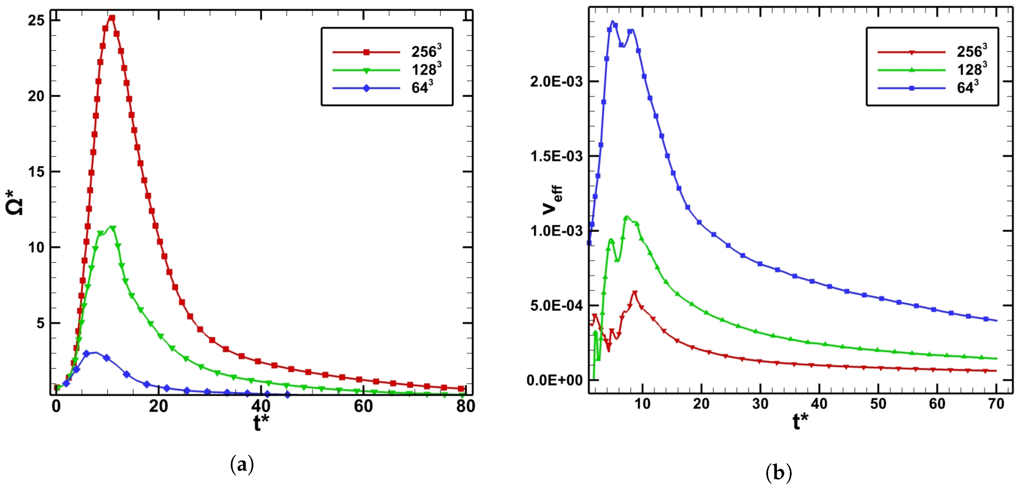
The production of vorticity is monitored for all numerical schemes and all grid levels in terms of enstrophy and effective viscosity. The latter is defined as the ratio between the kinetic energy dissipation rate and enstrophy.
Figure 5 shows the evolution of the volume average of enstrophy in time and the related development of the volumetrically-averaged effective viscosity obtained using the LES approach. DSMG-M3 results will be representative of all numerical schemes used within the ILES approach, which showed similar trends. In theory, the enstrophy should grow to infinity for an inviscid flow. Thus, this parameter is very important to study the “effective viscosity” that damps the enstrophy and stops it from growing to infinity in time. The enstrophy could be considered, in conclusion, as one of the criteria that could be used to investigate the performance and resolving power of a numerical scheme. The production of vorticity that could be observed at the early laminar stages is due to the stretching of the Taylor–Green vortex where the large-scale vorticity structures are driven towards the symmetry plane. All the numerical schemes predict a decrease in enstrophy at the stage when the flow becomes under-resolved representing the peak of the kinetic energy dissipation rate. The enstrophy decreases due to the dissipation inherent in the numerical scheme or the dissipation of the subgrid-scale model, which could be considered as an implicit or explicit numerical viscosity that is damping the production of vorticity. Using finer grid resolutions, the effective viscosity decreases, and more enstrophy could be produced. This result seems obvious since the enstrophy and effective viscosity are inversely proportional.
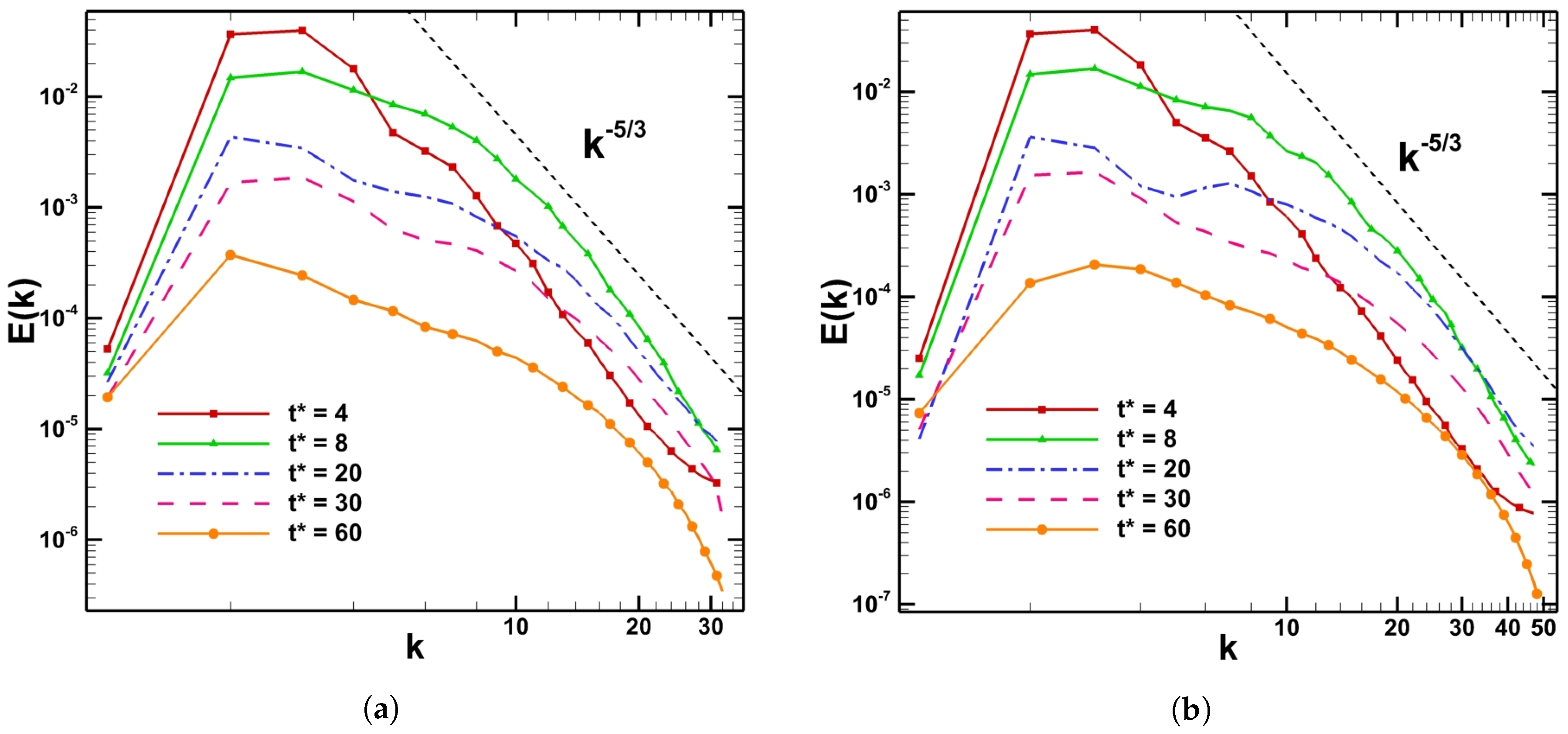
The kinetic energy spectra were monitored for all the numerical methods used in this study. The observation of kinetic energy spectra helps with understanding the flow topology and the energy cascade process.
Figure 6 presents the kinetic energy spectra obtained at different times using the M3-KK scheme on 64
and
, representing the same behaviour as the other schemes used.
A peak in the kinetic energy spectra could be observed for wavenumbers
. The same peak was observed in the study of Drikakis et al. [
29], where the authors explain that this peak in the energy spectra represents the imprint of the initial conditions used to initialize the velocity field at
. At the very early laminar stage (
), all the numerical schemes predicted a
spectrum, as has been presented in the DNS study of Brachet et al. and that corresponds to the spectrum usually found for a two-dimensional flow. This result is coherent with the fact that the three-dimensional vortex field of the TGV is initialized by a two-dimensional velocity field, and hence, the two-dimensional character of the flow is explained. As the flow becomes under-resolved, all the numerical methods including the dynamic Smagorinsky subgrid-scale model consistently emulate a
spectrum as predicted for the decaying turbulence kinetic energy spectrum. It should be noted that the dissipation of kinetic energy and the exchange of energy between the large and small scales is due to numerical dissipation inherent in the schemes being used, which acts as an implicit subgrid-scale model, and the dissipation of the explicit subgrid-scale model used in LES. The fact that all the methods succeeded in predicting the
spectrum indicates that Taylor–Green vortex flow is characterised by an inertial subrange where the small-scale vortices lose kinetic energy at the grid size level due to numerical dissipation. As the mesh is refined, the
slope becomes more accurately presented, and one could notice that at very late stages of the flow (
), the Kolmogorov scale becomes more established. It should be reminded that at this stage of TGV flow, the small-scale worm-like vortices fade-away, similarly to homogeneously-decaying turbulence.
3.3. Modified Equation Analysis
In this section, the effect of the truncation error of the second-order upwind scheme has been investigated, and the discretization of the convective term of the fully-compressible Navier–Stokes equations is carried out within the framework of the LES approach. The modified equation analysis, applied to the convective term of Navier–Stokes equations, yields the following formulation for the truncation error of the second-order upwind scheme as:
As explained earlier, the truncation error of the numerical scheme is usually neglected by most of the researchers, who claim that it has a minor effect on the accuracy of the solution, and only the numerical dissipation of the subgrid-scale model is considered. Therefore, this section aims to clarify the idea that the truncation error could have a significant contribution to the numerical dissipation of the solution. The Taylor–Green vortex helps with understanding if the subgrid-scale model dissipation is enough to predict the correct amount of kinetic energy dissipation rate or the truncation error is participating in the dissipation of kinetic energy observed during the course of the TGV simulations. For that purpose, LES performed in ANSYS-FLUENT using the dynamic Smagorinsky subgrid-scale model, second-order upwind scheme for spatial discretisation and first-order upwind scheme for temporal discretisation are considered. The truncation error derived on the right-hand side of Equation (
15) is computed using a User-Defined Function (UDF) in ANSYS-FLUENT. One could notice that the truncation error of the second-order upwind scheme has second- and third-order partial derivatives in addition to mixed partial derivatives. Only the effect of second-order partial derivatives, which are considered as the leading-order terms, is investigated in this study. It should be reminded that the second-order partial derivatives that exist in the formulation of the truncation error are present due to the fact that a first-order accurate method is used for temporal discretisation. Using higher-order temporal methods would induce third- or higher-order partial derivatives in the equation.
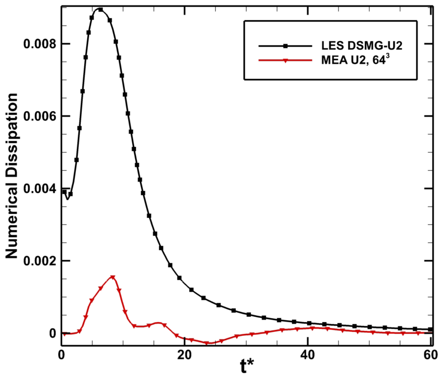
Figure 7 represents the time evolution of the leading second-order partial derivatives terms in the truncation error formulation of the second-order upwind scheme, without considering the second-order mixed partial derivatives and compared to the kinetic energy dissipation rate obtained using the dynamic Smagorinsky subgrid-scale model and second-order upwind scheme (DSMG-U2) on a 64
grid. The expression of the computed terms taken from the truncation error in Equation (
15) is:
The observed volumetrically-averaged truncation error has a time behaviour similar to the kinetic energy dissipation rate. The trend of the truncation error is characterised by an increase near
reaching a peak at about
similar to what was predicted by all the numerical schemes and the DNS study of Brachet et al. [
20,
21]. The truncation error decreases in the stages where the flow becomes disorganized. For
, negative values of truncation error could be observed, which could be due to a dispersive behaviour of the scheme since the truncation error is derived on the right-hand side in the modified Equation (
16), and hence, the negative values will be added to the left-hand side part, which induces a dispersion of the numerical solution. It is obvious from
Figure 7 that the truncation error composed of second-order partial derivatives is not negligible compared to the kinetic energy dissipation rate despite the fact that the values of the discretisation error are significantly small compared to the dissipation of kinetic energy. It should be reminded that the dissipation of kinetic energy is due to the dissipation of the subgrid-scale model and the effect of truncation error of the numerical scheme. Hence, the evolution of the kinetic energy dissipation rate represented in
Figure 7 contains both effects of the subgrid-scale model and the truncation error of the second-order upwind scheme. Therefore, if the truncation error is subtracted from the kinetic energy dissipation rate, an estimation of the subgrid-scale model dissipation could be obtained, as will be shown in
Figure 8.
The DSMG model is under-predicting the kinetic energy dissipation since its peak of dissipation is lower than the one predicted by the total dissipation of kinetic energy considering the truncation error of the upwind scheme, as well. At , dispersion in the trend of DSMG dissipation is observed due to the negative values of truncation error representing the dispersive behaviour of the scheme. the conclusion that could be drawn is that the truncation error of the numerical scheme could play a significant role in the dissipation of kinetic energy which is added to the subgrid scale model dissipation that is not giving the correct amount of numerical dissipation to model the small scales on its own. That gives motivation for researchers to reconsider their idea of always neglecting the dissipation error that is yielded by the numerical scheme being used.


