Investigation on the Relationship Between Shock Parameters and Shock Response Spectrum Under High-Magnitude Shock Environments

Abstract

The satellite–rocket separation shock environment involves transient structural responses during spacecraft release. Although its direct influence on the main structure of the satellite is limited, it can easily cause shock-sensitive precision instruments or components to fail. Nowadays, the shock response spectrum (SRS) experiment is conducted to simulate the dynamic load environment of spacecraft. There are lots of studies on the spectral pattern of SRS. Most of the existing studies focus on the qualitative effects of the shock parameters on SRS; however, quantitative relationships between key shock parameters and SRS characteristics remain relatively limited. In this study, the air cannon-based shock experiment and numerical simulation based on ANSYS/LS-DYNA 2022R1 software are conducted to investigate the influence of shock parameters on SRS. The SRS curves are fitted to quantitatively characterize their spectral features. Massive experimental and simulation datasets are systematically processed to establish the relationship between SRSs and three key shock parameters: felt thickness, bullet length, and air source pressure. A quantitative relationship based on random forest is established to map the shock parameters to the characteristics of the SRS curves. SRS curves can be calculated based on this relationship, enhancing the efficiency of SRS calculation and reducing the need for repeated SRS experiments and simulations.

1. Introduction

The optical sensing system and electronic assembly on the spacecraft are highly sensitive to high-frequency, high-g shock spectra. With the ongoing expansion of deep space exploration missions, the pyrotechnic device is widely adopted in aerospace separation mechanisms owing to its high energy density [1]. However, the transient shocks induced by actuation would damage brittle materials (e.g., crystals, ceramics) [2]. NASA’s research report shows that over 70% of launch mission failures between 1963 and 1985 are due to pyroshock damage mechanisms [3]. Thus, it is crucial to analyze such transient shock environments during spacecraft missions.

Ground experimental research is required to ensure the smooth progress of the spacecraft mission. Currently, there are four methods used to investigate spacecraft shock environments: mechanical impact method, pyrotechnic detonation method, electrodynamic shaker simulation, and laser-induced excitation method [4]. The mechanical impact method, originating from Bai and Thatcher’s metal-to-metal impact technique [5], simulates the pyroshock environment through excitation of multi-order modal resonance. The method has operational simplicity, high repeatability, and superior shock excitation capability. These features are critical to simulate the far-field environment. While the pyrotechnic detonation method provides authentic loading mechanisms and enables triaxial excitation, it introduces significant safety hazards and exhibits unacceptable result dispersion. The electrodynamic shaker simulation has the advantage of strong controllability and low cost but exhibits insufficient signal simulation capability in high-frequency regions. The laser-induced excitation method, an emerging technological method, has pronounced advantages including non-destructive operation, high energy efficiency, and environmentally friendly characteristics [6]. Notably, the excitation currently generates insufficiently high-g shock environments. It remains in the pre-engineering research phase. Hence, the mechanical impact method is widely used by many researchers.

SRS, as one of the most important research objects, can be obtained through mechanical shock experiments to describe transient shock environments in engineering practice [7,8,9]. Nowadays, there are lots of studies on investigating the SRSs under various shock conditions through the mechanical impact method. Zhao et al. [10] established a multi-parameter adjustable shock simulation platform actuated by a light gas gun. They revealed a square root dependence of SRS amplitude on air source pressure (i.e., G∝p^1/2). Based on air cannon experiments, Velmurugan et al. [11] elucidated the critical influence of composite laminate thickness on SRS and revealed that 90–95% of acceleration transfer occurs through bolted joints. Almesmari et al. [12] developed a metal-to-metal mid-field shock test facility and demonstrated that the low-frequency regions of SRS (100–1000 Hz) elevate with increasing impactor mass. By developing an adjustable air cannon device, Wang et al. [13] revealed that high-frequency amplitudes of SRSs decrease with increasing bullet density, while resonate board elastic modulus influences SRS patterns. Chen et al. [14] developed a twin-bullet air cannon shock test apparatus. The apparatus effectively addresses the issue of limited coverage associated with single-bullet configurations. Kim and Lee [15] developed an adjustable mechanical impact device. They revealed that as the thickness of resonator disk increases, the knee frequency rises, and the higher the steel ball velocity, the larger the value of SRS curve. These studies have demonstrated that different shock parameters can significantly affect the amplitude and patterns of SRS. However, most of these studies have focused on individual parameter effects or specific experimental configurations, and the quantitative mapping between multiple key shock parameters and the overall SRS patterns remains relatively limited.

Due to the low cost and convenience, numerical simulation has significantly advanced the study of shock experiments in recent years. Yalçinkaya et al. [16] conducted a shock simulation using LS-DYNA software. The results demonstrated that contact stiffness and damping coefficients significantly influence the SRS curves. Viale et al. [17] proposed an integrated parametric model incorporating a CAD modeler, finite element solver and genetic algorithm optimizer. The model can significantly reduce test calibration time and costs. Somasundaram et al. [18] investigated shock wave propagation through bolted joints under high-g shock loads using a hybrid Lagrangian–SPH modeling approach. Pi et al. [19] established a finite element model of the pyroshock simulation device using MSC.Patran software, and the influence of different hammer parameters and response plate parameters on the SRS curves is analyzed. Hu [20] established a flexible boundary particle damping honeycomb plate shock reduction method based on discrete element multibody dynamics coupling. By optimizing the relevant parameters, the peak acceleration under pyroshock was attenuated by 55.52%, thereby significantly reducing the risk of equipment failure.

To further investigate SRS, many different SRS predictive models or calculated methods have been established. Sun et al. [21] proposed a hybrid waveform synthesis method using an improved adaptive genetic algorithm (IAGA). The method resolves the high-precision synthesis challenge of pyroshock acceleration waveforms in the lack of experimental data. It significantly enhances SRS matching accuracy and practical engineering applications. A backpropagation neural network (BPNN) approach was utilized by Zhang et al. [22] to predict the shock parameters of underwater shock loading on structures, addressing the challenge of predicting complex underwater explosion effects. Zhou et al. [23] developed a probabilistic neural network (PNN) response mapping predictive method. The ground experiment data can be utilized by the method to predict the dynamic environment of aircraft in real flight conditions. Bae et al. [24] optimized the pyroshock experiment conditions for aerospace components through numerical analysis and genetic algorithms and developed an automated testing system to enhance the repeatability and reliability of the tests. Blough et al. [25] devised a method based on frequency response functions (FRF) to calculate the SRS spectral pattern. Different shock environments can be evaluated without the need for extensive experimental testing through the method. It enhances the efficiency of SRS testing and elucidates the relationships between diverse shock environments and the SRS spectral pattern. Wang et al. [26] proposed an improved method based on FRF and the virtual mode synthesis method (VMSS) for predicting the pyroshock response of spacecraft structures in a wide frequency domain. The response characteristics of spacecraft structures under pyroshock environments can be predicted more accurately by this method. These studies demonstrate the potential of numerical methods, optimization techniques, and data-driven approaches for improving shock environment prediction and reducing the dependence on repeated experiments. Nevertheless, there remains a need for an efficient quantitative model that directly maps key shock parameters to the patterns of SRS and enables rapid calculation of the SRS curve.

In this study, felt thickness, bullet length, and air source pressure are selected as three key shock parameters within the investigated parameter ranges. The purpose of establishing the quantitative relationship is not merely to describe the correlation between shock parameters and SRS, but to develop a mathematic model that can rapidly calculate SRS under different shock environments and reduce the need for repeated experiments and numerical simulations.

To establish such a quantitative relationship model, systematic research on the relationship is conducted in this paper. Firstly, mechanical shock experiments are carried out using an air cannon device, with variations in parameters including felt thickness, bullet length, and air source pressure. LS-DYNA explicit dynamics simulation software is used to simulate the shock environment. The simulated SRSs show good agreement with the experimental SRSs. Based on both the experimental and simulation results, the effects of these shock parameters on the SRSs are analyzed. Furthermore, the experimental and simulated SRS curves are accurately fitted by MATLAB R2023b, and the relationship between the coefficients of the fitting equation and the shock parameters is studied based on the random forest machine learning algorithm. Finally, the SRS quantitative relationship is established. The accuracy of the relationship model is rigorously validated through multiple experiments. The results demonstrate that the proposed model can provide an efficient method of calculating SRS curves within the investigated parameter ranges, thereby providing a basis for preliminary shock environment evaluation.

2. Simulator of Pyroshock Environment

2.1. Experimental Setup

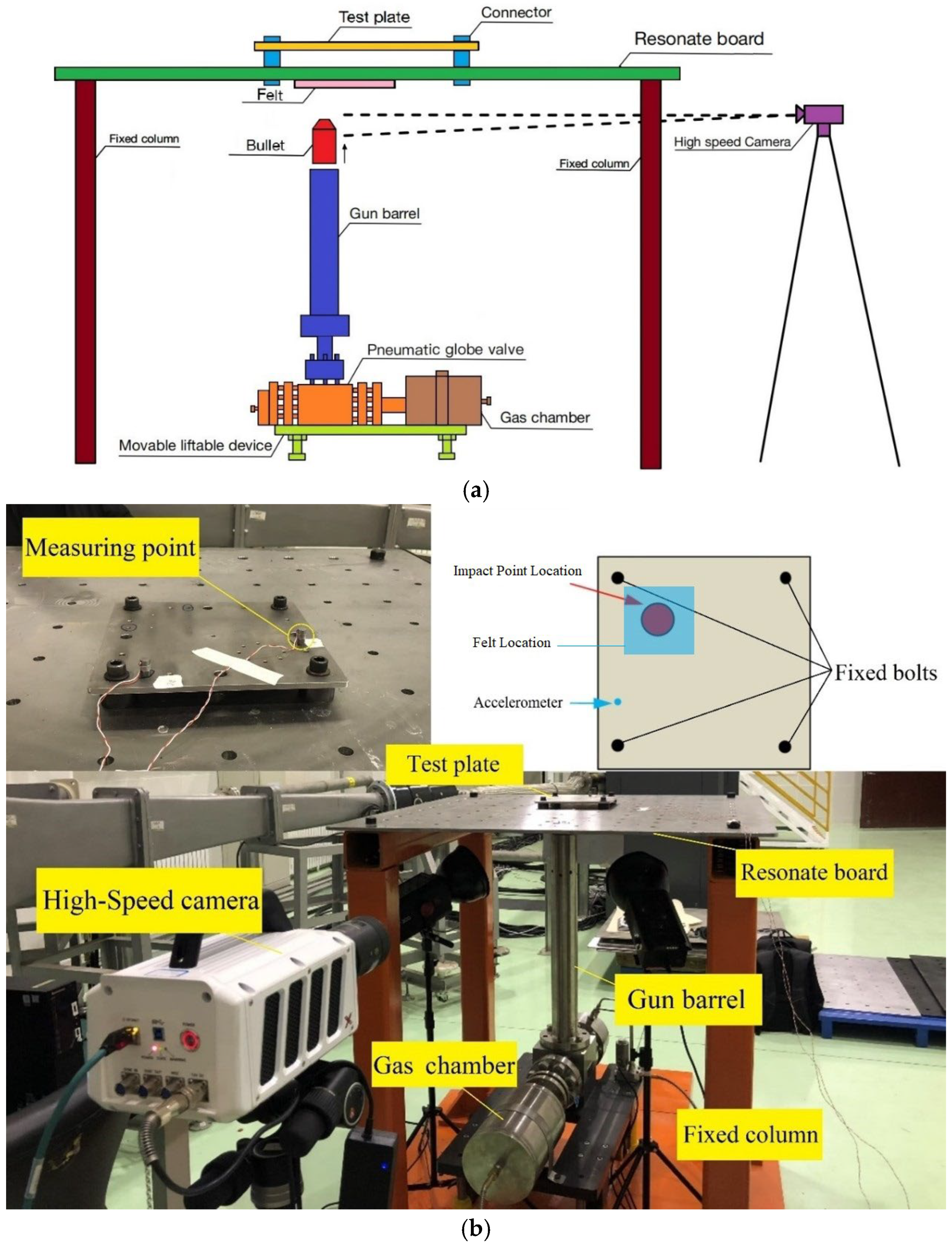
Figure 1a,b show the schematic and physical diagrams of the air cannon device, respectively. The air cannon device is composed of a pneumatic globe valve, gas chamber, gun barrel and movable liftable device. The fixed columns connect the resonate board to the ground, maintaining the equipment in a horizontal position. The air cannon device is situated directly beneath the resonate board. To achieve automatic adjustment and precise control of the air cannon pressure, an automatic pressure regulator and a pressure transmitter are employed. High pressure is generated in the gas chamber to propel the bullet so that it impacts the resonate board perpendicularly at high speed, thereby achieving shock environment loading. After impacting the resonate board, the bullet bounces back to the interior of the gun barrel, protecting the test device and testing workers. To obtain the bullet shock velocity, a high-speed camera is employed to capture the collision between the bullet and the resonate board, while the accelerometer is used to measure the acceleration signal during impact.

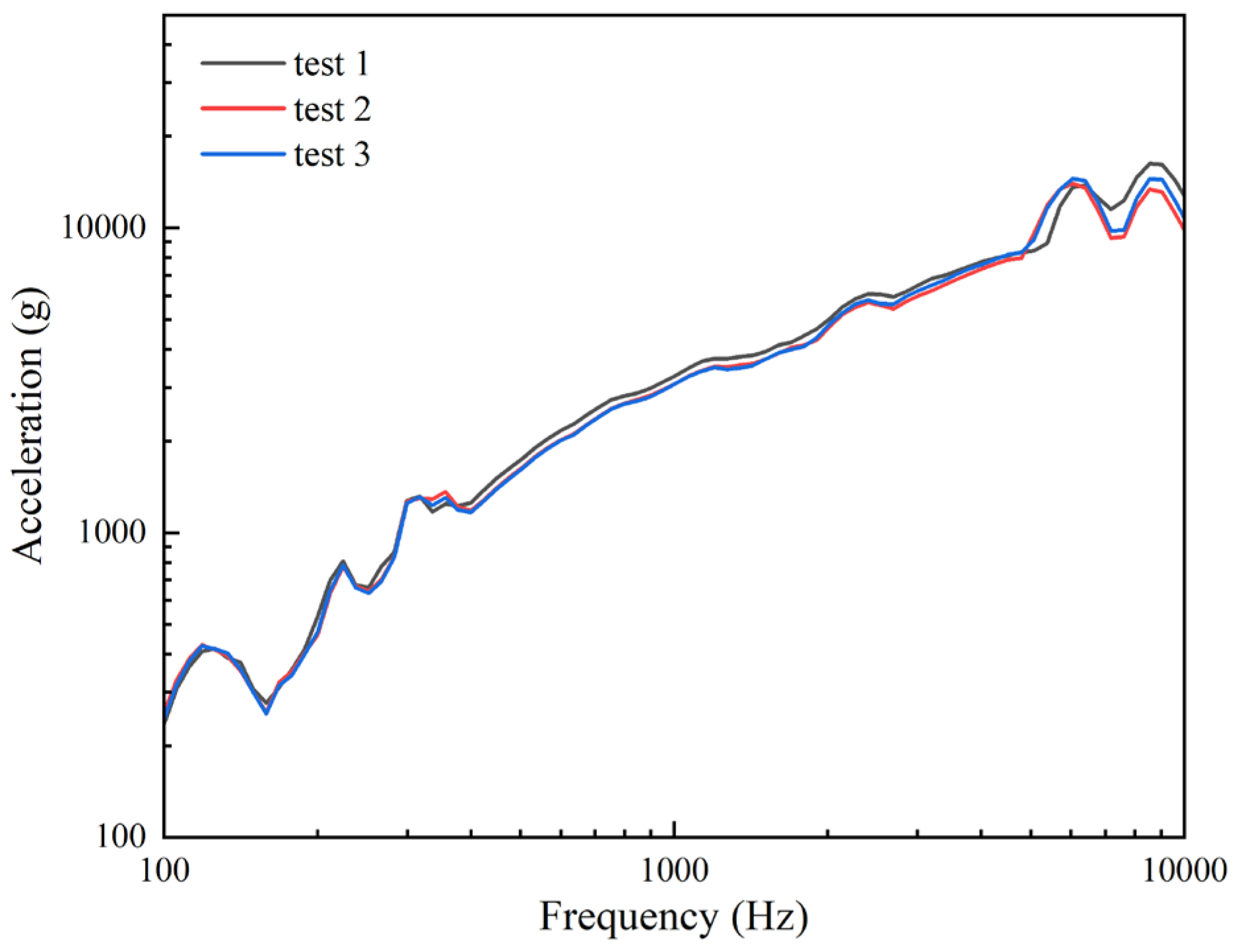
Good consistency is the prerequisite for high reliability of experimental results. Thus, three repeated shock tests are carried out with the air cannon device before the formal experiments. Figure 2 displays the SRSs in the three shock tests. It can be seen from the figure that the three SRS curves are essentially in close proximity to one another. The results indicate that the SRSs maintain high consistency under an identical shock environment.

In this study, three critical experimental parameters are systematically varied to investigate the effects of shock environments on SRSs: felt thickness (0 mm, 5 mm, 10 mm, 15 mm), air source pressure (0.5 MPa, 0.7 MPa, 0.9 MPa), and bullet length (70 mm, 120 mm, 200 mm). Preliminary experiments and numerical simulations were also conducted for other potential parameters, such as bullet impact location, specimen area, accelerometer location and bolt connection type. The results indicated that their effects on the SRS were less pronounced than those of the three selected parameters. Therefore, this study focuses on these three key parameters, which exhibited relatively more pronounced effects on the SRS.

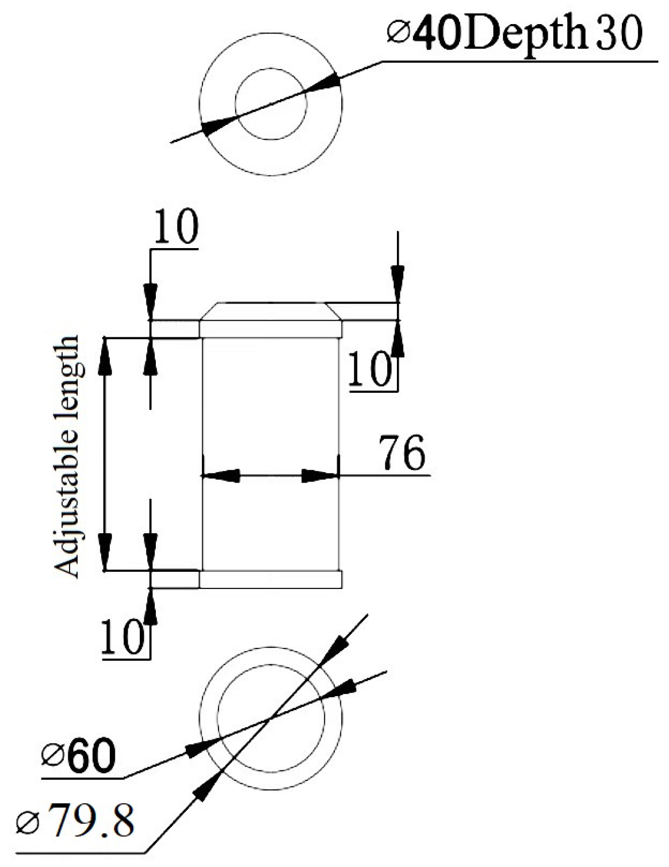
A total of 36 experiments were conducted by varying these three parameters. The resonate board, test device, and bullet are all made of steel. The resonate board has dimensions of 1200 mm × 1200 mm × 10 mm, the test device has dimensions of 250 mm × 250 mm × 15 mm, and the size of the bullet is as shown in Figure 3. The felt is 150 mm × 150 mm with adjustable thickness, which is made of industrial felt.

2.2. Finite Element Analysis

The shock environment has typical transient characteristics; the ANSYS/LS-DYNA 2022R1 software is selected for analysis. The Lagrange method is the primary solution method in LS-DYNA because it has strong explicit dynamics analysis capabilities and can simulate a variety of complex structural shock situations. Thus, it can satisfy the solution of the shock environment.

The simulation model comprises three components: the bullet, the resonate board, and the test plate. The influences of a few tiny chamfers and threaded holes are disregarded throughout the modeling phase. To prevent initial contact, there is a gap between the bullet and the resonate board. The speed value of the bullet can be obtained by the high-speed camera. The velocity direction of the bullet is perpendicular to the resonate board. The resonate board is fixed at four points to mimic its real-world constraints. Additionally, there are no initial displacements, stresses, or strains.

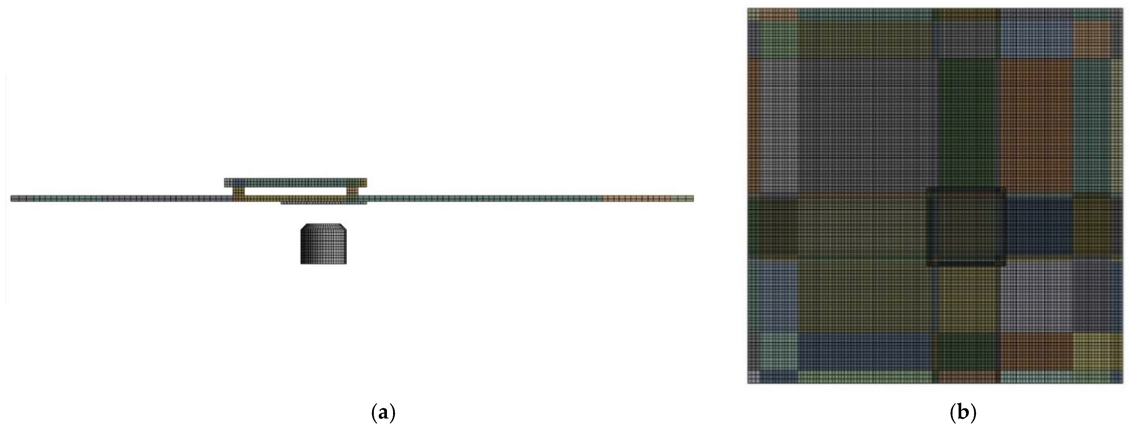
During the finite element computation, the mesh distortion is prone to occur, leading to significant deviations in the calculation results. To ensure the accuracy of the calculation results, the entire model is meshed using SOLID164 hexahedral elements. Due to the intense shock generated by the bullet, the shock wave exhibits transient, high-frequency and high-amplitude characteristics. To more accurately capture the propagation and response of the impact, local mesh refinement is applied to the critical region surrounding the impact point. The finite element model is shown in Figure 4.

To improve the accuracy of the simulated SRS, the response data are extracted from several nodes located at the accelerometer installation sites. These nodal values are then averaged to reduce error.

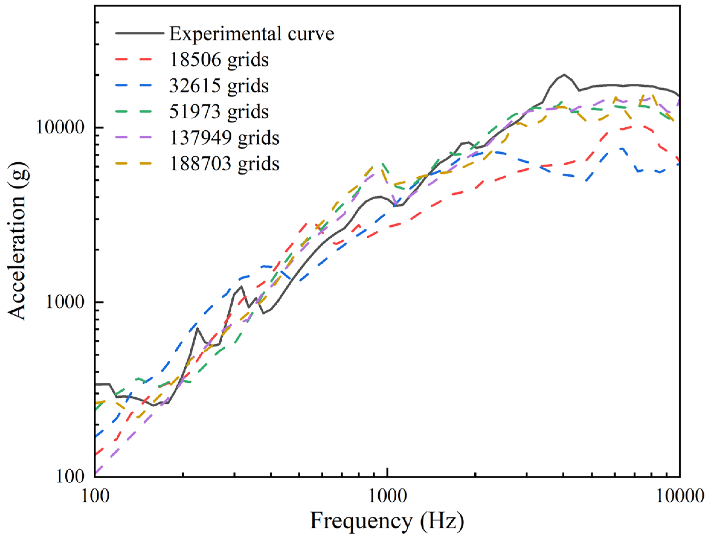
In finite element analysis, the sparsity of the grid has a significant influence on the accuracy of the calculation results. To strike a balance between computational accuracy, time and space, the grid independence verification is conducted. The models with grid numbers 18506, 32615, 51973, 137949 and 188703 are computed, and the SRSs are obtained, as shown in Figure 5. It can be seen from the figure that the simulated SRSs computed on the 18506-element grid and the 32615-element grid markedly deviate from the experimental SRS. The simulated SRS computed on the 51973-element grid is essentially consistent with the experimental SRS. Further grid refinement beyond 51973 elements shows negligible influence on results. Therefore, a grid count of 51973 is the most reasonable choice. All numerical simulations in this study are conducted by this meshing approach.

3. Pyroshock Environmental Parameters and Law Research

3.1. Effect of Felt Thickness

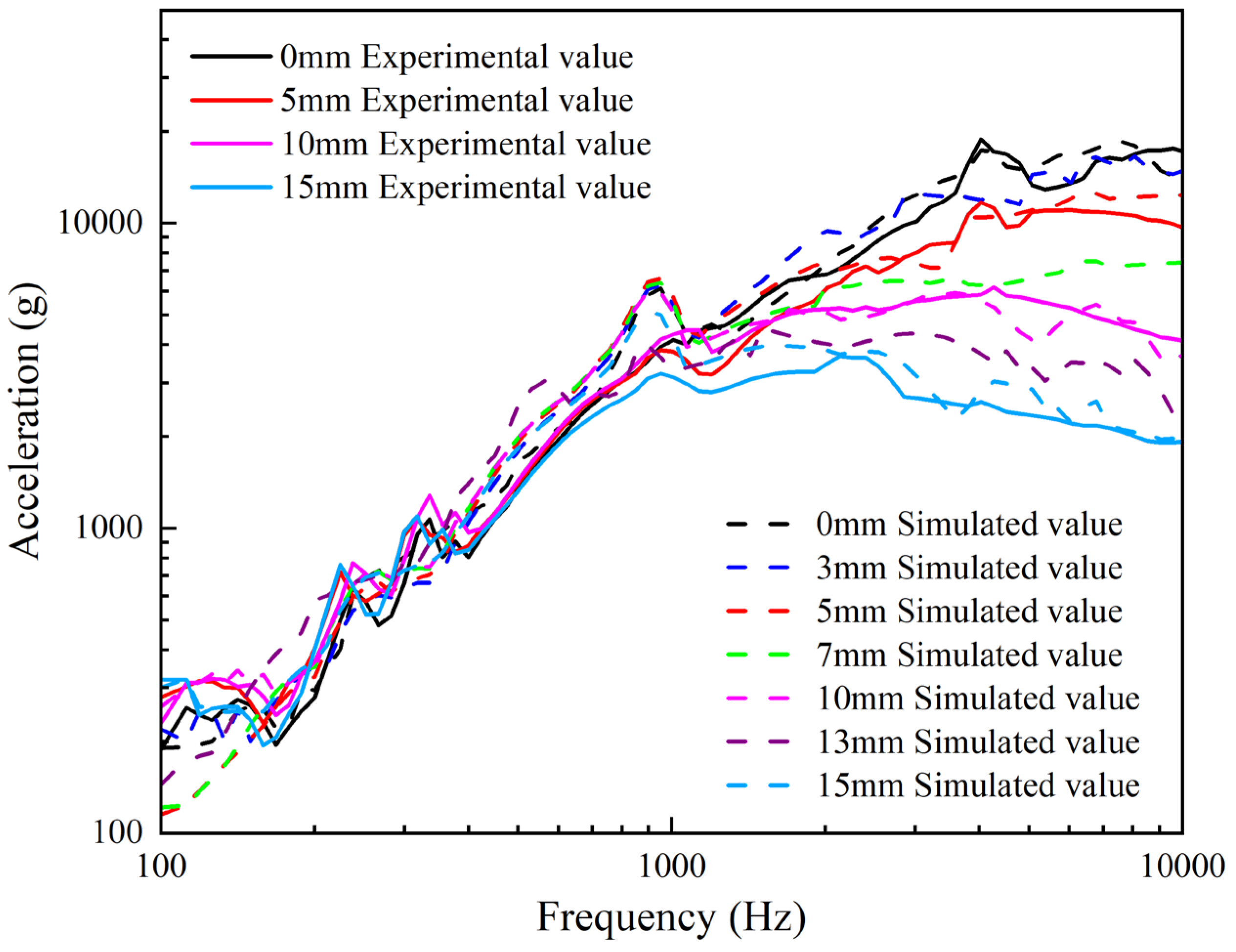
To investigate the effect of felt thickness on SRS, experiments and numerical simulations are conducted under various felt thickness conditions. Figure 6 shows the SRS curves under different felt thicknesses. These SRS curves are generated using a 70 mm bullet under 0.5 MPa. When there is no felt, the experimental SRS is shown by the black solid line in the figure. The SRS knee frequency is at approximately 5000 Hz. The low-frequency slope is 7.11 dB/oct. Additionally, experiments are conducted under conditions where the felt thicknesses are 5 mm, 10 mm, and 15 mm. With the increase in felt thickness, the SRS knee frequency decreases progressively: from 5000 Hz (D = 0 mm) to 4000 Hz (D = 5 mm), then to 3000 Hz (D = 10 mm), and finally to 1000 Hz (D = 15 mm). Meanwhile, the low-frequency slope remains approximately constant at around 7 dB/oct. These results indicate that the increase in felt thickness has a noticeable influence on the knee frequency but a negligible influence on the low-frequency slope. Subsequently, SRSs are simulated under conditions of 0 mm, 5 mm, 10 mm, and 15 mm felt thickness, with the results shown as dashed lines in Figure 6. The experimental and simulated SRSs exhibit a high degree of agreement. To quantify the deviation between simulated and experimental values, the Mean Absolute Logarithmic Error (MALE) is introduced as the evaluation metric in this study, whose mathematical expression is written as Equation (1):

$$\mathrm{MALE}={\displaystyle \frac{1}{N}}{\displaystyle \sum _{i=1}^N\left|\lg \left(\frac{y_i^{sim}}{y_i^{exp}}\right)\right|}$$

(1)

where N represents the number of points on the SRS curve, and $y_i^{sim}$ and $y_i^{exp}$ are the simulated value and experimental value at the i-th point, respectively. The mean absolute value of the logarithmic ratio between simulated and experimental values is calculated by the equation, effectively characterizing the distribution features of relative errors in logarithmic coordinates.

The MALE values for the felt thicknesses are: 6.32% (D = 0 mm), 9.45% (D = 5 mm), 5.77% (D = 10 mm), and 7.71% (D = 15 mm). All MALE values are less than 10%, indicating that the simulated values are in good agreement with the experimental values. To further study the effect of felt thickness on SRSs, numerical simulations are conducted with felt thicknesses of 3 mm, 7 mm, and 13 mm. The simulated results show that the increase in felt thickness progressively decreases high-frequency amplitude, while the low-frequency slope remains largely unchanged. The knee frequency gradually decreases with increasing felt thickness. This phenomenon can be attributed to the viscoelasticity of felt. The felt absorbs energy due to the deformation of felt during the process of bullet impact, thereby reducing the force transmitted to the resonate board [10]. When there is no felt, the impact force generated by the bullet transfers rapidly to the resonate board. The high-frequency amplitude of the SRS primarily characterizes the system response to the instantaneous and rapidly varying components of the shock, typically associated with intense transient vibrations [13]. The rapid energy transfer induces high-magnitude vibrations, generating prominent high-frequency components in the SRS. With increasing felt thickness, the energy dissipation capacity is enhanced, and the impact force transmitted to the resonate board is attenuated. Consequently, the transient vibration of the resonate board is suppressed, leading to progressive reduction in high-frequency components in the SRS. At the same time, the felt serves as the primary contributor to the equivalent stiffness (k) of the system. The increase in felt thickness can reduce the equivalent stiffness. According to the relationship between natural frequency (f_n) and equivalent stiffness (i.e., f_n ∝ k^1/2) [27], the reduction in the equivalent stiffness of the system causes a decrease in the natural frequency. The knee frequency is typically strongly correlated with the natural frequency of the system [15,28]. As felt thickness increases, the reduction in system equivalent stiffness and natural frequency causes the SRS knee frequency to shift toward lower frequencies.

3.2. Effect of Air Source Pressure

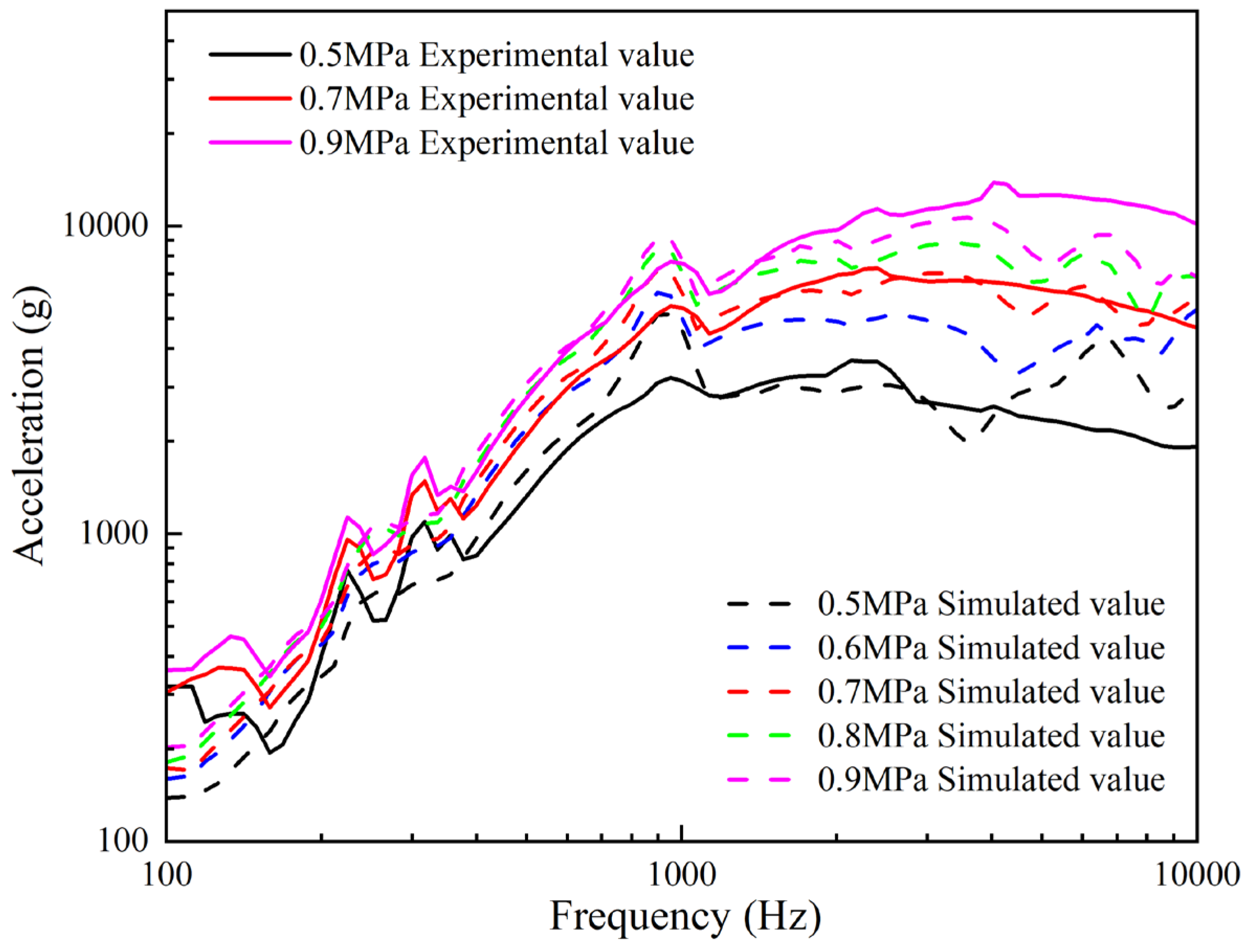
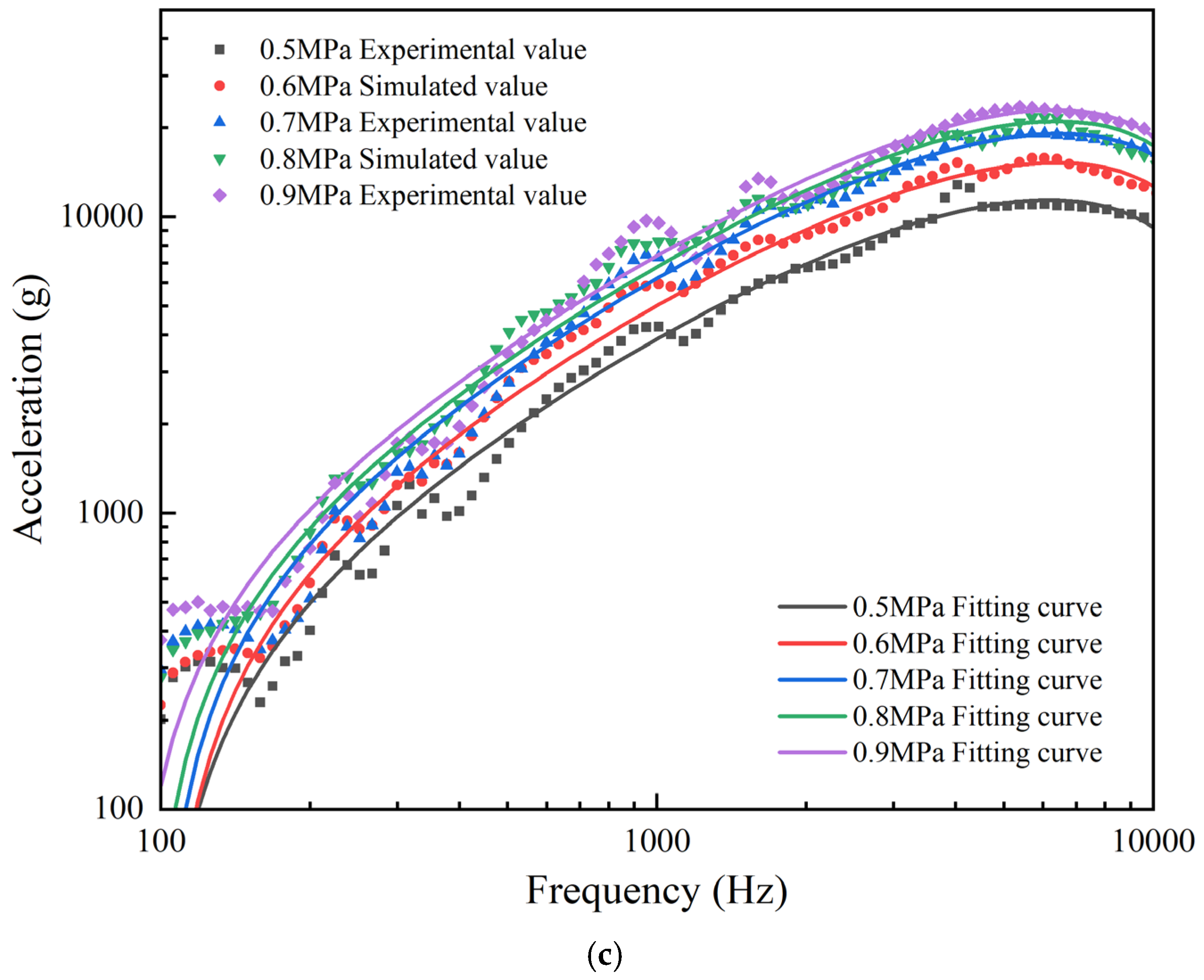
Figure 7 shows the SRS curves under different air source pressures. The bullet length is 70 mm, and the felt thickness is 15 mm in the experiment. At the air source pressure of 0.5 MPa, the SRS knee frequency occurs at approximately 1000 Hz. The low-frequency slope measures 7.39 dB/oct. Beyond the knee frequency, the acceleration values remain essentially stable within the high-frequency region, as indicated by the solid black line in Figure 7. Subsequently, experiments are conducted under air source pressures of 0.7 MPa and 0.9 MPa. It can be observed that with the increase in air source pressure, the knee frequencies remain around 1000 Hz, while the low-frequency slopes are at approximately 7.3 dB/oct. However, as the air source pressure increases, the peak acceleration at the knee frequency rises from 3128.4 g (P = 0.5 MPa) to 5403.0 g (P = 0.7 MPa) and further increases to about 7552.2 g (P = 0.9 MPa). The results show that the air source pressure primarily influences the amplitude of the SRSs while exhibiting negligible effects on its spectral pattern. Then, SRSs are simulated under pressures of 0.5 MPa, 0.7 MPa, and 0.9 MPa, with the results shown as dashed lines in Figure 7. The MALE values for the air source pressures are: 9.71% (P = 0.5 MPa), 6.94% (P = 0.7 MPa), 9.31% (P = 0.9 MPa). All MALE values are less than 10%, indicating that the simulated values are in good agreement with the experimental values. To investigate the influence of air source pressure on SRS, numerical simulations are conducted under air source pressures of 0.6 MPa and 0.8 MPa. It shows that the spectral patterns of the SRSs remain essentially consistent under different pressures, and with increasing air source pressure, the overall amplitude of the SRS increases. This is because the bullet velocity exhibits a square root relationship with the air source pressure (i.e., v ∝ p^1/2) [10]. The higher air source pressure can generate greater bullet velocity, consequently increasing the kinetic energy of bullet. Thus, the increase in kinetic energy generates stronger acceleration inputs to the resonate board, thereby elevating SRS amplitudes.

3.3. Effect of Bullet Length

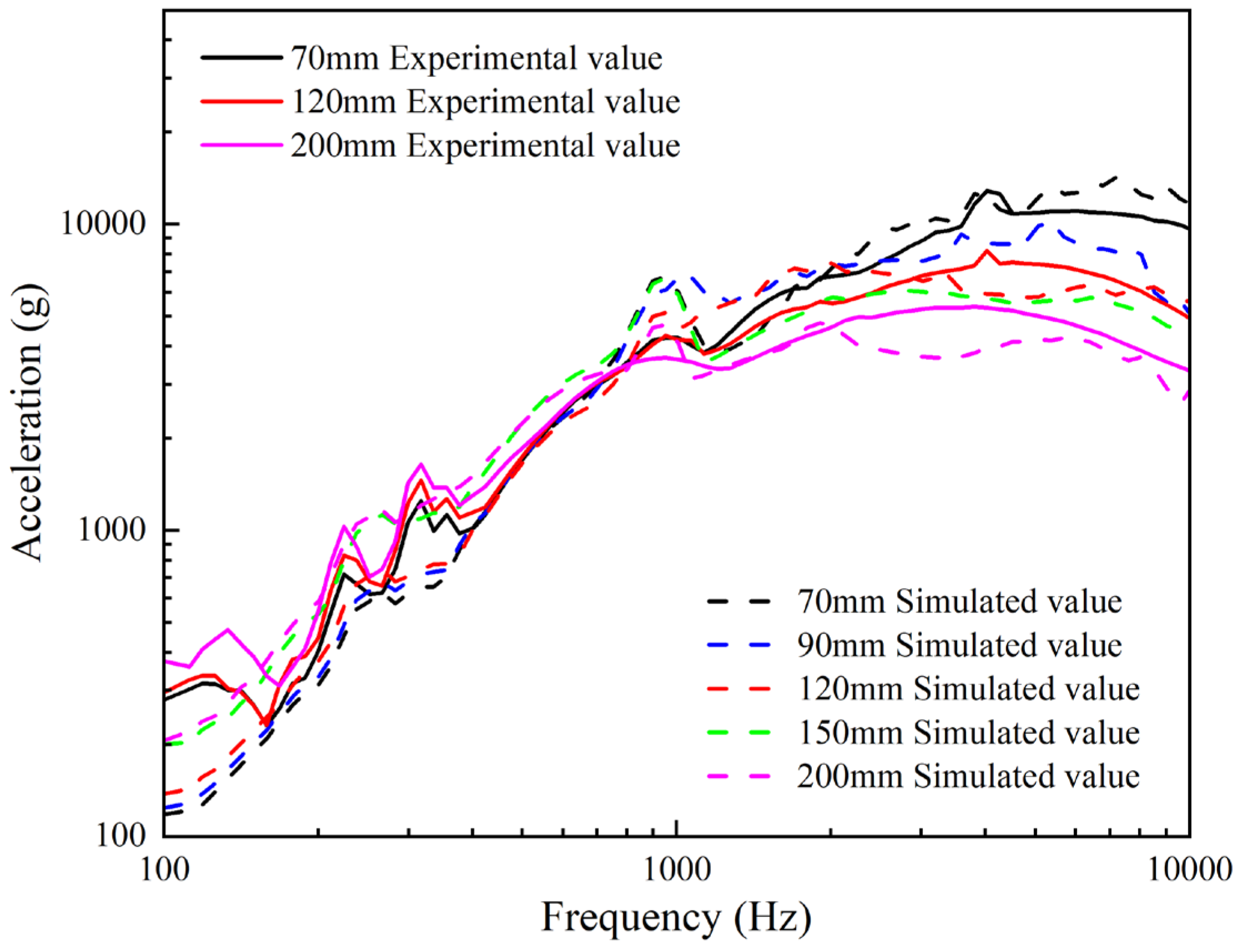
Figure 8 shows the SRS curves under different bullet lengths. These SRS curves are generated using a 5 mm felt under 0.5 MPa. Under the condition of using a 70 mm bullet, the SRS curve shows a knee frequency at approximately 4000 Hz. The low-frequency slope is 7.10 dB/oct. Beyond the knee frequency, the response remains stable within the high-frequency region, as indicated by the solid black line in Figure 8. Subsequently, experiments are conducted with bullets of 120 mm and 200 mm length. The experimental SRSs reveal that increasing bullet length progressively elevates the response levels of SRSs within the 100–1000 Hz range, whereas it gradually decreases the SRS amplitudes in the 1000–10,000 Hz region. The knee frequencies are all around 4000 Hz. For the 120 mm and 200 mm bullets, the low-frequency slopes are 6.90 dB/oct and 5.91 dB/oct, respectively. The results demonstrate that a change in bullet length will lead to a change in both the low-frequency slope and high-frequency amplitude of SRSs. Then, simulated SRSs at bullet lengths of 70, 120, and 200 mm are presented as dashed curves in Figure 8. The MALE values for the bullet lengths are: 9.49% (h = 70 mm), 9.41% (h = 120 mm), 8.39% (h = 200 mm). All MALE values are less than 10%, indicating that the simulated values show good agreement with the experimental values. To investigate bullet length effects on SRS, numerical simulations are conducted for 90 mm and 150 mm. It shows that increasing bullet length reduces both the low-frequency slope and high-frequency amplitudes of the SRS. This phenomenon may stem from the fact that a longer bullet amplifies input force and extends impact duration, thereby elevating impulse transfer. The change in impulse transfer affects the response of the resonate board, causing the low-frequency region of the SRS to rise. Additionally, with the increase in bullet length, the bullet mass increases while the shock velocity decreases. The reduction in velocity will suppress excitation of high-frequency modes. Consequently, SRS amplitudes in the high-frequency region attenuate.

4. Quantitative Relationship Between SRS and Shock Parameters

4.1. Random Forest Algorithm

Random forest is a typical ensemble machine learning algorithm derived from the bagging framework. It enhances model generalization performance by constructing and integrating a set of independent decision trees. It adopts a dual random mechanism, including bootstrap resampling to generate independent training subsets and random feature subspace selection during node splitting. This strategy reduces the correlation among individual decision trees and mitigates the risk of overfitting.

Integrated aggregation of multiple decision trees serves as the core mechanism of this algorithm. For regression tasks, the final calculation value is obtained by averaging the outputs of all decision trees, as shown in Equation (2):

$$\widehat{y}={\displaystyle \frac{1}{B}}{\displaystyle \sum _{b=1}^B{T}_b\left(x\right)}$$

(2)

where B represents the number of decision trees, T_b(x) denotes the calculation result of a single decision tree, and $\widehat{y}$ is the calculation value of the model.

4.2. Establishment of Quantitative Relationship

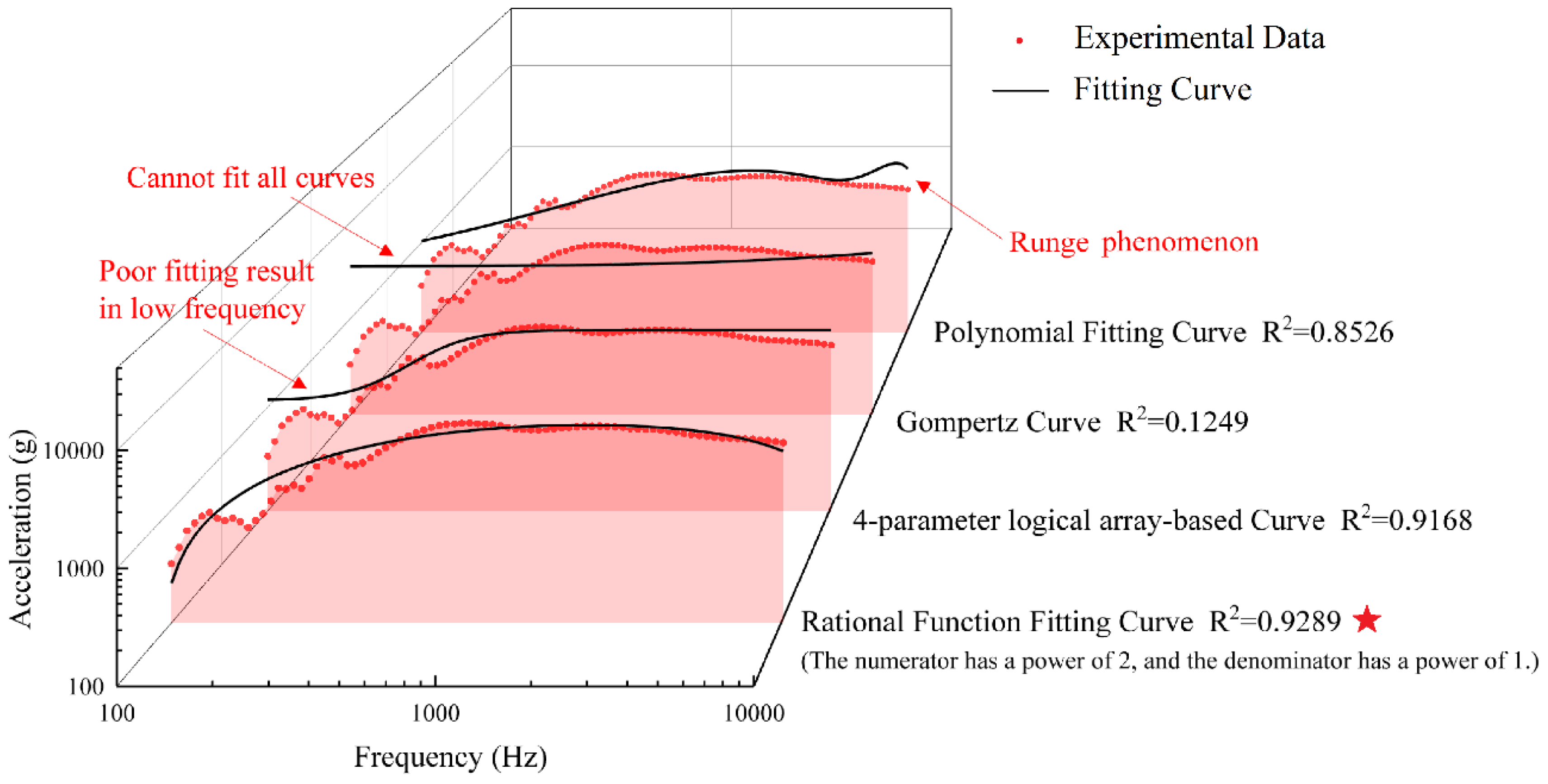
In order to investigate the spectral pattern of SRS quantitatively, it is necessary to find the appropriate fitting curve of the experimental and simulated SRSs. Different curve equations are used to fit the SRSs, such as the four-parameter logical array-based curve, Gompertz curve, polynomial fitting curve and rational function fitting curve (the numerator has a power of 2, and the denominator has a power of 1).

Table 1. Mathematical expressions of different curve equations.

Curve Name	Curve Equation
4-Parameter Logical Array-Based Curve	$f\left(x\right)=a+{\displaystyle \frac{b}{{\left(1+\raisebox{1ex}{$x$}\!\left/ \!\raisebox{-1ex}{$c$}\right.\right)}^d}}$
Gompertz Curve	$f\left(x\right)=a+b{e}^{-e^{c\left(x-d\right)}}$
Polynomial Fitting Curve	$f(x)=a{x}^4+b{x}^3+c{x}^2+dx+e$
Rational Function Fitting Curve *	$f\left(x\right)={\displaystyle \frac{p_1{x}^2+p_{2}x+p_3}{x+q_1}}$

* Levenberg–Marquardt algorithm is adopted for fitting.

shows the mathematical expressions of the curve equations.

To quantitatively assess the goodness-of-fit for the curve, the coefficient of determination (R²) is employed as the evaluation metric. The mathematical formulation of this metric is presented in Equation (3). The fitting results of different equations for the SRS under identical shock environments are shown in Figure 9.

$${\mathrm{R}}^2=1-{\displaystyle \frac{{\displaystyle \sum _{i=1}^n{\left({\widehat{y}}_i-y_i\right)}^2}}{{\displaystyle \sum _{i=1}^n{\left({\widehat{y}}_i-\overline{y}\right)}^2}}}$$

(3)

where ${\widehat{y}}_i$ is the fitted value at the i-th frequency;${ y}_i$ is the experimental value at the i-th frequency;$\overline{y}$ is the mean of the experimental value.

By comparison, the four-parameter logical array-based curve exhibits poor fitting result in the low-frequency region. The Gompertz curve shows poor fitting results in both the low- and high-frequency regions. When the polynomial fitting is employed, low-order polynomials (first to third order) cannot effectively characterize the SRSs, resulting in poor fitting results. However, while increasing the polynomial order improves the fitting result, it also introduces new problems: higher-order polynomials are prone to producing Runge’s phenomenon at higher frequencies, causing significant deviations in the fitting curve. In contrast, the rational function fitting curve with a numerator order of 2 and a denominator order of 1 demonstrates optimal spectral approximation capability. It has superior fitting results in both the low- and high-frequency regions. For the purpose of further investigating the applicability of the fitting equations, SRS curves under various conditions are fitted using these equations. The rational function fitting demonstrates high adaptability and achieves good fitting results. The four-parameter logical array-based curve demonstrates inferior adaptability and generates less favorable fitting results compared to rational function fitting. The Gompertz curve fitting is relatively poor, and most SRSs cannot be well fitted. The higher-order polynomial fitting tends to produce ill-conditioned equations, resulting in deteriorated condition numbers. Consequently, this phenomenon induces numerical instability, thereby making it impossible to accurately characterize the SRS curves.

In summary, the rational function fitting is selected to characterize SRSs. The curve equations in

Table 2. Fitting equations for different felt thicknesses (P = 0.5 MPa, h = 70 mm).

Felt Thickness (D) (mm)	Fitting Equation	R2 Value
0	$g={\displaystyle \frac{-4.5213f^2+9.2015\times {10}^{4}f-7.6654\times {10}^6}{f+1.7623\times {10}^4}}$	0.9521
3	$g={\displaystyle \frac{-3.4087f^2+6.5029\times {10}^{4}f-5.7326\times {10}^6}{f+1.2456\times {10}^4}}$	0.9640
5	$g={\displaystyle \frac{-2.8352f^2+4.6432\times {10}^{4}f-4.5667\times {10}^6}{f+9.0878\times {10}^3}}$	0.9864
7	$g={\displaystyle \frac{-1.5723f^2+2.3555\times {10}^{4}f-2.9803\times {10}^6}{f+3.6942\times {10}^3}}$	0.8440
10	$g={\displaystyle \frac{-0.6289f^2+1.0481\times {10}^{4}f-1.2900\times {10}^6}{f+1.3184\times {10}^3}}$	0.9789
13	$g={\displaystyle \frac{-0.4012f^2+6.8970\times {10}^{3}f-8.6981\times {10}^5}{f+700.8000}}$	0.9496
15	$g={\displaystyle \frac{-0.3455f^2+5.1460\times {10}^{3}f-6.2277\times {10}^5}{f+456.8850}}$	0.8944

,

Table 3. Fitting equations for different bullet lengths (P = 0.5 MPa, D = 5 mm).

Bullet Length (h) (mm)	Fitting Equation	R2 Value
70	$g={\displaystyle \frac{-2.8352f^2+4.6432\times {10}^{4}f-4.5667\times {10}^6}{f+9.0878\times {10}^3}}$	0.9864
90	$g={\displaystyle \frac{-1.8493f^2+3.0695\times {10}^{4}f-2.6717\times {10}^6}{f+4.8282\times {10}^3}}$	0.9541
120	$g={\displaystyle \frac{-1.1419f^2+1.7932\times {10}^{4}f-1.5657\times {10}^6}{f+2.5556\times {10}^3}}$	0.9193
150	$g={\displaystyle \frac{-0.7747f^2+1.3386\times {10}^{4}f-1.1190\times {10}^6}{f+1.7153\times {10}^3}}$	0.9242
200	$g={\displaystyle \frac{-0.4633f^2+9.9193\times {10}^{3}f-8.1366\times {10}^5}{f+1.1863\times {10}^3}}$	0.9278

and

Table 4. Fitting equations for air source pressures (D = 5 mm, h = 70 mm).

Air Source Pressure (P) (MPa)	Fitting Equation	R2 Value
0.5	$g={\displaystyle \frac{-2.8352f^2+4.6432\times {10}^{4}f-4.5667\times {10}^6}{f+9.0878\times {10}^3}}$	0.9864
0.6	$g={\displaystyle \frac{-3.6209f^2+6.2695\times {10}^{4}f-6.3309\times {10}^6}{f+9.1651\times {10}^3}}$	0.9913
0.7	$g={\displaystyle \frac{-4.5893f^2+7.8595\times {10}^{4}f-7.7865\times {10}^6}{f+9.6789\times {10}^3}}$	0.9926
0.8	$g={\displaystyle \frac{-5.7401f^2+9.5949\times {10}^{4}f-8.9351\times {10}^6}{f+1.0627\times {10}^4}}$	0.9896
0.9	$g={\displaystyle \frac{-7.0735f^2+1.1294\times {10}^{5}f-9.7746\times {10}^6}{f+1.2012\times {10}^4}}$	0.9869

are obtained by the rational function fitting. They present the fitting equations for varying felt thickness, bullet length, and air source pressure, respectively. It can be seen from the tables that all the R² values are above 0.8, which demonstrates that the SRS curves can be highly fitted by the rational function fitting curve.

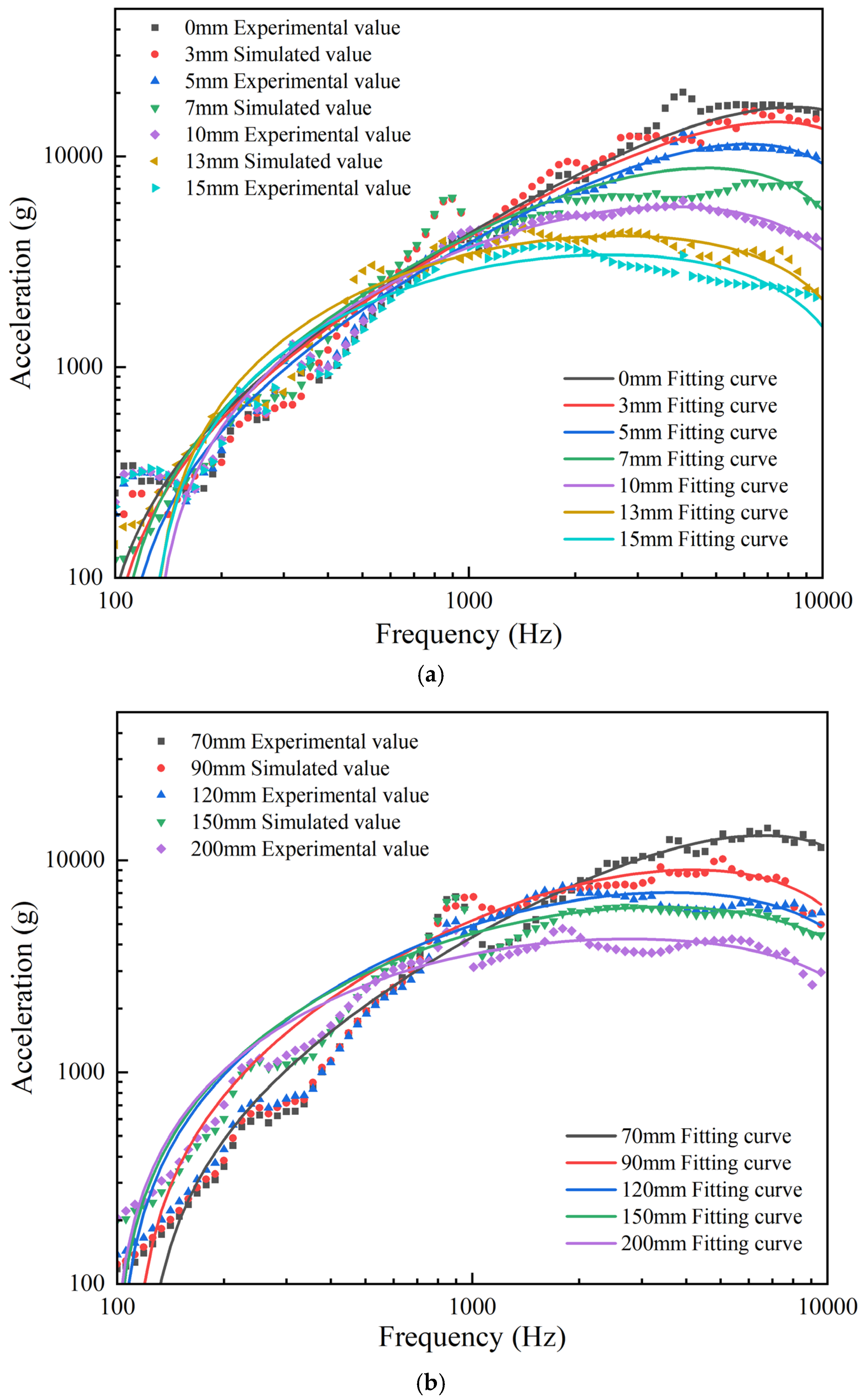
The SRS fitting curves under different conditions based on the rational function equation are shown in Figure 10. In Figure 10, the points of different colors represent the experimental or simulated SRS data under different shock environments, while the curves of different colors represent the fitting curves for each shock environment. It can be seen that the fitting curves and the SRS curves are well fitted. As the felt thickness increases, the fitting curve gradually decreases at high frequencies while remaining essentially unchanged at low frequencies. With the increase in bullet length, the fitting curve gradually increases at low frequencies while gradually decreasing at high frequencies. As the air source pressure increases, the fitting curve shifts upward as a whole. This rule is consistent with the description in the previous section.

It is essential to establish a mapping relationship between the shock parameters—felt thickness, air source pressure, and bullet height—and the equation coefficients p₁, p₂, p₃, q₁. In view of the high-dimensional and nonlinear characteristics of the mapping, the random forest (RF) algorithm is employed to find the relationship. The RF algorithm has significant advantages in dealing with high-dimensional data and complex nonlinear relationships to ensure the accuracy and stability of calculation results. In addition, the RF algorithm is adaptive in feature selection, which can effectively reduce the overfitting phenomenon and improve the generalization ability, so that it can make full use of the information in the experimental data and have high computational efficiency. It can be seen from Table 1, Table 2 and Table 3 that as the felt thickness, bullet height, and air source pressure change, the equation coefficients p₁, p₂, p₃, and q₁ exhibit significant variations. Specifically, as the felt thickness and bullet length increases, the absolute values of p₁, p₂, p₃, q₁ gradually decrease. Conversely, the increase in air source pressure results in a gradual increase in these coefficients. The relationship demonstrates that there is a good correlation between the input variables (D, P, h) and the target variables (p₁, p₂, p₃, q₁). Based on the relationship, the corresponding mathematical expression can be established, as shown in Equation (4).

$$Y=f\left(X\right)$$

(4)

where X = [P, D, h] represents the vector of the input variables; Y = [p₁, p₂, p₃, q₁] represents the vector of the target variables; f (·) represents the function mapping between the input and the target variable. Through Equation (3), the parameters p₁, p₂, p₃, and q₁ can be calculated under given shock conditions, thereby enabling the construction of the SRS curve.

The selected 100 datasets in this study contain no outliers and do not need to be preprocessed. To mitigate interference caused by the results during data analysis, the min–max normalization is applied to standardize the data. Specifically, 80% of the data (80 samples) are allocated as the training set, while the remaining 20% (20 samples) serve as the testing set. The standardized data are imported into MATLAB, and RF algorithm is implemented for training.

4.3. Validation of Quantitative Relationship

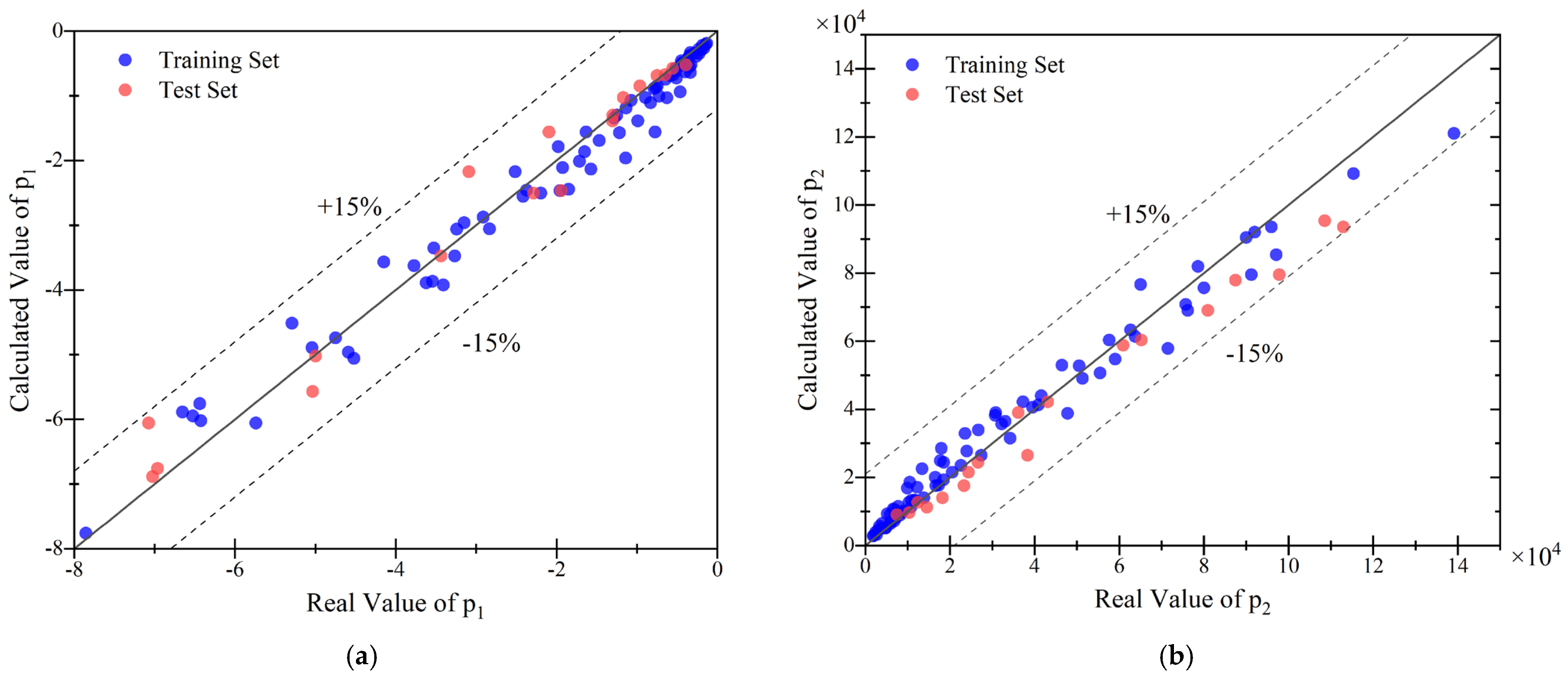
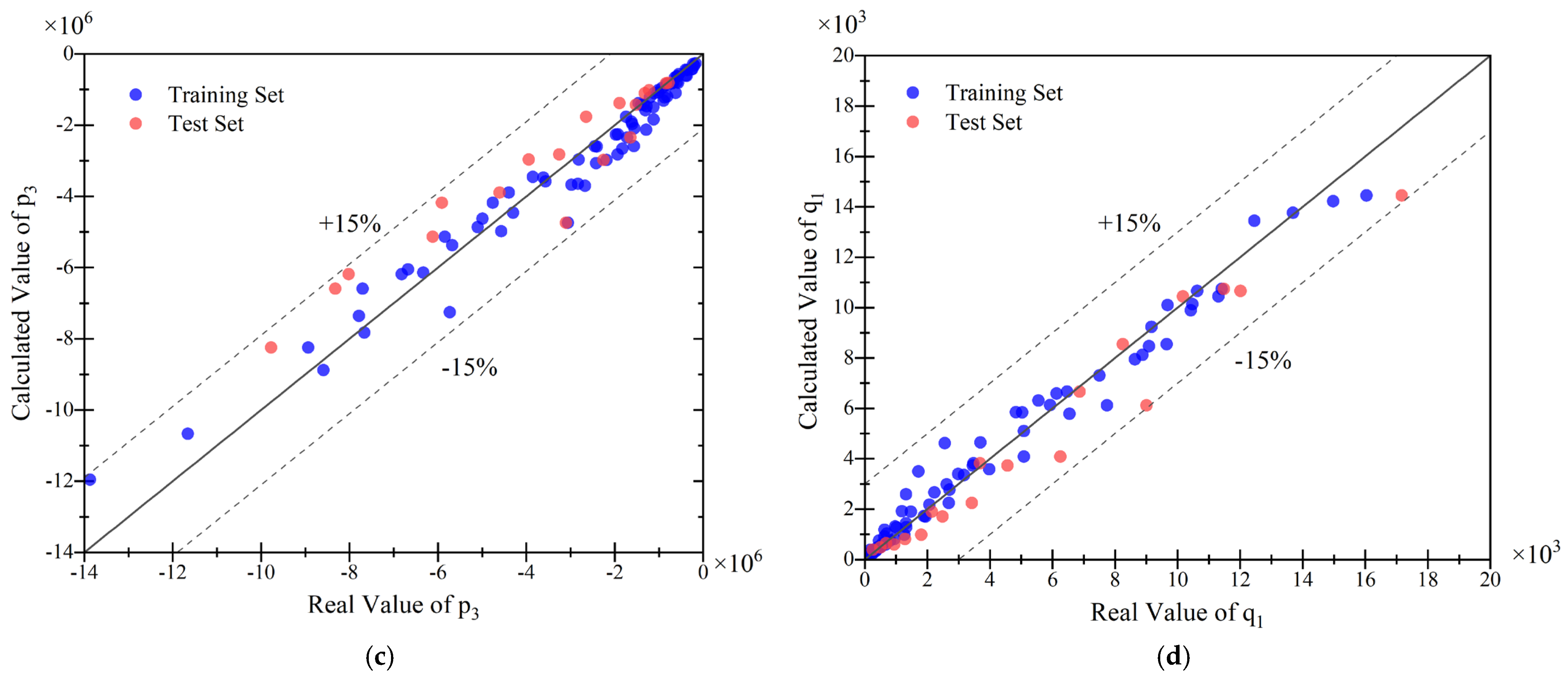
For the purpose of validating the accuracy of the quantitative relationship, a comparative analysis is conducted between the values of p₁, p₂, p₃ and q₁ obtained from fitting under experimental SRSs and the corresponding calculated values. Figure 11 illustrates the goodness-of-fit between the calculated and experimental values for the parameters p₁, p₂, p₃, and q₁. The blue points represent training data, while the red points represent testing data. The discrepancy between the experimental and calculated values lies within ±15%.

In this study, two metrics—R² and Mean Absolute Percentage Error (MAPE)—are adopted to evaluate the accuracy of the model. The formulas are shown in Equations (3) and (5).

$$\mathrm{MAPE}={\displaystyle \frac{1}{N}}{\displaystyle \sum _{i=1}^n\left|\frac{y_i-{\widehat{y}}_i}{y_i}\right|}$$

(5)

where ${\widehat{y}}_i$is the calculated value; $y_i$ is the real value; $\overline{y}$ is the mean of the real value; N is the number of data.

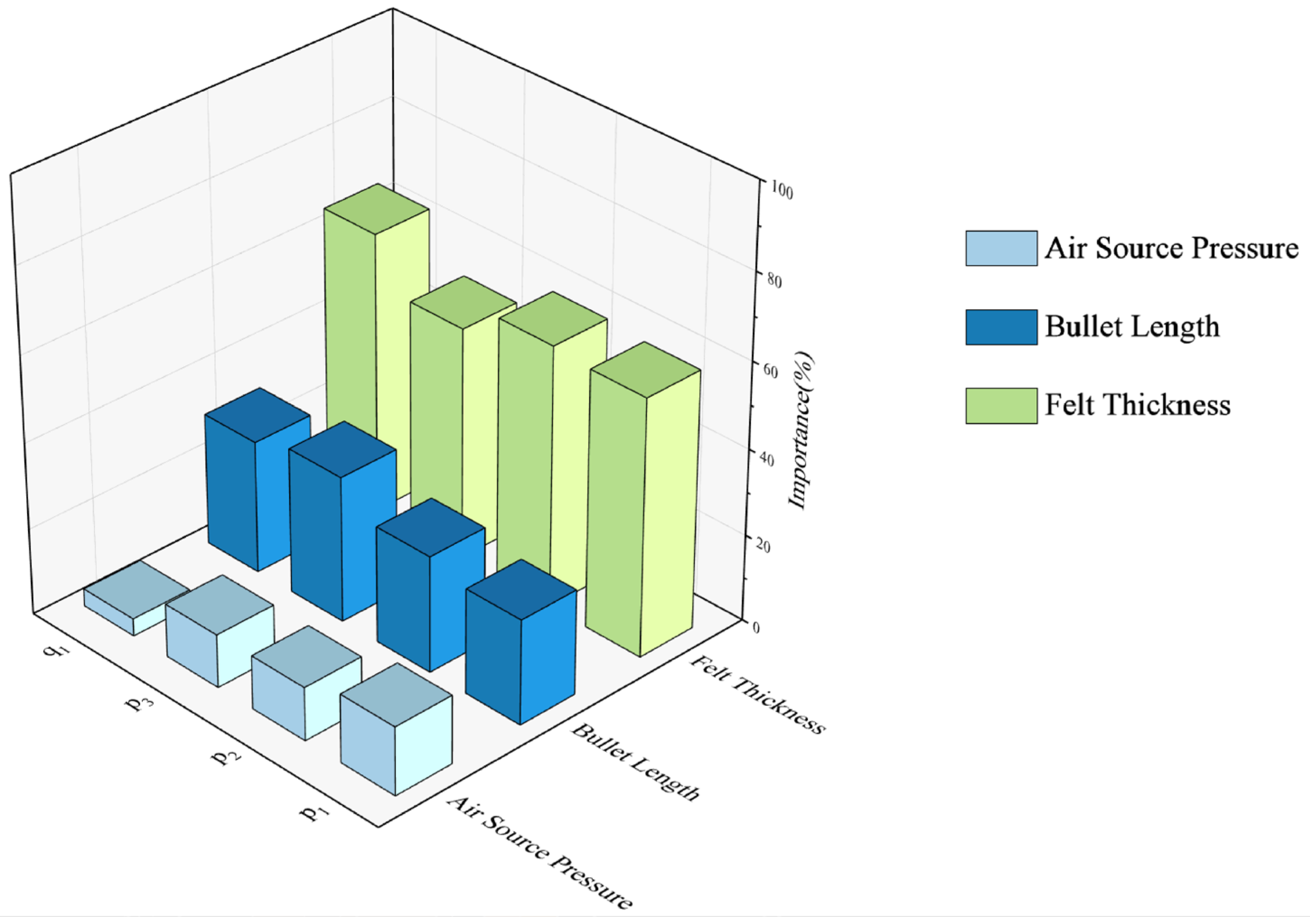
Based on calculations, the R² values for the quantitative relationship of p₁, p₂, p₃, and q₁ all exceed 0.8, and the MAPE values for these coefficients all remain around 0.2. It shows that the relationship has good accuracy and generalization effect. Figure 12 presents the importance ranking of shock parameters on the coefficients p₁, p₂, p₃, and q₁. It shows that the felt thickness has the greatest influence on the coefficients, while the air source pressure has the least influence. The felt thickness significantly influences the high-frequency amplitude; it has the greatest effect on the SRS pattern, resulting in the most substantial influence on the coefficients p₁, p₂, p₃, and q₁. In contrast, the air source pressure only influences the overall amplitude of the SRSs and has negligible effects on the pattern; consequently, it has the least influence on the coefficients. Since the bullet length affects both the low- and high-frequency regions of the SRSs, it exhibits the second largest influence on the coefficients.

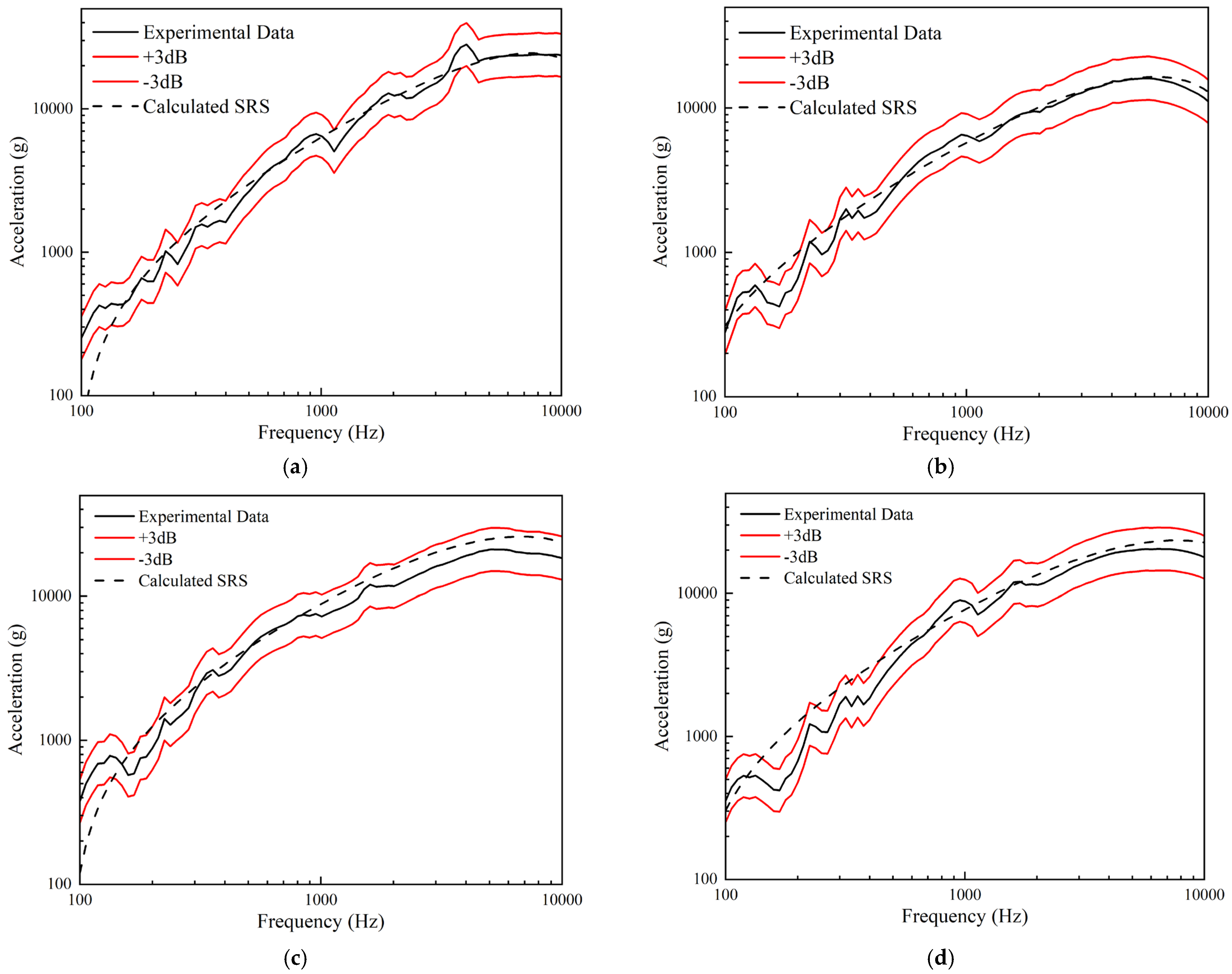
Validation experiments are conducted to rigorously assess the accuracy of the relationship. Figure 13a–d show the comparison between SRSs calculated by the RF algorithm and SRSs of the validation experiment. The solid black line in the figure represents the experimental SRSs, while the dashed black line demonstrates the calculated SRSs. It can be seen from the figure that the majority of the calculated SRS curves are within the tolerance range of ±3 dB of the experimental results. The discrepancy between calculated and experimental SRS is quantified by the MALE value. The MALE values between the calculated and experimental results are all below 10%, which are 7.23%, 5.30%, 9.92%, and 9.36%. The quantitative relationship demonstrates reliable calculation capability for SRS spectral patterns.

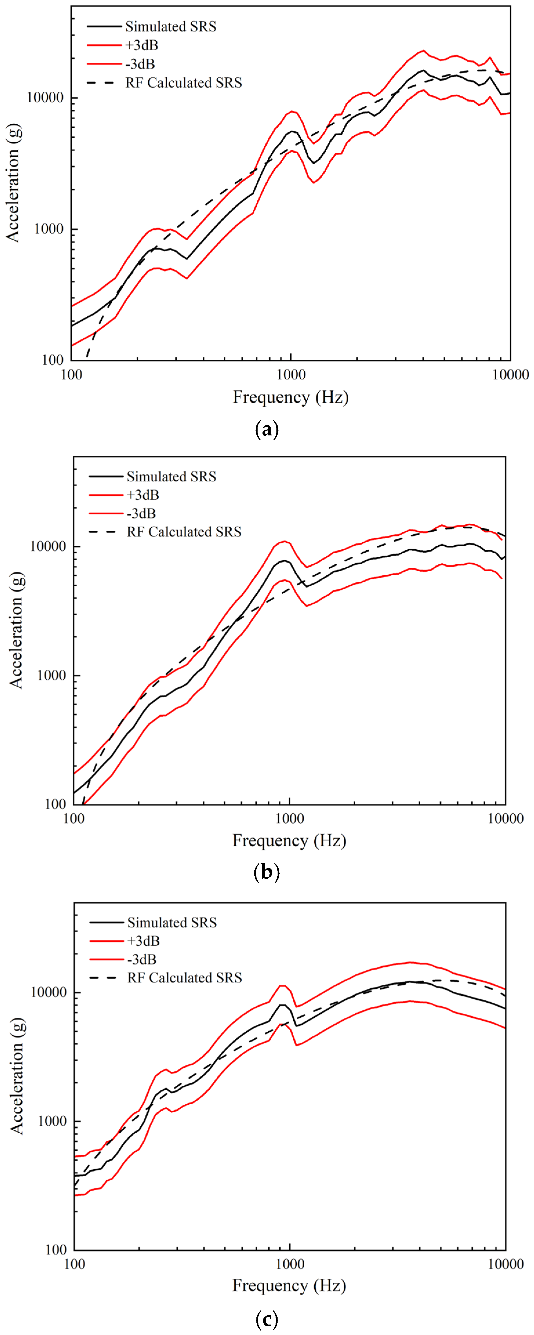
Furthermore, to further evaluate the generalization capability of the proposed model, additional validation was performed using three shock conditions that were not included in the training dataset. As shown in Figure 14a–c, the RF-based model can reasonably predict the SRS curves under previously unseen shock conditions, and the predicted results exhibit good agreement with the numerical simulation results. The MALE values are 11.81%, 12.68% and 6.27%. These results indicate that the proposed model can not only capture the SRS characteristics within the training dataset but also provide reliable predictions for shock conditions that were not included in the training process.

4.4. Applicability and Scope of the Quantitative Relationship Model

The quantitative relationship established in this study is developed based on the air- cannon-based shock device, and the three key shock parameters are investigated in this study. Therefore, the specific quantitative relationship established in this work should be applied within the three parameters and the present mechanical shock device. Its application to other shock devices or shock parameters would require further validation.

Nevertheless, the proposed methodology is not limited to the specific shock device. For a different resonate board configuration, the same experimental and numerical data-processing and random forest-based modeling procedure can be applied to establish a quantitative relationship.

Future studies will further investigate more advanced machine learning algorithms and incorporate additional shock parameters and structural parameters of the resonant plate to extend the parameter space and improve the general applicability of the proposed framework.

5. Conclusions

In this paper, experiments under different shock environments are carried out based on the air cannon device. Simulations of shock experiments under diverse parameters are also conducted using the LS-DYNA dynamics software. Then, the experimental and simulated SRSs are accurately fitted by MATLAB. A quantitative relationship is established for SRS calculation. Based on the findings and discussions presented, the conclusions are as follows:

• The spectral pattern of SRS is influenced by felt thickness, bullet length, and air source pressure. As felt thickness increases, the high-frequency amplitude and the knee frequency of the SRS decrease, whereas the low-frequency slope remains unchanged. The low-frequency regions of the SRS elevate with increasing bullet length, while the high-frequency amplitude decreases. When air source pressure rises, the SRS curve moves upward in all frequencies without altering its spectral pattern.
• By utilizing MATLAB, the SRSs under various experimental conditions can be effectively fitted. The R² values between fitted and experimental results are all above 0.8.
• Based on extensive experimental and simulated datasets, the random forest algorithm is employed to establish the quantitative relationship between the fitting equation coefficients (p₁, p₂, p₃ and q₁) and the three key shock parameters. The established model enables the SRS curves to be quantitatively calculated from the shock parameters. The model is experimentally validated, with the MALE values between the calculated and experimental SRSs below 10%, demonstrating its accuracy for efficient SRS calculation.

The SRS quantitative relationship in this study effectively resolves spectral calculation challenges under varied conditions of felt thickness, bullet length, and air source pressure. The relationship provides a valuable reference framework for enhancing the efficiency of pyroshock tests in aerospace engineering applications. It is worth noting that the quantitative relationship can rapidly calculate the SRS spectral pattern based on specified shock environments, but the quantitative relationship needs to be modified to be applicable to more complex conditions.

References

1. Filippi, E.; Cambier, F.; Conti, C. Development of the Alcatel ETCA pyroshock test facility. In Proceedings of the European Conference; ESA: Braunschweig, Germany, 1999; Available online: https://orbi.umons.ac.be/handle/20.500.12907/49690 (accessed on 13 September 2026).
2. Lee, J.R.; Chen, C.C.; Kong, C.W. Review of pyroshock wave measurement and simulation for space systems. Measurement 2012, 45, 631–642. [Google Scholar] [CrossRef] [Scilit]
3. Moening, C.J. Pyrotechnic shock flight failures. In IES Pyrotechnic Shock Tutorial Program, 31st ATM, Institute of Environmental Sciences; Institute of Environmental Sciences: Mount Prospect, IL, USA, 1985; Available online: https://www.vibrationdata.com/tutorials_alt/Pyrotechnic_Shock_Failures_Moening.pdf (accessed on 13 September 2026).
4. Mao, Y.J.; Li, Y.L. Advances in simulation techniques of pyroshock environments. Missile Space Veh. 2007, 4, 37–44. (In Chinese) [Google Scholar] [CrossRef]
5. Bai, M.; Thatcher, W. High G pyrotechnic shock simulation using metal-to-metal impact. Shock Vib. Bull. 1979, 49, 96–100. [Google Scholar]
6. Yan, H.; Qin, Z.; Zhang, W.; Ming, A.; Wang, X.; Chu, F. Dynamic analysis of laser shock response: Experimental and numerical studies. Aerosp. Sci. Technol. 2019, 94, 105430. [Google Scholar] [CrossRef] [Scilit]
7. NASA-STD-7003; Pyroshock Test Criteria. National Aeronautics and Space Administration: Washington, DC, USA, 1999. Available online: https://ntrs.nasa.gov/citations/20120000674 (accessed on 13 September 2026).
8. NASA-HDBK-7005; Dynamic Environmental Criteria. National Aeronautics and Space Administration: Washington, DC, USA, 2001. Available online: https://ntrs.nasa.gov/citations/20190026820 (accessed on 13 September 2026).
9. MIL-STD-810F; Department of Defense Test Method Standard for Environmental Engineering Considerations and Laboratory Tests. Department of Defense: Arlington, VA, USA, 2000. Available online: https://altronics.fr/fr/wp-content/uploads/altronics/MIL-STD-810F.pdf (accessed on 13 September 2026).
10. Zhao, H.D.; Sun, Y.; Ding, J.F.; Hao, Z.W.; Liu, W.; Wang, X.; Liu, Y.Z. Simulation techniques of pyroshock environment under the excitation of a light gas gun. J. Vib. Shock 2021, 40, 1–10. (In Chinese) [Google Scholar] [CrossRef]
11. Velmurugan, R.; Mohamed Najeeb, E. Study of far-field pyroshock responses of composite panels. J. Vib. Acoust. 2014, 136, 031014. [Google Scholar] [CrossRef] [Scilit]
12. Almesmari, A.; Jarrar, F.; Almaskari, F.; Marpu, P.R.; Shukoor, N.A.; Govindan, J.K. Development of a Metal-to-Metal Mid-Field Shock Test Procedure for Nanosatellites. IEEE J. Miniat. Air Sp. Syst. 2020, 1, 103–109. [Google Scholar] [CrossRef] [Scilit]
13. Wang, W.; Huang, K.S.; Zhao, F. Simulation of pyroshock environment and effect rules of shock response spectrum. Aeronaut. J. 2023, 127, 1659–1675. [Google Scholar] [CrossRef] [Scilit]
14. Chen, X.; Li, Z.W.; Xu, M.G.; He, Y.X.; Zhao, L. Shock response spectrum test based on twin gas gun impact test system. Spacecr. Environ. Eng. 2024, 41, 476–483. (In Chinese) [Google Scholar] [CrossRef]
15. Kim, B.S.; Lee, J. Development of impact test device for pyroshock simulation using impact analysis. Aerospace 2022, 9, 407. [Google Scholar] [CrossRef] [Scilit]
16. Yalçinkaya, T.; Gürsoy, B. Numerical Validation of a Pyroshock Test System and Application to Qualification Tests. Aerospace 2022, 9, 400. [Google Scholar] [CrossRef] [Scilit]
17. Viale, L.; Daga, A.P.; Fasana, A.; Garibaldi, L. On pyroshock tests for aerospace equipment qualification: A comprehensive parametric model for the simulation and the design of pyroshock test facilities. Int. J. Impact Eng. 2023, 180, 104697. [Google Scholar] [CrossRef] [Scilit]
18. Somasundaram, D.S.; Trabia, M.B.; O’Toole, B.J. A methodology for predicting high impact shock propagation within bolted-joint structures. Int. J. Impact Eng. 2014, 73, 30–42. [Google Scholar] [CrossRef] [Scilit]
19. Pi, B.L.; Zhang, J.H. Simulation study of pyroshock device testing using large plate. Struct. Environ. Eng. 2009, 36, 47–51. (In Chinese) [Google Scholar]
20. Hu, D.; Wang, H.; Huang, Z.; Xiao, W. Research on impact reduction of flexible boundary particle damping honeycomb plate based on discrete element multi body dynamics coupling. Electron. Res. Arch. 2023, 31, 6303–6326. [Google Scholar] [CrossRef] [Scilit]
21. Sun, W.; Huang, Y.; Chen, H. An improved adaptive genetic algorithm for optimizing pyroshock acceleration synthesis. IEEE Access 2019, 7, 132682–132693. [Google Scholar] [CrossRef] [Scilit]
22. Zhang, M.; Drikakis, D.; Li, L.; Yan, X. Machine-learning prediction of underwater shock loading on structures. Computation 2019, 7, 58. [Google Scholar] [CrossRef] [Scilit]
23. Zhou, J.M.; Dong, L.L.; Zhao, J.P.; Ding, Z.J.; Wang, X.Y. Method for response mapping prediction of aerospace structures based on probabilistic neural network. Spacecr. Environ. Eng. 2023, 40, 392–399. (In Chinese) [Google Scholar] [CrossRef]
24. Bae, W.; Park, J. Optimization of Pyroshock Test Conditions for Aerospace Components to Enhance Repeatability by Genetic Algorithms. Aerospace 2024, 11, 700. [Google Scholar] [CrossRef] [Scilit]
25. Blough, J.R.; DeClerck, J.; VanKarsen, C.; Soine, D.E. Method to predict the shock response spectrum shape from frequency response functions. In Proceedings of the 35th IMAC 2017; Springer International Publishing: Cham, Switzerland, 2017; pp. 177–185. [Google Scholar] [CrossRef] [Scilit]
26. Wang, X.; Liu, W.; Ding, J.; Sun, Y.; Dang, Y. Pyroshock response prediction of spacecraft structure in wide frequency domain based on acceleration FRF. Aerospace 2022, 9, 54. [Google Scholar] [CrossRef] [Scilit]
27. Tůma, J.; Kočí, P. Calculation of a shock response spectrum. In Proceedings of the 12th International Carpathian Control Conference (ICCC), Velké Karlovice, Czech Republic, 25–28 May 2011; pp. 404–409. [Google Scholar] [CrossRef] [Scilit]
28. Harris, C.M.; Piersol, A.G. Shock and Vibration Handbook; McGraw-Hill: New York, NY, USA, 2002; Available online: https://www.accessengineeringlibrary.com/content/book/9780071508193 (accessed on 13 September 2026).
Figure 1. Air cannon device. (a) Schematic diagram. (b) Physical diagram.
Aerospace 13 00840 g001
Figure 2. Comparison of SRSs under identical shock environment.
Aerospace 13 00840 g002
Figure 3. Bullet size.
Aerospace 13 00840 g003
Figure 4. Finite element model. (a) Front view. (b) Vertical view.
Aerospace 13 00840 g004
Figure 5. SRSs under different grid conditions.
Aerospace 13 00840 g005
Figure 6. SRSs under different felt thicknesses condition.
Aerospace 13 00840 g006
Figure 7. SRSs under different air source pressure conditions.
Aerospace 13 00840 g007
Figure 8. SRSs under different bullet length conditions.
Aerospace 13 00840 g008
Figure 9. Comparison of fitting results of different curves. (The red star in the figure denotes the rational function fitting curve with the maximum R2 value.)
Aerospace 13 00840 g009
Figure 10. Fitting curves under different shock parameters conditions. (a) Different felt thicknesses. (b) Different bullet lengths. (c) Different air source pressures.
Aerospace 13 00840 g010aAerospace 13 00840 g010b
Figure 11. The discrepancy of real and calculated values of different coefficients. (a) p1; (b) p2; (c) p3; (d) q1.
Aerospace 13 00840 g011aAerospace 13 00840 g011b
Figure 12. Variable importance ranking.
Aerospace 13 00840 g012
Figure 13. Comparison between experimental SRSs and calculated SRSs. (a) P = 0.7 MPa, h = 70 mm, D = 0 mm; (b) P = 0.7 MPa, h = 120 mm, D = 5 mm; (c) P = 0.9 MPa, h = 200 mm, D = 0 mm; (d) P = 0.9 MPa, h = 70 mm, D = 10 mm.
Aerospace 13 00840 g013
Figure 14. Comparison between simulated SRSs and calculated SRSs. (a) P = 0.4 MPa, h = 70 mm, D = 0 mm; (b) P = 0.5 MPa, h = 80 mm, D = 5 mm; (c) P = 0.7 MPa, h = 200 mm, D = 4 mm.
Aerospace 13 00840 g014