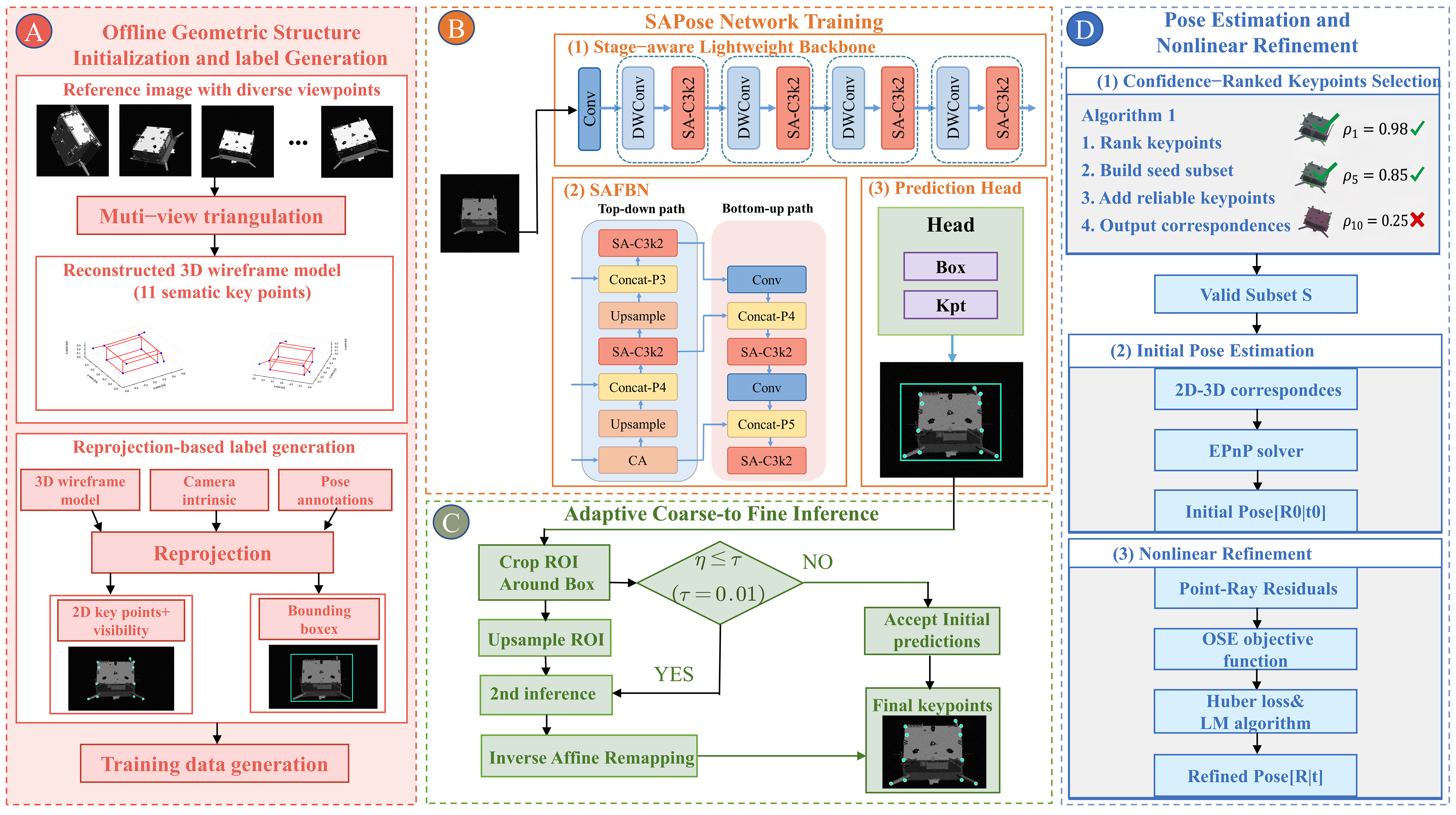
Figure 1.
Overall pipeline of the proposed indirect pose-estimation framework: (A) offline geometric structure initialization and label generation; (B) SAPose network training; (C) adaptive coarse-to-fine inference; (D) pose estimation and nonlinear refinement.
Figure 1.
Overall pipeline of the proposed indirect pose-estimation framework: (A) offline geometric structure initialization and label generation; (B) SAPose network training; (C) adaptive coarse-to-fine inference; (D) pose estimation and nonlinear refinement.
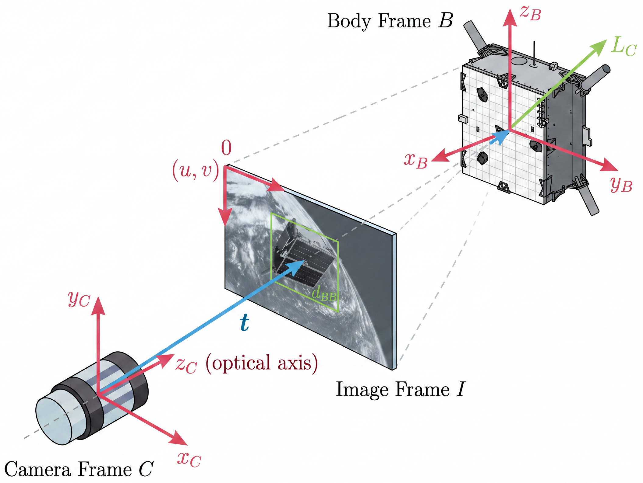
Figure 2.
Coordinate systems and relative-pose geometry. B: target body frame; C: camera frame centered at the optical center; I: image plane.
Figure 2.
Coordinate systems and relative-pose geometry. B: target body frame; C: camera frame centered at the optical center; I: image plane.
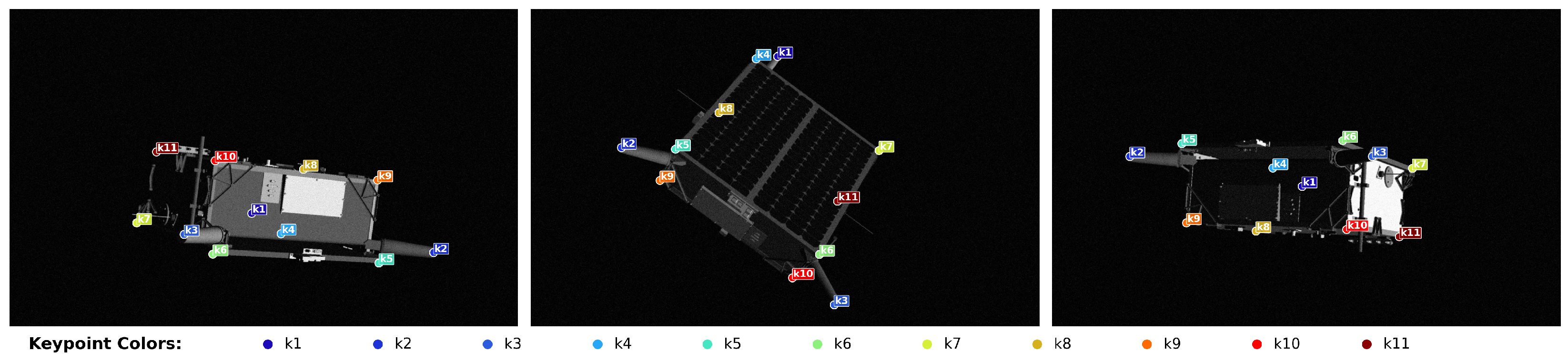
Figure 3.
Reference images for semantic landmark annotation. Numbers 1–11 denote the 11 predefined semantic landmarks used to construct the sparse 3D spacecraft model.
Figure 3.
Reference images for semantic landmark annotation. Numbers 1–11 denote the 11 predefined semantic landmarks used to construct the sparse 3D spacecraft model.
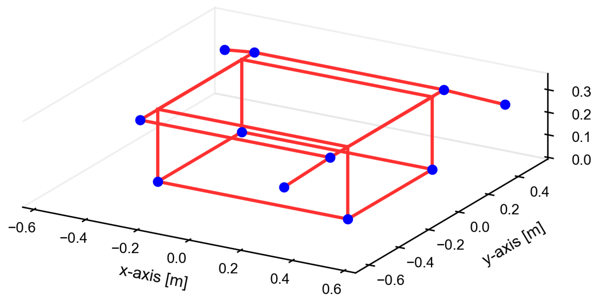
Figure 4.
Reconstructed sparse 3D wireframe model with 11 landmarks.
Figure 4.
Reconstructed sparse 3D wireframe model with 11 landmarks.
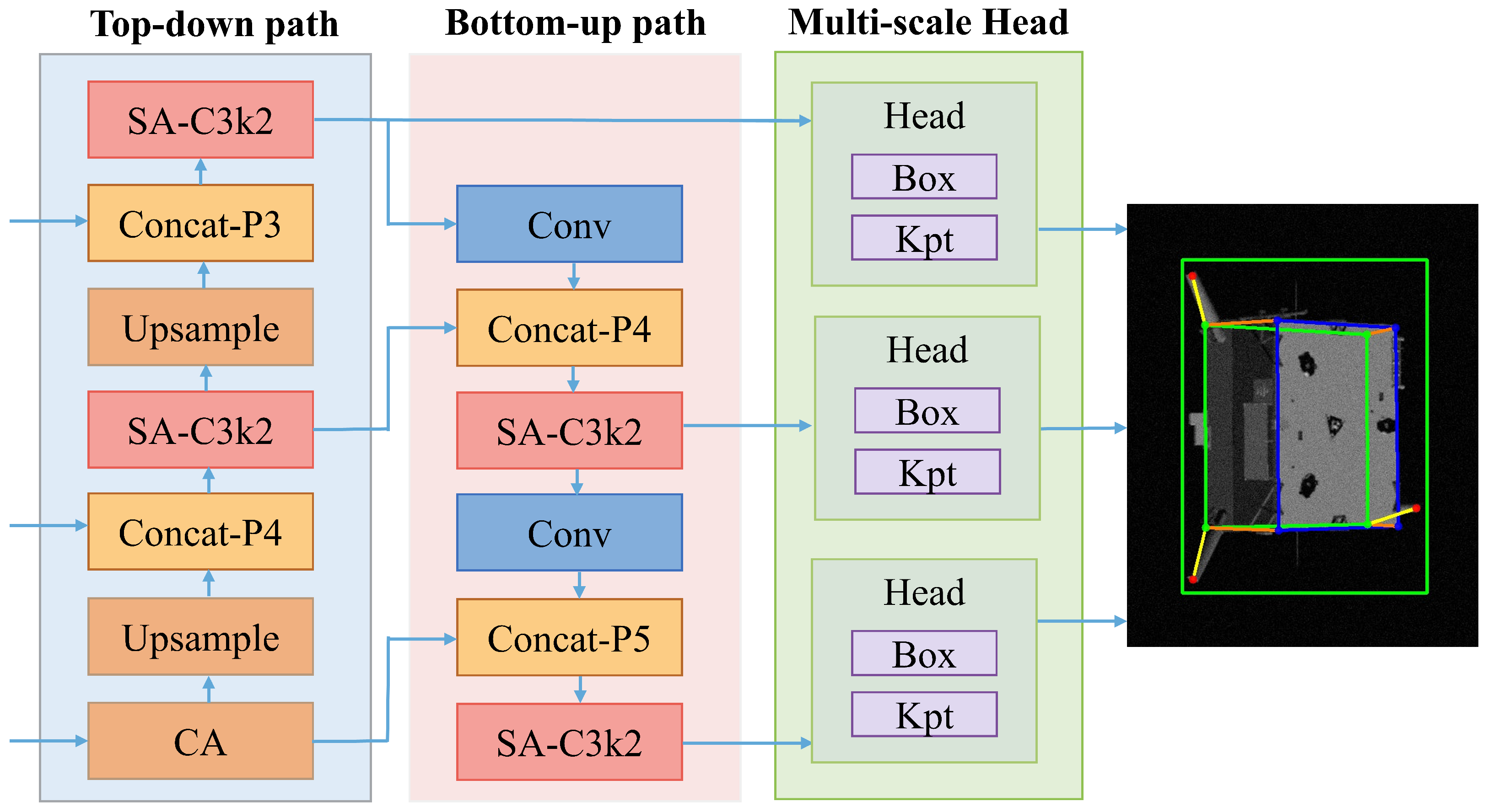
Figure 5.
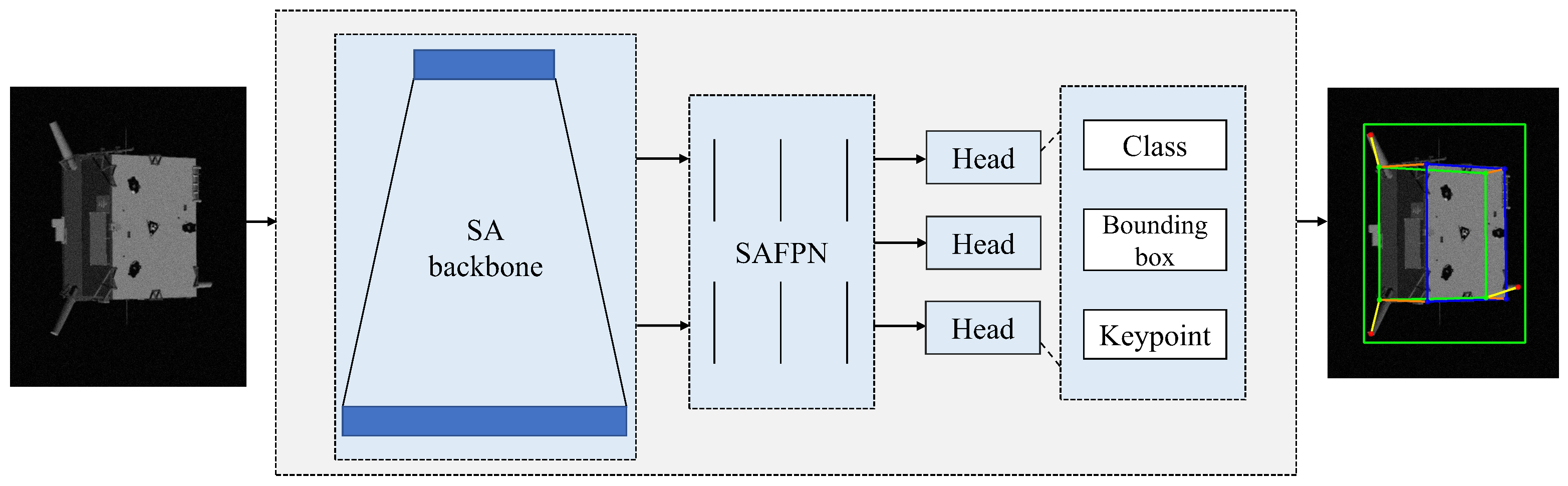
Overall SAPose architecture. A stage-aware lightweight backbone extracts hierarchical features, SAFPN fuses multi-scale features, and task-specific heads predict the spacecraft class, bounding box, and 2D keypoints.
Figure 5.
Overall SAPose architecture. A stage-aware lightweight backbone extracts hierarchical features, SAFPN fuses multi-scale features, and task-specific heads predict the spacecraft class, bounding box, and 2D keypoints.
Figure 6.
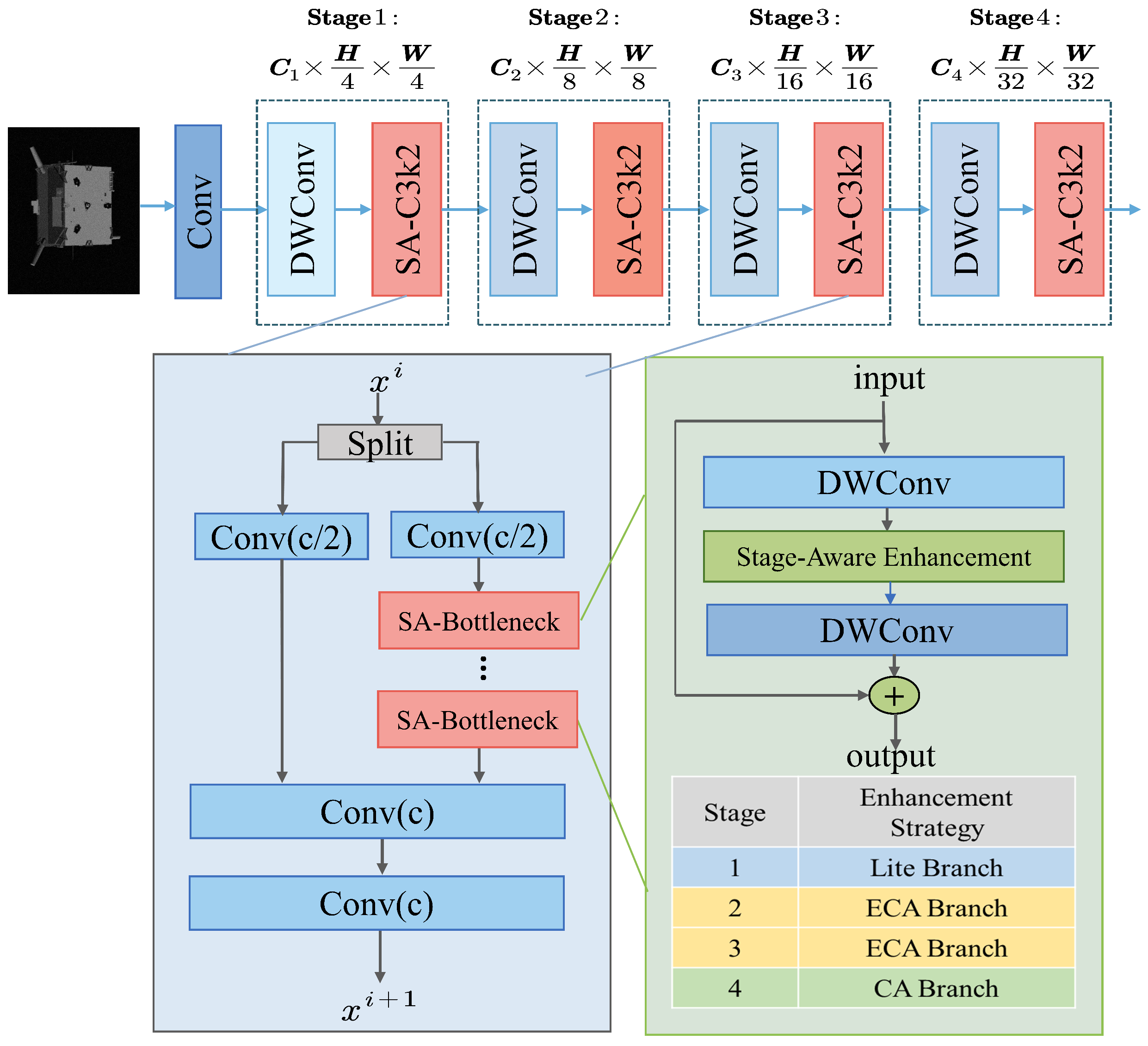
Stage-aware lightweight backbone. Each stage comprises a DWConv layer and an SA-C3k2 block; SA-C3k2 uses dual branches with stacked SA-Bottlenecks and stage-specific enhancement.
Figure 6.
Stage-aware lightweight backbone. Each stage comprises a DWConv layer and an SA-C3k2 block; SA-C3k2 uses dual branches with stacked SA-Bottlenecks and stage-specific enhancement.
Figure 7.
SAPose neck and head structure. SAFPN fuses P3–P5 through top-down and bottom-up paths for small-, medium-, and large-scale targets. Right: C3k2, upsampling, and convolution blocks.
Figure 7.
SAPose neck and head structure. SAFPN fuses P3–P5 through top-down and bottom-up paths for small-, medium-, and large-scale targets. Right: C3k2, upsampling, and convolution blocks.
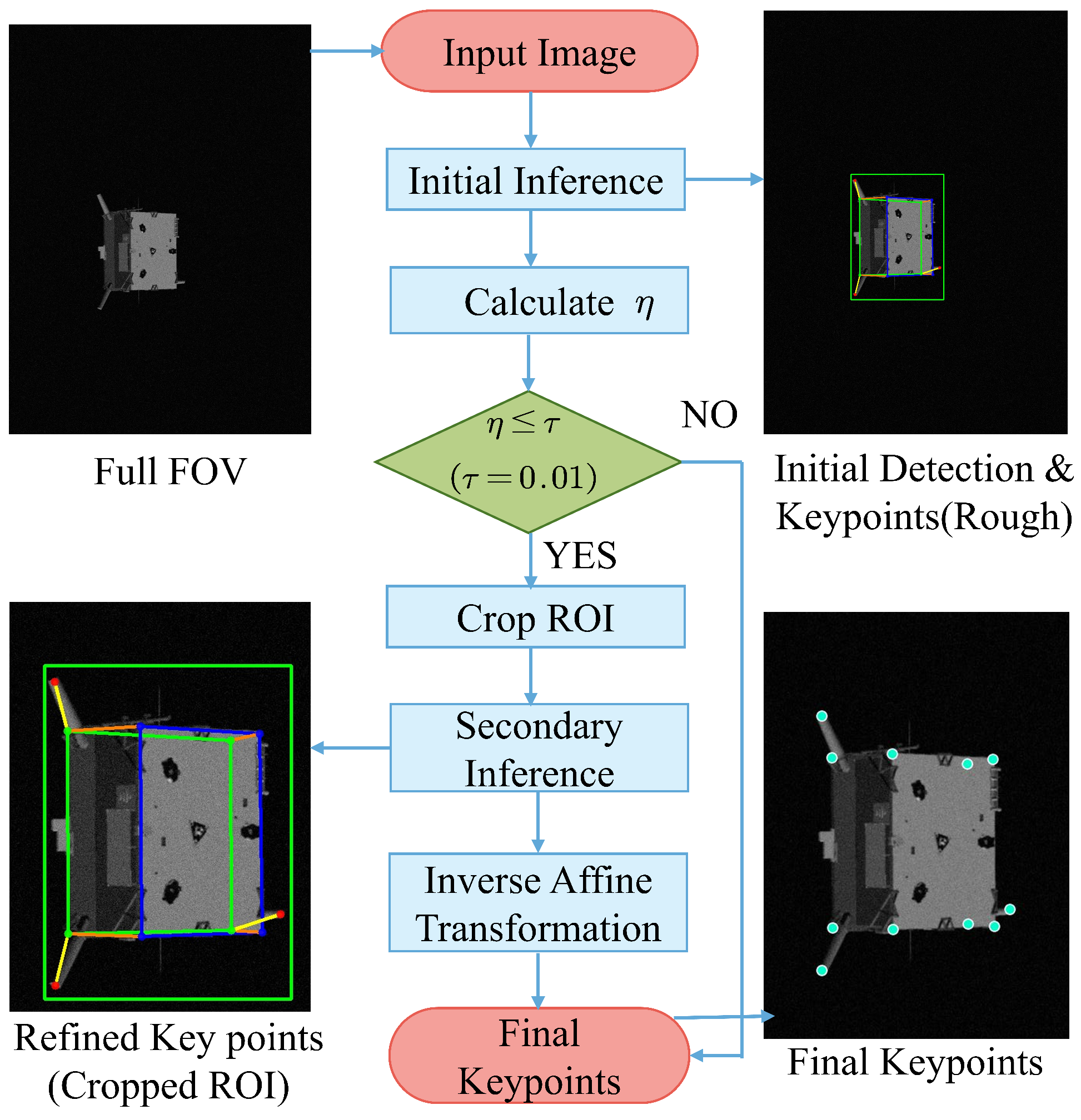
Figure 8.
Conditional coarse-to-fine inference. Targets with undergo at most one ROI refinement pass, and the refined keypoints are mapped back to the full image. If refinement is unavailable or invalid, the valid first-pass prediction is retained.
Figure 8.
Conditional coarse-to-fine inference. Targets with undergo at most one ROI refinement pass, and the refined keypoints are mapped back to the full image. If refinement is unavailable or invalid, the valid first-pass prediction is retained.
Figure 9.
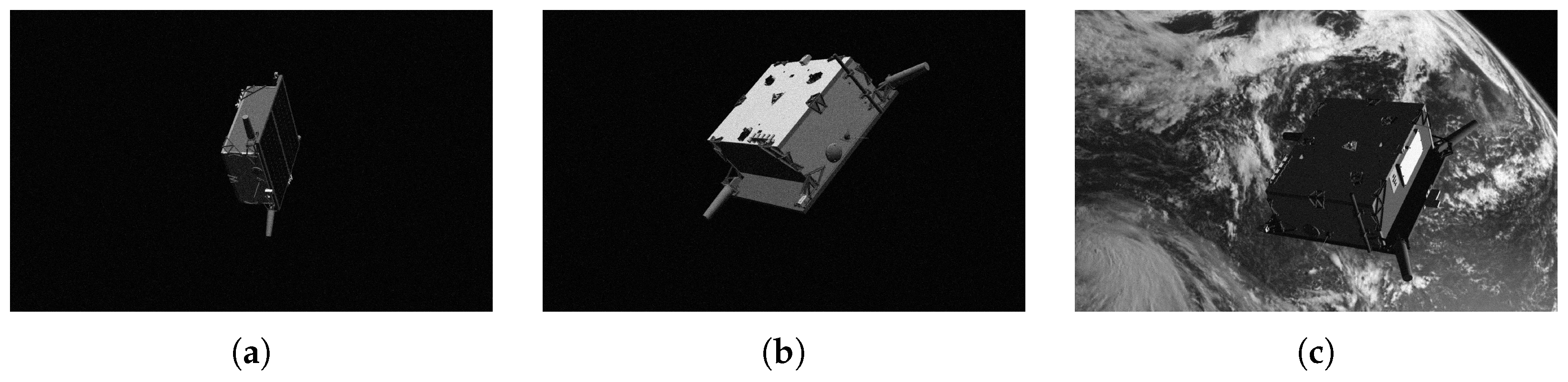
Examples from SPEED under varying illumination, background, distance, and viewpoint. (a) img001491. (b) img005179. (c) img014352.
Figure 9.
Examples from SPEED under varying illumination, background, distance, and viewpoint. (a) img001491. (b) img005179. (c) img014352.
Figure 10.
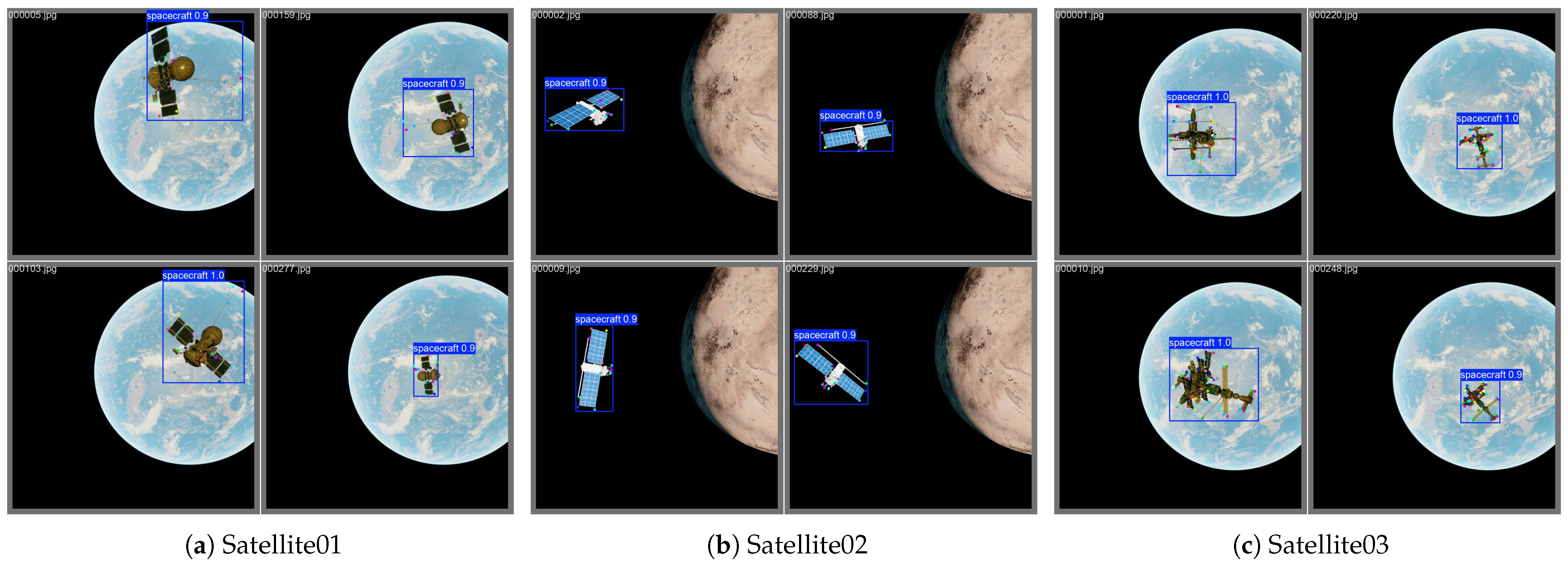
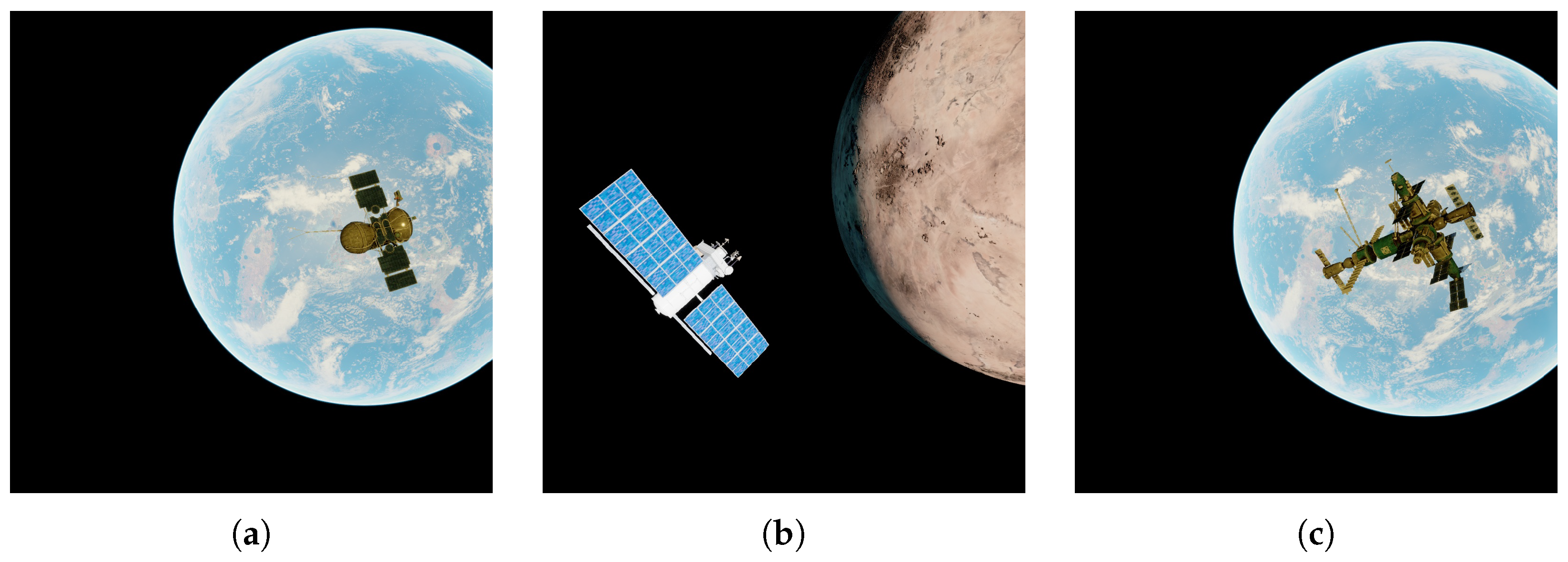
Spacecraft models in SKD. (a) Satellite01. (b) Satellite02. (c) Satellite03.
Figure 10.
Spacecraft models in SKD. (a) Satellite01. (b) Satellite02. (c) Satellite03.
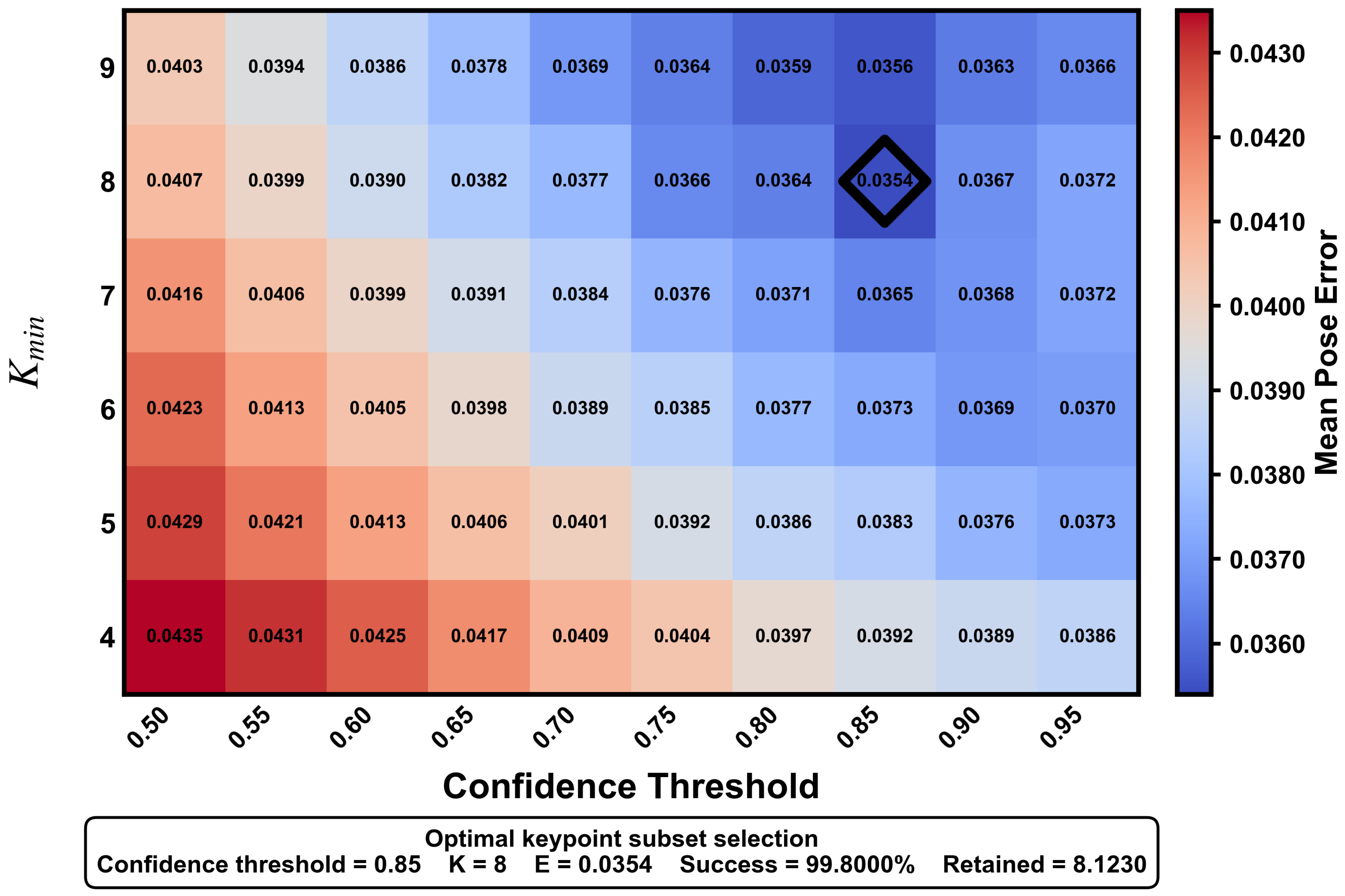
Figure 11.
Validation mean pose error over keypoint-selection hyperparameters with . The axes denote confidence threshold and minimum retained keypoints ; the black diamond marks the selected optimum, and .
Figure 11.
Validation mean pose error over keypoint-selection hyperparameters with . The axes denote confidence threshold and minimum retained keypoints ; the black diamond marks the selected optimum, and .
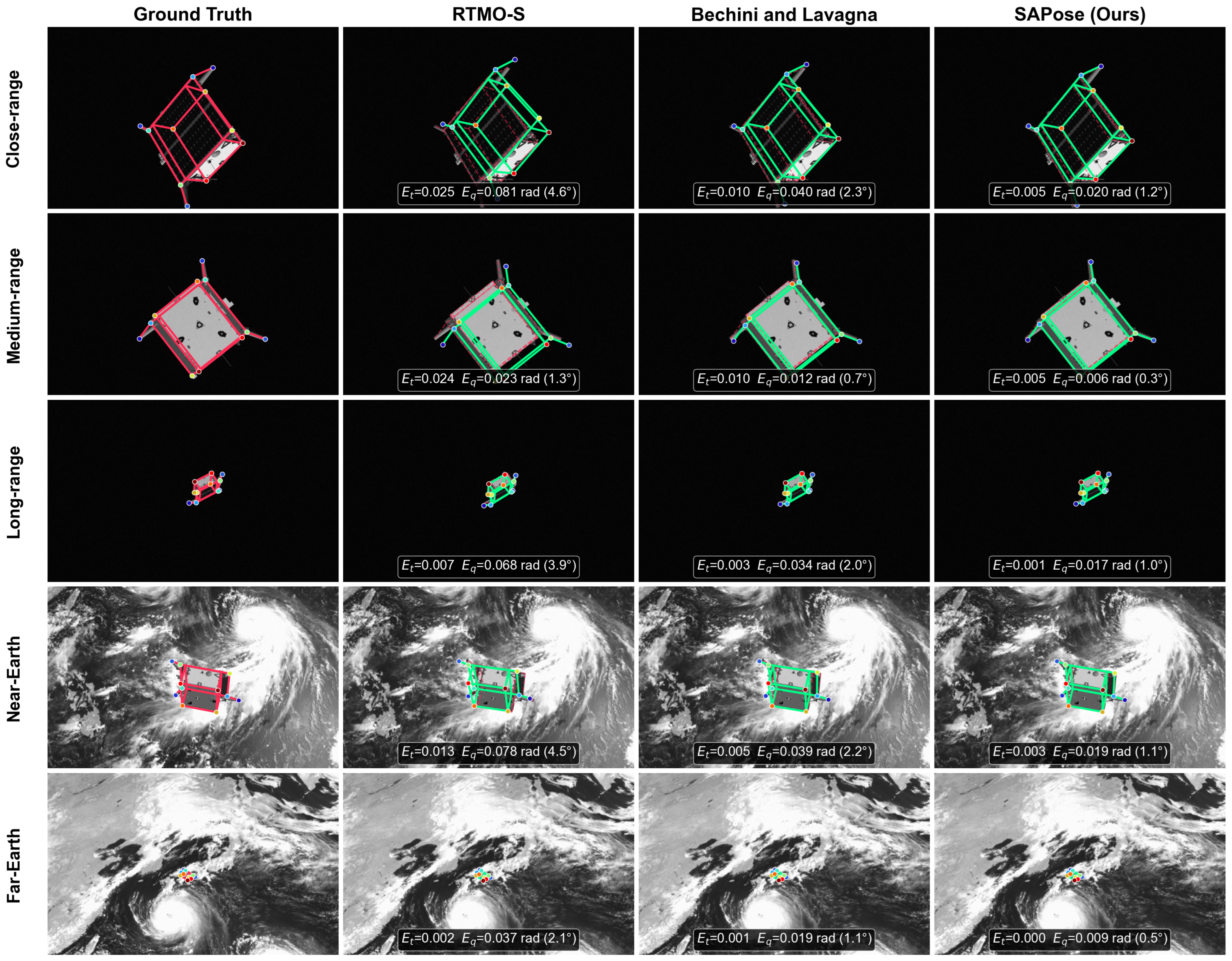
Figure 12.
Qualitative comparison on five representative SPEED scenarios. Rows 1–5: close-range, medium-range, long-range, near-Earth, and far-Earth observations. Columns: ground truth, RTMO-S, Bechini & Lavagna, and SAPose. Red and green wireframes denote ground truth and estimated pose, respectively; colored dots mark predicted 2D keypoints. and (rad) are shown below each prediction.
Figure 12.
Qualitative comparison on five representative SPEED scenarios. Rows 1–5: close-range, medium-range, long-range, near-Earth, and far-Earth observations. Columns: ground truth, RTMO-S, Bechini & Lavagna, and SAPose. Red and green wireframes denote ground truth and estimated pose, respectively; colored dots mark predicted 2D keypoints. and (rad) are shown below each prediction.
Figure 13.
SAPose keypoint predictions on the three SKD spacecraft targets. Colored dots denote the predicted 2D semantic keypoints.
Figure 13.
SAPose keypoint predictions on the three SKD spacecraft targets. Colored dots denote the predicted 2D semantic keypoints.
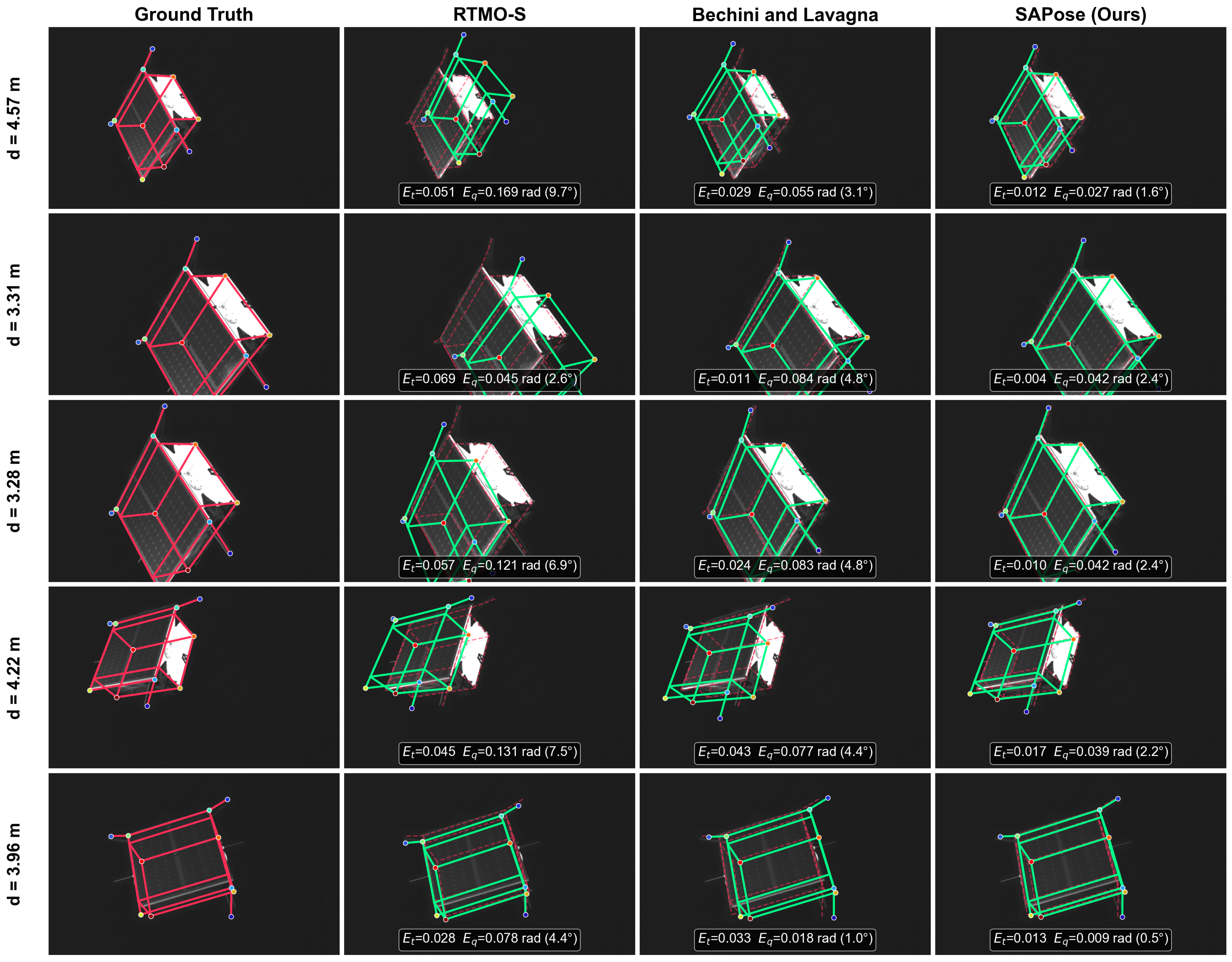
Figure 14.
Synthetic-to-real evaluation on five real SPEED images. All methods are trained on synthetic SPEED data and evaluated without real-image fine-tuning or adaptation. Rows correspond to the five images; columns show ground truth, RTMO-S, Bechini & Lavagna, and SAPose. Red and green wireframes denote Vicon ground truth and estimated pose, respectively; and are shown below each prediction.
Figure 14.
Synthetic-to-real evaluation on five real SPEED images. All methods are trained on synthetic SPEED data and evaluated without real-image fine-tuning or adaptation. Rows correspond to the five images; columns show ground truth, RTMO-S, Bechini & Lavagna, and SAPose. Red and green wireframes denote Vicon ground truth and estimated pose, respectively; and are shown below each prediction.
Figure 15.
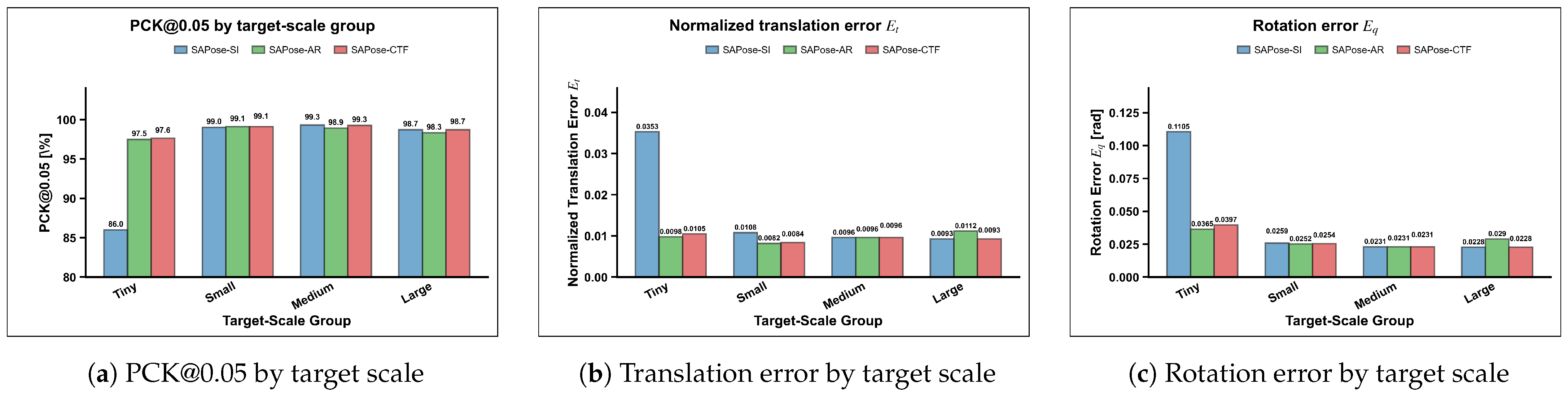
Performance comparison among SAPose-SI, SAPose-AR, and SAPose-CTF across different target-scale groups.
Figure 15.
Performance comparison among SAPose-SI, SAPose-AR, and SAPose-CTF across different target-scale groups.
Figure 16.
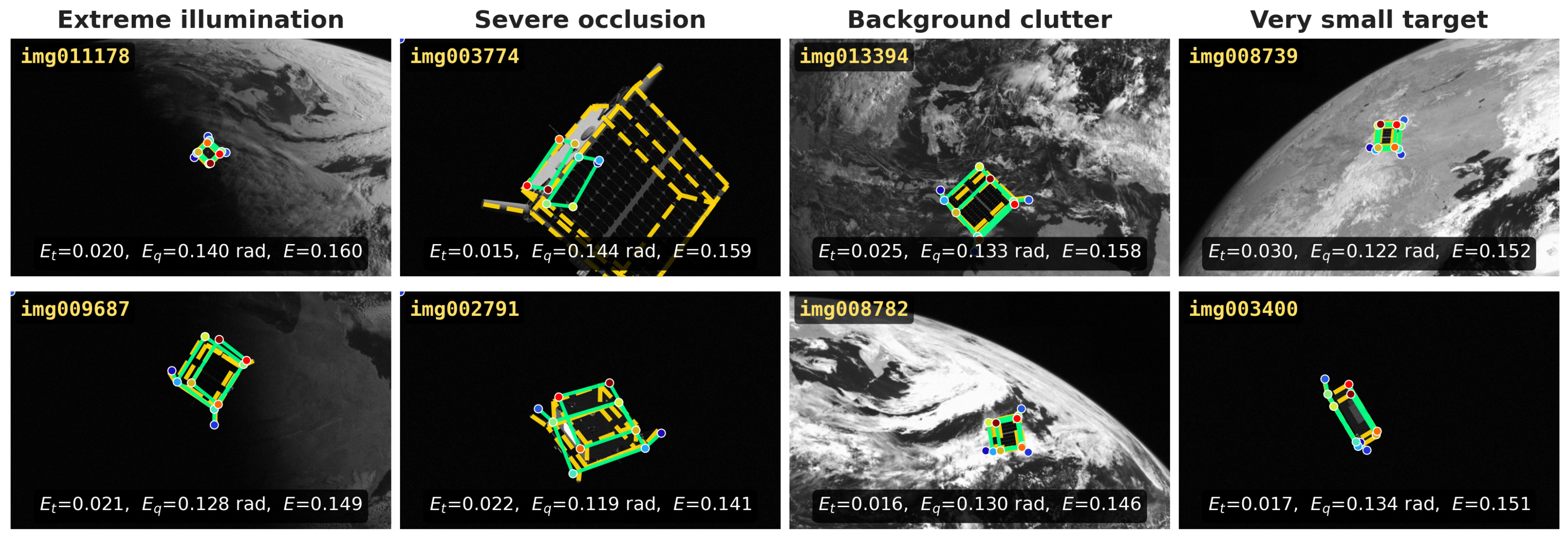
Representative SAPose failure cases on SPEED under extreme illumination, severe occlusion, background clutter, and very small target scale (columns). Yellow dashed and green solid wireframes denote the ground-truth projection and the predicted 11-keypoint configuration, respectively; , , and are shown below each image.
Figure 16.
Representative SAPose failure cases on SPEED under extreme illumination, severe occlusion, background clutter, and very small target scale (columns). Yellow dashed and green solid wireframes denote the ground-truth projection and the predicted 11-keypoint configuration, respectively; , , and are shown below each image.
Figure 17.
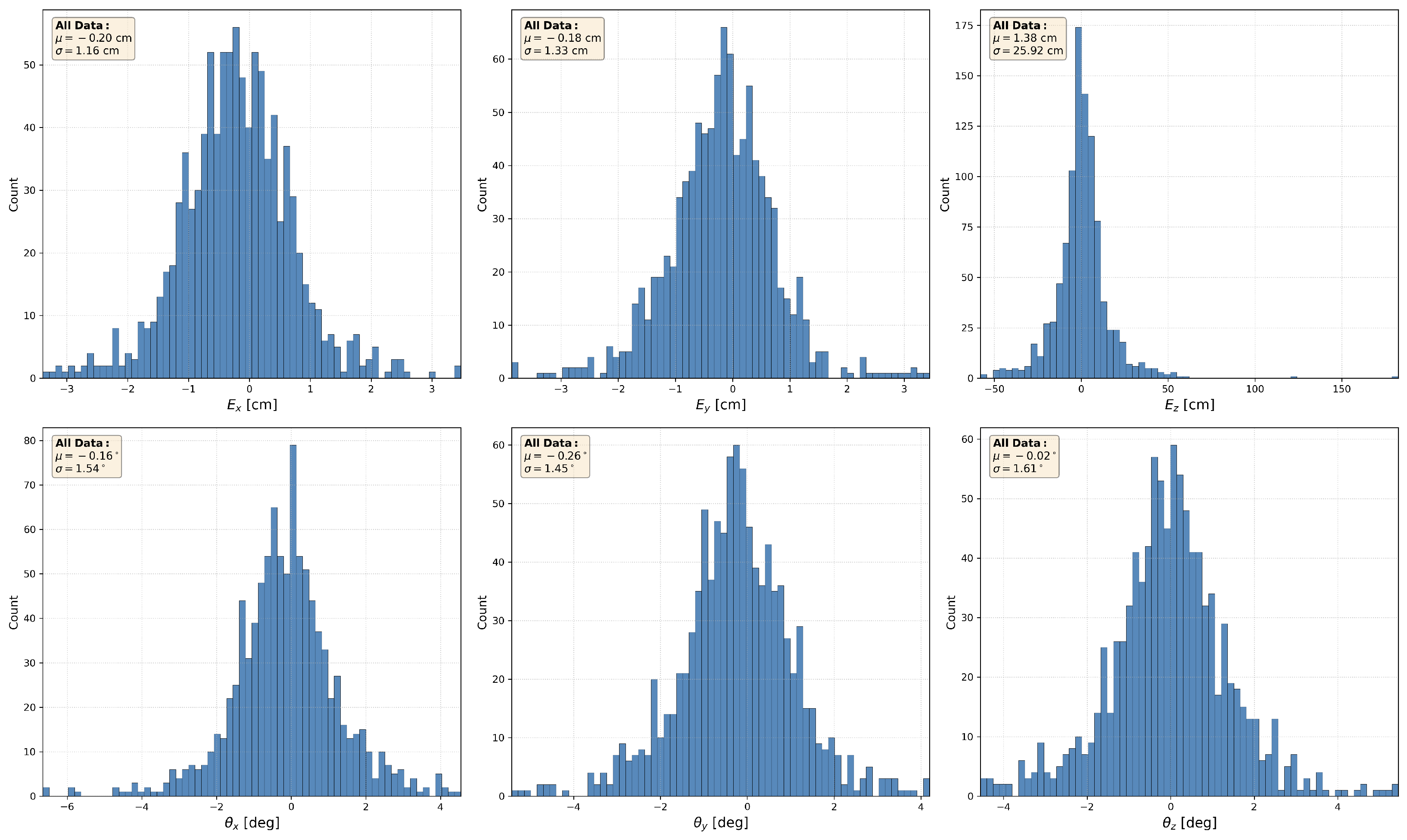
Component-wise SAPose error distributions on SPEED. The upper row shows translation errors along the camera-frame axes; the lower row shows Euler-angle attitude errors.
Figure 17.
Component-wise SAPose error distributions on SPEED. The upper row shows translation errors along the camera-frame axes; the lower row shows Euler-angle attitude errors.
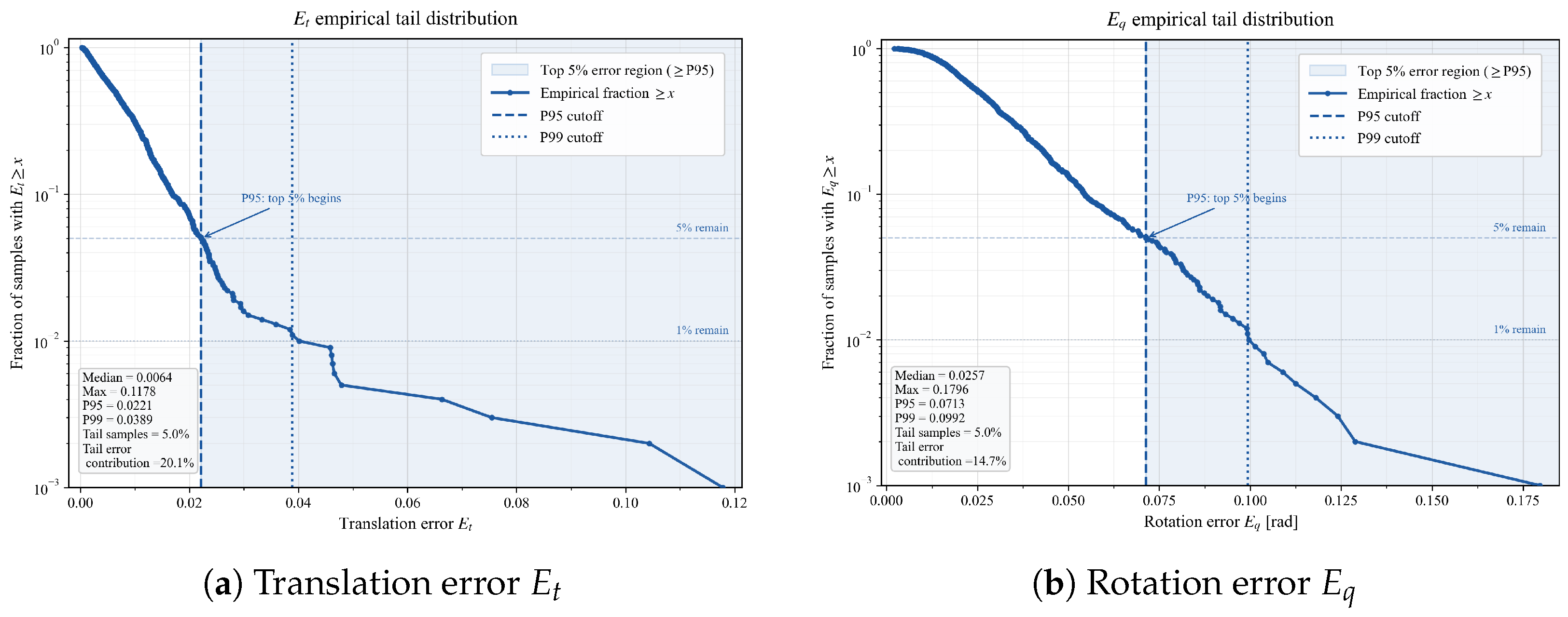
Figure 18.
Empirical SAPose error-tail distributions on SPEED. The panels show the fraction of samples with or greater than or equal to threshold x; shaded regions mark the top 5% beyond the corresponding P95 thresholds.
Figure 18.
Empirical SAPose error-tail distributions on SPEED. The panels show the fraction of samples with or greater than or equal to threshold x; shaded regions mark the top 5% beyond the corresponding P95 thresholds.
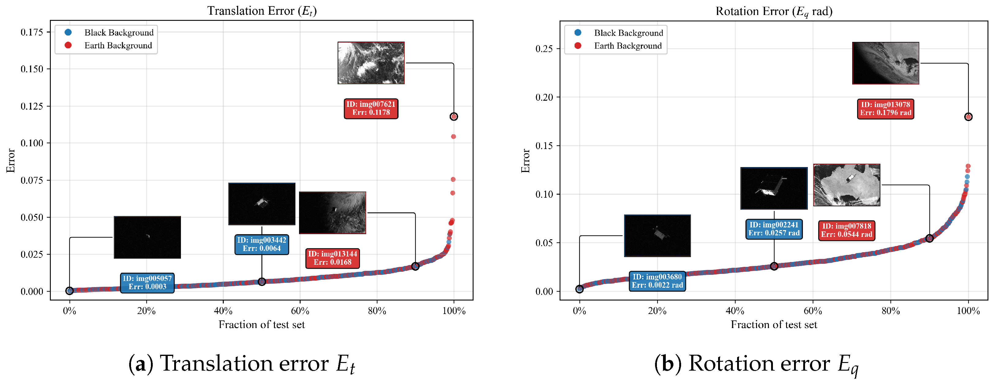
Figure 19.
Sorted SAPose pose-error distributions under black- and Earth-background conditions on SPEED. The panels show normalized translation error and rotation error .
Figure 19.
Sorted SAPose pose-error distributions under black- and Earth-background conditions on SPEED. The panels show normalized translation error and rotation error .
Table 1.
Training hyperparameter configuration.
Table 1.
Training hyperparameter configuration.
| Parameter | Value |
|---|
| Optimizer | AdamW |
| Initial Learning Rate | 1 × 10⁻³ |
| Learning Rate Scheduler | Cosine Annealing |
| Batch Size | 24 |
| Epochs | 250 |
| Input Image Size | 512 × 512 |
| Momentum | 0.88 |
| Weight Decay | 3.8 × 10⁻⁴ |
| Data Augmentation | Mosaic 0.9, Hue/Saturation/Brightness |
Table 2.
Validation-set sensitivity analysis of the target-occupancy threshold . Results are reported as the mean ± SD over five training seeds (0–4), with and fixed throughout the sweep.
Table 2.
Validation-set sensitivity analysis of the target-occupancy threshold . Results are reported as the mean ± SD over five training seeds (0–4), with and fixed throughout the sweep.
| Trigger Ratio (%) | PCK@0.05 ↑ | Et ↓ | Eq ↓ | E ↓ | Latency (ms) ↓ |
|---|
| 0.0050 | 15.1 ± 0.5 | 96.82 ± 0.24 | 0.0124 ± 0.0009 | 0.0389 ± 0.0025 | 0.0513 ± 0.0031 | 10.74 ± 0.27 |
| 0.0075 | 24.3 ± 0.7 | 97.96 ± 0.18 | 0.0099 ± 0.0007 | 0.0327 ± 0.0020 | 0.0426 ± 0.0025 | 11.61 ± 0.30 |
| 0.0100 | 33.2 ± 0.8 | 98.55 ± 0.14 | 0.0077 ± 0.0005 | 0.0277 ± 0.0012 | 0.0354 ± 0.0015 | 12.50 ± 0.34 |
| 0.0125 | 42.5 ± 1.0 | 98.61 ± 0.13 | 0.0073 ± 0.0005 | 0.0278 ± 0.0013 | 0.0351 ± 0.0016 | 13.39 ± 0.37 |
| 0.0150 | 51.0 ± 1.2 | 98.63 ± 0.12 | 0.0072 ± 0.0006 | 0.0278 ± 0.0014 | 0.0350 ± 0.0017 | 14.24 ± 0.40 |
Table 3.
Controlled comparison with recent lightweight keypoint estimation methods on the SPEED test subset (n = 1000). The architecture column identifies CNN, Transformer-based, and hybrid representatives. Trainable methods are reported as the mean ± SD over five independent runs, and the best entry per column is bolded. ViTPose-S provides a Transformer-based controlled baseline, while RTMO-S and ProbPose-S provide lightweight- and accuracy-oriented reference points, respectively.
Table 3.
Controlled comparison with recent lightweight keypoint estimation methods on the SPEED test subset (n = 1000). The architecture column identifies CNN, Transformer-based, and hybrid representatives. Trainable methods are reported as the mean ± SD over five independent runs, and the best entry per column is bolded. ViTPose-S provides a Transformer-based controlled baseline, while RTMO-S and ProbPose-S provide lightweight- and accuracy-oriented reference points, respectively.
| Method | Architecture | Source | Params (M) | PCK@0.05 ↑ | OKS-mAP ↑ |
|---|
| YOLO-Pose-S | CNN | CVPRW 2022 [26] | ∼10.0 | 92.32 ± 0.09 | 85.27 ± 0.11 |
| KAPAO-S | CNN-based | ECCV 2022 [27] | 12.6 | 94.71 ± 0.14 | 88.06 ± 0.11 |
| ViTPose-S | Vision Transformer | NeurIPS 2022 [28] | ∼22.0 | 96.38 ± 0.13 | 91.13 ± 0.14 |
| RTMO-S | Hybrid/lightweight | CVPR 2024 [29] | 9.9 | 96.95 ± 0.12 | 92.08 ± 0.10 |
| ProbPose-S | Probabilistic/hybrid | CVPR 2025 [30] | ∼24.0 | 97.62 ± 0.15 | 93.16 ± 0.14 |
| SAPose (Ours) | CNN + geometry | – | 9.4 | 98.58 ± 0.13 | 94.03 ± 0.14 |
Table 4.
Statistical analysis of the pre-specified primary keypoint comparisons on SPEED. OKS-mAP is computed once per trained checkpoint, and two-sided paired t-tests are performed across five matched training seeds (n = 5, df = 4). Positive differences indicate higher OKS-mAP for SAPose. Holm-adjusted p-values are reported for the two-comparison family.
Table 4.
Statistical analysis of the pre-specified primary keypoint comparisons on SPEED. OKS-mAP is computed once per trained checkpoint, and two-sided paired t-tests are performed across five matched training seeds (n = 5, df = 4). Positive differences indicate higher OKS-mAP for SAPose. Holm-adjusted p-values are reported for the two-comparison family.
| Comparison | Mean ΔOKS-mAP (pp) | 95% CI | padj |
|---|
| SAPose vs. RTMO-S | +1.95 | [+1.70, +2.20] | 5.1 × 10⁻⁵ |
| SAPose vs. ProbPose-S | +0.87 | [+0.56, +1.18] | 1.4 × 10⁻³ |
Table 5.
Controlled results for representative spacecraft-specific pose-estimation methods on the SPEED held-out labeled subset (n = 1000), with additional literature-only reference values reported under their original protocols. Reproducible methods are reported as the mean ± SD over five independent training runs. The best reproducible result in each error column is bolded.
Table 5.
Controlled results for representative spacecraft-specific pose-estimation methods on the SPEED held-out labeled subset (n = 1000), with additional literature-only reference values reported under their original protocols. Reproducible methods are reported as the mean ± SD over five independent training runs. The best reproducible result in each error column is bolded.
| Method | Architecture (Paradigm) | Source | Params (M) | Et ↓ | Eq ↓ | E ↓ |
|---|
| SPN | CNN (direct regression) | TAES 2020 [5] | 25.6 | 0.0218 ± 0.0015 | 0.0953 ± 0.0033 | 0.1171 ± 0.0036 |
| Song et al. † | CNN (direct regression, FPGA) | Aerospace 2025 [31] | 17.4 | 0.053 | 0.0942 | 0.1472 |
| Balance-URSONet | CNN (direct regression) | Aerospace 2025 [16] | 11.2 | 0.0421 ± 0.0010 | 0.1219 ± 0.0019 | 0.1640 ± 0.0021 |
| Ye et al. † | Transformer (direct regression) | Remote Sens. 2023 [32] | 186 | 0.0440 | 0.0275 | 0.0715 |
| StructGCN † | GCN/hybrid (end-to-end) | CJA 2026 [33] | 35.1 | 0.011 | 0.0276 | 0.0386 |
| ADSAN † | Hybrid (keypoint + PnP) | Remote Sens. 2024 [20] | 104.3 | 0.027 | 0.093 | 0.120 |
| Bechini & Lavagna | Hybrid CNN + geometry (keypoint + PnP) | Acta Astro. 2025 [18] | 11.5 | 0.0083 ± 0.0009 | 0.0296 ± 0.0021 | 0.0379 ± 0.0023 |
| SAPose (Ours) | CNN + geometry (multi-task keypoint + PnP) | – | 9.4 | 0.0075 ± 0.0004 | 0.0277 ± 0.0013 | 0.0352 ± 0.0014 |
Table 6.
Statistical analysis of the two primary spacecraft-pose comparisons on SPEED. Differences are defined as SAPose minus the corresponding baseline; therefore, negative values indicate lower overall pose error for SAPose. Two-sided paired t-tests are performed across five matched training runs (n = 5, df = 4), with Holm-adjusted p-values.
Table 6.
Statistical analysis of the two primary spacecraft-pose comparisons on SPEED. Differences are defined as SAPose minus the corresponding baseline; therefore, negative values indicate lower overall pose error for SAPose. Two-sided paired t-tests are performed across five matched training runs (n = 5, df = 4), with Holm-adjusted p-values.
| Comparison | Mean ΔE | 95% CI | padj |
|---|
| SAPose vs. Bechini & Lavagna | −0.0027 | [−0.0049, −0.0005] | 0.026 |
| SAPose vs. SPN | −0.0819 | [−0.0859, −0.0779] | 1.1 × 10⁻⁶ |
Table 7.
Reference comparison with SPEED leaderboard methods (different test sets; no ranking intended). Leaderboard scores are taken from published challenge results on the official hidden test set.
Table 7.
Reference comparison with SPEED leaderboard methods (different test sets; no ranking intended). Leaderboard scores are taken from published challenge results on the official hidden test set.
| Method | Params (M) | Et ↓ | Eq ↓ | E ↓ |
|---|
| UniAdelaide [7] | ∼49.8 | 0.00224 | 0.00716 | 0.0094 |
| EPFL_cvlab [34] | ∼59.1 | 0.00562 | 0.01588 | 0.0215 |
| pedro_fairspace [35] | ∼500 | 0.01363 | 0.04347 | 0.0571 |
| SAPose (Ours) * | 9.4 | 0.0075 ± 0.0004 | 0.0277 ± 0.0013 | 0.0352 ± 0.0014 |
Table 8.
Controlled comparison on the three SKD spacecraft targets. SAPose is compared with two lightweight methods of comparable size and GKNet as a high-capacity reference.
Table 8.
Controlled comparison on the three SKD spacecraft targets. SAPose is compared with two lightweight methods of comparable size and GKNet as a high-capacity reference.
| Target | Method | Params (M) | GFLOPs | Et ↓ | Eq ↓ | E ↓ |
|---|
| Satellite01 | GKNet | 50.0 | 71.6 | 0.7629 | 0.5470 | 1.3099 |
| RTMO-S | 9.9 | 24.1 | 1.1243 | 1.0613 | 2.1856 |
| Bechini & Lavagna | 11.5 | 29.5 | 1.0426 | 1.0092 | 2.0518 |
| SAPose (Ours) | 9.4 | 21.6 | 0.9914 | 0.9326 | 1.9240 |
| Satellite02 | GKNet | 50.0 | 71.6 | 1.1634 | 1.0164 | 2.1798 |
| RTMO-S | 9.9 | 24.1 | 2.0631 | 1.5643 | 3.6274 |
| Bechini & Lavagna | 11.5 | 29.5 | 1.9534 | 1.5192 | 3.4726 |
| SAPose (Ours) | 9.4 | 21.6 | 1.8742 | 1.3589 | 3.2331 |
| Satellite03 | GKNet | 50.0 | 71.6 | 0.9782 | 1.4849 | 2.4631 |
| RTMO-S | 9.9 | 24.1 | 1.3052 | 2.1531 | 3.4583 |
| Bechini & Lavagna | 11.5 | 29.5 | 1.2647 | 2.0845 | 3.3492 |
| SAPose (Ours) | 9.4 | 21.6 | 1.1936 | 1.9675 | 3.1611 |
Table 9.
Summary of pose-estimation errors on the five real SPEED images. All methods are evaluated without real-image fine-tuning or adaptation. denotes the normalized translation error and denotes the rotation error in radians.
Table 9.
Summary of pose-estimation errors on the five real SPEED images. All methods are evaluated without real-image fine-tuning or adaptation. denotes the normalized translation error and denotes the rotation error in radians.
| Method | Median Et | Median Eq | Mean Et | Mean Eq |
|---|
| RTMO-S | 0.051 | 0.121 | 0.050 | 0.109 |
| Bechini & Lavagna | 0.029 | 0.077 | 0.028 | 0.064 |
| SAPose (Ours) | 0.012 | 0.039 | 0.011 | 0.032 |
Table 10.
Ablation of the major SAPose components on SPEED. A: stage-aware backbone; B: SAFPN; C: confidence-ranked keypoint selection; D: nonlinear refinement. Results are reported as the mean ± SD over five runs. For C and D, the same trained A + B checkpoints are used because these components operate only during pose recovery.
Table 10.
Ablation of the major SAPose components on SPEED. A: stage-aware backbone; B: SAFPN; C: confidence-ranked keypoint selection; D: nonlinear refinement. Results are reported as the mean ± SD over five runs. For C and D, the same trained A + B checkpoints are used because these components operate only during pose recovery.
| Variant | A | B | C | D | Params (M) | PCK@0.05 ↑ | Et ↓ | Eq ↓ | E ↓ |
|---|
| Baseline | – | – | – | – | 8.7 | 97.36 ± 0.18 | 0.0098 ± 0.0009 | 0.0346 ± 0.0028 | 0.0444 ± 0.0034 |
| +A | ✓ | – | – | – | 9.0 | 98.02 ± 0.15 | 0.0086 ± 0.0008 | 0.0315 ± 0.0024 | 0.0401 ± 0.0029 |
| +B | – | ✓ | – | – | 9.0 | 98.05 ± 0.16 | 0.0083 ± 0.0007 | 0.0307 ± 0.0023 | 0.0390 ± 0.0027 |
| A + B | ✓ | ✓ | – | – | 9.4 | 98.58 ± 0.13 | 0.0078 ± 0.0007 | 0.0290 ± 0.0021 | 0.0368 ± 0.0025 |
| A + B + C | ✓ | ✓ | ✓ | – | 9.4 | 98.58 ± 0.13 | 0.0076 ± 0.0007 | 0.0285 ± 0.0020 | 0.0361 ± 0.0024 |
| A + B + D | ✓ | ✓ | – | ✓ | 9.4 | 98.58 ± 0.13 | 0.0075 ± 0.0007 | 0.0282 ± 0.0020 | 0.0357 ± 0.0024 |
| A + B + C + D | ✓ | ✓ | ✓ | ✓ | 9.4 | 98.58 ± 0.13 | 0.0075 ± 0.0004 | 0.0277 ± 0.0013 | 0.0352 ± 0.0014 |
Table 11.
Ablation of the stage-aware enhancement strategy. SAFPN, confidence-ranked keypoint selection, nonlinear refinement, and the CTF inference policy are enabled and fixed for all variants; only the stage-wise enhancement allocation is changed. Results are the mean ± SD over five independent runs.
Table 11.
Ablation of the stage-aware enhancement strategy. SAFPN, confidence-ranked keypoint selection, nonlinear refinement, and the CTF inference policy are enabled and fixed for all variants; only the stage-wise enhancement allocation is changed. Results are the mean ± SD over five independent runs.
| Variant | Stage 1 | Stage 2 | Stage 3 | Stage 4 | Params (M) | PCK@0.05 | Et/Eq |
|---|
| Plain C3k2 | None | None | None | None | 9.0 | 98.05 ± 0.16 | 0.0080 ± 0.0007/0.0301 ± 0.0022 |
| All-Lite | Lite | Lite | Lite | Lite | 9.1 | 98.12 ± 0.15 | 0.0081 ± 0.0007 / 0.0299 ± 0.0021 |
| All-ECA | ECA | ECA | ECA | ECA | 9.3 | 98.41 ± 0.13 | 0.0078 ± 0.0006/0.0289 ± 0.0018 |
| All-CA | CA | CA | CA | CA | 9.8 | 98.49 ± 0.13 | 0.0077 ± 0.0005/0.0285 ± 0.0016 |
| Stage-aware | Lite | ECA | ECA | CA | 9.4 | 98.58 ± 0.13 | 0.0075 ± 0.0004/0.0277 ± 0.0013 |
Table 12.
Accuracy comparison of different SAPose inference configurations on the SPEED test subset. All three modes use the same five trained SAPose checkpoints and differ only in test-time inference.
Table 12.
Accuracy comparison of different SAPose inference configurations on the SPEED test subset. All three modes use the same five trained SAPose checkpoints and differ only in test-time inference.
| Method | Inference Mode | PCK@0.05 | Et | Eq | E |
|---|
| SAPose-SI | Single inference | 95.80 ± 0.32 | 0.0163 ± 0.0015 | 0.0456 ± 0.0037 | 0.0619 ± 0.0050 |
| SAPose-AR | Full refinement | 98.50 ± 0.16 | 0.0086 ± 0.0009 | 0.0283 ± 0.0024 | 0.0369 ± 0.0029 |
| SAPose-CTF | Conditional refinement | 98.58 ± 0.13 | 0.0075 ± 0.0004 | 0.0277 ± 0.0013 | 0.0352 ± 0.0014 |
Table 13.
Computational profile and second-stage overhead of the three SAPose inference modes on the SPEED test subset. FPS is reported together with the measured mean latency, and FP32 weight memory is derived from the 9.4 M-parameter model size.
Table 13.
Computational profile and second-stage overhead of the three SAPose inference modes on the SPEED test subset. FPS is reported together with the measured mean latency, and FP32 weight memory is derived from the 9.4 M-parameter model size.
| Inference Mode | Trigger Ratio r | Mean Latency (ms) | FPS | Latency Overhead | FP32 Weight Memory |
|---|
| SAPose-SI | 0% | 9.78 ± 0.29 | 102.2 ± 3.1 | 0 | 35.9 MiB |
| SAPose-AR | 100% | 18.31 ± 0.51 | 54.6 ± 1.5 | +8.53 ms (+87.2%) | 35.9 MiB |
| SAPose-CTF | 33.4% | 12.55 ± 0.36 | 79.7 ± 2.3 | +2.77 ms (+28.3%) | 35.9 MiB |
Table 14.
Comparison of different semantic-landmark configurations on SPEED. Results are reported as the mean ± SD over five independent training runs.
Table 14.
Comparison of different semantic-landmark configurations on SPEED. Results are reported as the mean ± SD over five independent training runs.
| Configuration | PCK@0.05 | Et | Eq | E |
|---|
| Body-8 | 98.05 ± 0.18 | 0.0084 ± 0.0008 | 0.0311 ± 0.0024 | 0.0395 ± 0.0030 |
| Full-11 | 98.58 ± 0.13 | 0.0075 ± 0.0004 | 0.0277 ± 0.0013 | 0.0352 ± 0.0014 |
Table 15.
Robustness to partial landmark occlusion. Local 32 × 32 pixel regions centered on randomly selected in-frame landmarks are masked at test time. No retraining is performed.
Table 15.
Robustness to partial landmark occlusion. Local 32 × 32 pixel regions centered on randomly selected in-frame landmarks are masked at test time. No retraining is performed.
| Occluded Landmarks | PCK@0.05 | Et | Eq | E |
|---|
| 0 | 98.58 ± 0.13 | 0.0075 ± 0.0004 | 0.0277 ± 0.0013 | 0.0352 ± 0.0014 |
| 1 | 98.09 ± 0.17 | 0.0082 ± 0.0008 | 0.0306 ± 0.0023 | 0.0388 ± 0.0029 |
| 2 | 97.18 ± 0.23 | 0.0098 ± 0.0010 | 0.0344 ± 0.0028 | 0.0442 ± 0.0036 |
| 3 | 95.61 ± 0.34 | 0.0121 ± 0.0013 | 0.0398 ± 0.0035 | 0.0519 ± 0.0045 |
Table 16.
Sensitivity to perturbations of the manually initialized landmark annotations. Gaussian perturbations are applied to the annotated reference-image coordinates before 3D triangulation. The trained network and predicted 2D keypoints are kept fixed.
Table 16.
Sensitivity to perturbations of the manually initialized landmark annotations. Gaussian perturbations are applied to the annotated reference-image coordinates before 3D triangulation. The trained network and predicted 2D keypoints are kept fixed.
| Annotation Noise (px) | 3D Landmark RMSE (mm) | Mean Reproj. Error (px) | Et | Eq | E |
|---|
| 0 | 0.00 | 0.00 | 0.0075 ± 0.0004 | 0.0277 ± 0.0013 | 0.0352 ± 0.0014 |
| 1 | 0.34 | 0.82 | 0.0077 ± 0.0007 | 0.0291 ± 0.0021 | 0.0368 ± 0.0026 |
| 2 | 0.71 | 1.55 | 0.0085 ± 0.0008 | 0.0310 ± 0.0024 | 0.0395 ± 0.0030 |
| 3 | 1.18 | 2.31 | 0.0096 ± 0.0010 | 0.0342 ± 0.0028 | 0.0438 ± 0.0035 |