Article

A Parallel Solver on a Dynamically Adaptive Overset Grid for Compressible Flow Problems

by
Mohamad El Hajj Ali Barada
1,* and
Bayram Celik
2
1
Aeronautical and Astronautical Engineering Program, Istanbul Technical University, Istanbul 34469, Turkey
2
Department of Astronautical Engineering, Istanbul Tehnical University, Istanbul 34469, Turkey
*
Author to whom correspondence should be addressed.
Aerospace 2026, 13(7), 656; https://doi.org/10.3390/aerospace13070656
Submission received: 19 June 2026 / Revised: 11 July 2026 / Accepted: 15 July 2026 / Published: 20 July 2026
(This article belongs to the Section Aeronautics)

Abstract

The overset grid adaptive method offers an efficient approach for the computational modeling of steady or transient three-dimensional compressible flow problems. When implementing this approach on parallel distributed memory computing systems, its scaling, load balancing, and partitioning must be addressed. In this study, we present a parallel, three-dimensional, finite volume compressible Navier–Stokes solver with block-based adaptive mesh refinement capability. The overset grid system consists of an Octree forest governed adaptive Cartesian off-body grid and a pre-partitioned body-conforming grid. To create, manage, and efficiently handle the load balancing and partitioning of the off-body grid, the developed solver utilizes the open source library of p4est. The communication between the partitions of the p4est governed off-body grid and the body-conforming grid is established by using an efficient spatial query algorithm. The parallel performance of the developed solver is evaluated by solving two benchmark problems: steady supersonic flow over a semi-infinite blunt-nose cylinder and the transient interaction of an incident planar shock with a sphere in quiescent air. The results show that the solver accurately captures and tracks the resultant flow shock structures while exhibiting good scalable parallel performance.

1. Introduction

Overset-based Adaptive Mesh Refinement (AMR) is an efficient Computational Fluid Dynamics (CFD) method for modeling flow problems. In this method, the AMR approach refines the computational grid in regions of interest—such as shock waves and recirculation zones—using a finer mesh, while a coarser mesh is used in regions of lesser interest, such as the far-field. This significantly reduces the overall computational time and cost [1,2,3]. AMR has been widely applied to a broad range of problems, from modeling subsonic viscous flows to supersonic flows with complex shock features [4,5,6,7]. The implementation of AMR in an overset grid system enables grid adaptation without taking into account the surface features of the geometry of interest, which would otherwise require the use of parametric functions to persist onto the refined grids [8,9]. The overset grid achieves this by assigning the AMR task to an off-body grid covering the computational domain. The off-body grid is typically a Cartesian grid or a collection of Cartesian grids at different refinement levels. Meanwhile, the geometry is covered by a separate grid conforming to its surface. The off-body and body-conforming grids overlap, hence forming the overset grid system. The overset AMR approach was originally proposed by Meakin [10], based on the idea of overset grids by Benek and Steger [11]. Overset AMR has been used to solve a wide variety of flow problems, as can be seen in the literature [12,13,14]. It is also a foundational method in well-established flow solvers such as OVERFLOW [15], ElsA [16], and Helios [17].
When attempting to solve large-scale flow problems at a reasonable computational cost, the extension of the overset AMR method to parallel computing environments becomes essential. As such, challenges associated with the partitioning and load balancing of the computational mesh must be addressed. This has led to the development of Structured Adaptive Mesh Refinement (SAMR) class libraries for partitioning and grid adaptation management, such as Chombo [18] and SAMRAI [19], some of which have been used in the aforementioned solvers. In the SAMR approach, the grids forming the overset grid system are simple Cartesian grids of different sizes. These grids are typically nested with a degree of overlapping to achieve restriction and prolongation operations for grid connectivity. Using grids of different sizes to form the refined grid level is typically labeled as patch-based grid adaptation. In order to partition and load balance these grids, the aforementioned libraries treat the individual grids of different levels as a unit partition. The grids are discretely distributed to the processors, where each is weighted with respect to its cell count using algorithms such as bin-packing [20]. In more advanced techniques, the grids are partitioned further by subdividing them along their principal axes for a more refined load balancing process [21]. The extension of this approach to problems requiring successive grid adaptation calls can become computationally costly. This is particularly true for dynamic problems, or steady-state simulations where the convergence rate is highly influenced by the flow initialization strategy—as seen in supersonic intake problems [22] or spike jet active cooling system analyses [23]. Hence, an approach where refinement occurs at the block-grid level—consisting of blocks with a small number of cells and fine-grained load balancing capability—is desirable. One strong candidate for such operations is the Space Filling Curve (SFC), where each node governs a grid block of a fixed size. The digital tree defines the node hierarchy, establishing parent, child, and sibling node relationships across different grid refinement levels. This approach has been used in immersed boundary method solvers [24,25,26].
A prominent library that leverages the advantages of SFCs for grid adaptation management is p4est. The p4est library [27] is a highly scalable, open-source C library for managing collections of octrees, collectively known as a forest. Due to its excellent parallel performance and scalability, p4est has become a foundational component in several numerical solvers, such as the finite-element-based multiphysics modeling library deal.II [28] and the finite-volume wave propagation and geophysics solver ForestClaw [29]. Despite its success in other fields, only limited work has implemented p4est into Finite-Volume-Method (FVM) based flow solvers. An example is the solver developed by Jianhua et al. [4] to solve incompressible viscous flows, where p4est was used in a cell-based AMR context.
Motivated by its strong performance characteristics, we integrated p4est as the backbone for dynamic background-grid management within an overset adaptive mesh refinement (AMR) framework. This integration led to the development of our in-house solver, which was presented in [30]. However, the implementation developed relied on a master–slave communication pattern and also required each processor to store a complete copy of the body-conforming grid to perform overset grid assembly and inter-grid communication. This design stems directly from p4est’s user-data handling approach: the library expects a user-defined data structure, which it then allocates and manages internally during the forest management operations. This results in limited control for the user when attempting to limit these operations to a subset of the allocated data structure. As a result, the previous solver exhibited degraded parallel scalability and higher memory consumption. These limitations motivate the need for a more flexible and memory-efficient integration strategy with p4est.
In this paper, we present a decoupled data layout and integration of the p4est library approach as an improvement into our previously developed finite volume overset grid block-based AMR compressible Navier–Stokes solver. By separating the solver’s grid block data structures from p4est allocation, this integration improves the solver’s parallel dynamic grid adaptation, load balancing, and memory footprint performance. Additionally, we implement a distributed parallel algorithm to the solver’s overset grid assembly system utilizing well established grid assembly methods from the literature in light of the proposed decoupled data layout approach. To evaluate the parallel performance of the solver, we analyze its scaling behavior in the numerical modeling of both steady and unsteady benchmarks—specifically, a semi-infinite blunt-nose cylinder and the Bryson and Gross shock-diffraction problem—over a single high-performance computing (HPC) system node.
The paper is organized as follows. Section 2 presents the numerical details of the present study. Section 3 presents the proposed p4est library integration with the solver and the parallel overset grid reassembly algorithm. In Section 4 benchmark problems showcasing the proposed solution framework are described and solved, followed by a discussion of the obtained results. The findings of the present study are summarized in Section 5.

2. Numerical Method

2.1. Governing Equations

The benchmark flow fields are modeled using the three-dimensional compressible Navier–Stokes equations. The transient benchmark case is laminar, whereas the steady benchmark case is turbulent and requires the compressible Reynolds-Averaged Navier–Stokes (RANS) formulation. Without loss of generality, both sets of equations can be stated in the same general form. In the compressible RANS formulation, the flow terms are treated as time-averaged terms, and the shear stress term, τ i j , includes the Reynolds stresses contribution in addition to the laminar stresses.
ρ t + ρ u j x j = 0
ρ u i t + ρ u i u j x j = p x i + τ i j x j
ρ e t t + ρ e t u j x j = p u j x j + x j k T x j + u i τ i j x j
In the steady-state case, in order to model turbulence Reynold stresses contribution, the k- ω SST 2003 model [31] is implemented.
ρ k t + ρ k u j x j = x j ( μ + σ k μ t ) k x j + P l β ρ ω k
ρ ω t + ρ ω u j x j = x j ( μ + σ ω μ t ) ω x j + ρ γ μ t P l β ρ ω 2 + 2 ( 1 F 1 ) ρ σ ω 2 ω k x j ω x j
The working gas is assumed to be calorically perfect. Sutherland’s law is used to model the variation of viscosity with temperature in the steady benchmark case. The viscosity is held constant irrespective of the temperature in the transient benchmark case.

2.2. Numerical Schemes

The governing equations can be compactly grouped into a state vector W , a convective flux F c , a diffusive flux F v , and a source-sink term Q . These equations are then discretized using the finite volume method such that for a given cell i of volume V surrounded by J neighboring cells, the following semi-discrete equation is obtained:
W i t = j = 1 J ( F v , i j F c , i j ) S i j V i + Q i
In the present study, the convective fluxes are computed by using the AUSM+up scheme [32] combined with the Monotonic Upstream-centered Scheme for Conservation Laws (MUSCL) to provide second-order spatial accuracy. The Venkatakrishnan slope limiter [33] is also applied to prevent oscillations near flow discontinuities. The diffusive fluxes are evaluated using a second-order central scheme. A first-order, explicit Euler finite-difference scheme is used for temporal discretization. In steady-state problems, the time step is locally determined for each cell based on a fixed Courant number [34], whereas for transient problems, the time step for all cells is set equal to the minimum time step obtained from a given Courant number.

3. Parallel Grid Adaptive Overset Method

3.1. Grid Topology and Notations

Prior to introducing the proposed integration of p4est into the developed solver and the parallel overset grid reassembly algorithm, an overview of the grid topology and its associated notations is given in this section. An overset grid system generated for the flow over a blunt-nose cylinder is shown in Figure 1. The overset grid consists of two grids: an off-body Cartesian grid and a body-conforming grid. The off-body Cartesian grid is a collection of grid blocks, where each grid block contains N × N × N cells at a given refinement level (2 × 2 × 2 in the figure). The maximum allowable refinement level difference between two adjacent cells—and by extension, adjacent grid blocks—is 1. The interface between cells of grid blocks at different refinement levels is treated using a hanging-cell (non-conforming) approach, rather than the classical overlapping-grid method that relies on interpolation [35,36]. Hence, the flux, F i , across a coarse cell face from its neighboring finer cells, j = 1 4 , is simply computed as the summation of their respective fluxes, F j .
F i = j = 1 4 F j
This flux treatment in non-conforming adjacent cells has shown good results in studies such as [37,38]. The body-conforming grid is generated and then partitioned using off-the-shelf software. It consists of a structured grid that completely encloses the geometry’s surface while conforming to its topology. This setup provides favorable conditions for capturing the boundary layer developing on the surface as well as near-surface flow phenomena, such as shock–boundary-layer impingement. It is noted that the term “structured” here indicates that the grid adheres to a regular topology and does not imply a reliance on geometric definitions such as parametric terms that describe the grid’s curvature or indexing relations. This is because typical grid generation software does not provide the aforementioned definitions.
A grid block of the off-body Cartesian grid is refined or coarsened during grid adaptation by comparing its cells’ flow field parameter of interest, Q—labeled as the refinement criterion—against the threshold values [ Q l o w e r , Q u p p e r ]. A refine operation is applied if Q > Q u p p e r whereas a coarsen operation is applied if Q < Q l o w e r .
The different grid types communicate information across their boundaries over an overlapping grid region. As shown in Figure 1, this region consists of receiver and compute cells. Flow-field properties are communicated from the compute cells in the vicinity of the receiver cells to the latter via an interpolation method. Point-cloud interpolation methods, unlike other methods such as shape functions, do not require a strict grid connectivity format [39]. This enables the use of the same interpolation method when extending from two- to three-dimensional problems, where connectivity in multi-block structured grids can change at specific grid features that appear only in three dimensions [40]. In the present study, the inverse distance method is preferred for interpolation because of its ease of implementation [41] and near second-order spatial accuracy [9], in addition to the advantages mentioned above. Hence, for a given receiver cell i, the interpolant flow property, ϕ , from donor cells, 1 to J, is given by
ϕ i = j = 1 J w j ϕ j j = 1 J w j
where w j is the interpolation weight that is the reciprocal of the spatial distance between the receiver cell i and donor cell j.
w j = 1 | x c , j x c , i |

3.2. Integration of the p4estLibrary

In a three-dimensional setting, the p4est library manages a forest of octrees. As the discussion is invariant of the problem’s dimensionality, we use the more universal term “node” instead of “octant”. The forest is stored and manipulated using a linear representation of the nodes, ordered according to the Morton (or Z-order) curve, which is continued across all trees in the forest. The p4est library encodes each node compactly by its tree index, spatial coordinates (typically as integer triples), and refinement level. This encoding, combined with bitwise operations on the Morton code, enables highly efficient neighbor determination, ancestor/descendant queries, and inter-tree transformations while supporting arbitrary relative orientations between connected nodes. The resulting data structure provides good cache locality, minimal memory overhead, and fast parallel operations, such as partitioning, 2:1 balancing, and ghost-layer construction. In the present grid-block-based AMR framework, these nodes map directly to the physical coordinates of the off-body Cartesian grid’s grid blocks. Therefore, a node in the octree forest is equivalent to a grid block when viewed from the overset grid context.
The p4est library purely utilizes the Message Passing Interface (MPI) library to communicate data between distributed partitions; hence, in the present study, the term “MPI rank” is used instead of “core” or “process” to maintain consistency with the library’s native parallel framework. Additionally, it is noted that the present study implements the MPI library exclusively at CPU-only level. No GPU or device offloading is performed.
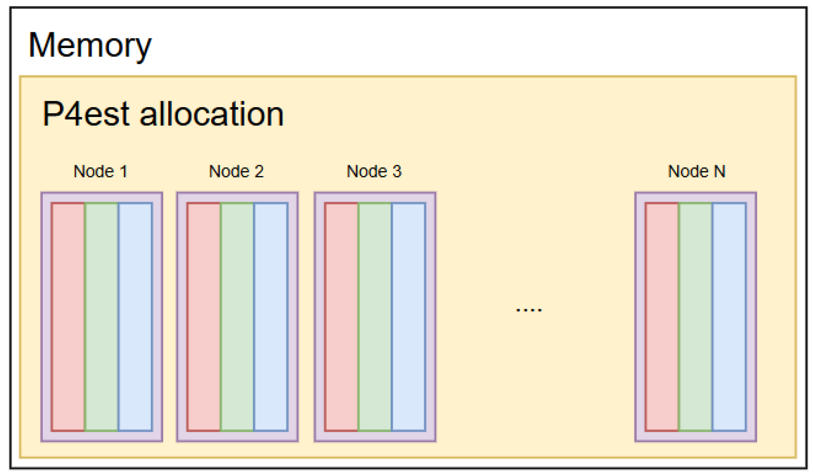
Referring to Figure 2, in order to interface with user applications, p4est allocates a user-specified block size in the memory for every node (purple block in the figure). In grid block-based AMR, the allocated block size would store the grid block’s flow field. Thus, for a grid block consisting of N cells, it would consist of N number of flow-field properties, namely, G p = [ ρ , u, v, w, T, k, ω ] and G s = [ μ , p, T , u , v , w , k , ω ] (red and green blocks in the figure). G p is labeled the primary flow properties while G s are labeled the secondary flow properties. The latter is derivable from the former. The allocated block also stores an N number metric terms, namely, the MUSCL limiters, G l = [ ψ 1 , ψ 2 , ψ 3 , ψ 4 , ψ 5 ] (blue block in the figure). The allocated blocks are automatically managed by the library; access to and manipulation of these blocks is performed through callback functions provided by the user to the p4est subroutines.
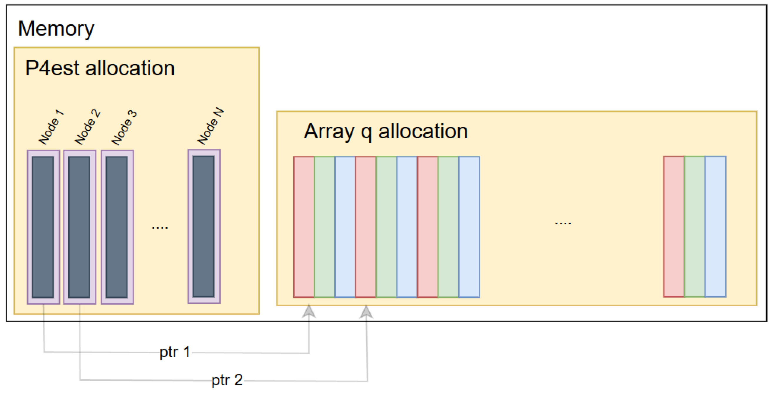
In this paper, we propose a decoupled interfacing approach with the p4est library, as illustrated in Figure 3. The flow-field groups, G p , G s , and G l , are stored separately in another data structure such as an allocated array, q. Instead of storing flow properties directly, each node in p4est is allocated a block storing a data structure group that contains an address pointer, ptr, pointing to the address of the blocks, G p , G s and G l in the array q, and the MPI rank number to which the node belongs. This group is represented in the figure by a black block.
To understand the logic and benefits of this approach, we examine the role of p4est throughout the AMR process, namely the balanced grid adaptation process and the load balancing process. In the balanced grid adaptation process, the off-body Cartesian grid is used for refinement or coarsening according to a flow-field property evaluated by a sensor function. The grid refinement and coarsening are then applied while maintaining a maximum refinement level difference of one between any two adjacent nodes. In p4est, this is achieved through the following sequence of forest adaptation subroutine calls: (1) p4est_refine, (2) p4est_balance, (3) p4est_coarsen, and (4) p4est_balance. The refinement and coarsening calls apply an injection and an averaging operation to initialize the flow-field properties of the created child or parent grid blocks’ cells. For a given flow-field property, ϕ , from child cells j to parent cell i, the injection operation is simply as follows:
ϕ j = ϕ i
Whereas during coarsening from child cells j to the parent cell i the averaging operation is defined as follows:
ϕ i = j = 1 J ϕ j V j V i
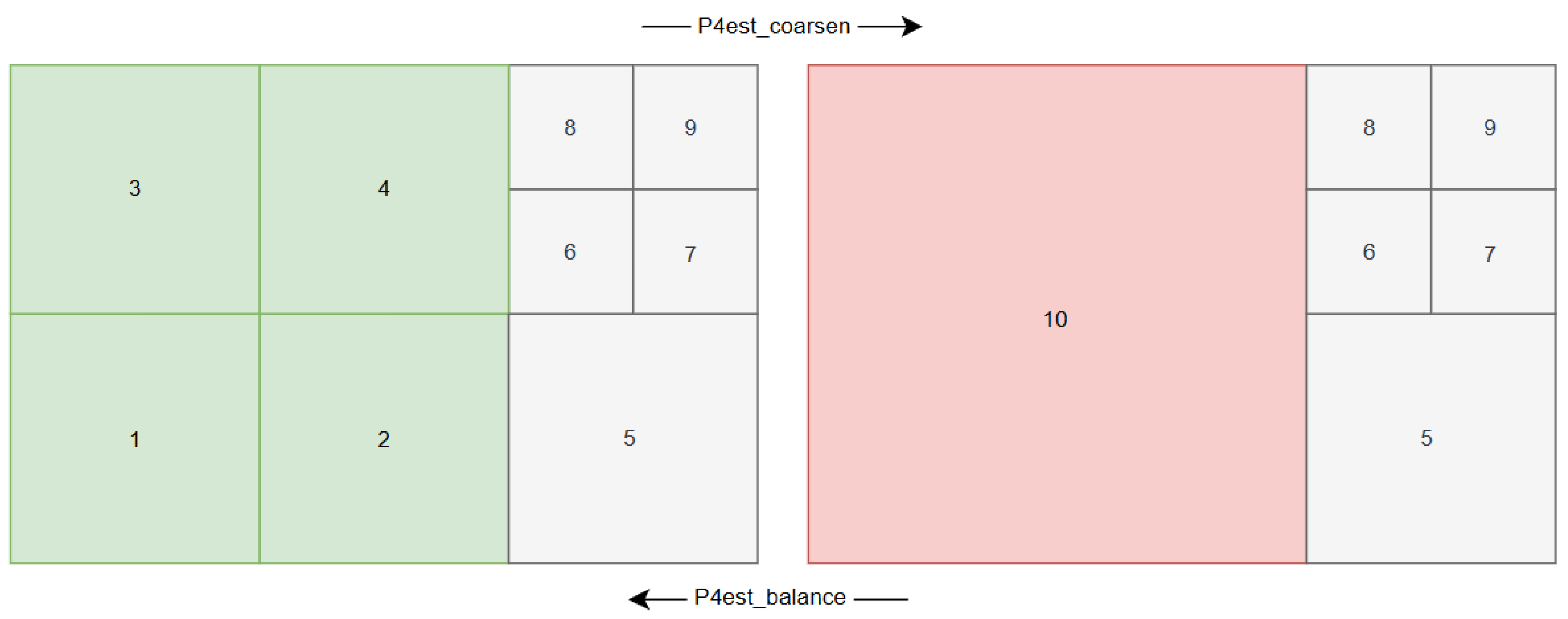
As the p4est_coarsen subroutine does not enforce the 2:1 balance condition, the subsequent p4est_balance call is required. This additional balancing step effectively reverts much of the coarsening where its resultant nodes violated the balance condition, thus resulting in a loss of resolution, delay in convergence and wasted computational effort. To illustrate this behavior, a collection of nodes labeled 1 to 9 is shown in Figure 4. Nodes 1 to 4 are marked for coarsening (green). Calling p4est_coarsen replaces those nodes with node 10. Node 10, holding a given flow property, ϕ , as ϕ 10 = 1 / 4 j = 1 4 ϕ j , violates the 2:1 balance (marked red) with respect to the adjacent nodes 6 and 8. To restore the balance, it is refined as part of the subsequent subroutine call p4est_balance where the resultant, reverted nodes 1 to 4 now hold the flow property as ϕ 10 resulting in a finite error of ϕ j ϕ 10 in a given node j = 1 to 4. In contrast, in the proposed data structure approach, the p4est_coarsen is called without any grid initialization process. As the flow field is separately stored, the flow-field data of the child nodes persist. When the p4est_balance clears the violating coarsened nodes, the flow-field data are simply reassigned back to the regenerated child nodes. As a result, the computational overhead and loss of resolution are completely avoided. If the resultant coarsened node persists after the balance call, the masked nodes’ flow-field data are freed.
The second important function in p4est is load balancing. During the solution process, at the end of a given iteration n, an AMR is invoked. The resultant Cartesian grid adaptation introduces workload imbalances across the MPI ranks. To redistribute the load, p4est employs the p4est_partition subroutine, which redistributes the nodes and their associated user data across the MPI ranks, thereby restoring the balance. The p4est_partition subroutine fully transfers the p4est user-allocated data. In the classic p4est interfacing approach, these data groups correspond to G l , G p , and G s which are associated with the N cells being migrated across M nodes. However, migrating all of these data groups is unnecessary. In a density-based finite volume solver, the non-gradient terms in the data group G s can be recomputed from G p (for example, pressure can be obtained from density and temperature using the equation of state). Moreover, due to the structure of the solver cycle, the gradient terms in G s and the limiter terms in G l are obsolete during the data migration stage, as they correspond to iteration n 1 , in contrast to G p , which corresponds to iteration n. Consequently, migrating these obsolete and reproducible terms serves no purpose, as they are simply overwritten when the gradient and limiter solver subroutines are called during the next solution cycle. In the proposed data structure, instead of transferring the full data groups, only the address pointer and the source MPI rank are migrated. Using this information, a set of distributed MPI send/receive buffers is constructed, through which only the data group G p is communicated. The groups G s and G l are then reconstructed from G p later in the solver cycle using the gradient and limiter subroutines. Although the load-balancing communication stage is now split into two phases, the overall volume of communicated data is drastically reduced. This significantly lowers the communication time overhead and, consequently, the total solver runtime.

3.3. Parallel Overset Grid Reassembly Method

As the Cartesian grid adapts to the flow field, new grid blocks are introduced while others are replaced, changing its topology. As the load balancing call is made, the Cartesian grid connectivity information also changes. The current donor–receiver pairs and the interpolation coefficients are thus invalidated. To remedy this, a grid assembly step is required after every grid adaptation process, in which the receiver and donor pairs are re-established and the interpolation coefficients are recomputed between the newly adapted and repartitioned Cartesian grid and the body-conforming grid. Although a master-core approach for handling the entire reassembly process may seem attractive, it significantly reduces parallel scaling performance and can lead to substantial memory requirements. In a master–slave approach, grid partitions across all MPI ranks communicate their receiver cells to a master MPI rank. This master rank, which holds the full body-conforming grid information, performs the spatial search to identify donor–receiver cell pairs and computes the interpolation coefficients. It then sends the results back to the respective MPI ranks. Consequently, a parallel distributed overset grid reassembly process must be considered.
Works by [42,43] showcased good scaling performance in the overset grid assembly process by using bounding boxes to represent the different overset grid partitions and establish communication between them. In this paper, we follow the same approach while also exploiting the p4est octree structure. The Cartesian and body-conforming grids partitioned across a set of MPI ranks are each represented by a bounding box with extreme coordinates x m i n and x m a x , along with their receiver cell layer (if any). The receiver-cell bounding boxes are then broadcast to all MPI ranks, where bounding-box intersection tests are performed. For a given partition A and B, the intersection test is given by
x A , max x B , min x A , min x B , max
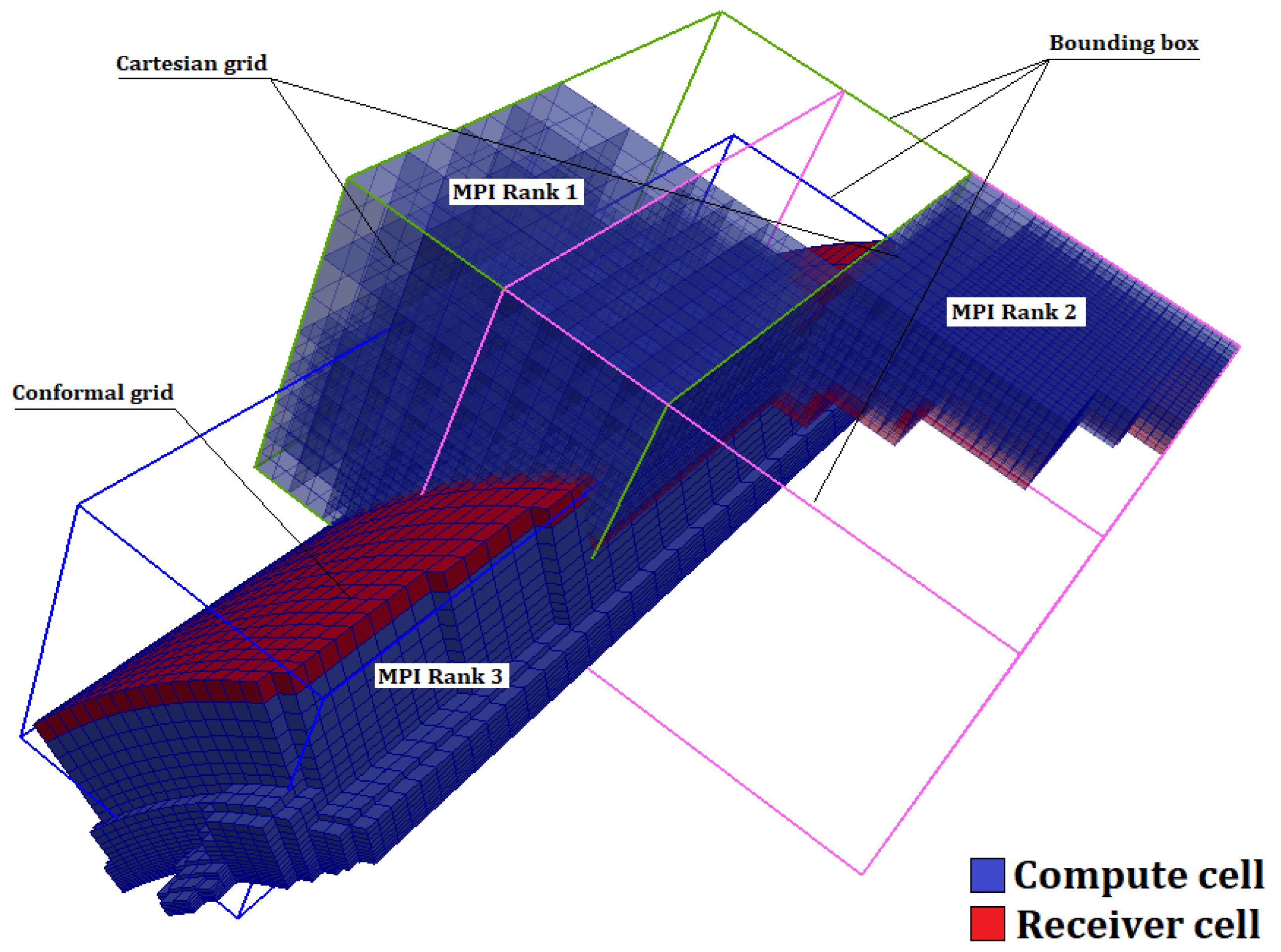
Figure 5 shows a body-conforming grid and two Cartesian grid partitions, each held by a separate MPI rank. The receiver cells of the body-conforming grid partition are represented by a bounding box outlined in blue. The Cartesian grid partitions are represented by bounding boxes outlined in green and purple. The bounding box of the body-conforming grid partition’s receiver cells intersects those of the Cartesian grid partitions. MPI ranks that detect such intersections share their receiver cell geometry data with the intersecting ranks. In the figure, MPI rank 3 sends its body-conforming grid receiver cell geometry data to MPI ranks 1 and 2.
To efficiently establish the donor–receiver cell pairs, the submitted receiver cells are spatially queried using their bounding box coordinates, x m i n , x m a x and centroids x c against a digital tree representation of the grid partition in question.
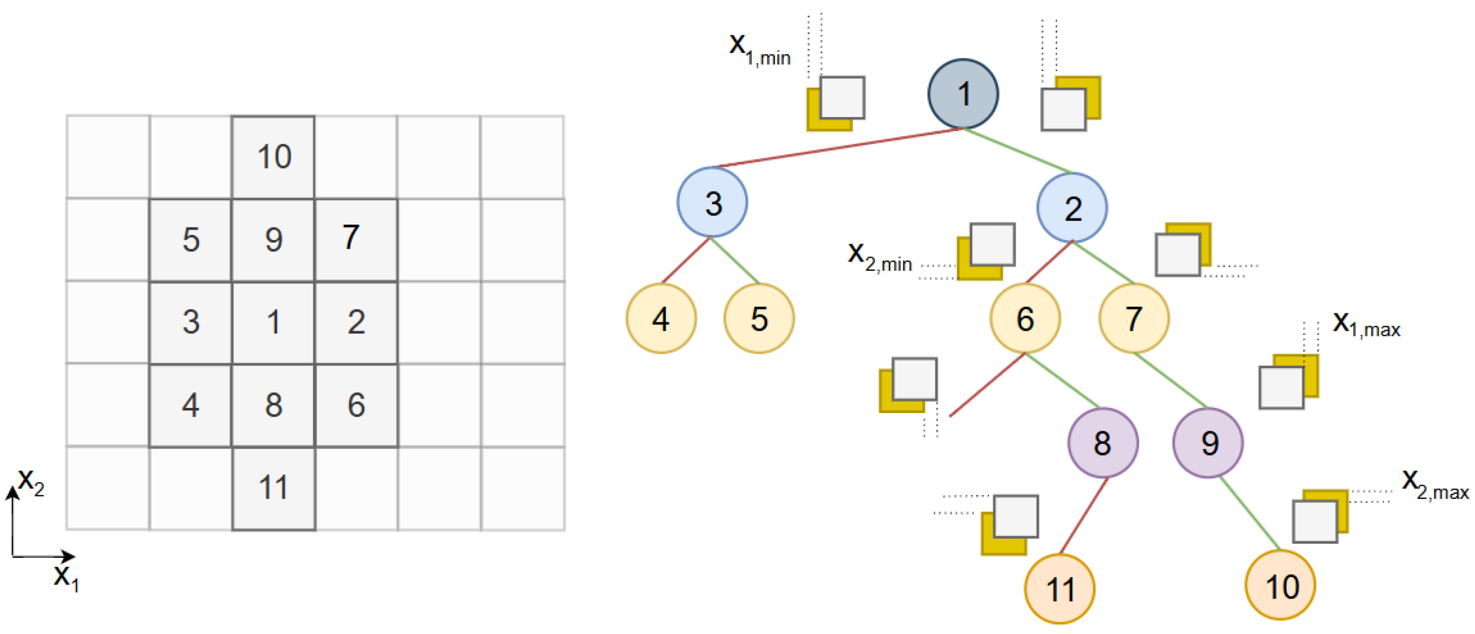
An Alternating Digital Tree (ADT) is used to represent and spatially query the body-conforming grid cells. Referring to Figure 6, the ADT is a binary tree consisting of nodes, represented by circles, which are sorted at multiple levels, each represented by a different color. Each node represents a body-conforming grid cell. A given node at a given level has two child nodes to which it branches when navigating to the next level and a parent node from which it branches at the previous level. The child nodes are sorted to the right or left branch with respect to their parent according to the i t h component of the relative bounding box maximum x i , m a x or minimum coordinate x i , m i n , where the left branch corresponds to a “less than” sort and the right branch corresponds to a “greater than” sort. For example, in the figure, node 2 is placed at the 2nd level. It is sorted from its parent (node 1) through the right branch because its bounding box x 1 , min is greater than that of its parent. The child nodes 6 and 7 are inserted to the left and right of node 2, respectively, due to their x 2 , min being less than and greater than that of node 2. Nodes are inserted according to the aforementioned sorting rule until a vacant position is found. Since the body-conforming grid is pre-partitioned, the ADT can be constructed at the beginning of the solution process and stored in memory throughout the solver computation.
To query a cell using its bounding box for body-conforming grid cells potentially intersecting with it, a search begins at the root node of the ADT. At each node, a bounding-box intersection test (Equation (12)) is performed between the search cell and the node’s bounding box. If the test fails (no intersection), the corresponding coordinate component of the search cell’s bounding box is compared to the splitting (sorting) value at the current level. Depending on the result, one branch (left or right) is entirely pruned, eliminating the search in that half-space. This pruning is what yields the method’s efficiency. If the bounding boxes intersect, the current node is added to a list of candidate donors, and the search recurses down both branches to the next level. Once the traversal of the ADT is complete, the candidate whose centroid is closest to the search cell’s centroid is selected as the donor cell. Its immediate neighboring cells are typically included as well to complete the interpolation stencil.
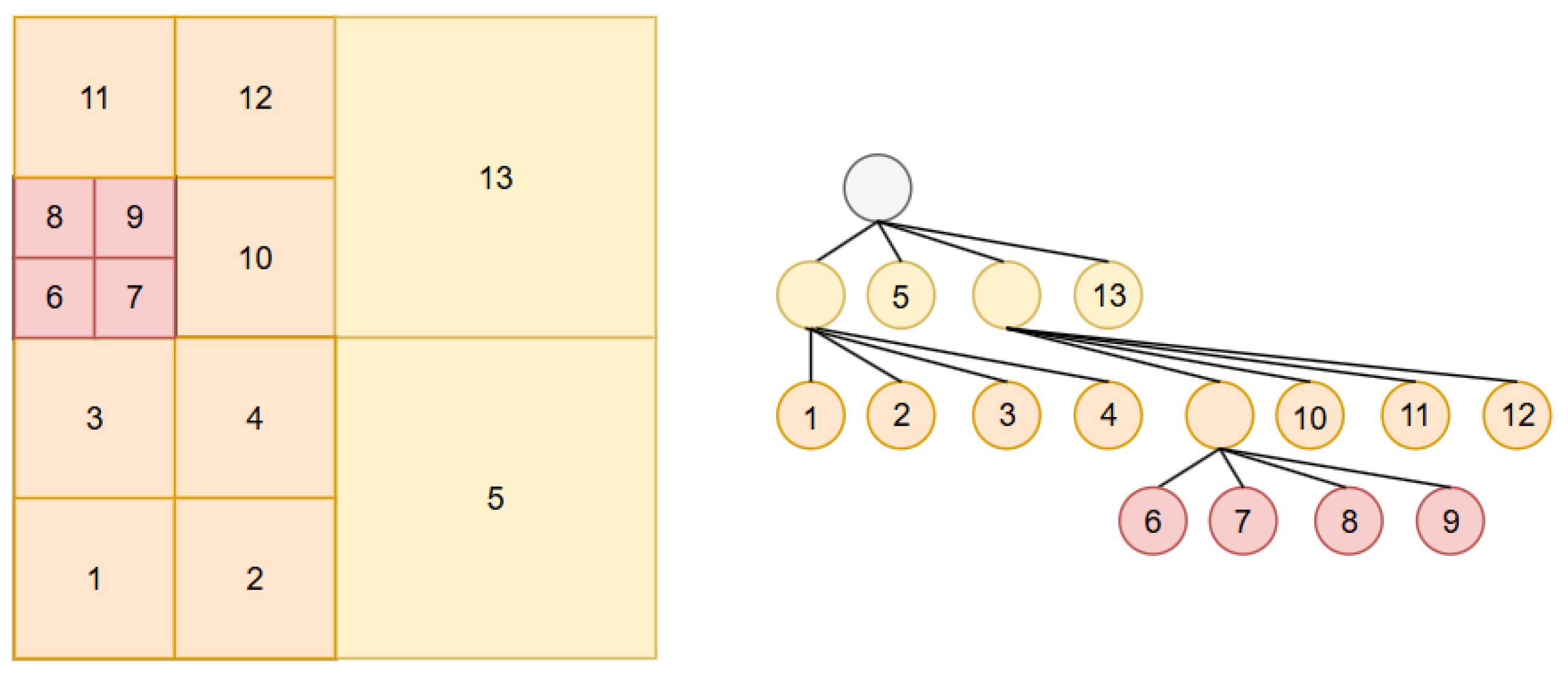
The Cartesian grid—governed by the p4est octree forest—can be efficiently represented and spatially queried for any given point in space using the already available octree structure. An example of this is shown in Figure 7 where a two-dimensional Cartesian grid sample is represented by the degenerate two-dimensional case of the octree, namely the quadtree. The different refinement levels are indicated using different colors. For a receiver cell with centroid coordinates x c belonging to the body-conforming grid, Cartesian grid query for a candidate donor starts by quantizing the coordinates to L-bit integers according to the highest refinement level L of the octree. In a three-dimensional setting, these bits are then interleaved to form a single 3 × L -bit Morton code. Traversal is performed by repeatedly extracting the lowest 3 bits of the Morton code (which give the child index) and then right-shifting the code by 3 bits until a childless node is reached. This corresponds to the target grid block. From there, the structured grid relation can be used to find the donor pair.
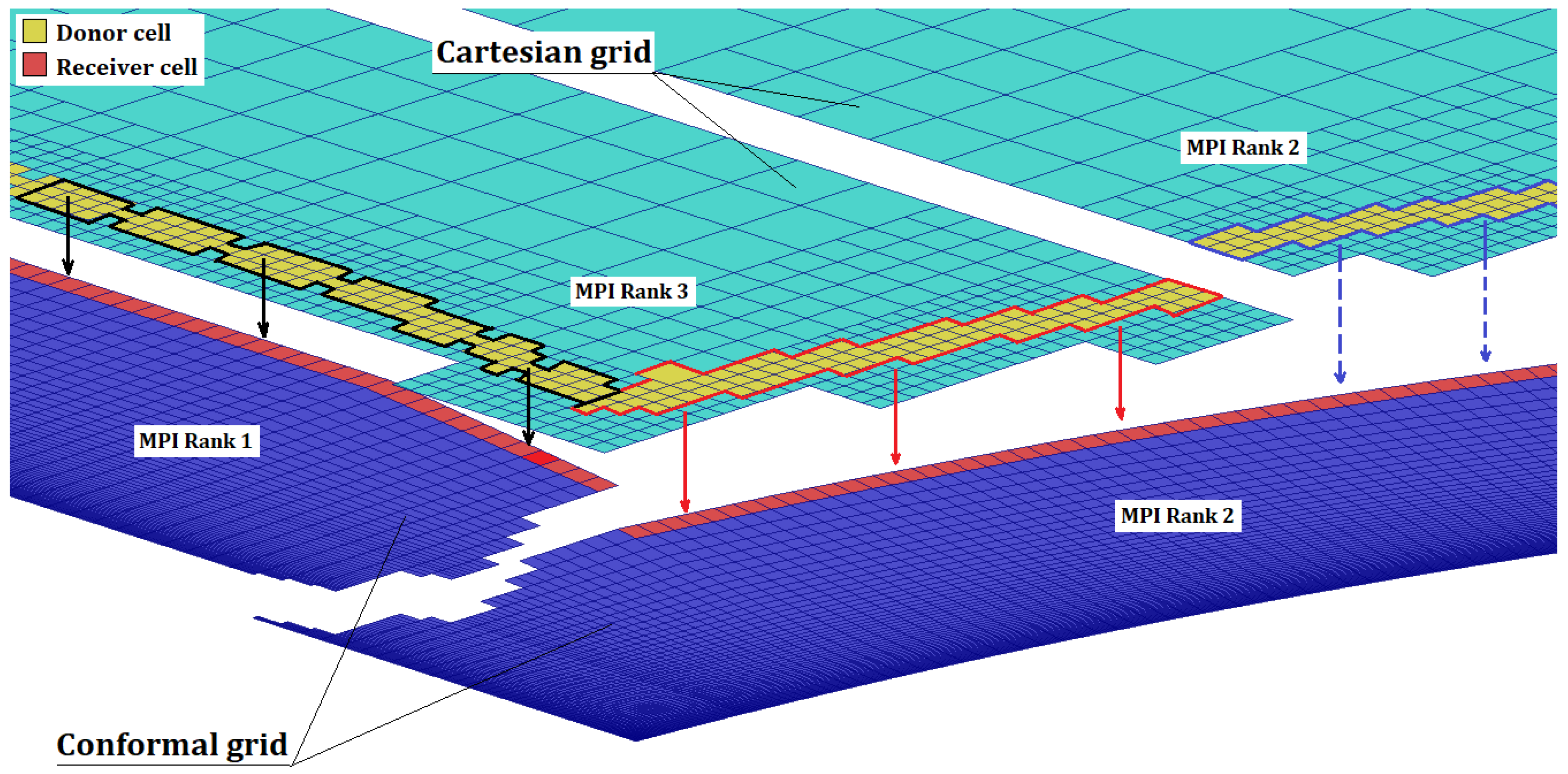
Using the obtained receiver–donor pairs, the interpolation communication tables are established. Communication in which MPI ranks exchange donor-cell flow-field values with the MPI ranks holding the corresponding receiver cells is referred to as inter-grid communication. Figure 8 shows an example of inter-grid communication. In the figure, two partitions of each of an overlaying body-conforming grid (blue) and a Cartesian grid (cyan) are shown in an isometric view. Each partition is assigned to an MPI rank. Since the MPI rank 3 Cartesian grid partition overlays the body-conforming grid partitions of MPI ranks 1 and 2, it communicates the donor cells (yellow) to each of these MPI ranks. The donor cells outlined in black are communicated to MPI rank 1, while the donor cells outlined in red are communicated to MPI rank 2. The arrows show the data transfer direction. Since MPI rank 2 owns two overlaying Cartesian and conformal partitions, a dummy communication occurs between them, as indicated by the dashed blue arrows. The receiver cells, marked in red, are then reconstructed using the donor cell data. This communication occurs prior to every interpolation update during the solver iterations.

4. Benchmark Studies

To validate the solver, we consider two benchmark three-dimensional flow problems: a steady compressible flow over a semi-infinite blunt-nose cylinder and a transient compressible flow diffraction over a sphere. The solver is run on a dual-socket compute node of an HPC system. The node is equipped with two AMD EPYC 7742 processors (2.25 GHz base frequency), providing a total of 128 cores.

4.1. Case I: Steady Flow over a Semi-Infinite Cylinder with a Blunt Nose

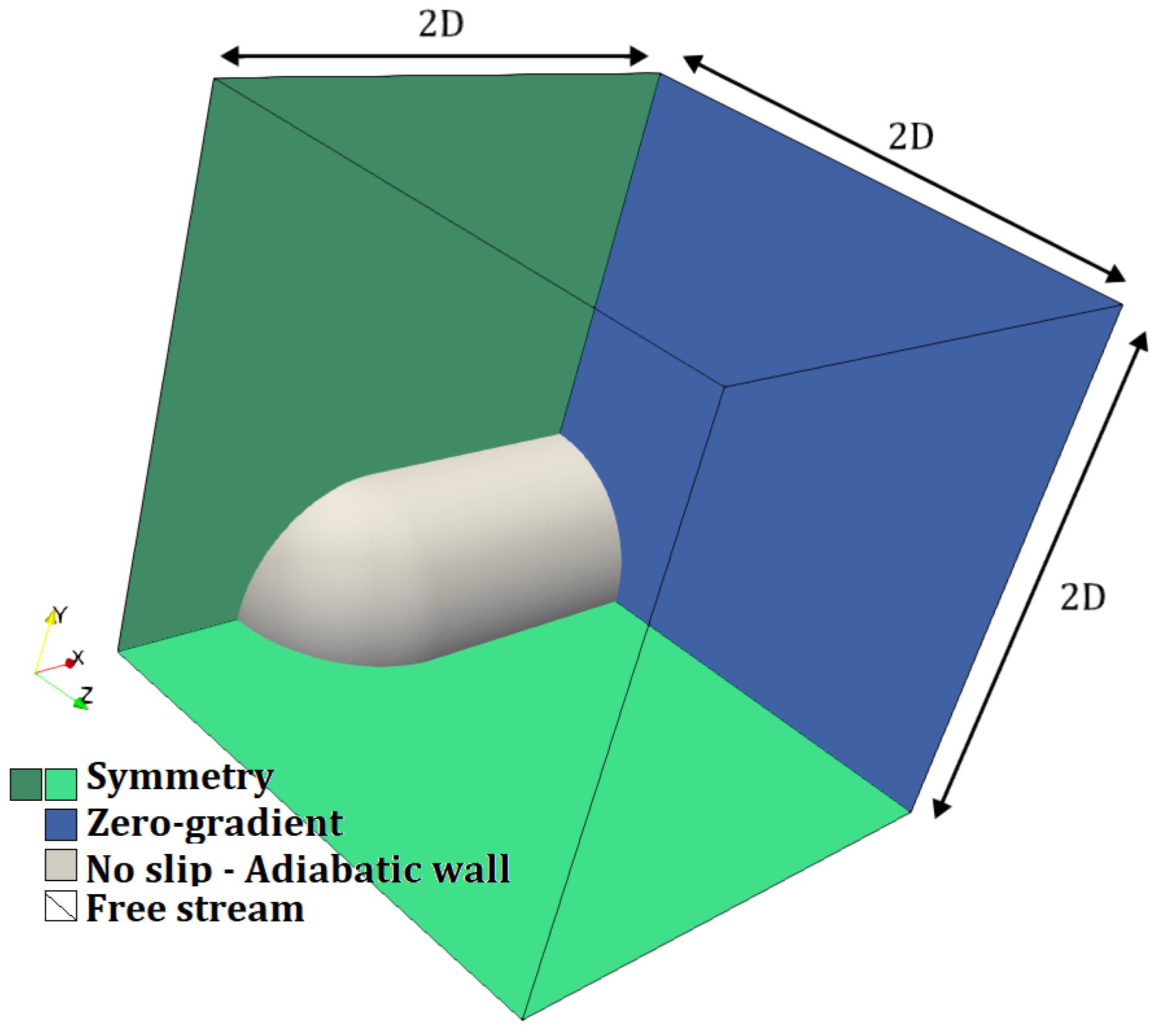
To assess both the accuracy and parallel performance of the solver, as well as the efficiency of its individual interpolation and iteration components, the experimental study by Sahoo et al. [44] is considered. The flow-field free stream properties are presented in Table 1. Although the problem’s axisymmetric nature allows for two-dimensional modeling, the primary objective here is to demonstrate the solver’s performance in a three-dimensional setting, which is inherently more computationally demanding. Therefore, the flow is modeled using a quarter of the entire computational domain. The domain and the applied boundary conditions are shown in Figure 9.
The Cartesian grid is generated with a 3 × 3 × 3 forest where each node represents 2 × 2 × 2 grid blocks. The maximum refinement level is set to 5, with the Mach gradient taken as the refinement criterion with threshold range values of Q l o w e r = 0.185 and Q u p p e r = 0.218 . The selected threshold values are such that the bow shock is fully engulfed by the highest allowable refinement level. Therefore further restricting threshold values does not affect the solution. The spacing of the first layer of the body-conforming grid from the wall corresponds to y + = 5 . Grid adaptation is successively applied as the solution approaches steady state. The convergence criterion is set to 0.01% in cumulative residual relative error. The coefficient of pressure is evaluated over the surface of the blunt nose, where it is given by
C p = 2 γ M 2 p p 1
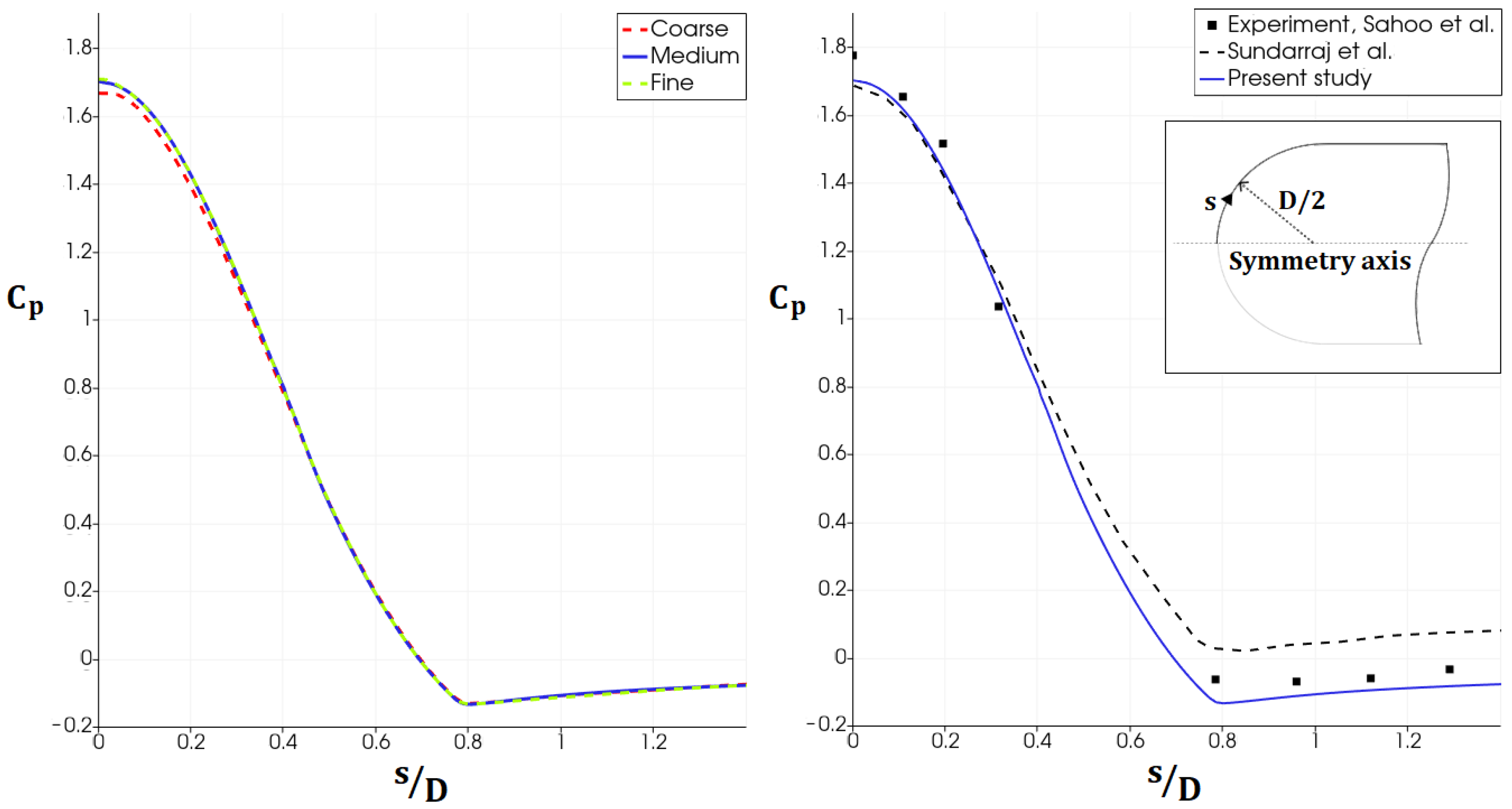
This selected medium grid resolution is found to be adequate for resolving the flow field when compared with a coarse and fine grid whose maximum refinement levels are 4 and 6 as shown in the Cp plots in Figure 10 (left). At steady state, the selected medium adapted overset grid contains 1,419,996 cells, while the coarse and fine grids contain 334,627 and 3,697,852 cells.
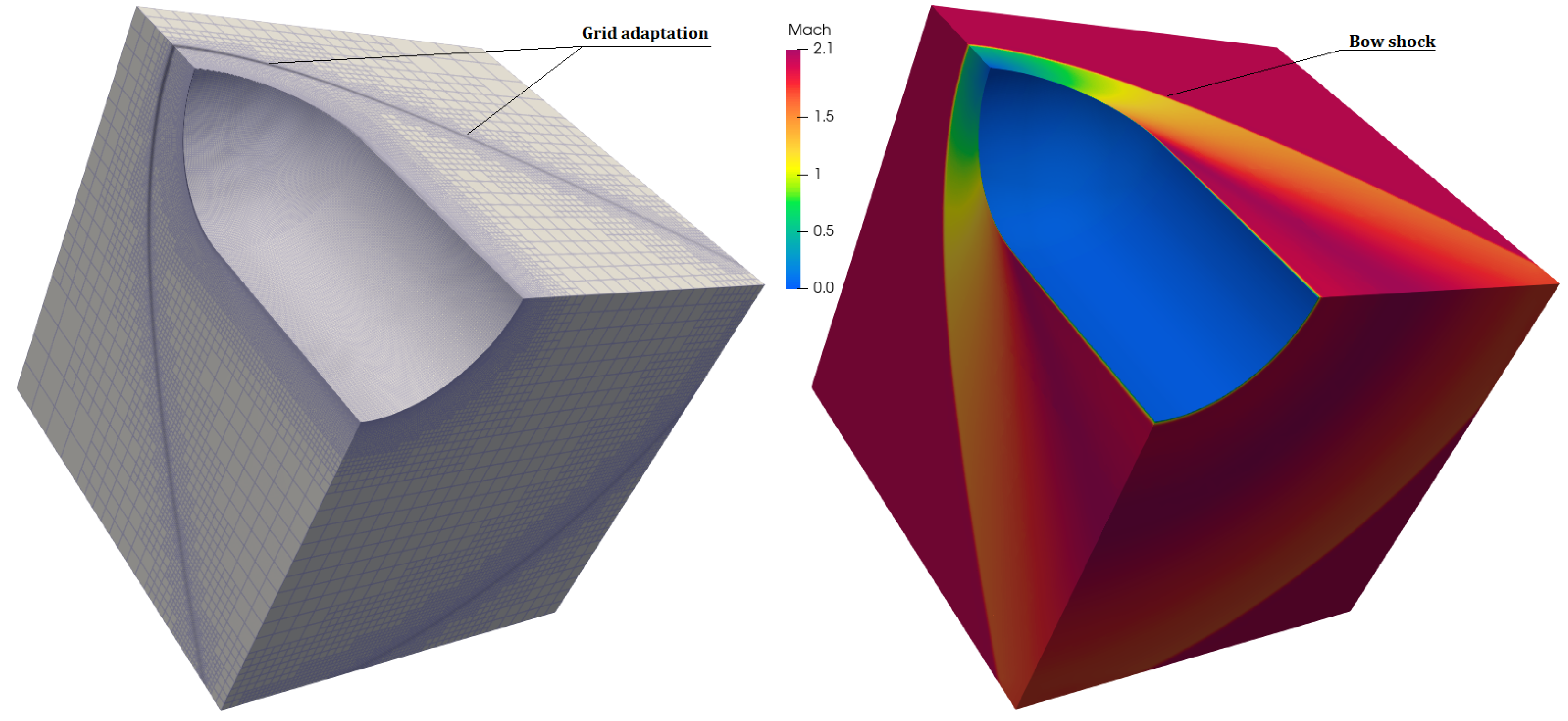
Figure 10 (right) shows the C p distribution along the blunt body surface. The obtained numerical result is in good agreement with the experimental data, except at the stagnation point ( s / D = 0 ) and the tip base ( s / D > 0.8 ), where it is slightly under-predicted. Nonetheless, the obtained distribution is in better agreement with the experimental data compared to the numerical results obtained by Sundarraj et al. [45] using Software Cradle’s CFD solver, scFLOW V2020. Figure 11 illustrates the resultant grid adaptation and the corresponding numerical schlieren image upon reaching the steady-state solution. The obtained Mach contours are also shown. As seen in the figure, the grid properly adapts along the bow shock, providing a starker resolution of the discontinuity.
To investigate the solver’s parallel performance, its strong scaling behavior is considered. The resultant overset grid at steady state is kept constant while the number of MPI ranks is increased by a factor of two at each step. Of the 1,419,996 cells contained by overset grid at steady state, 34,970 are marked as receiver cells. The wall-clock execution time is recorded for 100 iterations, covering both the interpolation segment within the solver and the complete iteration cycle. The speed-up factor, S f and parallel efficiency η at a given number of MPI ranks, N, are defined as follows.
S f = T 1 T N
η , % = S f / N × 100
where T 1 and T N are the times taken for the given process to complete with 1 and N MPI ranks, respectively. Additionally, in order to establish a point of reference with respect to the HPC system and the solver’s base parallel performance, the solver is run in a single-grid mode where the case is solved over the body-conforming grid only. In this case, the body-conforming grid’s outer boundary is extended to reach the far-field and achieving the same cell count as the overset grid. The obtained S f and η values are presented in Figure 12.
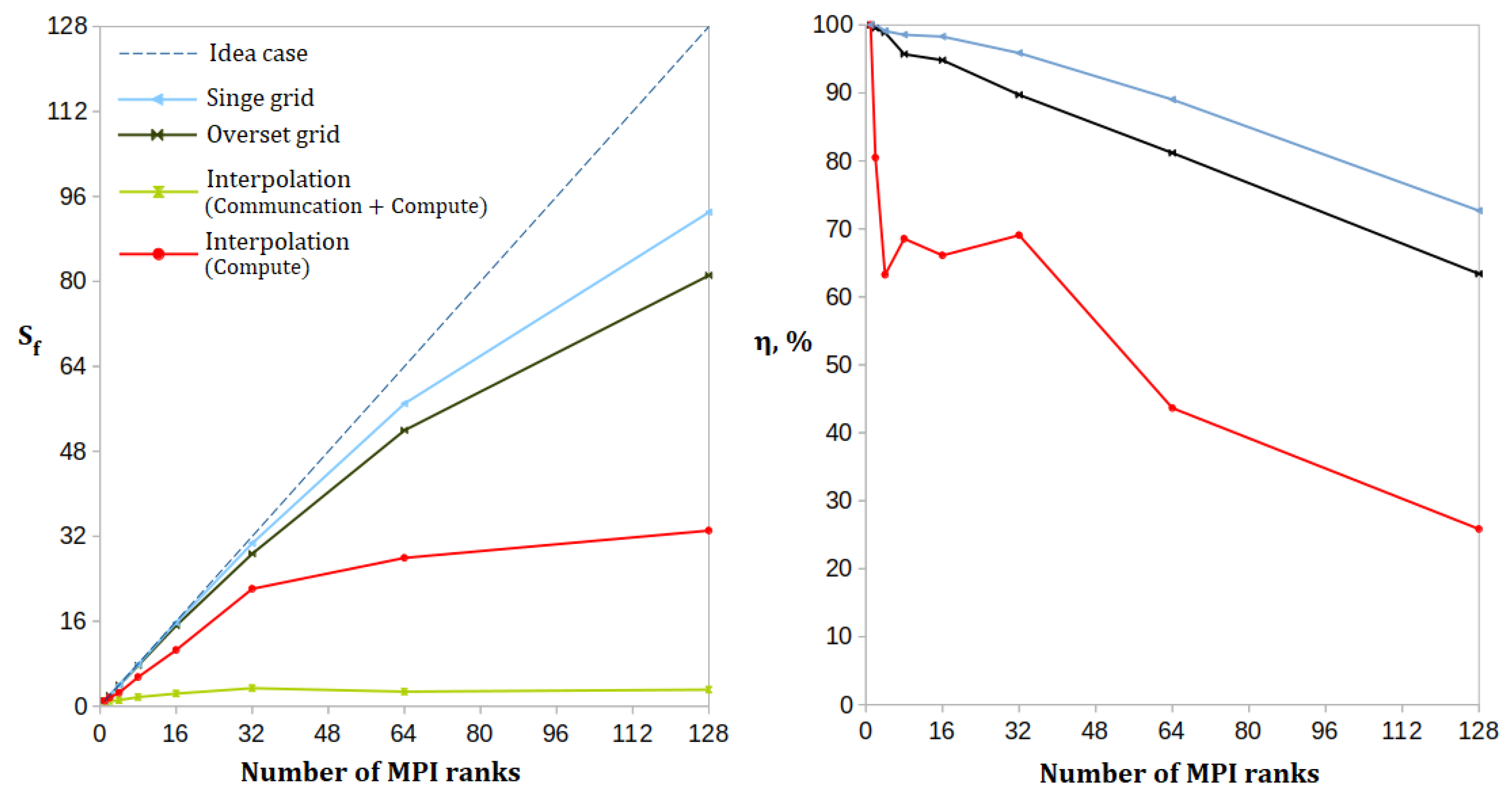
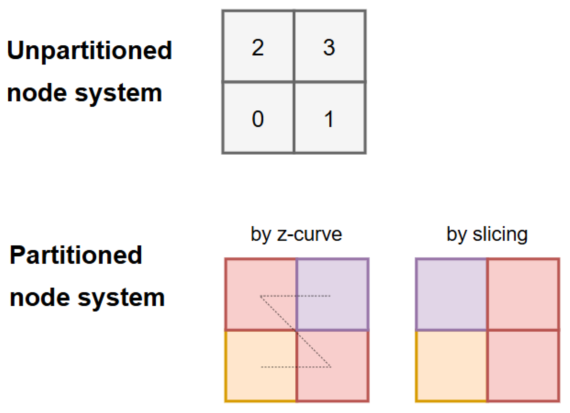
The present solver in overset grid mode (black line plot) shows strong scaling up to 32 MPI ranks, where the parallel efficiency corresponds to 89.7 % . Then, a drop in efficiency takes place at an MPI rank count of 64, with the efficiency decreasing to 80 % . At 128 MPI ranks, the parallel efficiency drops to 65 % . When compared with the single grid, the present solver in overset grid mode exhibits a reduced parallel performance of up to 7 % at 128 MPI ranks. This difference is attributed to the distinct grid decomposition methods in the two modes. Figure 13 shows a system consisting of 4 nodes. In a typical partitioning approach, the nodes are distributed among 3 MPI ranks (different colors) by horizontal and vertical cuts. In the Z-curve case, the partitioning follows the space-filling curve. This leads to MPI ranks with larger interface surfaces bordering neighboring ranks. As seen for the red rank, four faces border other ranks, in contrast to only two faces in the typical partitioning approach. Nonetheless, the solver scales relatively well with the increased number of MPI ranks. The interpolation component of the present solver is plotted in the figure with a yellow line. This component consists of computation and communication segments. Due to the small number of donor–receiver cells, the communication segment dominates the scaling performance, while the computation segment’s scaling contribution is comparably small. As non-blocking communication mitigates the interpolation communication penalty, its impact on the solver is limited. Thus, the computation segment alone (red line plot) provides a clearer metric for interpolation performance. The interpolation computation segment shows steady scaling performance with a parallel efficiency of 70 % at MPI rank counts up to 32. In contrast to the solver’s overall scaling performance, the interpolation computation segment is weaker. This is anticipated, as the donor–receiver cell pairs are not equally distributed among the overset grid partitions. At MPI rank counts of 64 and 128, the parallel efficiency drops to 44 % and 30 % , respectively. This is due to the very small number of donor–receiver cell pairs in each MPI rank. Considering that the interpolation component constitutes from 0.2 % (1 MPI rank) to 5.11 % (128 MPI ranks) of the solver iteration time, its impact on the present solver’s overall scaling performance is small. When compared with the master–slave approach from [30], the proposed approach provides a 50 % increase in the solver’s overall parallel efficiency at 32 MPI ranks relative to the previously reported value.

4.2. Case II: Transient Flow on a Sphere

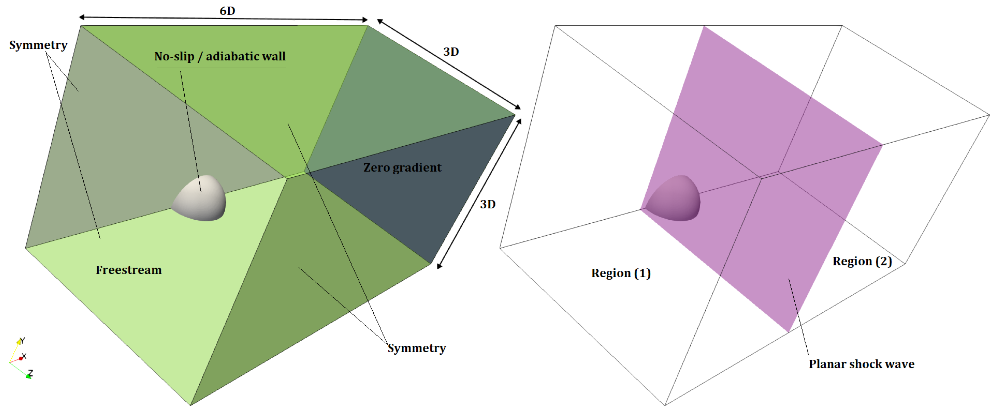
The shock diffraction problem, originally studied experimentally by Bryson and Gross [46], is used as a benchmark to evaluate the dynamic parallel performance of the developed solver. The test case consists of a planar normal shock wave propagating towards a sphere of diameter D in quiescent air. Figure 14 shows the computational domain, the applied boundary conditions, and the two flow-field regions separated by the planar shock wave. The flow field in region (1) is stationary, while region (2) has a finite x-axis aligned velocity with post-shock properties. The planar shock propagates at Mach number 2.89 as initially seen by region (1)’s flow field. The flow-field properties in the two regions are given in Table 2. The flow is laminar, with the Reynolds number defined as R e = D V ν and set to 7800. Both the kinematic viscosity ν and the velocity V are based on the post-shock flow properties. The dynamic viscosity is held constant, independent of temperature. Air is used as the working fluid. Accordingly, the gas constant, specific heat capacity at constant pressure, and specific heat ratio are set to R = 287.2 J/(kg·K), c p = 1005.2 J/(kg·K), and γ = 1.4 , respectively.
The computational domain is discretized using a Cartesian grid generated from an octree forest of 10 × 5 × 5 base nodes, with each node containing a grid block of 2 × 2 × 2 cells. During the solution procedure, the adaptive mesh refinement routine is invoked every 25 iterations of the flow solver. This adaptation frequency, combined with the selected block resolution, was found to adequately resolve and track the incident discontinuity and all subsequent flow features within block grids of the highest refinement level at all times as they propagate while maintaining a high computational load on the solver. The maximum refinement level is set to 5. The density gradient is taken as the refinement criterion with the threshold range values of Q l o w e r = 0.6 and Q u p p e r = 0.625 . A body-conforming grid is employed near the sphere surface, with the first cell spacing corresponding to y + 2.5 . This grid extends outward from the sphere surface by 2.5 D . This arrangement ensures that near-body shock phenomena are primarily captured by the Cartesian grid, while the boundary layer is adequately resolved by the body-conforming grid. With the stated settings, the initial overset grid system consists of 3,241,936 cells, of which 54,294 are receiver cells. Denoting the non-dimensional time, as t ¯ (normalized by D / V ), the solution is obtained at CFL number of 0.7. This corresponds to a global non-dimensional timestep, Δ t ¯ range of 9.2 × 10 5 to 1.5 × 10 4 at different iterations.
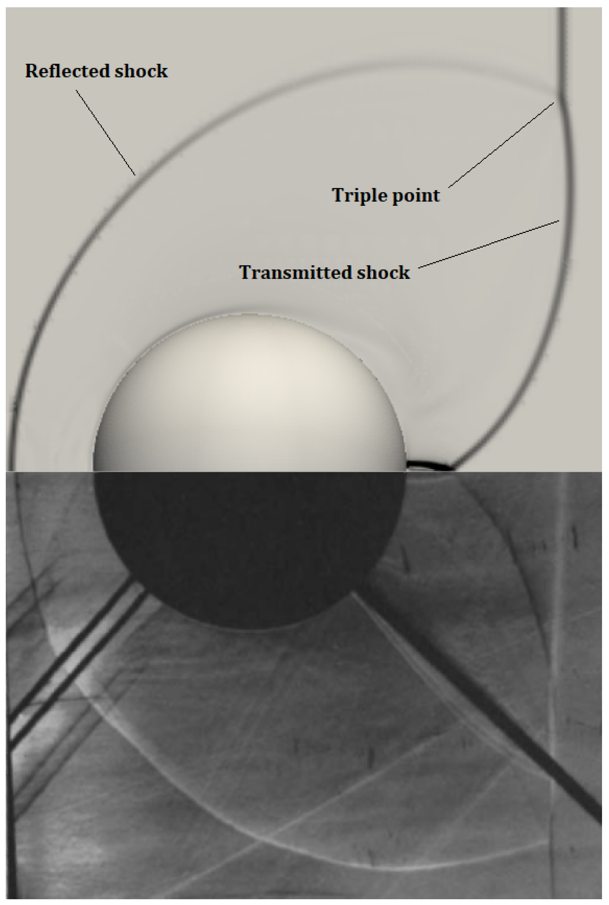
To validate the solver’s numerical setup, the computed numerical schlieren image of the flow field is compared with the experimental results reported by Bryson and Gross [46], as shown in Figure 15. The computed locations of the reflected shock, triple point, and transmitted shock show good agreement with the experimental data. The standoff distance of the reflected shock is slightly different from the experimentally reported value. This discrepancy is likely attributable to imaging artifacts, as evidenced by several irregular deformations visible in the experimental image.
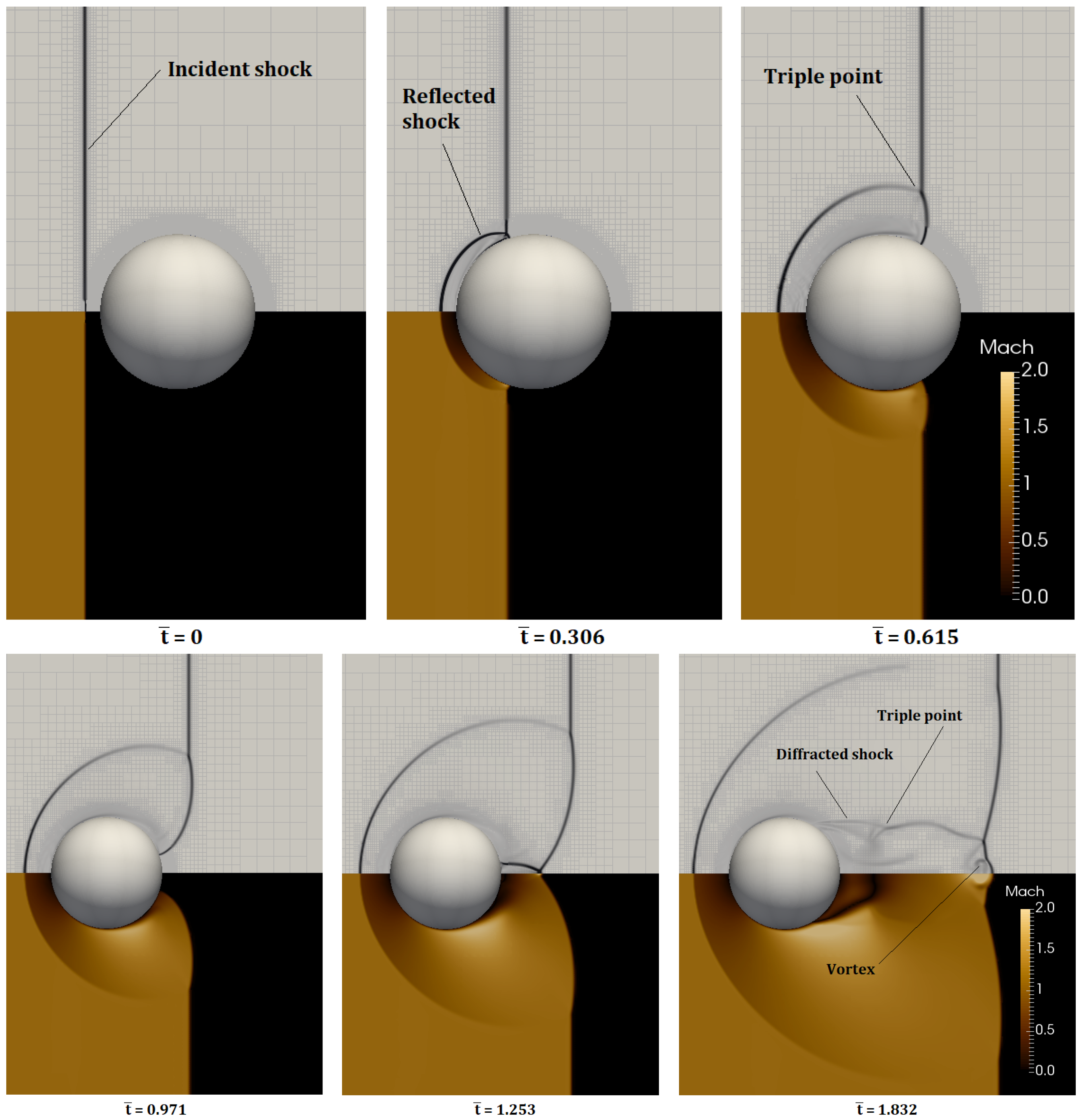
The numerical schlieren images and Mach number contours of the flow field are shown in Figure 16 at different t ¯ values. At t ¯ = 0 , the incident planar shock is at 0.6 D from the sphere centroid. As the shock intercepts the sphere surface, a reflected shock emanates from it ( t ¯ = 0.307 ). A triple point forms at the intersection of the reflected and incident shocks ( t ¯ = 0.615 ). As the incident shock propagates downstream, the diffracted shock and its triple point emerge over the sphere wake ( t ¯ = 1.832 ). A vortex is also visible. The solver successfully adapts to and tracks the shock structures throughout the solution process, as evidenced by the grid lines of varying resolution in the figures. A slight loss of tracking is observed at t ¯ = 1.832 , where the reflected shock connects to the triple point. This is due to the diminishing density gradient. At t ¯ = 1.832 , the adapted overset grid reaches a total of 3,241,936 cells, up from an initial count of 2,232,704 cells. Due to the large grid size and numerous flow discontinuities driving continuous adaptation, this specific time instance is selected to evaluate the strong scaling and parallel performance of the dynamic AMR.
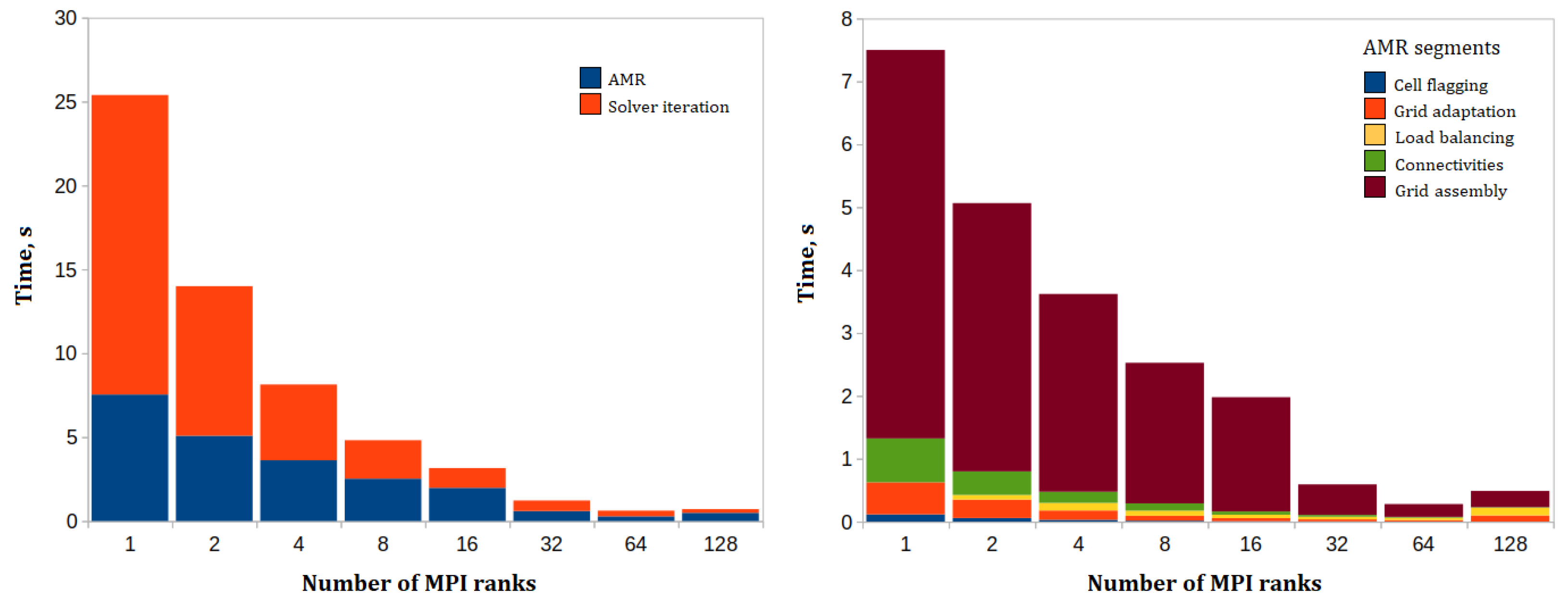
It is noted that an AMR consists of 5 segments that run in order, which are as follows: (1) Cell flagging, where the cells are evaluated by a sensor function then marked for refinement or coarsening against a threshold; (2) grid adaptation, where the grid is adapted according to the placed flags; (3) load balancing, where the grid blocks are migrated to restore the balance and the ghost layers are generated; (4) connectivities, where the cells neighbor connectivities are set and cached; and (5) grid assembly, where the overset grid systems is reconstructed in terms of donor–receiver cells and their interpolation coefficients along with the communication tables.
Figure 17 (left) shows the decomposition of the time taken by an AMR and a single flow solver iteration at different numbers of MPI ranks, while Figure 17 (right) shows the AMR segments’ contribution to the AMR time with respect to those ranks. The time taken by both decreases with increasing MPI rank count. An exception is at 128 ranks, where the AMR time is slightly increased. This increase is attributed to a jump in the number of nodes migrated at 128 ranks compared to the lower rank count, as evidenced by the increase in the time taken by the load balancing segment. The AMR process takes less wall-clock time than, but remains comparable to, a single flow solver iteration for all MPI rank counts. This difference shrinks with increasing MPI rank count. It is worth noting that the AMR process is invoked only once every N flow solver iterations. This translates to a rapidly diminishing computational cost. In this case study, N = 25 . The AMR time equates to 8% of the time taken between each AMR at 128 MPI ranks. When considering the time decomposition over the AMR process segments, the overset grid assembly segment makes up the majority of the AMR time with its lowest contribution percentage being 53%. While the remaining segments scale well with increasing MPI rank count, their contributions to the AMR time are negligible.
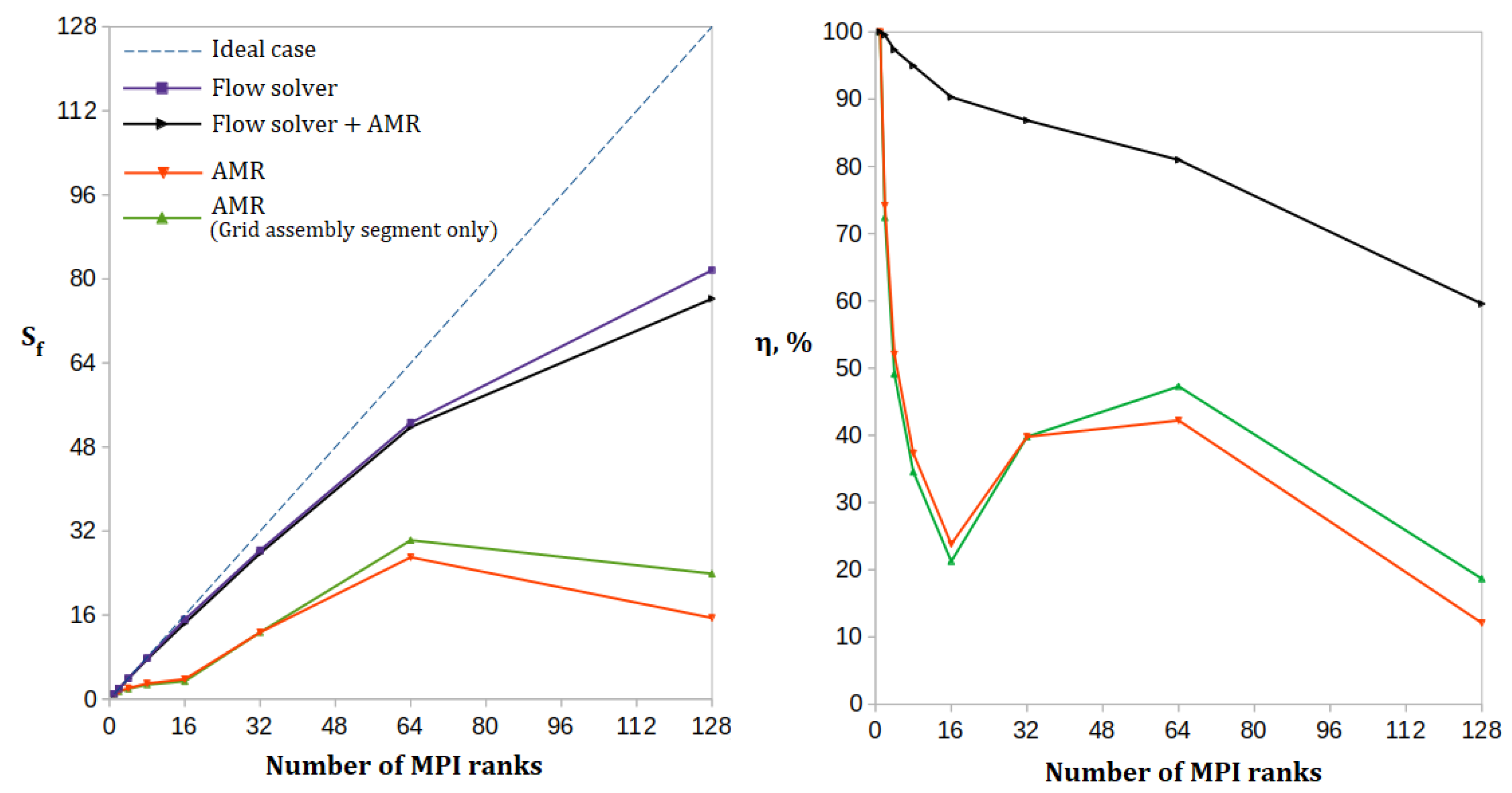
The speed-up factors and parallel efficiencies of the AMR (red line plot) and the flow solver iterations (purple line plot) are shown in Figure 18. The AMR exhibits consistent but relatively weak scaling up to 16 MPI ranks. The scaling performance improves between 16 and 64 ranks, followed by a sharp drop at 128 ranks. To better understand this behavior, the speed-up factor of the overset grid assembly segment—which accounts for the majority of the AMR time—is also plotted (green line plot). The partitioning based on the Cartesian grid’s governing space-filling curve does not assign additional weight to cells overlapping with the body-conforming grid. Consequently, the workload associated with donor and receiver cell queries, as well as the evaluation of interpolation coefficients, is not well balanced across cores. This results in reduced parallel performance in the overset grid assembly segment and, by extension, in the overall AMR process. This imbalance improves at 32 to 64 MPI ranks, leading to better AMR scaling. The performance drop at 128 MPI ranks occurs because the number of receiver cells per rank becomes very small. This causes communication time to dominate and leads to a strong imbalance in the distribution of overlap cells across ranks. Nevertheless, when considering 25 flow solver iterations per AMR cycle, the AMR process has minimal impact on the overall solver scaling performance, as shown by the black line compared to the purple line. The solver maintains a parallel efficiency similar to the steady flow case, demonstrating good scaling for unsteady flow problems with an efficiency of 61% at 128 MPI ranks.
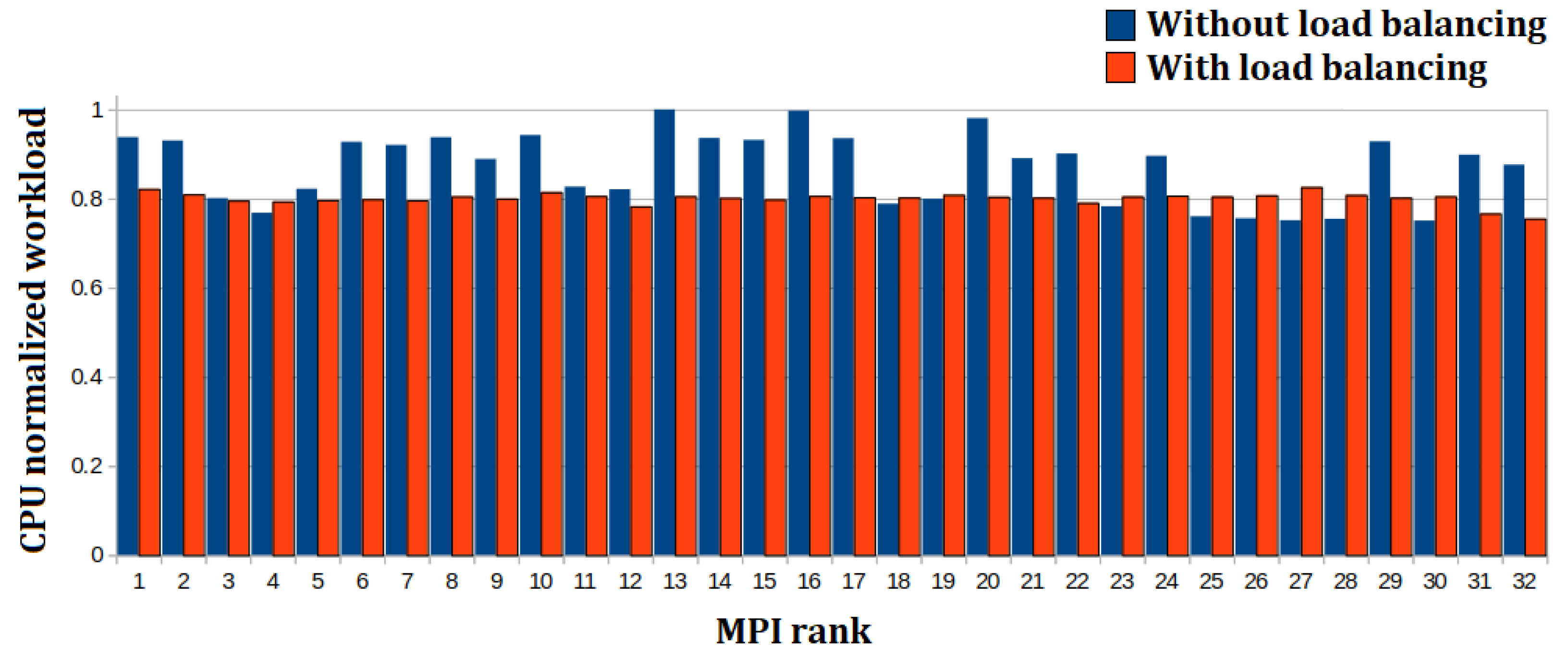
To evaluate the load balancing process, AMR is invoked after 25 iterations, and a subsequent flow solver iteration is then considered. In one case, load balancing is invoked in the AMR, while in the other case it is not applied. The CPU workload time of each MPI rank is measured during the flow solver iteration for both scenarios. These workload times are then normalized by the maximum CPU workload time across all ranks in the respective load-balanced and unbalanced cases. For readability, we consider the case with 32 MPI ranks. The results are presented in Figure 19. The MPI ranks in the load-balanced case exhibit a minimum workload reduction of 17.4% compared to the unbalanced case. In addition, the overall workload distribution is significantly more uniform. Minor imbalances persist in specific ranks, such as 31 and 32, primarily due to the grid adaptation rule that requires siblings of a coarsenable node to remain on the same MPI rank. When considering wall-clock time (where ghost-layer and inter-grid communications are taken into account), the load-balanced iteration still achieves a 10.1% reduction compared to the unbalanced iteration. While this may appear as a small gain, it is noted that this load balance test considers the imbalance of a single adaptation. In the full solution, AMR is called multiple times; hence, the realized gain is further compounded.

5. Conclusions

In this paper, a parallel, finite volume compressible Navier–Stokes solver with dynamic block-based grid adaptation on three-dimensional overset grids is presented. The solver employs the open-source p4est library for off-body adaptive mesh refinement (AMR) and integrates it via a decoupled data-structure approach for better parallel performance. A distributed parallel assembly and interpolation algorithm is developed, utilizing bounding-box intersection tests and spatial search digital trees (an octree for the Cartesian grid and an ADT for the body-conforming grid) to efficiently handle donor–receiver cell identification and the establishment of inter-grid communication. The accuracy and parallel performance of the solver are evaluated using two benchmark cases: steady compressible flow over a semi-infinite blunt-nose cylinder and an incident planar shock interacting with a sphere in quiescent air. The benchmark cases were solved on an HPC system node with up to 128 MPI ranks. The solver accurately captures the surface pressure coefficient distribution and the bow shock in the first benchmark case. It also demonstrates good shock structure capturing and tracking in the second benchmark case through its dynamic grid adaptation. The solver achieves a parallel efficiency of 65% at 128 MPI ranks, with scaling performance within 7% of the single-grid baseline. The interpolation stage scales with increasing MPI rank count, where a speed-up factor of up to 33 is reached at 128 MPI ranks. The AMR and overset grid assembly stages exhibit 42% efficiency at 64 ranks, and the overall load balance is improved, reducing the wall-clock time by 10.1%.

Author Contributions

B.C.: Writing—Review and editing, supervision, computational resources acquisition. M.E.H.A.B.: Writing—Original draft, computational software development, data analysis, methodology, conceptualization. All authors have read and agreed to the published version of the manuscript.

Funding

This research received no external funding.

Data Availability Statement

The data presented in this study are available on request from the corresponding author upon reasonable request.

Conflicts of Interest

The authors declare no conflicts of interest.

References

  1. Berger, J.M.; Colella, P. Local adaptive mesh refinement for shock hydrodynamics. J. Comput. Phys. 1989, 82, 64–84. [Google Scholar] [CrossRef] [Scilit]
  2. Berger, J.M.; Oliger, J. Adaptive mesh refinement for hyperbolic partial differential equations. J. Comput. Phys. 1984, 53, 484–512. [Google Scholar] [CrossRef] [Scilit]
  3. Berger, M.J. Data structures for adaptive grid generation. SIAM J. Sci. Stat. Comput. 1986, 7, 904–916. [Google Scholar] [CrossRef] [Scilit]
  4. Pan, J.; Wang, Q.; Zhang, Y.; Ren, Y. High-order compact finite volume methods on unstructured grids with adaptive mesh refinement for solving inviscid and viscous flows. Chin. J. Aeronaut. 2018, 31, 1829–1841. [Google Scholar] [CrossRef] [Scilit]
  5. Struchkov, A.V.; Kozelkov, A.S.; Volkov, K.N.; Kurkin, A.A.; Zhuckov, R.N.; Sarazov, A.V. Numerical simulation of aerodynamic problems based on adaptive mesh refinement method. Acta Astronaut. 2020, 172, 7–15. [Google Scholar] [CrossRef] [Scilit]
  6. Tian, S.; Peng, Z. Mesh adaptation for simulating lateral jet interaction flow. Aerospace 2020, 9, 781. [Google Scholar]
  7. Hanke, J.; Krcmar, M. Adaptive Mesh Refinement of Hypersonic Shock and Wake Structures in Simcenter STAR-CCM+. In Proceedings of the AIAA Aviation 2020 Forum, Virtual Event, 15–19 June 2020. [Google Scholar]
  8. Su, X. Accurate and robust adaptive mesh refinement for aerodynamic simulation with multi-block structured curvilinear mesh. Int. J. Numer. Methods Fluids 2015, 77, 747–766. [Google Scholar] [CrossRef] [Scilit]
  9. Chan, W.; Gomez, R.; Rogers, S.; Buning, P. A comparative study of different overset grid solvers between openfoam, starccm+ and ansys-fluent. In Proceedings of the 32nd AIAA Fluid Dynamics Conference and Exhibit, St. Louis, MI, USA, 22–26 June 2002. [Google Scholar]
  10. Meakin, R. An efficient means of adaptive refinement within systems of overset grids. In Proceedings of the 12th Computational Fluid Dynamics Conference, San Diego, CA, USA, 19–22 June 1995. [Google Scholar]
  11. Steger, J.L.; Benek, J.A. On the use of composite grid schemes in computational aerodynamics. Comput. Methods Appl. Mech. Eng. 1987, 64, 301–320. [Google Scholar] [CrossRef] [Scilit]
  12. Buning, P.; Pulliam, T. Cartesian off-body grid adaption for viscous time-accurate flow simulations. In Proceedings of the 20th AIAA Computational Fluid Dynamics Conference, Honolulu, HI, USA, 27–30 June 2011. [Google Scholar]
  13. Péron, S.; Benoit, C. Automatic off-body overset adaptive Cartesian mesh method based on an octree approach. J. Comput. Phys. 2013, 232, 153–173. [Google Scholar] [CrossRef] [Scilit]
  14. McQuaid, J.A.; Brehm, C. Heat flux predictions for hypersonic flows with an overset near body solver on an adaptive block-structured Cartesian off-body grid. Comput. Fluids. 2024, 269, 106121. [Google Scholar] [CrossRef] [Scilit]
  15. Nichols, R.; Tramel, R.; Buning, P. Solver and turbulence model upgrades to OVERFLOW 2 for unsteady and high-speed applications. In Proceedings of the 24th AIAA Applied Aerodynamics Conference, San Francisco, CA, USA, 5–8 June 2006. [Google Scholar]
  16. Cambier, L.; Heib, S.; Plot, S. The Onera elsA CFD software: Input fromresearch and feedback from industry. Mech. Ind. 2013, 14, 159–174. [Google Scholar] [CrossRef] [Scilit]
  17. Sitaraman, J.; Potsdam, M.; Wissink, A.; Jayaraman, B.; Datta, A.; Mavriplis, D.; Saberi, H. Rotor loads prediction using helios: A multisolver framework for rotorcraft aeromechanics analysis. J. Aircr. 2013, 50, 478–492. [Google Scholar] [CrossRef] [Scilit]
  18. Colella, P. Multidimensional upwind methods for hyperbolic conservation laws. J. Comput. Phys. 1990, 87, 171–200. [Google Scholar] [CrossRef] [Scilit]
  19. Wissink, A.M.; Potsdam, M.; Sankaran, V.; Sitaraman, J.; Mavriplis, D. A dual-mesh unstructured adaptive cartesian computational fluid dynamics approach for hover prediction. J. Am. Helicopter Soc. 2016, 61, 1–19. [Google Scholar] [CrossRef] [Scilit]
  20. Rendleman, C.A.; Beckner, V.E.; Lijewski, M.; Crutchfield, W.; Bell, J.B. Parallelization of structured, hierarchical adaptive mesh refinement algorithms. Comput. Vis. Sci. 2000, 3, 147–157. [Google Scholar] [CrossRef] [Scilit]
  21. Henshaw, W.D.; Schwendeman, D.W. Parallel computation of three-dimensional flows using overlapping grids with adaptive mesh refinement. J. Comput. Phys. 2008, 227, 7469–7502. [Google Scholar] [CrossRef] [Scilit]
  22. Cetin, F. Investigation and Improvement of Supersonic Intake Flow Characteristics Using Boundary Layer Control Techniques. Master’s Thesis, Istanbul Technical University, Istanbul, Turkey, 2023. [Google Scholar]
  23. Zhu, L.; Li, W.X.; Tian, X.T.; Song, J.; Hu, B.W. Establishment process of spiked lateral jet in hypersonic flows. Aerosp. Sci. Technol. 2022, 124, 107507. [Google Scholar] [CrossRef] [Scilit]
  24. de Souza Lourenco, M.A.; Padilla, E.L.M. An octree structured finite volume based solver. Appl. Math. Comput. 2020, 365, 124721. [Google Scholar] [CrossRef] [Scilit]
  25. Zaghi, S.; Salvadore, F.; Di Mascio, A.; Rossi, G. Efficient GPU parallelization of adaptive mesh refinement technique for high-order compressible solver with immersed boundary. Comput. Fluids 2023, 266, 106040. [Google Scholar] [CrossRef] [Scilit]
  26. Liu, C.; Hu, C. An adaptive multi-moment FVM approach for incompressible flows. J. Comput. Phys. 2018, 359, 239–262. [Google Scholar] [CrossRef] [Scilit]
  27. Burstedde, C.; Wilcox, L.C.; Ghattas, O. p4est: Scalable algorithms for parallel adaptive mesh refinement on forests of octrees. SIAM J. Sci. Comput. 2011, 33, 1103–1133. [Google Scholar] [CrossRef] [Scilit]
  28. Bangerth, W.; Hartmann, R.; Kanschat, G. deal.II—A general-purpose object-oriented finite element library. ACM Trans. Math. Softw. 2007, 33, 24-es. [Google Scholar] [CrossRef] [Scilit]
  29. Calhoun, D.; Burstedde, C. ForestClaw: A parallel algorithm for patch-based adaptive mesh refinement on a forest of quadtrees. arXiv 2017, arXiv:1703.03116. [Google Scholar]
  30. El Hajj Ali Barada, M.; Çelik, B. An In-House Overset Supersonic Solver with Grid Refinement Capability on Parallel Environment. In Proceedings of the 35th International Conference on Parallel Computational Fluid Dynamics, Bonn, Germany, 2–4 September 2024. [Google Scholar]
  31. Menter, F.R.; Kuntz, M.; Langtry, R. Ten years of industrial experience with the SST turbulence model. Turbul. Heat Mass Transf. 2003, 4, 625–632. [Google Scholar]
  32. Liou, M.-S. A sequel to AUSM, Part II: AUSM+-up for all speeds. J. Comput. Phys. 2006, 214, 137–170. [Google Scholar] [CrossRef] [Scilit]
  33. Venkatakrishnan, V. Convergence to steady state solutions of the Euler equations on unstructured grids with limiters. J. Comput. Phys. 1995, 118, 120–130. [Google Scholar] [CrossRef] [Scilit]
  34. Blazek, J. Computational Fluid Dynamics: Principles and Applications, 1st ed.; Elsevier Science Ltd.: Oxford, UK, 2001; p. 189. [Google Scholar]
  35. Luo, C.; Bi, L.; Meng, S.; Gao, H.; Yuan, X.; Tang, Z. A novel algorithm for fluid dynamics simulation with cell-adaptive Cartesian grids and immersed boundary method. Phys. Fluids 2025, 37, 046122. [Google Scholar] [CrossRef] [Scilit]
  36. John, B.; Emerson, D.R.; Gu, X.J. Parallel Navier–Stokes simulations for high speed compressible flow past arbitrary geometries using FLASH. Comput. Fluids 2015, 110, 27–35. [Google Scholar] [CrossRef] [Scilit]
  37. Rinaldi, E.; Colonna, P.; Pecnik, R. Flux-conserving treatment of non-conformal interfaces for finite-volume discretization of conservation laws. Comput. Fluids 2015, 120, 126–139. [Google Scholar] [CrossRef] [Scilit]
  38. Freret, L.; Williamschen, M.; Groth, C.P. Enhanced anisotropic block-based adaptive mesh refinement for three-dimensional inviscid and viscous compressible flows. J. Comput. Phys. 2022, 458, 111092. [Google Scholar] [CrossRef] [Scilit]
  39. Sharma, A.; Ananthan, S.; Sitaraman, J.; Thomas, S.; Sprague, M.A. Overset meshes for incompressible flows: On preserving accuracy of underlying discretizations. J. Comput. Phys. 2021, 428, 109987. [Google Scholar] [CrossRef] [Scilit]
  40. Li, G.; Fu, X.; Wang, F. High-resolution multi-code implementation of unsteady Navier–Stokes flow solver based on paralleled overset adaptive mesh refinement and high-order low-dissipation hybrid schemes. Int. J. Comput. Fluid Dyn. 2017, 31, 379–395. [Google Scholar] [CrossRef] [Scilit]
  41. Quon, E.W.; Smith, M.J. Advanced data transfer strategies for overset computational methodss. Comput. Fluids 2015, 117, 88–102. [Google Scholar] [CrossRef] [Scilit]
  42. Hedayat, M.; Akbarzadeh, A.M.; Borazjani, I. A parallel dynamic overset grid framework for immersed boundary methods. Comput. Fluids 2022, 239, 105378. [Google Scholar] [CrossRef] [Scilit]
  43. Kenway, G.K.; Mishra, A.; Secco, N.R.; Duraisamy, K.; Martins, J.R. An efficient parallel overset method for aerodynamic shape optimization. In Proceedings of the 58th AIAA/ASCE/AHS/ASC Structures, Structural Dynamics, and Materials Conference, Grapevine, TX, USA, 9–13 January 2017. [Google Scholar]
  44. Sahoo, D.; Das, S.; Kumar, P.; Prasad, J.K. Effect of spike on steady and unsteady flow over a blunt body at supersonic speed. Acta Astronaut. 2016, 128, 521–533. [Google Scholar] [CrossRef] [Scilit]
  45. Sundarraj, V.; Sundarraj, K.; Kulkarni, P.S. Thermo-fluid analysis of supersonic flow over ballistic shaped bodies with multiple aero-disk spike configurations. Acta Astronaut. 2021, 180, 292–304. [Google Scholar] [CrossRef] [Scilit]
  46. Bryson, A.E.; Gross, R.W.F. Diffraction of strong shocks by cones, cylinders, and spheres. Acta Astronaut. 1961, 10, 1–16. [Google Scholar] [CrossRef] [Scilit]
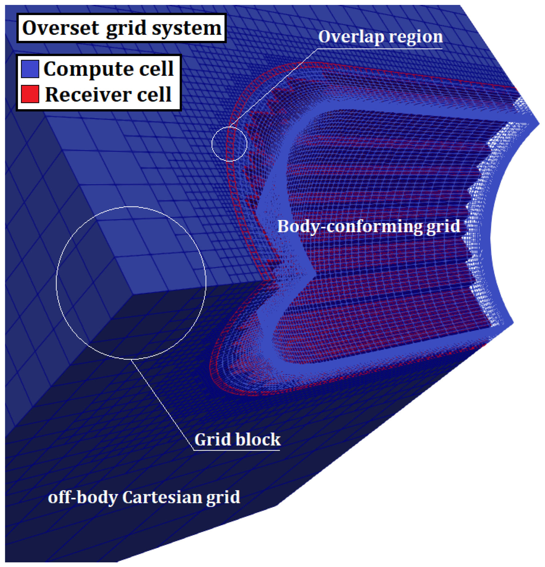
Figure 1. The overset grid system consisting of two grids, the off-body Cartesian grid and the body-conforming grid (a collection of 2 × 2 × 2 grid blocks).
Aerospace 13 00656 g001
Figure 2. The typical p4est data allocation of the nodes’ flow-field properties in the memory.
Aerospace 13 00656 g002
Figure 3. The proposed p4est decoupled interfacing with the flow-field properties.
Aerospace 13 00656 g003
Figure 4. The coarsening operation on a set of nodes marked in green for coarsening (left) and its aftermath (right). The opposite direction refers to the re-balance operation where the node violating the balance, marked in red, is reverted.
Aerospace 13 00656 g004
Figure 5. The bounding box representation of two off-body Cartesian grid partitions and a body-conforming grid partition. Each partition is assigned to a different MPI rank as labeled.
Aerospace 13 00656 g005
Figure 6. A group of cells indexed 1 to 11 in an example of a simple body-conforming grid (left) and their ADT representation (right).
Aerospace 13 00656 g006
Figure 7. The Cartesian grid governing node system (left) and its digital tree representation (right) in a two-dimensional setting is illustrated (Quadtree). The three-dimensional setting follows the same suit with an octree.
Aerospace 13 00656 g007
Figure 8. The inter-grid communication is shown. The off-body Cartesian grid donor cells’ flow-field communication process to their correspondent body-conforming grid receiver cells’ holding cores. Dashed lines are dummy transfers.
Aerospace 13 00656 g008
Figure 9. The computational domain and its assigned boundary conditions. The free stream boundary condition is applied to the transparent faces of the domain.
Aerospace 13 00656 g009
Figure 10. The coefficient of pressure distribution along the geometry’s surface. The grid convergence test (left). The present study results are compared with reference experimental [44] and numerical data [45] (right).
Aerospace 13 00656 g010
Figure 11. Numerical schlieren image superimposed with adapted grid lines (left) and the corresponding Mach contour plot (right).
Aerospace 13 00656 g011
Figure 12. The recorded speed-up factor (left) and parallel efficiency (right) with respect to different MPI rank count for both the flow solver and its interpolation subroutine.
Aerospace 13 00656 g012
Figure 13. The partitioning of a 4-node system by the z-curve and a classic slicing partitioning algorithm.
Aerospace 13 00656 g013
Figure 14. The computational domain of the shock diffraction problem. The boundary conditions are marked (left) and the regions of different flow conditions, split by the planar shock wave, are indicated (right).
Aerospace 13 00656 g014
Figure 15. Comparison of the present study’s numerically obtained schlieren image with that obtained from the conducted experiment by [46]. Reprinted with permission from Cambridge University Press.
Aerospace 13 00656 g015
Figure 16. The flow-field numerical schlieren (upper) and Mach contour (lower) evolution as well as grid adaptation at different non-dimensional times.
Aerospace 13 00656 g016
Figure 17. The wall-clock time of the AMR and flow solver single iteration (left) and the AMR’s segments (right) with respect to different MPI rank counts.
Aerospace 13 00656 g017
Figure 18. The speed-up factors (left) and parallel efficiencies (right) of the present solver and the AMR with respect to different MPI rank counts.
Aerospace 13 00656 g018
Figure 19. The CPU normalized workload of each MPI rank at MPI rank count of 32 with and without load balancing after AMR.
Aerospace 13 00656 g019
Table 1. The flow-field freestream properties.
PropertyValue
Mach2
Reynolds353,100
Temperature (T, K)242.3
Turbulence intensity0.05%
Table 2. The flow internal field initial conditions at different regions.
PropertyRegion 1Region 2
Density ( ρ , kg/ m 3 )5.14320141.4
Temperature (T, K)0.0061236760.002487067
Velocity (V, m/s)2.04511680
Disclaimer/Publisher’s Note: The statements, opinions and data contained in all publications are solely those of the individual author(s) and contributor(s) and not of MDPI and/or the editor(s). MDPI and/or the editor(s) disclaim responsibility for any injury to people or property resulting from any ideas, methods, instructions or products referred to in the content.