Physics-Constrained Relative-State Prediction of Encounter Point and Encounter Time for Penetration Decision Support

Abstract

In the information-supported penetration scenario, the predicted encounter point and encounter time can provide the future spatial threat position and the time margin for avoidance maneuver, respectively, which are important prior information for dangerous-area judgment, avoidance triggering, and penetration decision making. However, the data-driven prediction method based on absolute coordinates is likely to depend on the fixed training airspace, resulting in insufficient cross-space generalization ability. Meanwhile, the unconstrained prediction space will lead to an excessively large sample size and an unbalanced sample distribution. Aiming at the above problems, this paper proposes a physics-constrained relative-state prediction framework for the rapid prediction of the encounter point and encounter time. Firstly, the relative-state input centered on the maneuvering vehicle is adopted to reduce the dependence of the model on the fixed global coordinate system. Secondly, a concentric double-layer spherical-shell detectable threat domain is constructed to limit the approximately unbounded prediction space to a finite region that satisfies the sensor detection condition and the maneuvering constraint of the maneuvering vehicle. Furthermore, a physical geometric stratified sampling strategy based on relative distance, azimuth angle, and pitch angle is designed, and a sample-weight correction mechanism is combined to improve the balance of sample coverage under different distance layers and incoming directions. Finally, a ResNet-MLP joint regression model is constructed and trained using offline numerical simulation samples, which is used as an online rapid predictor. The simulation results show that, on the stratified training subset, the mean absolute error of the proposed model for encounter time is 0.1775 s, and the three-dimensional Euclidean error of the encounter point is 129.89 m. The tests with spatial position variation and bounded measurement noise further verify the generalization ability and robustness of the model. The proposed method can provide rapid spatial threat information and time-margin information for dynamic penetration decision making and reduce the computational requirement of repeated online numerical propagation.

1. Introduction

With the development of modern air defense and flight vehicle systems toward long-range detection, networked cooperation, and high-precision hit-to-kill encounter, the encounter threat faced by the maneuvering vehicle during flight is significantly enhanced [1,2,3,4,5]. The maneuvering vehicle can no longer meet the requirements of high-intensity penetration only by passive avoidance based on instantaneous situation information. It is urgent to predict the encounter situation in advance based on external detection information, so as to provide reliable prior support for maneuver avoidance decision making and improve the penetration survivability and mission success rate [6].

In the penetration decision-making process, the predicted encounter point and encounter time are two key quantities for describing the future encounter threat. Among them, the predicted encounter point reflects the spatial position where the maneuvering vehicle may encounter in the future, which can be used to construct the dangerous area, judge the threat direction, and assist in determining the avoidance maneuver direction. The predicted encounter time reflects the remaining time margin that the maneuvering vehicle can use for avoidance maneuver, which can provide a basis for maneuver triggering time, overload allocation, and online replanning. If these two quantities cannot be obtained rapidly, the penetration decision can only rely on the current observation state, which is likely to cause response delay. Therefore, the rapid prediction of the encounter point and encounter time is not a simple trajectory extrapolation problem but a key front-end information-support link in the penetration decision-making system.

Around the prediction problems of the encounter point, encounter time, and related encounter states, existing studies mainly include analytical or semi-analytical prediction methods, numerical propagation methods, and data-driven prediction methods. Early studies mostly established prediction methods based on kinematic relationships and encounter geometric models. Zhang et al. [7] calculated the predicted impact point or predicted encounter point through an iterative flight-time method and estimated the remaining flight time by using the relationship between the projectile–target distance and the closing velocity. Zhao et al. [8] approximated the trajectory of the approaching vehicle flying to the predicted encounter point as a linear form based on the simplified encounter geometric relationship so as to realize encounter point prediction. Hahn et al. [9] linearized the equations of motion in the high-altitude encounter process, derived the analytical expression of the approaching vehicle trajectory, and further solved the encounter time and miss distance. Dwivedi et al. [10] studied the generalized state estimation and model predictive guidance problems and improved the guidance and prediction performance by predicting the zero-effort miss distance and the remaining flight time. These methods have the advantages of clear physical meaning, high computational efficiency, and easy engineering implementation and can effectively complete encounter-state estimation under specific engagement assumptions and guidance conditions.

It should be noted that, within the finite detectable threat range, single numerical propagation is usually feasible and accurate. Therefore, this paper does not consider that numerical propagation cannot complete encounter situation prediction within a finite distance. The problem considered in this paper lies in the online repeated calling requirement in the dynamic penetration decision-making process. When the approaching vehicle enters the detectable threat domain, the maneuvering vehicle needs to perform multiple repeated predictions with the update of the observation state and may also need to evaluate the future threat states under different candidate avoidance maneuver schemes at the same time. At this time, if each prediction or each candidate scheme depends on complete numerical analysis, the computational burden will rapidly accumulate with the number of repeated predictions and candidate actions, thus affecting the efficiency of online decision making. Therefore, while maintaining acceptable prediction accuracy, using offline numerical simulation to train an online surrogate prediction model that can be rapidly called is a feasible idea to improve the efficiency of penetration decision making. Similar ideas have also been reported in aerospace trajectory prediction. For example, Yang et al. [11] developed a DNN-based real-time trajectory prediction method for rocket-powered vehicles and showed that the learned trajectory generator can significantly reduce the online computation time compared with traditional iterative trajectory calculation.

In recent years, machine learning and deep learning methods have provided new solutions for ballistic prediction, target recognition, intelligent guidance, and attack–defense confrontation decision making. Shen et al. [12] studied the penetration trajectory optimization problem of hypersonic vehicles under the threat of two approaching vehicles, which provides a reference for trajectory planning in complex threat environments. Jiang et al. [13] proposed an anti-encounter guidance method for hypersonic glide vehicles based on deep reinforcement learning, which was used to solve the decision-making problem between target strike and approaching vehicle avoidance. Sun et al. [14] proposed an improved LSTM trajectory prediction method to improve the prediction accuracy of the future trajectory of maneuvering targets. Wang et al. [15] further studied a three-dimensional integrated guidance and control method based on deep reinforcement learning, so as to enhance the adaptability in high-maneuvering encounter scenarios. Zang et al. [16] combined data-driven and knowledge-driven methods to improve the trajectory prediction accuracy of ballistic flight vehicles in the boost phase. Han et al. [17] carried out ballistic target recognition based on multi-source data representation and deep learning methods. These studies show that learning-based methods can extract the mapping relationship between the current state and future results in complex nonlinear tasks and provide a useful supplement to traditional analytical modeling and numerical propagation methods.

For the prediction of the encounter point and encounter time, some scholars have also tried to introduce neural networks and machine learning methods. Lee et al. [18] proposed a rapid calculation method for the predicted encounter point of ballistic flight vehicle defense based on neural network learning. By using the neural network to approximate the nonlinear motion law of the reentry ballistic target, the future target position can be rapidly estimated. Gao et al. [19] proposed an improved support vector regression method for the prediction of the encounter point and encounter time and improved the prediction performance by optimizing feature extraction and model parameter selection. This type of data-driven method can use offline simulation samples to learn the nonlinear mapping from the initial engagement state to the future encounter result. After training, the prediction result can be rapidly output through one forward calculation, thereby avoiding online repeated numerical propagation. However, existing data-driven prediction methods still face three key problems.

Firstly, when the absolute coordinates of the projectile bodies in the inertial coordinate system are used as the input of the prediction model, the model is likely to fit the global spatial distribution of the training samples rather than the physically meaningful relative engagement law between the maneuvering vehicle and the approaching vehicle. When the whole engagement airspace is translated or the target state exceeds the main coverage region of the training samples, the absolute-coordinate input may cause obvious distribution shift, thereby reducing the spatial generalization ability of the model and limiting its continuous online prediction application in different missions. Therefore, this paper selects a relative-state representation scheme centered on the maneuvering vehicle and uses the position and direction of the approaching vehicle relative to the maneuvering vehicle and the motion state of the maneuvering vehicle itself to construct the model input. In this way, the model focuses on learning the relative motion law, removes the dependence on fixed spatial coordinates, improves the spatial translation generalization performance of the model, and adapts to the engineering requirements of prediction in penetration scenarios.

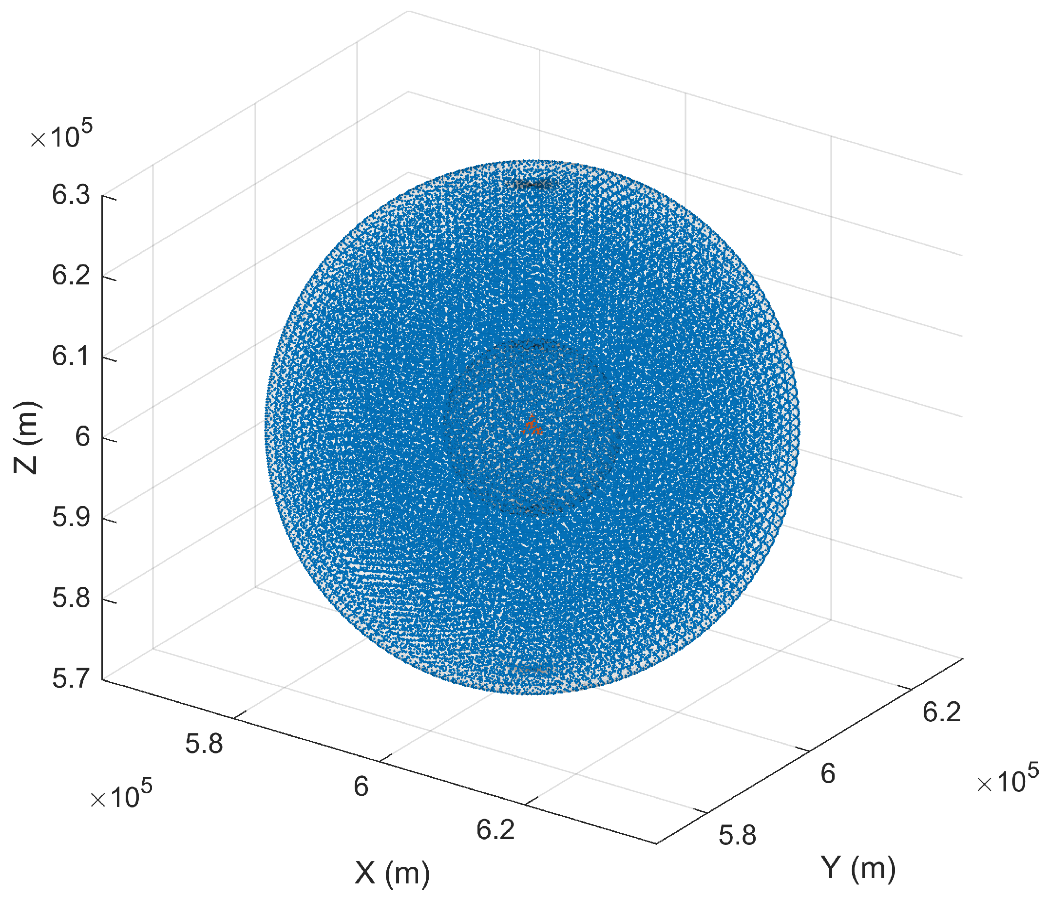
Secondly, unconstrained full-domain prediction will make the input space of the approaching vehicle nearly unbounded. This will not only make the training sample size difficult to control but also reduce the engineering significance of long-distance prediction results for the current penetration decision. Based on this, this paper constructs a concentric double-layer spherical-shell detectable threat domain centered on the maneuvering vehicle. The outer boundary is used to limit the effective detection distance of the sensor and is helpful to improve the prediction accuracy of the model so that the originally unbounded spatial prediction problem is transformed into a bounded prediction problem with clear physical meaning. Meanwhile, the model input interval is narrowed to control the sample size. The inner boundary based on the maneuvering performance of the projectile is defined as the safety critical distance at which the maneuvering vehicle retains the avoidance margin. In this way, the detection condition, projectile maneuvering limitation, and model generalization boundary are integrated by means of the double-layer spherical shell, and the unbounded spatial prediction is transformed into finite-domain prediction with clear physical meaning.

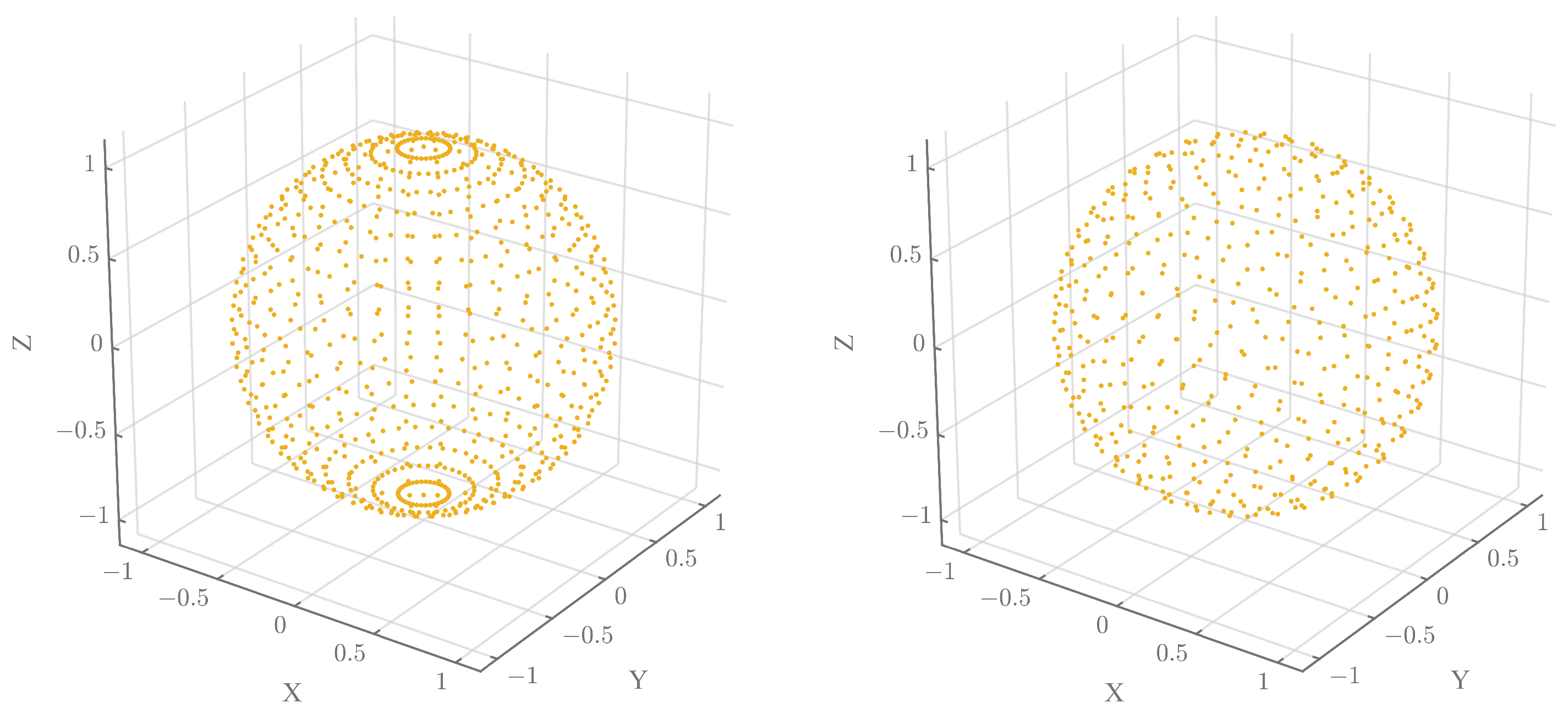
Furthermore, even if the finite threat domain of the double-layer spherical shell is defined, the surface area of the three-dimensional spherical shell increases with the radius, and different angular engagement configurations are different. Irregular random sampling is likely to cause an unbalanced spatial sample distribution, resulting in insufficient samples in some distance and direction regions and high local prediction errors. Aiming at this problem, this paper carries out physical geometric stratification of the engagement space based on relative distance, azimuth angle, and pitch angle and combines stratified sampling with sample-weight correction to balance the sample coverage of the whole airspace under the premise of reducing the total sample size.

Accordingly, this paper establishes a physics-constrained relative-state rapid prediction framework for penetration decision making. Firstly, the effective prediction airspace [20] with practical decision-making value is defined based on the maneuvering vehicle-centered double-layer spherical shell. Then, stratified sampling [21,22] is carried out in the domain based on the dimensions of distance, azimuth, and pitch, and weight correction [23] is supplemented to balance the sample distribution in the whole space. Subsequently, a ResNet-MLP joint regression model is established to complete the end-to-end rapid fitting from the relative engagement state to the encounter parameters.

For the penetration decision-making task considered in this study, the predicted encounter point and encounter time are intended to provide front-end information for subsequent maneuver decision and trajectory replanning. The trustworthiness and physical interpretability of the predictor should also be considered, such as in the decision-tree-based pilot workload prediction [24]. Inspired by this concern, the present study improves the engineering interpretability of the rapid predictor mainly through physically meaningful relative-state inputs, a bounded detectable-region formulation, and statistical error evaluation of the predicted encounter point and encounter time.

The main contributions are summarized as follows:

• A relative-state encounter prediction modeling method is proposed for penetration decision making. The model improves the spatial generalization ability.
• A concentric double-layer spherical-shell detectable threat domain is constructed. The prediction space avoids the uncontrollable sample-size problem caused by unbounded spatial prediction.
• A physical geometric stratified sampling strategy is designed and combined with a sample-weight correction mechanism to reduce the training data scale while maintaining prediction accuracy comparable to that of the full training dataset.

The remainder of this paper is organized as follows. Section 2 presents the problem formulation. Section 3 introduces the engagement kinematic model. Section 4 describes the dataset construction method. Section 5 presents the surrogate regression predictor. Section 6 discusses the prediction results. Section 7 presents the generalization analysis. Section 8 presents the robustness analysis. Finally, Section 9 concludes this paper.

2. Problem Description

A three-entity engagement process in a modern penetration scenario is considered [25]. During the strike mission, the approaching vehicle attempts to intercept the maneuvering vehicle, whereas the information-support platform performs aerial surveillance and provides external information support to the maneuvering vehicle through a data link. The information-support platform may include an early-warning aircraft, fighter aircraft, cooperative unmanned aerial vehicle, ground-based radar, reconnaissance satellite, or other assets with air-surveillance capability. Owing to its wide detection coverage, the platform can search for and track the approaching vehicle at an early stage while maintaining a safe stand-off distance [26]. Once the approaching vehicle enters the concentric spherical-shell region, the platform obtains effective observations and transmits the measurement data to the maneuvering vehicle through the data link.

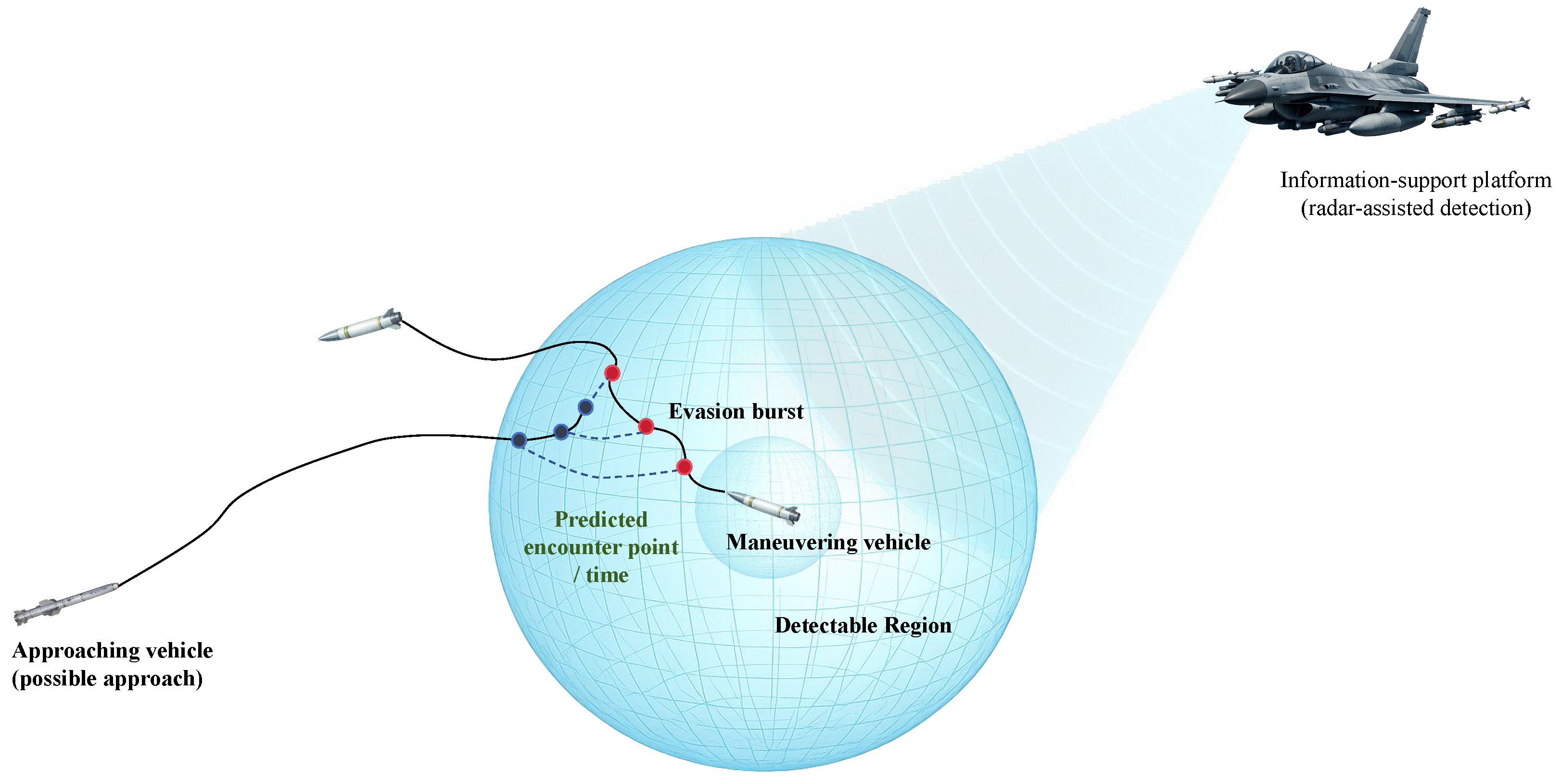
To describe the effective spatial extent of the detectable region under information-support conditions, as shown in Figure 1, the detectable region is equivalently modeled as concentric spherical shells centered on the maneuvering vehicle. Let the inner-boundary radius be $R_{\min }$, which is related to the minimum theoretical turning radius and maneuvering capability of the maneuvering vehicle. If the approaching vehicle has already entered the inner boundary, the system may still provide predictions of the encounter point and encounter time. However, the available reaction time and evasive distance become very limited, and the feasibility of successful avoidance based only on the maneuvering vehicle’s maximum maneuvering capability is significantly reduced.

Figure 1. Detectable-region diagram.

The outer-boundary radius $R_{\max }$ is determined by considering sensor detection capability, sample coverage, and prediction reliability. If the outer boundary is extended excessively, the prediction model needs more samples to represent the nonlinear engagement relationships over a larger spatial region. This increases the data scale and may also enlarge local extreme prediction errors, thereby reducing the practical relevance of long-distance prediction results for immediate maneuver decision making. Therefore, the system considers the current observation conditions suitable for prediction and evasive decision support only when the approaching vehicle is located within the region bounded by $R_{\min }$ and $R_{\max }$.

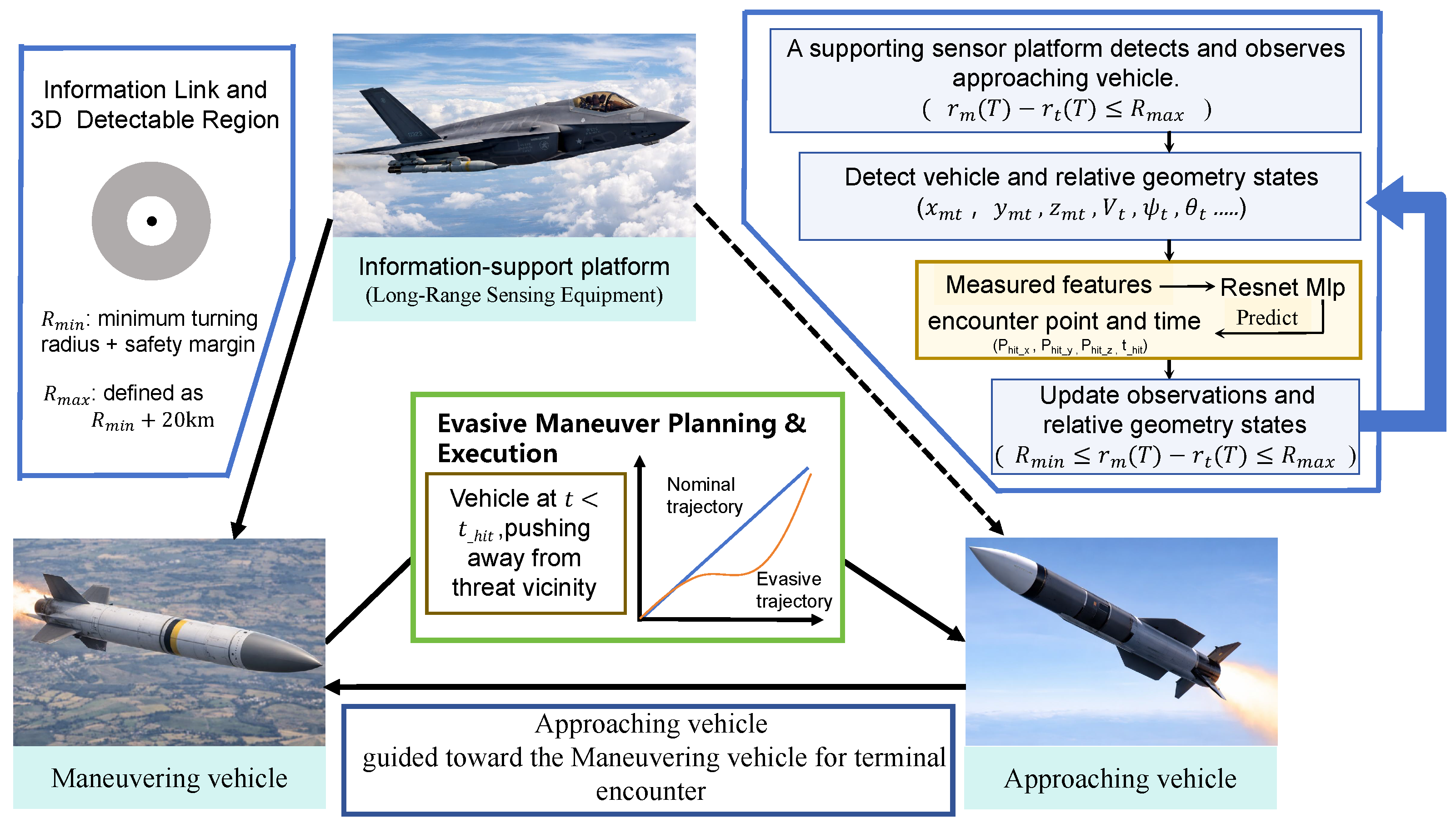
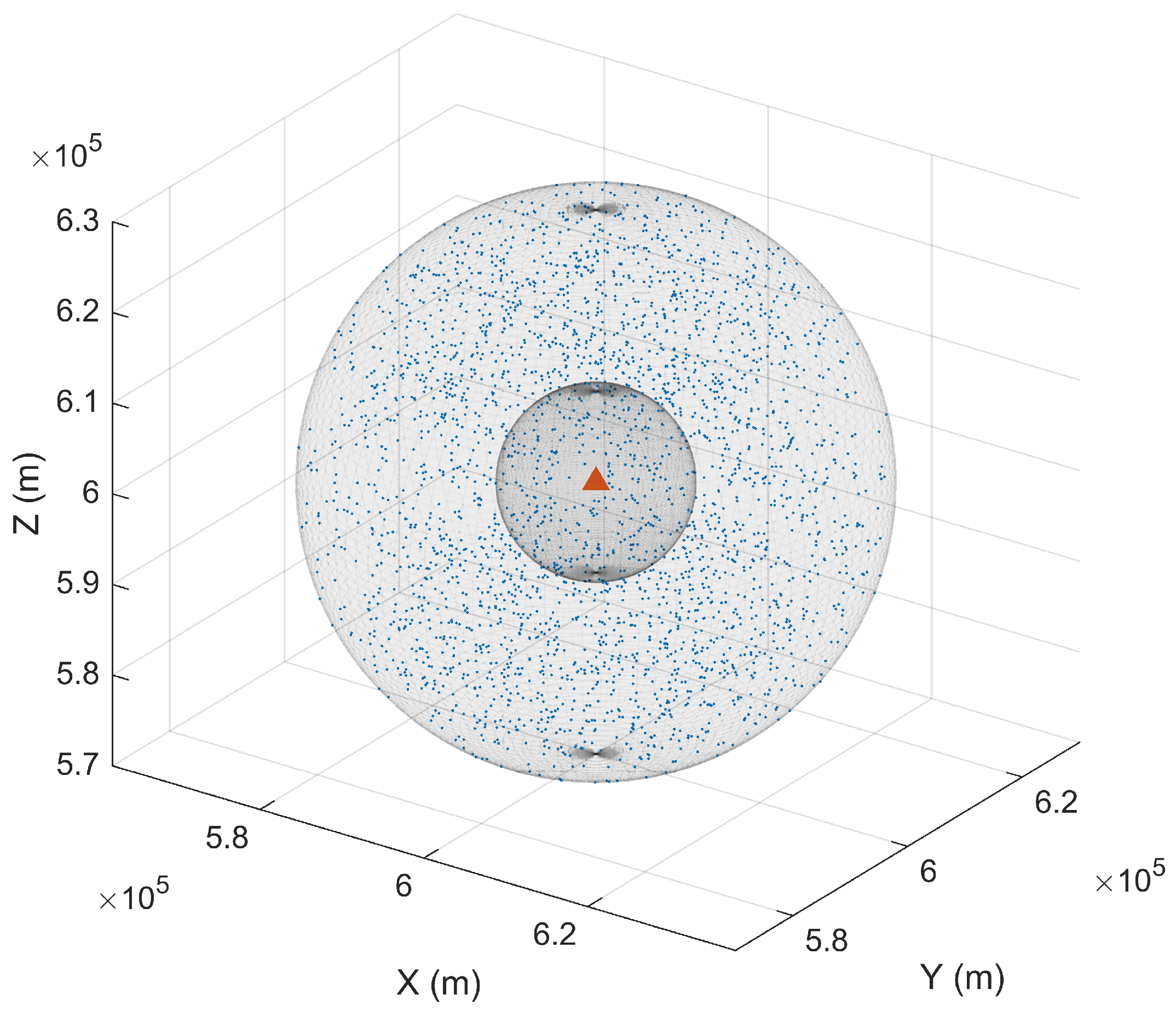
When the approaching vehicle first enters the detectable region, this moment is defined as the first detection point. From this moment on, the system uses the currently available relative-state information to rapidly predict the encounter point and encounter time in the future engagement process. The prediction results provide front-end information for subsequent evasive decision making. During the subsequent flight process, this prediction process can be repeated as the observations are updated, as shown in Figure 2. It should be noted that this study focuses on the rapid prediction module, while the complete closed-loop evasive decision law is left for future work.

Figure 2. Schematic diagram of the engagement process.

3. Engagement Kinematic Model

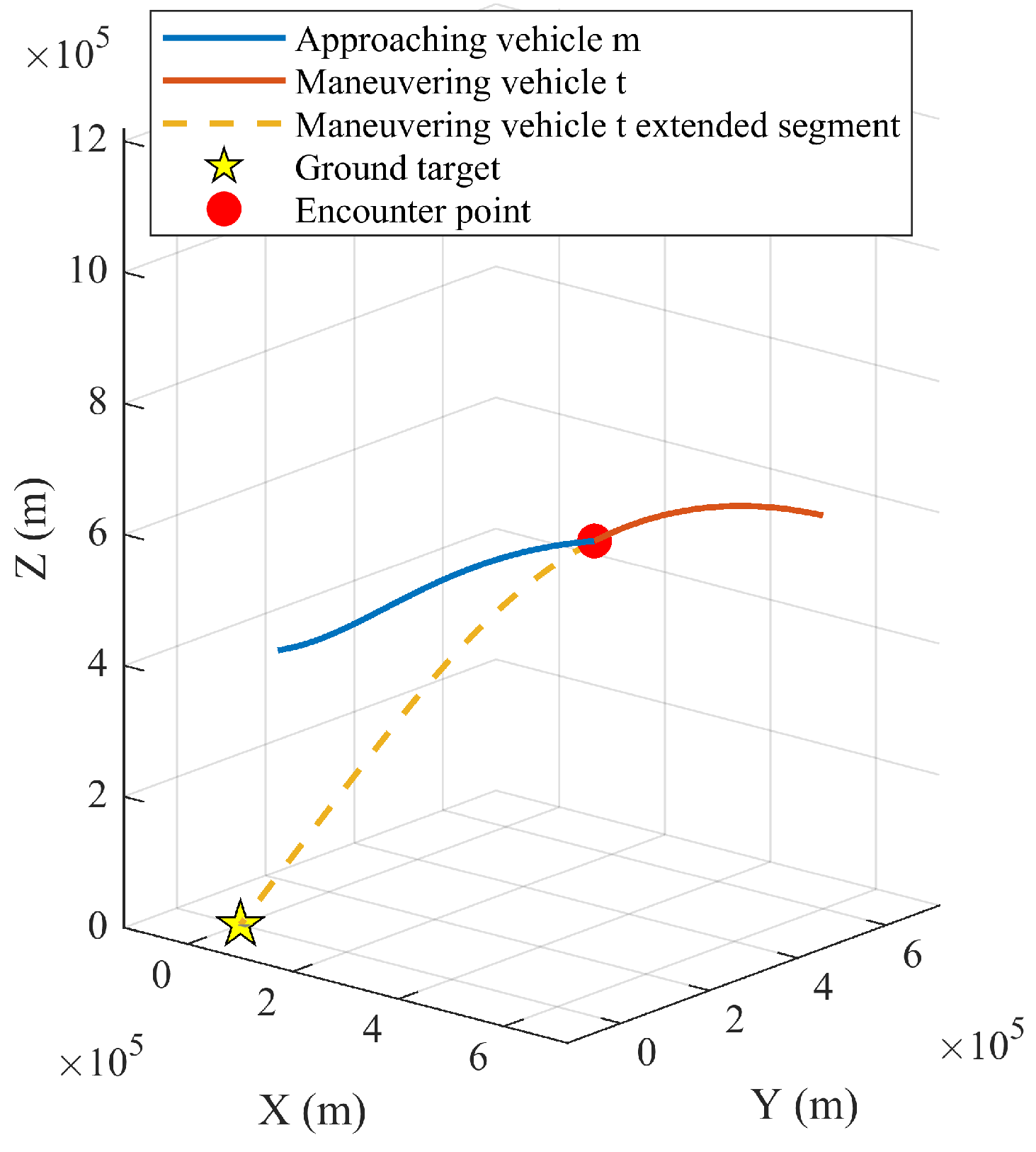
A simulation scenario in three-dimensional space is considered [27], as shown in Figure 3. The approaching vehicle m uses proportional navigation to encounter the maneuvering vehicle t, while the maneuvering vehicle t simultaneously uses proportional navigation to strike the ground target g. The simulation needs to output the precise coordinates of the encounter point and the encounter time when the maneuvering vehicle is hit by the approaching vehicle.

Figure 3. Engagement simulation diagram.

Since the flight time within the detectable region is relatively short, the maneuvering flight process of the approaching vehicle and the maneuvering vehicle in three-dimensional space is described by assuming that both the approaching vehicle and the maneuvering vehicle move at constant speed and that acceleration only changes the direction of velocity. Their three-dimensional position vectors are defined as follows:

$${\mathbf{r}}_m={\left[x_m{y}_m{z}_m\right]}^{\mathrm{T}},{\mathbf{r}}_t={\left[x_t{y}_t{z}_t\right]}^{\mathrm{T}},{\mathbf{r}}_g={\left[x_g{y}_g{z}_g\right]}^{\mathrm{T}}$$

Then, the relative position and distance are given by

$$\begin{array}{ccc}\hfill {\mathbf{r}}_{mt}& ={\mathbf{r}}_t-{\mathbf{r}}_m,\hfill & \hfill R_{mt}= \parallel {\mathbf{r}}_{mt}\parallel ,\\ \hfill {\mathbf{r}}_{tg}& ={\mathbf{r}}_g-{\mathbf{r}}_t,\hfill & \hfill R_{tg}= \parallel {\mathbf{r}}_{tg}\parallel .\end{array}$$

(1)

$V_m$ and $V_t$ denote the constant speeds of the approaching vehicle and the maneuvering vehicle, respectively, with their velocity directions represented by the unit vectors ${\widehat{\mathbf{v}}}_m$ and ${\widehat{\mathbf{v}}}_t$. Therefore, the velocity vectors are ${\mathbf{v}}_m=V_m{\widehat{\mathbf{v}}}_m$ and ${\mathbf{v}}_t=V_t{\widehat{\mathbf{v}}}_t$. At the same time, $\psi$ is yaw angle and $\theta$ is pitch angle, thus $a_{\theta ,m}$ and $a_{\psi ,m}$ denote the normal acceleration components in the pitch and yaw planes, respectively.

The kinematic and dynamic equations of the approaching vehicle m relative to the maneuvering vehicle t:

$$\left\{\begin{array}{cc}\hfill {\dot{x}}_m& =V_m\cos {\theta }_m\cos {\psi }_m\hfill \\ \hfill {\dot{y}}_m& =V_m\cos {\theta }_m\sin {\psi }_m\hfill \\ \hfill {\dot{z}}_m& =V_m\sin {\theta }_m\hfill \\ \hfill {\dot{V}}_m& =0\hfill \\ \hfill {\dot{\theta }}_m& ={\displaystyle \frac{a_{\theta ,m}}{V_m}}\hfill \\ \hfill {\dot{\psi }}_m& ={\displaystyle \frac{a_{\psi ,m}}{V_m\cos {\theta }_m}}\hfill \end{array}\right.$$

(2)

The kinematic and dynamic equations of the maneuvering vehicle t relative to the ground target g have the same form as above, therefore details are omitted.

Line-of-Sight Rate and Proportional Navigation

The relative velocity vector is defined as ${\mathbf{v}}_{\mathrm{rel}}={\mathbf{v}}_m-{\mathbf{v}}_t$. The three-dimensional line-of-sight angular velocity vector is

$${\mathit{\omega }}_{\mathrm{los}}={\displaystyle \frac{{\mathbf{r}}_{mt}\times {\mathbf{v}}_{rel}}{\parallel {\mathbf{r}}_{mt}{\parallel }^2}}.$$

(3)

The unit line-of-sight vector is defined as $\widehat{\mathbf{r}}={\displaystyle \frac{{\mathbf{r}}_{mt}}{\parallel {\mathbf{r}}_{mt}\parallel }}$, and the closing speed is

$$V_c=\max \left(0,-{\displaystyle \frac{{\mathbf{r}}_{mt}^{\mathrm{T}}{\mathbf{v}}_{rel}}{\parallel {\mathbf{r}}_{mt}\parallel }}\right).$$

(4)

Proportional navigation’s basic principle is to generate the normal acceleration of the vehicle in proportion to the line-of-sight angular rate. Its form is ${\mathbf{a}}_{\mathrm{cmd}}=N{V}_c\left({\mathit{\omega }}_{\mathrm{los}}\times \widehat{\mathbf{r}}\right)$, where N is the proportional navigation gain ($N_t=5$, $N_m=6$). To preserve constant speed and avoid tangential acceleration, ${\mathbf{a}}_{cmd}$ is projected onto the plane orthogonal to the approaching vehicle velocity direction, and only its normal component is retained, thus giving

$${\mathbf{a}}_m=\left(\mathbf{I}-{\widehat{\mathbf{v}}}_m{\widehat{\mathbf{v}}}_m^{\mathrm{T}}\right){\mathbf{a}}_{\mathrm{cmd}}.$$

(5)

For the guidance of the maneuvering vehicle t toward the ground target g, it is only necessary to replace the relative quantity with ${\mathbf{r}}_{tg}={\mathbf{r}}_g-{\mathbf{r}}_t$ and ${\mathbf{v}}_{\mathrm{rel},tg}=-{\mathbf{v}}_t$; accordingly, the closing speed can be written as

$$V_c^{tg}=\max \left(0,{\displaystyle \frac{{\mathbf{r}}_{tg}^{\mathrm{T}}{\mathbf{v}}_t}{\parallel {\mathbf{r}}_{tg}\parallel }}\right).$$

(6)

4. Dataset Construction

Since real engagement data are difficult to obtain and are limited in public release, annotation, and condition coverage, this study uses a physics-constrained numerical simulation method to generate the training and test datasets. The simulation-based dataset construction can cover different initial relative positions, incoming directions, and distance-layer conditions in a controllable way, thereby providing data support for model training and validation.

4.1. Training Dataset Construction

4.1.1. Detectable Threat Region and Full Position Sampling

In this study, the detectable threat region is used as the sample space for constructing the initial approaching vehicle positions. It is modeled as a set of concentric spherical shells centered on the maneuvering vehicle. The inner boundary radius is set to $R_{\min }=10\mathrm{km}$, and the outer boundary radius is set to $R_{\max }=30\mathrm{km}$. Accordingly, the detectable threat region can be expressed as

$$D=\left\{R_{\min }\le ∥{\mathbf{r}}_m-{\mathbf{r}}_t∥\le R_{\max }\right\},$$

(7)

where ${\mathbf{r}}_m$ and ${\mathbf{r}}_t$ denote the positions of the approaching vehicle and the maneuvering vehicle, respectively.

The detectable threat region is discretized into L concentric spherical shells with radius

$$R_k\in \left\{10\mathrm{km},11\mathrm{km},\dots ,30\mathrm{km}\right\},k=1,2,\dots ,L.$$

(8)

To keep the full dataset at a controllable scale, an initial sample budget is first estimated using a reference surface spacing. For the spherical shell with radius $R_k$, the reference spacing is defined as

$$s\left(R_k\right)=s_0{\left({\displaystyle \frac{R_{\max }}{R_k}}\right)}^{\gamma },$$

(9)

where $s_0$ is the reference spacing on the outermost shell and $\gamma$ controls the variation of the estimated spacing with radius. The corresponding estimated number of points on the k-th shell is

$${\tilde{N}}_k=⌈{\displaystyle \frac{4\pi R_k^2}{s{\left(R_k\right)}^2}}⌉.$$

(10)

To avoid too few or too many samples on a single shell, the estimated number is bounded by

$${\tilde{N}}_k=\max \left(N_{\min },\min \left({\tilde{N}}_k,N_{\max }\right)\right),$$

(11)

where $N_{\min }=12$ and $N_{\max }$ = 30,000. The total sample budget is then estimated as

$$B={\displaystyle \sum _{k=1}^L}{\tilde{N}}_k.$$

(12)

It should be noted that the spacing function is only used to estimate the total sample budget. The actual sample quota of each shell is assigned according to the shell surface area. Since the surface area of a spherical shell increases with the radius, more samples are assigned to outer shells to maintain approximately uniform geometric coverage. The area-based weight of the k-th shell is defined as

$${\omega }_k={\displaystyle \frac{R_k^2}{{\sum }_{l=1}^L{R}_l^2}}.$$

(13)

The initial sample quota of the k-th shell is then given by

$$N_k=⌊B{\omega }_k+0.5⌋.$$

(14)

After rounding, the quotas are adjusted under the constraints $N_{\min }\le N_k\le N_{\max }$ to satisfy

$${\displaystyle \sum _{k=1}^L}{N}_k=B.$$

(15)

In this way, the initial full position samples are distributed according to the surface-area difference among different spherical shells, while the total number of samples remains controllable.

4.1.2. Fibonacci Sphere Sampling

For the k-th spherical shell with radius $R_k$, $N_k$ sample points are generated on its surface to define the initial positions of the approaching vehicle. Traditional latitude–longitude grid sampling may produce dense points near the poles and sparse points near the equator because the cell area changes with latitude. This uneven distribution may introduce sampling bias. Therefore, Fibonacci sphere sampling is adopted to obtain more uniform directional coverage on each spherical shell. The comparison between latitude–longitude grid sampling and Fibonacci sphere sampling is shown in Figure 4.

Figure 4. Comparison of sphere sampling methods.

Let ${\varphi }_g=(1+\sqrt{5})/2$ be the golden ratio. For the i-th point on the k-th spherical shell, where $i=0,1,\dots ,N_k-1$, the vertical coordinate and the corresponding radial projection are given by

$$z_i=1-{\displaystyle \frac{2(i+0.5)}{N_k}},{\rho }_i=\sqrt{1-z_i^2}.$$

(16)

The azimuth angle is defined as

$${\phi }_i={\displaystyle \frac{2\pi i}{{\varphi }_g}}.$$

(17)

Thus, the unit direction vector of the i-th point is

$${\mathbf{d}}_i^{\left(k\right)}=\left[\begin{array}{c}{\rho }_i\cos {\phi }_i\\ {\rho }_i\sin {\phi }_i\\ z_i\end{array}\right].$$

(18)

The corresponding initial position of the approaching vehicle is generated as

$${\mathbf{r}}_{m,i}^{\left(k\right)}={\mathbf{r}}_t+R_k{\mathbf{d}}_i^{\left(k\right)}.$$

(19)

The relative position vector from the sampled approaching vehicle position to the maneuvering vehicle is defined as

$$\Delta {\mathbf{r}}_{mt}={\mathbf{r}}_t-{\mathbf{r}}_{m,i}^{\left(k\right)}={\left[\begin{array}{ccc}\Delta x_{mt}& \Delta y_{mt}& \Delta z_{mt}\end{array}\right]}^{\mathrm{T}}.$$

(20)

Based on this vector, the corresponding relative distance, yaw angle, and pitch angle are calculated by

$$r_{mt}=\sqrt{\Delta x_{mt}^2+\Delta y_{mt}^2+\Delta z_{mt}^2},$$

(21)

$${\psi }_{mt}=\mathrm{mod}\left(\mathrm{atan}2\right(\Delta y_{mt},\Delta x_{mt}),2\pi ),$$

(22)

$${\theta }_{mt}=\mathrm{atan}2\left(\Delta z_{mt},\sqrt{\Delta x_{mt}^2+\Delta y_{mt}^2}\right).$$

(23)

The full approaching vehicle-position dataset generated by Fibonacci sphere sampling is shown in Figure 5.

Figure 5. Full dataset distribution.

4.1.3. Stratified Training Subset and Sample Weighting

After the full approaching vehicle-position dataset is constructed, a stratified training subset is further generated to reduce the training data scale while retaining representative spatial coverage. The stratification is performed according to the relative distance $r_{mt}$, yaw angle ${\psi }_{mt}$, and pitch angle ${\theta }_{mt}$.

Specifically, the relative distance $r_{mt}$ is divided into $n_r=4$ bins according to quantiles. The yaw angle ${\psi }_{mt}$ is divided into equal-width bins with an interval of $\Delta \psi ={30}^{\circ }$. The pitch angle ${\theta }_{mt}$ is divided into three equal-width bins:

$$[-{90}^{\circ },-{30}^{\circ }],[-{30}^{\circ },{30}^{\circ }],[{30}^{\circ },{90}^{\circ }].$$

(24)

Therefore, each sample is assigned to a discrete cell

$$c=\left(r_{\mathrm{bin}},{\psi }_{\mathrm{bin}},{\theta }_{\mathrm{bin}}\right).$$

(25)

Let $N_{\mathrm{pop}}\left(c\right)$ denote the number of full-dataset samples in cell c. To construct the stratified subset, at most K samples are selected from each cell:

$$N_{\mathrm{sub}}\left(c\right)=\min \left(N_{\mathrm{pop}}\left(c\right),K\right),$$

(26)

where $K=20$ in this study. If $N_{\mathrm{pop}}\left(c\right)\le K$, all samples in this cell are retained. Otherwise, K samples are randomly selected from this cell. In this way, the stratified subset avoids being dominated by densely populated regions and provides more balanced coverage over different distance and angular regions. The stratified subset distribution is shown in Figure 6.

Figure 6. Stratified subset distribution.

The stratified subset improves the balance of spatial coverage, but it also changes the original distribution of the full dataset. Therefore, sample weights are introduced during training to compensate for the distribution difference between the stratified subset and the full dataset. For each cell c, the population-to-subset ratio is defined as

$$\mathrm{ratio}\left(c\right)={\displaystyle \frac{N_{\mathrm{pop}}\left(c\right)}{N_{\mathrm{sub}}\left(c\right)}}.$$

(27)

For the i-th selected sample belonging to cell $c_i$, the training weight is calculated as

$$w_i={\left[\mathrm{ratio}\left(c_i\right)\right]}^{\alpha }.$$

(28)

The weights are then normalized by their mean value:

$$w_i\leftarrow {\displaystyle \frac{w_i}{\frac{1}{N}{\sum }_{i=1}^N{w}_i}}.$$

(29)

To avoid excessively large weights, the normalized weights are clipped by an upper bound:

$$w_i\leftarrow \min \left(w_i,w_{\max }\right).$$

(30)

In this study, $\alpha =0.5$ and $w_{\max }=5$. The stratified subset is used to improve the spatial balance of the selected training samples, while the sample weights are used to preserve the distribution information of the full dataset during model training. Preliminary cross-combination experiments were conducted using $K\in \{20,25,30\}$ and $\alpha \in \{0,0.3,0.5,0.8,1.0\}$. Among the 15 tested combinations, $K=20$ and $\alpha =0.5$ achieved the best overall prediction performance while maintaining a compact training subset and stable sample-weight correction; therefore, these values were adopted in the subsequent experiments.

4.1.4. Feasible Initial Attitude Set of the Maneuvering Vehicle

After obtaining the initial position samples of the approaching vehicle, the feasible initial attitude set of the maneuvering vehicle is further constructed. For an arbitrary candidate attitude $({\psi }_t,{\theta }_t)$ of the maneuvering vehicle, the corresponding unit velocity direction vector is expressed as

$${\widehat{\mathbf{v}}}_t({\psi }_t,{\theta }_t)=\left[\begin{array}{c}\cos {\theta }_t\cos {\psi }_t\\ \cos {\theta }_t\sin {\psi }_t\\ \sin {\theta }_t\end{array}\right].$$

(31)

Let the unit line-of-sight vector from the maneuvering vehicle to the ground target be

$${\widehat{\mathbf{r}}}_{tg}={\displaystyle \frac{{\mathbf{r}}_{tg}}{∥{\mathbf{r}}_{tg}∥}}.$$

(32)

The lead angle $\delta$ between the velocity direction and the line-of-sight direction is calculated as

$$\delta =\arccos \left({\widehat{\mathbf{v}}}_t{({\psi }_t,{\theta }_t)}^{\mathrm{T}}{\widehat{\mathbf{r}}}_{tg}\right).$$

(33)

Under proportional navigation, the initial commanded normal acceleration is denoted as $a_{\mathrm{cmd}}$. To ensure that the initial guidance command is feasible, the condition $a_{\mathrm{cmd}}\le a_{\max }$ should be satisfied. The initial commanded acceleration is calculated as

$$a_{\mathrm{cmd}}={\displaystyle \frac{N_t{V}_t^2\sin 2\delta }{2R_{tg}}}.$$

(34)

Accordingly, the maximum allowable lead angle is obtained as

$${\delta }_{\max }=\left\{\begin{array}{cc}{\displaystyle \frac{1}{2}}\arcsin \left({\displaystyle \frac{2a_{\max }{R}_{tg}}{N_t{V}_t^2}}\right),\hfill & {\displaystyle \frac{2a_{\max }{R}_{tg}}{N_t{V}_t^2}}<1,\hfill \\ {90}^{\circ },\hfill & {\displaystyle \frac{2a_{\max }{R}_{tg}}{N_t{V}_t^2}}\ge 1.\hfill \end{array}\right.$$

(35)

Only the yaw–pitch combinations satisfying

$$\delta \le {\delta }_{\max }$$

(36)

are retained to form the feasible initial attitude set of the maneuvering vehicle.

4.1.5. Generation of Engagement Simulation Samples

After the approaching vehicle initial positions and the feasible initial attitudes of the maneuvering vehicle are determined, three-dimensional engagement simulations are carried out to generate the prediction labels. The initial position of the approaching vehicle is determined by the sampled points within the detectable threat region, and its initial attitude is initialized to point toward the initial position of the maneuvering vehicle. The initial position of the maneuvering vehicle is fixed at (600,000, 600,000, 600,000), and the ground target position is fixed at $(0,0,0)$. Other key parameter settings are listed in Table 1.

Table 1. Settings of key parameters.

Parameter	Sampling Range	Sampling Interval
$N_t$	5	Fixed
$N_m$	6	Fixed
$A_{m,\max }$	200	Fixed
$A_{t,\max }$	100	Fixed
$V_m$	600	Fixed
$V_t$	$[420,460]$	20
${\psi }_t$	$[0,360)$	25
${\theta }_t$	$[-70,70]$	20

The selected initial attitudes of the maneuvering vehicle are combined with the selected initial state parameters of the approaching vehicle to generate simulation samples. Specifically, each group of

$$\left(V_m,V_t,{\psi }_m,{\psi }_t,{\theta }_t,{\theta }_m,\Delta x_{mt},\Delta y_{mt},\Delta z_{mt}\right)$$

(37)

is used as the initial condition for one three-dimensional engagement simulation. The corresponding encounter point coordinates

$$\left(p_{\mathrm{hit},x},p_{\mathrm{hit},y},p_{\mathrm{hit},z}\right)$$

(38)

and encounter time $t_{\mathrm{hit}}$ are recorded as prediction labels.

Finally, a total of 19,360,824 full samples are generated by the full-combination method, and a stratified training subset with 483,840 samples is constructed for subsequent model training and performance comparison.

4.2. Independent Test Dataset Construction

To evaluate spatial generalization and avoid direct overlap between training and test samples, an independent test dataset is constructed using a different shell-point selection scheme. Within the same radial range, the test dataset does not use Fibonacci sphere sampling. Instead, the sample points on each spherical surface are generated randomly. In addition, different yaw and pitch step sizes are used, and the number of sample points and directional sequences on each shell are independently designed.

Duplicate or overlapping approaching vehicle initial-position samples between the training and test datasets are excluded. Under this setting, the test error better reflects the spatial generalization capability of the predictor to unseen approaching vehicle initial positions rather than the memorization of specific geometric configurations in the training set.

4.3. Data Preprocessing

Before training, the dataset should be normalized. Normalization can unify data of different dimensions and ranges into a standard scale; this helps remove scale differences among the data and prevents certain features from dominating the learning process of the model. It also helps accelerate convergence and improve training efficiency. The formula is as follows:

$$q_n={\displaystyle \frac{q-{\mu }_q}{{\sigma }_q}},$$

(39)

${\mu }_q$ and ${\sigma }_q$ represent the mean and standard deviation of this variable on the training set, respectively. The same normalization form is applied to both input features and output features.

5. Surrogate Regression Predictor

In this study, ResNet-MLP is used as a lightweight surrogate regression predictor within the proposed physics-constrained relative-state prediction framework. The purpose of using this model is not to introduce a fundamentally new neural-network architecture but to provide a stable and efficient nonlinear mapping from the relative engagement state to the encounter-point displacement and encounter time. The main methodological emphasis of this paper lies in the maneuvering vehicle-centered relative-state representation, bounded detectable-region modeling, geometry-stratified sampling, and generalization-oriented validation.

The model takes a nine-dimensional relative-state feature vector as input. The definitions of the input features are provided in Table 2. The network consists of an input feature normalization layer, a shared residual backbone, and four parallel MLP regression heads. The shared backbone contains five residual blocks with shortcut connections, which are introduced to improve training stability and alleviate the degradation problem in deeper feedforward networks [28]. Layer normalization, GELU activation, and dropout are used in the residual blocks and regression heads for training stabilization, nonlinear activation, and regularization, respectively [29,30,31]. The MLP regression heads are used to predict different continuous outputs because feedforward neural networks are typical nonlinear function approximators for regression tasks [32]. The hyperparameter settings of the model are summarized in Table 3.

Table 2. Definitions of input features.

Abbreviation	Description
$\Delta x_{tm}$	Relative displacement between the approaching vehicle and the maneuvering vehicle in the x direction
$\Delta y_{tm}$	Relative displacement between the approaching vehicle and the maneuvering vehicle in the y direction
$\Delta z_{tm}$	Relative displacement between the approaching vehicle and the maneuvering vehicle in the z direction
${\theta }_t$	Pitch angle of the maneuvering vehicle
${\psi }_t$	Yaw angle of the maneuvering vehicle
$v_{x,t}$	Velocity component of the maneuvering vehicle in the x direction
$v_{y,t}$	Velocity component of the maneuvering vehicle in the y direction
$v_{z,t}$	Velocity component of the maneuvering vehicle in the z direction
$V_t$	Speed of the vehicle

Table 3. Hyperparameter settings of the ResNet-MLP model.

Parameter	Setting
Dropout	0.0202016
Learning rate	$1.232191\times {10}^{-4}$
Batch size	1024
Number of epochs	100
Backbone hidden sizes	256-128-64-32-16
Number of residual blocks	5
Number of regression heads	4

After feature extraction by the shared residual backbone, the final output vector is expressed as

$$\widehat{\mathbf{y}}={\left[\begin{array}{cccc}{\widehat{\Delta x}}_{hit}& {\widehat{\Delta y}}_{hit}& {\widehat{\Delta z}}_{hit}& {\widehat{t}}_{hit}\end{array}\right]}^{\top }.$$

(40)

Here, ${\widehat{\Delta x}}_{hit}$, ${\widehat{\Delta y}}_{hit}$, and ${\widehat{\Delta z}}_{hit}$ denote the predicted displacement components of the encounter point relative to the maneuvering vehicle, and ${\widehat{t}}_{hit}$ denotes the predicted encounter time. The absolute position of the encounter point can be obtained by adding the predicted displacement vector to the current position of the maneuvering vehicle.

The model is trained in a supervised manner using the generated engagement samples. To compensate for the sample-distribution change caused by the construction of the stratified training subset, a weighted mean squared error loss is used:

$$\mathcal{L}={\displaystyle \frac{1}{N}}{\displaystyle \sum _{i=1}^N}{w}_i\left({\displaystyle \frac{1}{4}}{\displaystyle \sum _{j=1}^4}{\left({\widehat{y}}_{i,j}-y_{i,j}\right)}^2\right),$$

(41)

where ${\widehat{y}}_{i,j}$ and $y_{i,j}$ denote the predicted and true values of the j-th output of the i-th sample, respectively. For the full training dataset, $w_i=1$. For the stratified training subset, $w_i$ is assigned according to the stratified sampling procedure to reduce the distribution bias introduced by subset construction.

6. Results and Discussion

Since the training dataset used in this study is large, the benchmark models should not only provide competitive prediction accuracy but also be applicable to large-scale training and repeated online inference. Meanwhile, the problem considered in this study is a supervised regression task that maps a nine-dimensional continuous physical-state vector to four continuous encounter parameters. The input variables have explicit physical meanings, are relatively low-dimensional, and do not exhibit an inherent temporal-sequence or spatial-grid structure. Therefore, the selection of benchmark models considers model type, suitability for the present structured continuous regression task, structural complexity, training cost, and inference efficiency. Although more complex models may have stronger representation capability, they may also increase the difficulty of hyperparameter tuning and the computational burden in large-scale prediction tasks.

Based on this consideration, representative data-driven regression models with different structural characteristics are selected for comparison. XGBoost is used as a tree-based ensemble regression model, MLP as a basic feedforward neural network, ResNet as a residual neural network, and FT-Transformer as a Transformer-based model for structured tabular features. These models cover several typical surrogate regression structures and provide a comparative basis for evaluating the proposed ResNet-MLP predictor in the same encounter-point and encounter-time prediction task.

For a fair comparison, all models are trained and evaluated under the same experimental setting, including the same input features, output targets, data preprocessing procedure, and evaluation metrics. The model performance is evaluated using the mean absolute error, mean squared error, root mean squared error, coefficient of determination, maximum absolute error, and mean bias error [33]. These metrics are defined as follows:

$$\begin{array}{cc}\hfill \mathrm{MAE}& ={\displaystyle \frac{1}{n}}{\displaystyle \sum _{i=1}^n}\left|y_i-{\widehat{y}}_i\right|,\hfill \\ \hfill \mathrm{MSE}& ={\displaystyle \frac{1}{n}}{\displaystyle \sum _{i=1}^n}{\left(y_i-{\widehat{y}}_i\right)}^2,\hfill \\ \hfill \mathrm{MAX}& =\underset{i=1,\dots ,n}{\max }\left|y_i-{\widehat{y}}_i\right|,\hfill \\ \hfill R^2& =1-{\displaystyle \frac{{\sum }_{i=1}^n{\left(y_i-{\widehat{y}}_i\right)}^2}{{\sum }_{i=1}^n{\left(y_i-\overline{y}\right)}^2}},\hfill \\ \hfill \mathrm{RMSE}& =\sqrt{{\displaystyle \frac{1}{n}}{\sum }_{i=1}^n{\left(y_i-{\widehat{y}}_i\right)}^2},\hfill \\ \hfill \mathrm{MBE}& ={\displaystyle \frac{1}{n}}{\displaystyle \sum _{i=1}^n}\left(y_i-{\widehat{y}}_i\right).\hfill \end{array}$$

(42)

6.1. Encounter Time and Encounter Point Prediction Results

In this study, the predicted encounter point and encounter time are not intended to provide an exact point coincidence or an exact final encounter time but to supply practical spatial and temporal margins for subsequent penetration maneuver decision making. For the encounter point, the prediction error only needs to remain within an acceptable range so that a reasonable avoidance region can be constructed; for the encounter time, the key value lies in providing sufficient time margin for maneuver triggering rather than waiting until the remaining time becomes too short. Therefore, the model performance should be evaluated not only by the errors of individual output components but also comprehensively based on the errors in all three coordinate directions and the engineering usefulness of the predicted time margin.

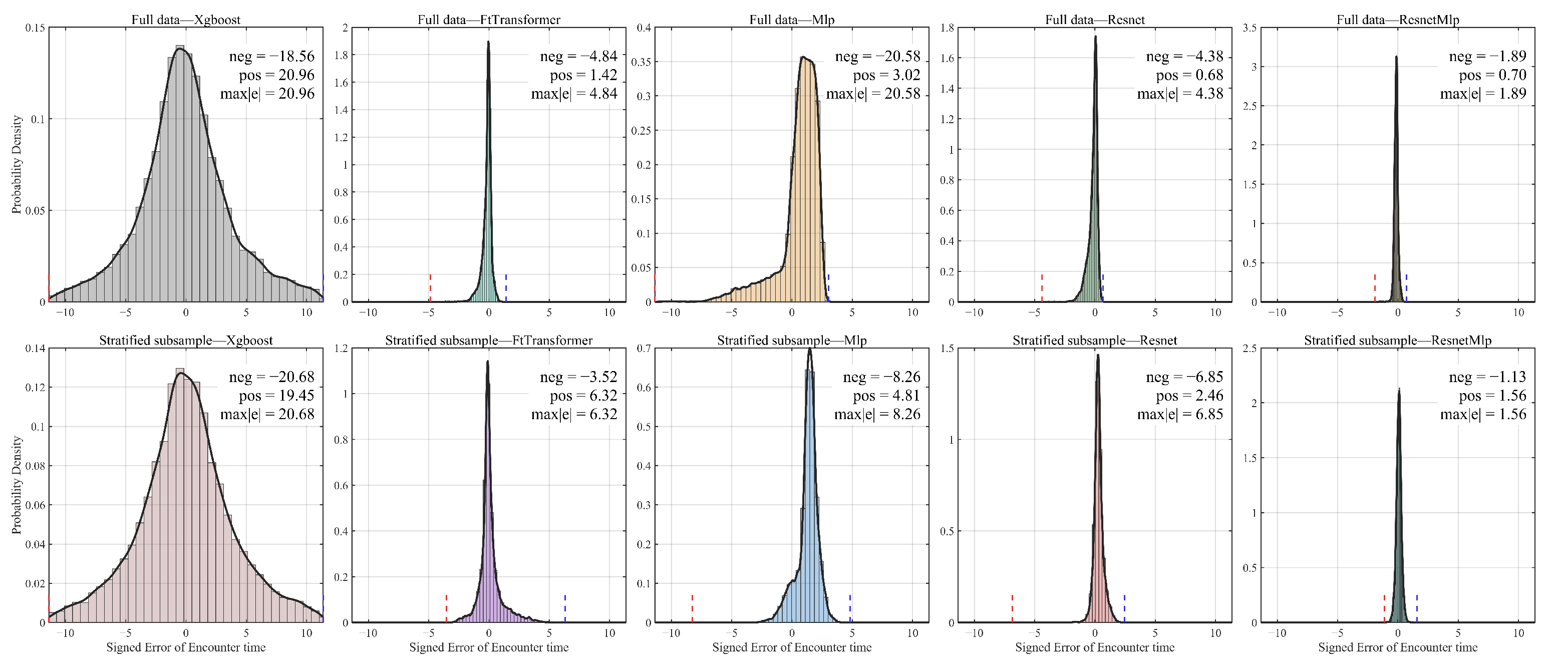
Table 4, Table 5, Table 6 and Table 7 compare the prediction results obtained using the full training dataset and the stratified training subset. For the encounter time, the prediction accuracy of ResNet-MLP is almost preserved after replacing the full training dataset with the stratified training subset. The MAE and RMSE increase only slightly, while the maximum error decreases from 1.8929 s to 1.5691 s. This indicates that the reduced stratified subset introduces only a small loss in average temporal accuracy and improves the worst-case time prediction error.

Table 4. Prediction results of $\widehat{t_{hit}}$ under different training settings.

Training Dataset	Model	MAE	RMSE	${\mathit{R}}^2$	MAX
Full training dataset	XGBoost	3.0197	4.1839	0.9910	20.9638
	FT-Transformer	0.2744	0.4314	0.9960	4.8408
	MLP	1.4477	3.6190	0.9980	20.5801
	ResNet	0.2848	0.4324	0.9990	4.3892
	ResNet-MLP	0.1726	0.2146	0.9990	1.8929
Stratified training subset	XGBoost	3.2316	4.4364	0.9902	20.6844
	FT-Transformer	0.5909	0.9514	0.9990	6.3276
	MLP	1.4193	1.5633	0.9980	8.2645
	ResNet	0.3840	0.2565	0.9990	6.8597
	ResNet-MLP	0.1775	0.2302	0.9990	1.5691

Table 5. Prediction results of $\widehat{\Delta x_{hit}}$ under different training settings.

Training Setting	Model	MAE	MSE	RMSE	${\mathit{R}}^2$	MAX	MBE
Full training dataset	XGBoost	1144.32	3,231,964.87	1797.76	0.9894	14,832.62	0.28
	FT-Transformer	124.56	84,841.55	291.27	0.9997	3279.69	−0.41
	MLP	631.12	724,684.39	851.28	0.9970	7056.86	0.07
	ResNet	92.29	15,451.25	124.30	0.9990	1105.40	0.97
	ResNet-MLP	45.53	3846.31	62.01	0.9990	874.02	0.02
Stratified training subset	XGBoost	1169.57	3,382,266.95	1839.09	0.9880	15,083.32	0.60
	FT-Transformer	190.64	134,115.58	366.21	0.9990	3448.39	−0.14
	MLP	340.64	236,698.66	486.51	0.9990	3003.06	−0.08
	ResNet	82.07	13,237.84	115.05	0.9990	2373.80	−0.21
	ResNet-MLP	67.92	8600.55	92.73	0.9990	890.55	0.001

Table 6. Prediction results of $\widehat{\Delta y_{hit}}$ under different training settings.

Training Setting	Model	MAE	MSE	RMSE	${\mathit{R}}^2$	MAX	MBE
Full training dataset	XGBoost	1010.82	2,245,272.41	1498.423	0.9930	10,828.98	0.53
	FT-Transformer	184.99	237,934.88	487.78	0.9993	5502.97	−0.41
	MLP	605.35	562,966.48	750.31	0.9980	6138.09	0.71
	ResNet	99.03	33,256.96	182.36	0.9990	3946.94	−0.98
	ResNet-MLP	72.79	29,337.85	171.28	0.9990	4131.33	0.91
Stratified training subset	XGBoost	1050.74	2,418,043.87	1555.00	0.9925	10,290.36	0.92
	FT-Transformer	234.64	253,264.90	503.25	0.9990	5617.91	−0.44
	MLP	343.22	219,360.20	468.35	0.9990	5543.28	−0.16
	ResNet	93.64	23,173.45	152.22	0.9990	3138.73	−0.28
	ResNet-MLP	60.44	7212.66	84.92	0.9990	767.46	−0.59

Table 7. Prediction results of $\widehat{\Delta z_{hit}}$ under different training settings.

Training Setting	Model	MAE	MSE	RMSE	${\mathit{R}}^2$	MAX	MBE
Full training dataset	XGBoost	1358.00	3,460,362.71	1860.20	0.9877	11,020.93	−0.99
	FT-Transformer	125.98	61,340.38	247.66	0.9998	2576.50	−0.73
	MLP	614.70	571,987.49	756.29	0.9980	3880.29	0.72
	ResNet	74.69	12,942.43	113.76	0.9970	945.89	0.24
	ResNet-MLP	67.14	8147.37	90.26	0.9990	795.47	0.73
Stratified training subset	XGBoost	1370.73	3,476,736.85	1864.60	0.9870	10,506.95	−0.78
	FT-Transformer	321.19	286,206.94	534.98	0.9990	4591.85	0.76
	MLP	239.43	135,311.43	367.84	0.9990	4414.50	−0.64
	ResNet	118.55	25,071.92	158.34	0.9990	2120.78	−0.10
	ResNet-MLP	65.33	7744.34	88.00	0.9990	672.90	0.15

For the x-component, the MAE and RMSE increase to some extent, indicating a certain loss of average accuracy in this direction. However, the maximum error changes only slightly, from 874.02 m to 890.55 m, suggesting that the worst-case x-direction error is still well controlled. For the y-component, the stratified subset brings a clear improvement. The MAE and RMSE are both reduced, and the maximum error is significantly reduced about 81.4%. For the z-component, the MAE and RMSE decrease slightly, and the maximum error is reduced by about 15.4%. These results show that the stratified subset can effectively suppress some large-error samples, especially in the y- and z-directions.

Overall, it still preserves the main prediction capability while using fewer training samples, and it improves the control of several extreme errors. This suggests that the geometry-stratified sampling strategy provides a more compact and spatially balanced training set.

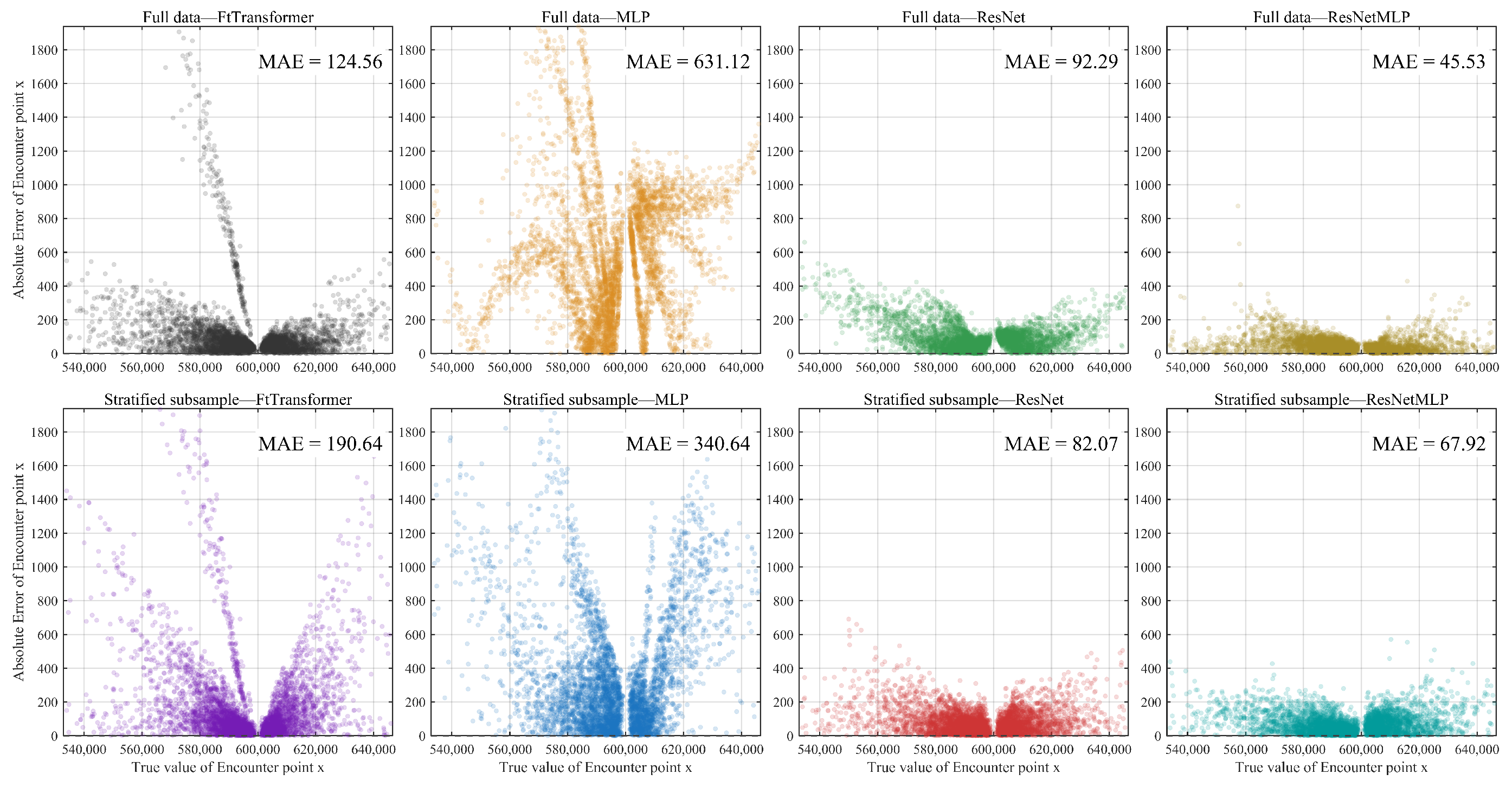
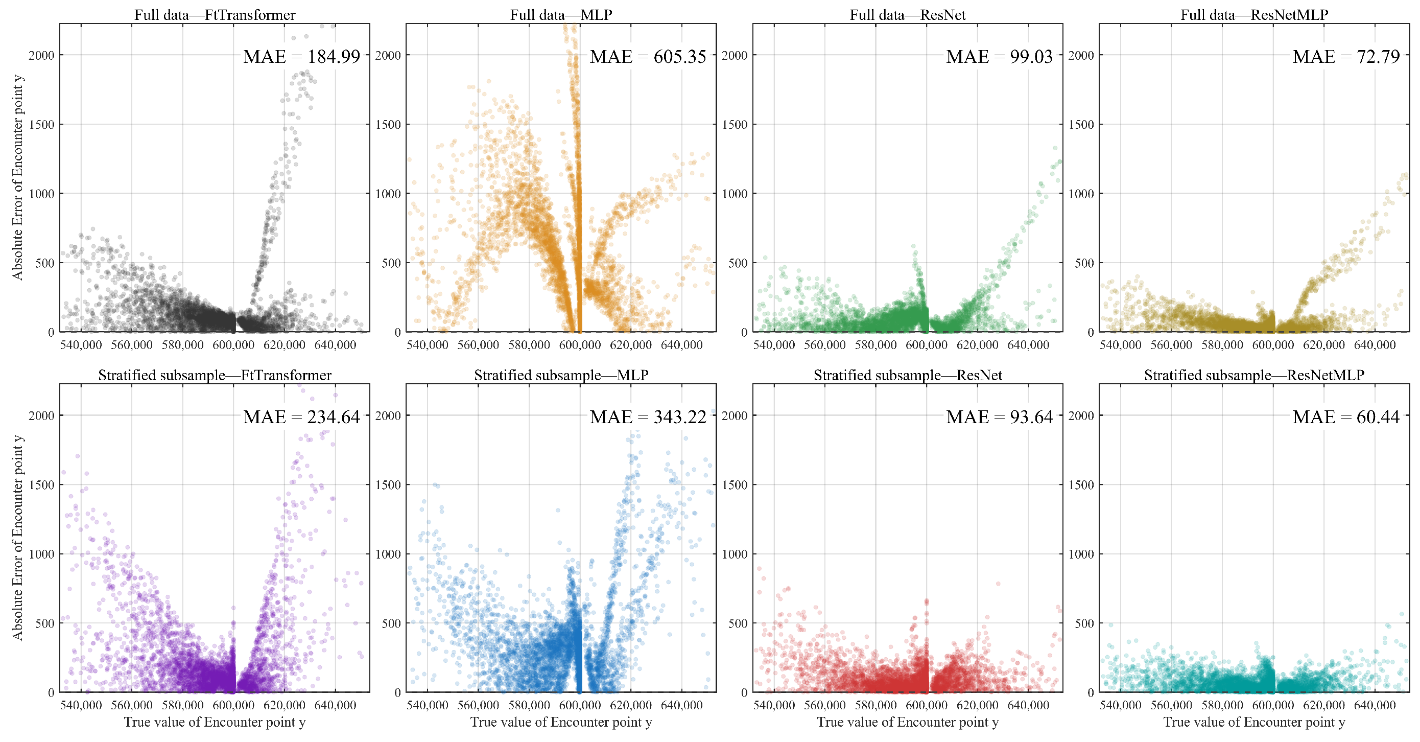
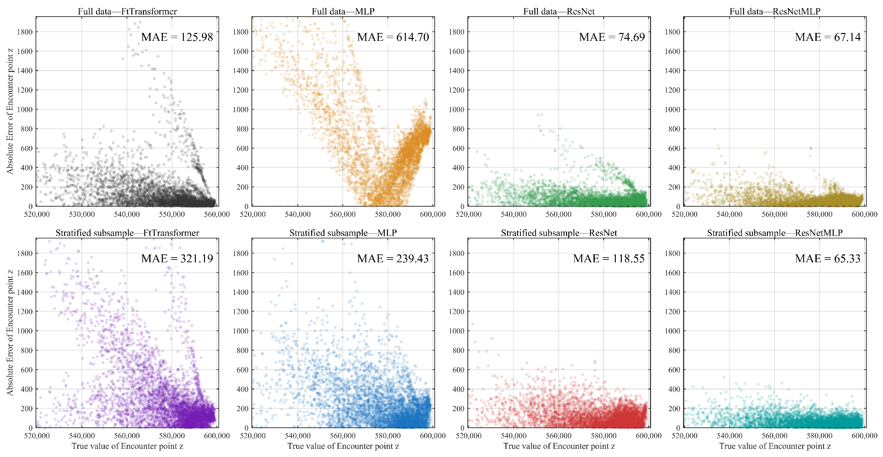
Figure 7 shows the absolute-error density distributions of the encounter time prediction, while Figure 8, Figure 9 and Figure 10 present the absolute-error scatter plots of the three encounter-point components. The density plot of the encounter time is consistent with the quantitative results in Table 4. ResNet-MLP has the most concentrated error distribution under both the full training dataset and the stratified training subset, indicating that most time-prediction errors are limited to a relatively small range. Compared with the full training dataset, the stratified training subset slightly increases the average time error but reduces the maximum time error, which shows that the reduced dataset still preserves stable time-prediction performance.

Figure 7. Absolute-error density plot of encounter time.

Figure 8. Absolute-error scatter plot of the x-component.

Figure 9. Absolute-error scatter plot of the y-component.

Figure 10. Absolute-error scatter plot of the z-component.

For the encounter-point components, the scatter plots further show the relationship between the true component values and the corresponding absolute errors. In the x-component, although the stratified training subset increases the MAE and RMSE of ResNet-MLP, the error points remain relatively concentrated and the maximum error changes only slightly. In the y- and z-components, the stratified training subset produces a narrower error band for ResNet-MLP and reduces the number of large-error samples, especially for the y-component. These visual results are consistent with the tabulated metrics and show that the stratified subset can retain the main prediction characteristics of the full dataset while using fewer training samples, and it provides a common training-data construction strategy for evaluating different surrogate regression models under the same physical prediction task.

6.2. $3D$ Euclidean Error Analysis

The encounter-point prediction task considered in this paper is intended to support subsequent penetration decision making. Therefore, the local error of a single coordinate component is not sufficient to evaluate the spatial prediction performance. To measure the overall deviation between the predicted and true encounter points, the three-dimensional Euclidean error is introduced as

$$e_{3d}=\sqrt{{(\Delta x-\Delta x_{pre})}^2+{(\Delta y-\Delta y_{pre})}^2+{(\Delta z-\Delta z_{pre})}^2}.$$

(43)

Table 8 presents the three-dimensional Euclidean error results. Compared with the full training dataset, the stratified training subset still maintains a similar level of three-dimensional MAE, indicating that the average spatial prediction accuracy is not significantly weakened after reducing the number of training samples. The large reduction of MAX shows that the geometry-stratified sampling strategy can effectively suppress extreme spatial errors and improve the stability of encounter-point prediction.

Table 8. $e_{3d}$ results under different training settings.

Training Setting	Model	MAE	RMSE	MAX
Full training dataset	XGBoost	3049.33	3690.01	15,052.53
	FT-Transformer	284.69	619.77	6571.87
	MLP	1213.76	1363.69	9472.59
	ResNet	177.38	248.30	4065.13
	ResNet-MLP	135.98	218.25	4287.84
Stratified training subset	XGBoost	2458.05	3045.82	15,540.79
	FT-Transformer	488.34	820.72	7409.15
	MLP	608.83	769.01	6592.02
	ResNet	198.72	247.96	3505.74
	ResNet-MLP	129.89	153.48	917.70

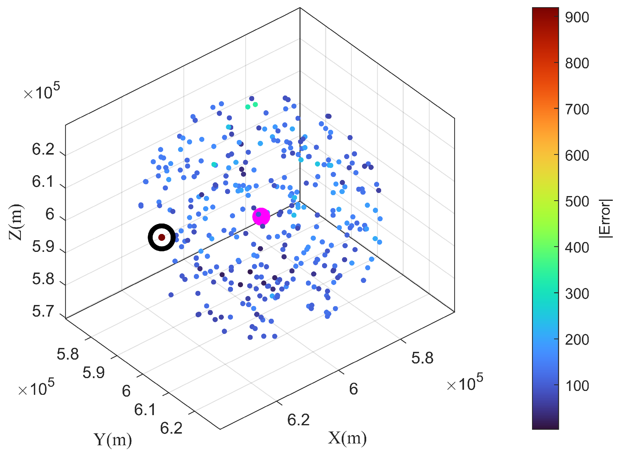
Figure 11 further shows the spatial distribution of the three-dimensional prediction error. Most samples are located in the low-error region, while only a small number of samples exhibit medium-to-high errors. The larger errors mainly appear near the outer boundary of the detectable region, where the prediction distance is longer and the geometric configuration is more difficult. This result is consistent with the bounded detectable-region assumption and suggests that the outer boundary is a relatively challenging region for prediction. In a future closed-loop application, the prediction can be repeatedly updated with newly observed relative states. However, the quantitative influence of such closed-loop updating on penetration maneuver performance still requires further validation.

Figure 11. Three-dimensional error distribution.

7. Generalization Performance Test

To further examine the spatial adaptability of the proposed relative-state prediction framework, a deployment-location generalization test is conducted. Different from the standard independent test set, this test changes the global deployment position of the maneuvering vehicle while keeping the ground target unchanged. Therefore, the test scenario is not a simple repetition of the original training condition but represents a shifted engagement configuration with a different maneuvering vehicle-to-target geometry.

Specifically, a representative deployment-location variation scenario is constructed by moving the maneuvering vehicle’s initial position away from the original training airspace. Under this changed deployment condition, a new generalization test dataset is generated. The approaching vehicle initial positions are regenerated around the shifted maneuvering vehicle within the bounded detectable threat region, and the feasible initial attitude set of the maneuvering vehicle is recalculated according to the same physical constraints. The trained ResNet-MLP predictor is then directly applied to this new dataset without retraining. In this way, the test is used to evaluate whether the learned mapping from the relative engagement state to the future encounter result can remain effective when the engagement airspace changes.

The results in Table 9 show that the proposed predictor maintains stable performance under the shifted deployment condition. After the deployment location is changed, the MAEs of the three encounter-point displacement components remain close to 100 m, and the MAE of the encounter time remains approximately 0.25 s. The corresponding $R^2$ values also remain high for all four outputs, indicating that the main mapping relationship learned from the original training domain is still preserved in the shifted engagement scenario.

Table 9. Prediction results under the deployment-location generalization test.

	MAE	MSE	RMSE	${\mathit{R}}^2$	MAX	MBE
$\widehat{\Delta x_{hit}}$	110.19	30,046.21	173.33	0.999	1480.57	0.20
$\widehat{\Delta y_{hit}}$	111.99	31,357.86	177.08	0.999	1678.80	0.10
$\widehat{\Delta z_{hit}}$	106.04	27,140.54	164.74	0.998	1667.03	0.23
$\widehat{t_{hit}}$	0.2474	0.11	0.3317	0.99	1.96	0.085

To further evaluate the overall spatial prediction performance, the three-dimensional Euclidean error of the encounter point is also analyzed. The results show that most spatial errors are concentrated within several hundred meters, with 90% of the samples below 450 m and 99% below 1 km. Considering that the predicted encounter point is used to provide spatial threat information for subsequent maneuver decision making rather than to achieve centimeter-level point coincidence, this level of spatial error remains acceptable for constructing a practical threat region and supporting avoidance-triggering decisions.

These results suggest that the proposed maneuvering vehicle-centered relative-state representation can reduce the dependence of the predictor on a fixed global coordinate frame. Although the absolute deployment position changes, the input features still describe the physically meaningful relative geometry between the maneuvering vehicle and the approaching vehicle. Therefore, the predictor can retain stable cross-deployment prediction performance within the considered bounded threat domain. In addition, the larger errors in the generalization test mainly appear near the outer region of the detectable domain, which is consistent with the previous three-dimensional error analysis. This indicates that the prediction difficulty is still mainly related to the relative engagement geometry and boundary-region characteristics rather than being dominated by the absolute spatial location of the engagement scenario.

Overall, the generalization test provides evidence that the proposed framework does not simply memorize the absolute spatial location of the training scenario but learns a relative-state mapping that can be transferred to a shifted deployment condition within the bounded detectable threat domain.

8. Robustness Test

In practical flight environments, radar measurements are inevitably affected by noise, which introduces errors into the detected position components of the approaching vehicle. To simulate this uncertainty, mutually independent bounded noise is added to the three relative-position features in the simulation data, with each component ranging from $[-50,50]$ m. This setting is used to represent the uncertainty introduced by sensors and tracking algorithms. Because the ResNet-MLP model achieved the best performance in the previous subsection and the other models failed to satisfy the accuracy requirement, the robustness test focuses on evaluating the prediction capability of the ResNet-MLP model trained with stratified uniform sampling on the noisy data.

The results in Table 10 show that the proposed model remains stable under bounded-error conditions. The overall evaluation metrics remain favorable, demonstrating that the method possesses good robustness capability.

Table 10. Prediction performance of the ResNet-MLP model under noisy conditions.

	MAE	MSE	RMSE	${\mathit{R}}^2$	MAX	MBE
$\widehat{\Delta x_{hit}}$	70.07	9180.31	95.81	0.998	979.80	1.12
$\widehat{\Delta y_{hit}}$	63.32	7955.70	89.19	0.999	774.05	0.58
$\widehat{\Delta z_{hit}}$	71.31	9235.30	96.10	0.999	721.08	0.20
$\widehat{t_{hit}}$	0.1996	0.0675	0.2598	0.999	1.6403	0.075

9. Conclusions

This paper focuses on the rapid prediction of the encounter point and encounter time in three-dimensional multi-vehicle interaction scenarios and proposes a physics-constrained relative-state prediction framework for penetration decision support. The proposed framework aims to address the spatial generalization problem of absolute-coordinate-based data-driven prediction methods, as well as the large sample scale and imbalanced sample distribution caused by an unconstrained prediction space.

By establishing a maneuvering vehicle-centered relative-state representation, the proposed framework reduces the dependence of the prediction model on a fixed global coordinate frame and a specific engagement airspace. A concentric double-spherical-shell detectable threat region is further constructed to constrain the originally unbounded prediction space into a finite region with clear physical meaning. In addition, a geometry-stratified sampling strategy combined with sample-weight correction is adopted to improve the balance of sample distribution under different distance layers and incoming directions.

On this basis, a ResNet-MLP joint regression model is employed as a fast online predictor to output the predicted encounter-point displacement and encounter-time information. Simulation results show that the stratified training subset, together with sample-weight correction, can reduce the required training data scale while maintaining prediction accuracy comparable to that of the full training dataset. The results also indicate that the proposed framework helps control the overall three-dimensional spatial error and suppress some local extreme prediction errors. The tests under deployment-location variations and bounded measurement disturbances further show that the predictor maintains stable performance within the considered engagement setting. In addition, the trained ResNet-MLP requires approximately 1.3–1.4 ms per prediction. As an auxiliary comparison, the simplified iterative predicted-hit-point method requires approximately 104–111 ms per prediction under the same computing environment, corresponding to an approximately 75–80-fold reduction in online computation time.

The proposed framework is mainly applicable to finite-threat-region, short-duration, constant-speed engagement scenarios with external information support, and it currently relies on fixed guidance laws and fixed guidance-parameter settings. Future work may extend the present framework to variable-speed dynamics, variable-thrust approaching vehicles, higher-fidelity six-degree-of-freedom models, and multiple guidance-law or guidance-parameter settings. In addition, high-fidelity simulation data or real flight-test data, if available, can be used for further validation or transfer adaptation. Future work may also integrate the predicted encounter point and encounter time with evasive decision making and online replanning techniques to build a closed-loop penetration framework with prediction-decision integration.