Fast Estimation of the Diffractive Loads on a Quadrotor UAV Following an Explosive Blast

Abstract

This work develops a tool to efficiently estimate the diffractive loads on a quadrotor uncrewed aerial vehicle (UAV) immediately following a nearby explosion. Existing models in the literature that predict the time history of wind velocity and the overpressure at a single distance from the blast are extended to model a moving blast wave that passes over the vehicle. The time-varying diffractive loads (i.e., due to the blast-induced pressure differential) are first modeled for a single sphere in a blast wave and then for a quadrotor approximated as a series of spheres connected by rods—one sphere for each of the four motors and one sphere for the central body. The overpressure and wind velocity models are compared with computational fluid dynamics (CFD) data. To illustrate the computational approach, a representative quadrotor model is perturbed by a blast from an initial hover flight condition in simulation. The rigid body dynamics are simulated over a short duration (ninety milliseconds) to determine the UAV’s state immediately after the explosion has concluded. The vehicle state history is predicted under the assumption of diffractive loads with a quadratic drag model and constant hover thrust.

1. Introduction

Small uncrewed aerial vehicles (UAVs) are frequently used in applications that support rescue intervention teams in hazardous environments [1], monitoring blasting activities on mountains [2] and in mines [3], and in military contexts [4]. Such operations expose UAVs to potential explosive blasts that may result in perturbations, flight instabilities, or damage to the UAV, making the modeling of their response to such events critical. The forces that act on the vehicle during a blast encounter can be categorized as diffractive, aerodynamic, or thrust loads. For strong and/or close-proximity blasts, the diffractive loads [5] on an object experiencing a blast can be much greater than the aerodynamic and thrust loads. The diffractive loads are a result of a spatially distributed time-varying blast pressure wave that passes over the vehicle’s body—while one side of the vehicle is experiencing higher static pressure, the other side experiences lower static pressure. This static pressure gradient results in net forces and moments that disturb the vehicle. This article develops a technique to quickly estimate these diffractive loads by approximating the vehicle using simple geometric shapes (i.e., spheres connected by rods) and performing fast numerical integrations of the static pressure field over the resulting rigid body. The new methodology developed provides a tool to support simulating blast response and control design for recovering from blasts.

1.1. Background and Related Work

Blasts produce a combination of pressure and air velocity disturbances that travel outward from the source. The pressure wave has spherical or cylindrical expansion with a monotonically decreasing propagation velocity converging to the speed of sound [6]. The Friedlander wave model [7] is often used as a model to describe the pressure over time at a distance from an explosion. Air velocity exhibits similar spreading with a sharp peak followed by a steep decrease to zero as distance increases and time progresses [8]. Scaled distance from the center of the blast is commonly used to parametrize blast characteristics in such models, by dividing the distance to the blast source by the cubed root of the mass of the explosive. In [9] an analytical model was developed describing how overpressure, temperature, and air velocity evolve during a blast. A survey of other blast models can be found in [6,10]. A model to predict the motion of a variety of objects due to a blast wave was studied in [5], finding that irregularly shaped objects can be approximated by a sphere—a concept which is exploited in this work. Sandia National Laboratories experimentally studied the blast characteristics required to cause catastrophic flight failure in a small UAV [11], concluding that overpressure values > 27 psi consistently destabilized the drone, possibly due to shock effects inducing sufficient resonance or damage to the internal inertial measurement unit (IMU). Overpressure effects from tank muzzle blasts on UAVs were also evaluated through experiments in [4]; however, in this case, the authors found that the effects on a drone flying 20 ft above the tank muzzle were negligible. The study of aircraft interaction with blasts is often conducted in the context of survivability analysis. For example, [12] provides a vulnerability assessment of combat aircraft to blast loading, and the work [13] conducted a damage assessment of an aircraft wing using finite element analysis. Finite element models can be used to evaluate UAV blast wave survivability by analyzing the force generated by a shock wave over time [14], but, similar to computational fluid dynamics (CFD) models, are computationally expensive for rapid prototype design and analysis.

1.2. Contributions and Article Organization

The main contributions of this work are (1) a model to approximate the blast’s spatiotemporal pressure distribution, referred to as the convected wave assumption, in the vicinity of the quadrotor, and (2) a computationally efficient technique to estimate the diffractive loads on the quadrotor by approximating the vehicle’s body as a set of spherical elements. CFD simulations were performed to illustrate that the proposed convected blast pressure and velocity field can be tuned to match higher-fidelity CFD data. Moreover, the proposed diffractive load estimator is illustrated for predicting loads over a representative quadrotor over which the forces and moments induced by the explosion are integrated with the equations of motion for a quadrotor. The simulation depends on several blast parameters (peak overpressure, wave propagation speed, positive phase duration, explosive mass, standoff distance, and relative blast angle) that can be readily adjusted to compare different blast conditions. For simulation purposes, simple aerodynamic and thrust force models are used to conceptually illustrate the working principle—modeling the aerodynamic and thrust loads variation experienced as a result of the blast is outside the scope of this article. The simulation framework is developed in Simulink, which facilitates model improvements (for example, alternative drag, thrust, control, or blast models can easily be integrated and tested).

The remainder of the article is organized as follows. Section 2 introduces the convected wave assumption that leads to an estimate of the pressure and velocity field over time near an object in a blast. Section 3 describes the approach to diffractive load estimation, analyzes the convected wave assumption, provides an illustrative example of the model applied to the motion of a sphere, and presents the extension to a quadrotor modeled as a set of spheres. Several comparisons of the convected wave assumptions and simulations of the loads and dynamic response of the quadrotor to a blast are presented in Section 4, including a sensitivity analysis. Section 5 describes the limitations of the proposed model. Section 6 concludes the article.

This article is a revised and expanded version of a conference paper [15]. This manuscript improves substantively with the addition of an expanded set of simulation results and more rigorous validation of the proposed models. The data and models used to generate the illustrations in this article can be found in the public GitHub repository https://github.com/robotics-uncc/quadBlastSim (accessed on 10 July 2026).

2. Blast Pressure and Velocity Field Modeling

This section describes an approach to estimate the diffractive loads on a quadrotor. We begin by first reviewing existing models of blast-induced pressure and velocity at a point. Next, a convected wave assumption is introduced, which allows extending these point-wise models to describe the time-varying blast pressure and velocity over an object.

2.1. Existing Models of Blast-Induced Pressure and Velocity at a Fixed Point

2.1.1. Blast-Induced Pressure Model

When a blast occurs, it induces a sudden change in pressure and air velocity in the surrounding environment, which ultimately drives the diffractive loads (due to asymmetric pressure on an object) and aerodynamic loads such as drag (due to the blast-induced air velocity). The Friedlander waveform is often used to describe the overpressure (i.e., differential pressure relative to ambient conditions) over time at a distance d from an explosion:

$$P\left(t\right)=P_s{e}^{-t/\tau }[1-(t/\tau )],$$

(1)

where $P_s$ is the peak overpressure and $\tau$ is the positive phase duration of the explosion [6,16]. Both parameters $P_s$ and $\tau$ depend on the distance from the blast. In (1), the blast is assumed to impinge on the point of interest at the initial time of $t=0$ (i.e., the time delay for the blast to reach the point of interest is not accounted for). The profile of the pressure wave is an instantaneous spike to $P_s$ followed by a decay to zero after $\tau$ seconds (this portion of the pressure response is referred to as the positive phase). For $t>\tau$ (referred to as the negative phase), a negative overpressure builds, dropping below ambient to create a partial vacuum. The vacuum effect can introduce diffractive loads that pull objects back towards the blast center. The negative phase reaches a minimum at $t=2\tau$ and then decays back towards zero asymptotically. At $t=8\tau$ the pressure is about $-0.00235P_s$ and has nearly returned to ambient conditions.

Various models have been proposed to estimate the parameters of peak overpressure $P_s$ (kPa) and positive phase duration $\tau$ (ms) that appear in (1). Typically, these parameters are assumed to depend on scaled distance, $S=d/\sqrt[3]{W}\left({\mathrm{m}/\mathrm{kg}}^{1/3}\right)$, or its constituent parts, distance from blast d (m), and explosive mass W (kg) [17]. The dependence on S introduces an equivalence in the pressure time-history that is experienced between different blasts (for example, an object a short distance away from a small blast may experience the same pressure fluctuation as an object a further distance away from a large blast generated by a greater explosive mass). In this work, the models presented by Sadovskiy [18] are used to capture the dependence of $P_s$ and $\tau$ on S:

$$P_s\left(d\right)=0.95{\displaystyle \frac{\sqrt[3]{W}}{d}}+3.9{\displaystyle \frac{\sqrt[3]{W^2}}{d^2}}+13{\displaystyle \frac{W}{d^3}}$$

(2)

and

$$\tau \left(d\right)=\sqrt[6]{W}\sqrt{d}.$$

(3)

The peak overpressure model provided by [18] outputs units of kg/cm², which must be converted to SI units, while the positive phase duration outputs units of ms. The coefficients used in this work model surface blasts, according to more recent work citing the same model [19]. Various models exist with slightly different coefficients for different scenarios of ground vs free-air blasts [19,20,21].

2.1.2. Blast-Induced Velocity Model

To represent the air velocity (wind) induced by the blast, the empirical model

$$V\left(T\right)=V_s{e}^{-\alpha T}(1-\beta T)+aln(1+\beta T),$$

(4)

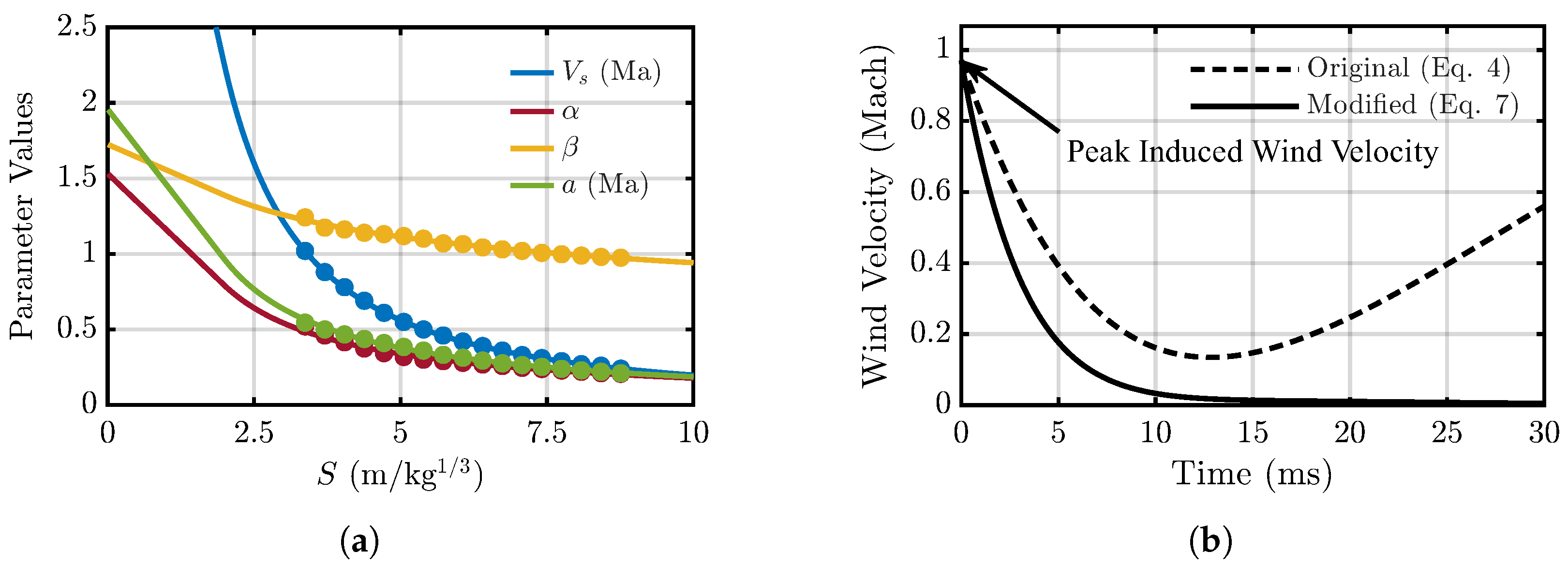
is proposed by Dewey in [8] where $V_s$ (Mach), a (Mach), $\alpha$, and $\beta$ are fitted parameters, and $T=k_{\mathrm{sound}}t/\sqrt[3]{W}$ is the scaled time where $k_{\mathrm{sound}}=343$ m/s is the ambient speed of sound and t is the time since the explosion. The parameters $\alpha$ and $\beta$ have units of inverse scaled time. A table of the parameters $(V_s,\alpha ,\beta ,a)$ and their dependence on S is available in [8] and is also reproduced in Figure 1a. An example of the wind velocity profile corresponding to (4) is shown as the dashed line in Figure 1b. The velocity profile (4) is similar to (1) in that it describes an instantaneous change at time $t=0$ followed by a decay. However, the velocity profile (4) grows without bound after the initial decay. This is due to the fact that (4) was developed by curve-fitting to experimental data which only spanned the initial period where wind velocity was monotonically decreasing [8]. To avoid the logarithmic increase in wind velocity following the initial decay, a modified wind velocity equation will be proposed in Section 2.3 (shown as the solid line in Figure 1b). Note also that the wind velocity profile plotted in Figure 1b utilizes a scaled distance of $S\approx 3.48{\mathrm{m}/\mathrm{kg}}^{1/3}$. Extrapolations may be used for values outside of the reported range as illustrated by the solid lines in Figure 1a.

2.2. Discussion of Parameter Selection

The above-described models by Sadovskiy [18] and Dewey [8] provide guidance on parameter selection in open-air blasts and can model a range of scaled distances (explosive mass and distances). The Sadovskiy models of peak overpressure and positive phase duration have a generally accepted applicable scaled distance range of $1{\mathrm{m}/\mathrm{kg}}^{1/3}$ to $15{\mathrm{m}/\mathrm{kg}}^{1/3}$ [19]. Additionally, the Sadovskiy models are only suitable for overpressures $>40P_0$, or ∼$4.053$ MPa at sea level [22]. The curve fitted parametric model of wind velocity provided by Dewey was published based on a scaled distance range of ∼$3.37{\mathrm{m}/\mathrm{kg}}^{1/3}$ to ∼$8.76{\mathrm{m}/\mathrm{kg}}^{1/3}$ and was fitted to data collected from explosions of T.N.T. charges ranging from ∼$13.6\mathrm{kg}$ to ∼90,718.5 kg. When comparing the predicted overpressure from Sadovskiy against experimental values obtained during experiments with a small UAV [11], the reported overpressure in [11] was approximately 2.9 times higher than predicted. This may be due, at least in part, to the fact that the blast in [11] occurred close to the ground. Reference [23] reports that a scale factor of two may apply for ground blast overpressure to account for ground reflections. However, depending on the energy absorption characteristics of the ground, this factor might be reduced by up to 20% [24]. The effect of ground reflections can also be modeled directly with CFD simulations by selecting the appropriate burst model [25]. Numerous other models exist that provide guidance on parameter selection for blasts based on computational studies and experiments. As we will later show, the model parameters can be tuned to match computational results.

2.3. Convected Blast Pressure and Velocity Field

Now consider the pressure and velocity field experienced by a small object placed in the vicinity of a blast. The classic models in the literature of pressure (1) and velocity (4) are intended for a specific distance d. To calculate diffractive loads, the pressure over the entire object is needed simultaneously and at each instant in time. To address this issue, we introduce a convected wave assumption that extends the Friedlander wave $P\left(t\right)$ valid at a single point to a related spatiotemporal pressure field valid over a range of points (and similarly for the blast-induced velocity). Recall that $P\left(t\right)$ is given by (1) and the parameters $P_s\left(d\right)$ and $\tau \left(d\right)$ are defined as functions of distance d and explosive mass W by (2) and (3). The convected wave assumptions are as follows:

1.

The blast originates at a point O and the blast-induced pressure and velocity experienced by an object with center point P located a distance $d_0$ from the blast center can be described in a blast reference frame $\mathcal{D}=\{O,{\mathit{e}}_1,{\mathit{e}}_2,{\mathit{e}}_3\}$ with the ${\mathit{e}}_1$ axis pointing in the direction of the ray joining points O and P.

2.

For a range of points $\overline{x}\in [d_0-ϵ,d_0+ϵ]$, along the ray joining O to P where $ϵ$ is a short distance over which the analysis is performed, the blast propagates as a plane wave with a spatially-varying velocity c in the ${\mathit{e}}_1$ direction so that the pressure and wind velocity is constant in each plane perpendicular to the wavefront’s velocity.

3.

The values of $P_s\left(\overline{x}\right)$, $\tau \left(\overline{x}\right)$, $c\left(\overline{x}\right)$ depend on the distance $\overline{x}\in [d_0-ϵ,d_0+ϵ]$.

4.

Without loss of generality, the blast can be assumed to begin at the initial time $t_{\mathrm{init}}=0$. The peak overpressure is then encountered at a point a distance $d_0$ away at time $t_0>t_{\mathrm{init}}$.

5.

The blast occurs in free air with no external interactions and the presence of the quadrotor does not alter the pressure or velocity field resulting from the blast.

6.

The forces and moments on a UAV in a blast can be decomposed into diffractive loads (i.e., due entirely to differential ambient pressure), aerodynamic loads (i.e., additional normal pressure fluctuations and shear stresses on the object’s surface due to fluid motion/wind), thrust loads, and weight. These loads are summed to give the net forces and moments.

The first and second assumptions that the blast is a plane wave are a simplification that is reasonable when the UAV being analyzed is small in size in comparison to the radius of a wavefront with spherical or cylindrical spreading. The blast propagation speed generally varies and this effect is captured, although the change in speed $c\left(\overline{x}\right)$ is relatively small over the range of distances $\overline{x}\in [d_0-ϵ,d_0+ϵ]$. This variation is determined through curve fitting (discussed later). Similarly, as stated in the third assumption, the parameters $P_s\left(\overline{x}\right)$ and $\tau \left(\overline{x}\right)$ vary slightly on this interval according to the parametric models in (2) and (3) and in Figure 1a. Additionally, this assumption holds when the perturbation induced by the blast is smaller than $ϵ$ so that the UAV does not leave the interval of distances analyzed. The fourth assumption defines the time at which we assume the blast to be experienced by the UAV. When a blast impinges on a UAV, a large overpressure spike occurs on the front face of the UAV (i.e., exceeding the free-field blast overpressure); however, this is not accounted for by the convected wave assumption. The fifth simplifying assumption ignores the reflections/interactions of the blast with the ground, nearby structures, and the quadrotor itself. The last assumption follows the precedent of other models, such as [26], that superimpose diffractive and aerodynamic loads. With the above assumptions, the following shifted waveform is proposed to represent the pressure at point P:

$$\begin{array}{c}\hfill P_0\left(t\right)=P_s\left(d_0\right)e^{-\Delta t/\tau \left(d_0\right)}[1-(\Delta t/\tau \left(d_0\right))]H(\Delta t),\end{array}$$

(5)

where $H(\Delta t)$ is a Heaviside function, $\Delta t=t-t_0$, and t is the elapsed time since the blast. The Heaviside function ensures the pressure is zero during the time it takes the blast wave to propagate to the object (i.e., $t_0$ is on the order of $d_0/c\left(\overline{x}\right)$ and more precisely $t_0={\int }_0^{d_0}{\displaystyle \frac{\mathrm{d}x}{c\left(x\right)}}$ when the variation of the propagation speed c is accounted for). Let $\overline{x}$ represent the distance from point O along the ${\mathit{e}}_1$ axis. As a result of the aforementioned assumptions, the pressure at a point $\overline{x}$ and time t is related to (5) by

$$\begin{array}{c}\hfill P(\overline{x},t)=P_0\left(t-{\displaystyle \frac{\overline{x}-d_0}{c\left(\overline{x}\right)}}\right),\end{array}$$

(6)

where $c\left(\overline{x}\right)$ is a propagation speed of the wavefront, which begins hypersonic, but quickly converges to the speed of sound. Equations (5) and (6) are the key assumptions that allow extending the single-distance Friedlander wave in the literature into a spatiotemporal disturbance field that the UAV is immersed in.

The convected wave assumption is also applied to the wind model (4). The wind model (4) is valid over a short time duration; however, for larger values of T the expression increases without bound. To ensure the limit approaches zero over time, this work proposes to modify (4) using an exponential decay term and the Heaviside function in the time domain:

$$\begin{array}{c}\hfill V_0\left(t\right)=\left(V_s{e}^{-\alpha T}\left(1-\beta T\right)+aln\left(1+\beta T\right)\right)H\left(T\right)e^{-T}.\end{array}$$

(7)

where $T=k_{\mathrm{sound}}\Delta t/\sqrt[3]{W}=k_{\mathrm{sound}}(t-t_0)/\sqrt[3]{W}$. The exponential decay term addresses the unbounded logarithmic growth, but it also attenuates the velocity decay more quickly at earlier times. Similar to (6), the velocity at a point $\overline{x}$ at time t is related to (7) by

$$\begin{array}{c}\hfill V(\overline{x},t)=V_0\left(t-{\displaystyle \frac{\overline{x}-d_0}{c\left(\overline{x}\right)}}\right).\end{array}$$

(8)

Together, (6) and (8) provide the pressure and velocity fields, respectively, around the vicinity of the UAV.

3. Fast Diffractive Load Estimation

This section presents a model to integrate the pressure field from the convected wave assumption over a single sphere and then a quadrotor approximated as a set of spheres.

3.1. Diffractive Load Estimation on a Stationary Spherical Object

Suppose that the sphere is located at a distance $d_0$ from the blast and the convected wave assumptions apply. Let $P_R({\theta }_B,{\varphi }_B,t)$ describe the pressure at a point on a sphere of radius R expressed using spherical coordinates in frame $\mathcal{D}$ where ${\theta }_B$ and ${\varphi }_B$ are the azimuth and polar angles of the blast, respectively. The azimuth angle ${\theta }_B$ is measured in the ${\mathit{e}}_1$–${\mathit{e}}_2$ plane and the polar angle ${\varphi }_B$ is measured from ${\mathit{e}}_3$. The pressure $P_R({\theta }_B,{\varphi }_B,t)$ can be obtained from (6) by substituting $\overline{x}=Rsin{\varphi }_{B}cos{\theta }_B+d_0$. The net force on the sphere is obtained by integrating the pressure over the entire surface

$$\begin{array}{c}\hfill \mathit{F}\left(t\right)=-{\int }_0^{2\pi }{\int }_0^{\pi }{P}_R({\theta }_B,{\varphi }_B,t)\widehat{\mathit{n}}({\theta }_B,{\varphi }_B)\mathrm{d}A\end{array}$$

(9)

where $\widehat{\mathit{n}}({\theta }_B,{\varphi }_B)={[sin{\varphi }_{B}cos{\theta }_B,sin{\varphi }_{B}sin{\theta }_B,cos{\varphi }_B]}^{\mathrm{T}}$ is a vector normal to the sphere’s surface (resolved in the $\mathcal{D}$ frame) and $\mathrm{d}A=R^{2}sin{\varphi }_B\mathrm{d}{\theta }_B\mathrm{d}{\varphi }_B$ is the area element in spherical coordinates. Due to the symmetry of the sphere, the force always points in the direction of the blast ray. Using Cartesian coordinates and recognizing that slices of the sphere in the ${\mathit{e}}_2$–${\mathit{e}}_3$ plane have constant pressure allows reducing (9) to a one-dimensional integral (and thus fast diffractive load estimation). Let $\gamma \in [0,\pi ]$ denote the angle (in a tilted plane) measured from the ${\mathit{e}}_1$ axis, so that a point on the sphere’s surface has axial position $\overline{x}=d_0+Rcos\gamma$. The locus of points on the sphere with constant pressure has constant $\gamma$ and sweeps out a cone shape. Thus, the pressure through the ${\mathit{e}}_2$–${\mathit{e}}_3$ slices is entirely determined by $\gamma$ and, due to symmetry, the net force must be in the ${\mathit{e}}_1$ direction (i.e., all other components integrate to zero). Let this pressure be denoted $P_{\mathrm{radial}}(\gamma ,t)$. Then the axial component is obtained by collecting the ring of surface area $2\pi R^{2}sin\gamma \mathrm{d}\gamma$ at each angle $\gamma$, giving the signed axial force

$$\begin{array}{c}\hfill F_0\left(t\right)=-{\int }_0^{\pi }{P}_{\mathrm{radial}}(\gamma ,t)cos\gamma \left(2\pi R^{2}sin\gamma \right)\mathrm{d}\gamma ,\end{array}$$

(10)

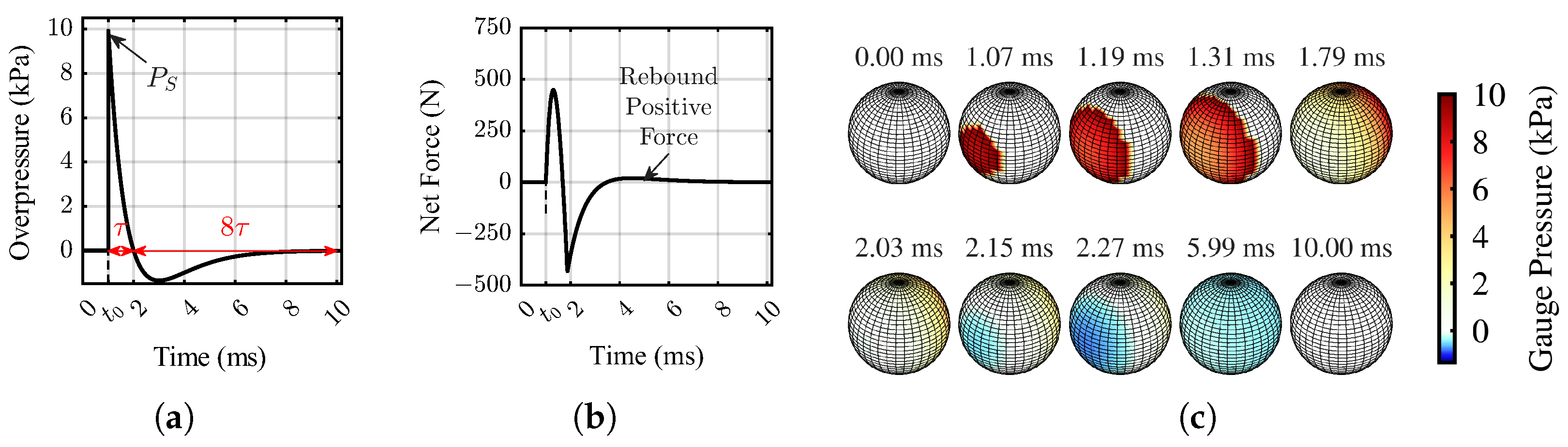
such that $\mathit{F}\left(t\right)=F_0\left(t\right){\mathit{e}}_1$ where $P_{\mathrm{radial}}(\gamma ,t)=P(d_0+Rcos\gamma ,t)$ is obtained from (6). Equation (10) is evaluated numerically using trapezoidal integration. Figure 2a shows a pressure-over-time profile given by a Friedlander wave with a peak overpressure $P_s=10$ kPa, time constant $\tau =1$ ms, and a constant propagation speed $c=343$ m/s. Integrating the pressure over the surface of the sphere provides the net force distribution shown in Figure 2b. Over time, the sphere experiences diffractive loads both towards and away from the blast center due to the pressure differential caused by the size of the body and the positive and negative phases of the Friedlander wave model.

3.2. Analysis of the Convected Wave Assumption

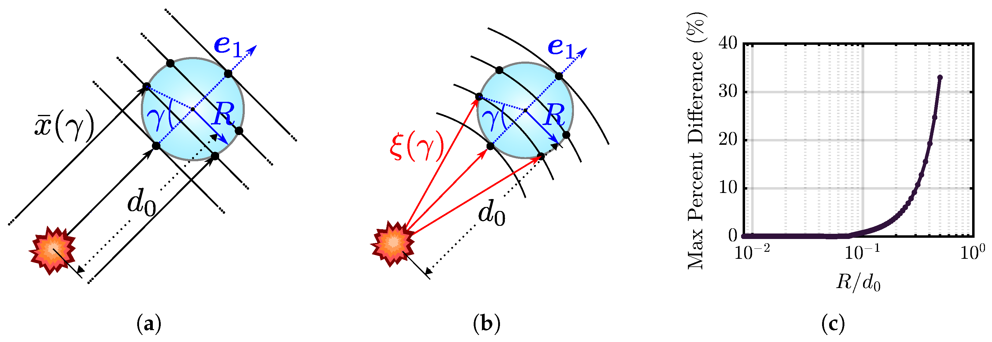
A comparison study was conducted to quantify the difference between using a simplified planar convected-wave assumption and a more accurate spherical convected-wave assumption. Using the planar wave assumption shown in Figure 3a, the blast rays are assumed to be parallel, modeling the blast propagation as a plane traveling through the sphere. Using the radial wave assumption shown in Figure 3b, let $\xi \left(\gamma \right)=\sqrt{{(d_0+Rcos\gamma )}^2+{(Rsin\gamma )}^2}$ denote the true radial distance to the surface of the modeled sphere.

Figure 3c shows the percent difference of the peak blast force between the two spreading assumptions for various standoff distances of a representative sphere of radius 0.25 m. An explosive mass of 10 kg, positive phase duration of 6 ms and constant propagation speed of 343 m/s was used for this comparison. The abscissa in Figure 3c is a unitless parameter defined as the radius of the sphere divided by the standoff distances to easily determine the applicability of the planar wave approach for a generalized range of representative sphere radii and standoff distances. At $R/d_0\approx 0.1$, the percent difference begins to diverge between the two models, indicating that the planar wave spreading assumption is only valid when the standoff distance of the blast is at least 10 times the size of the object that is modeled. Using the standard definitions of the geometric properties of a circular arc, this ratio can be written in terms of sagitta s, or the distance from the midpoint of an arc to the midpoint of a chord of given length l. Using the diameter of the sphere in the blast as the chord length (i.e., $R=l/2$), and the standoff distance from the blast as the radius of the circular arc gives:

$$\begin{array}{cc}\hfill d_0^2& =R^2+{(d_0-s)}^2.\hfill \end{array}$$

(11)

Rearranging Equation (11) for $s/R$ and evaluating gives 0.0501, indicating that the ratio of the depth of the blast wave, which encompasses the sphere, is only ∼5% as long as the radius of the sphere. For $R/d_0\ge 0.1$, the error increases asymptotically because the sagitta grows to engulf more of the sphere, making the planar wave assumption invalid at close standoff distances.

3.3. Illustrative Example of a Single Sphere

To highlight how the overpressure and induced air speed of a blast may affect the motion of a sphere, a simple example is constructed using 1-dimensional dynamics affected by the force from the pressure wave and the drag from the resultant wind. Define the equation of motion of a sphere as

$$\dot{\mathit{z}}=\left[\begin{array}{c}{\dot{z}}_1\\ {\dot{z}}_2\end{array}\right]=\left[\begin{array}{c}{z}_2\\ {\displaystyle \frac{F_0\left(t\right)}{m}}+{\displaystyle \frac{F_D}{m}}\end{array}\right],$$

(12)

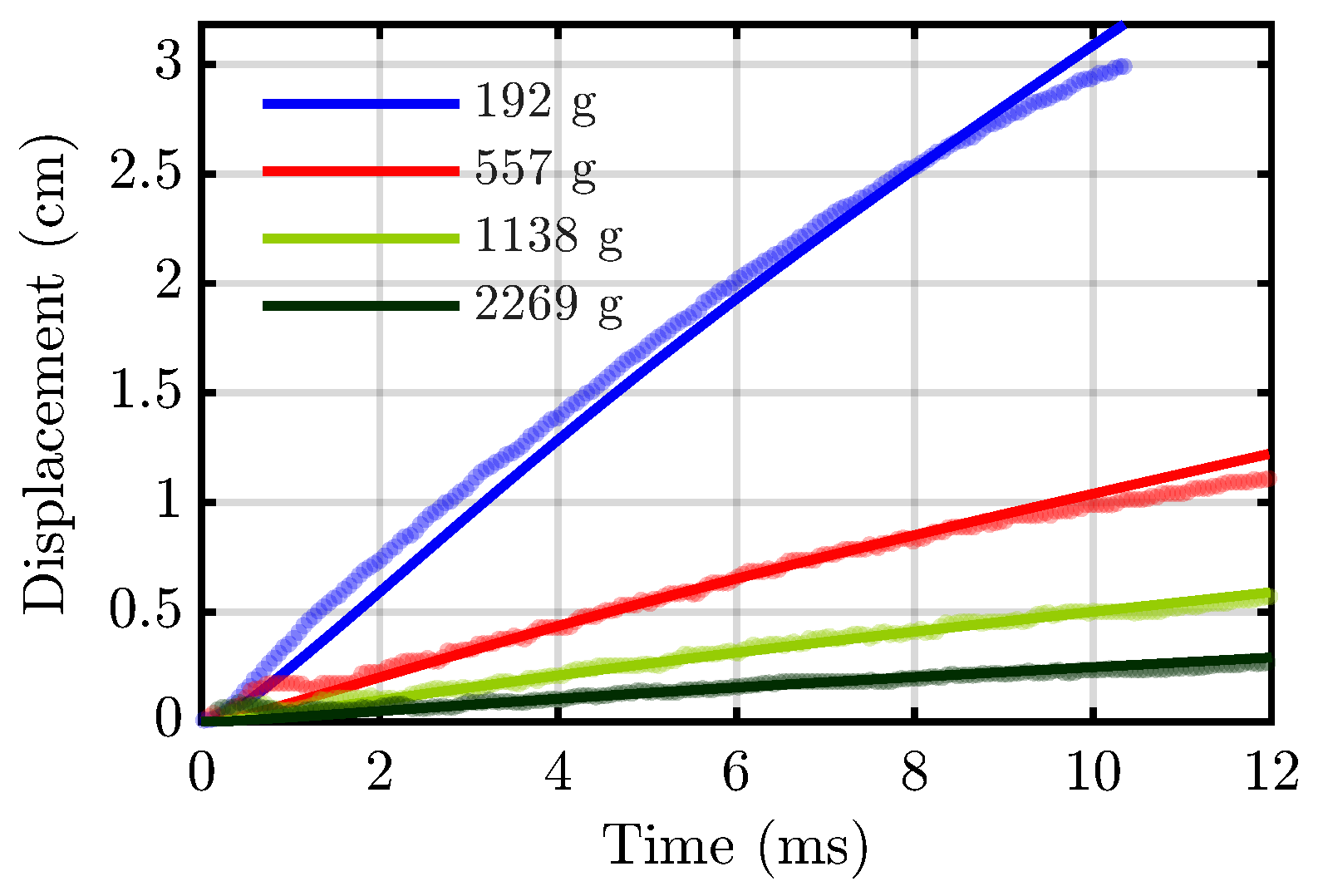
where $F_D=-{\displaystyle \frac{1}{2}}\rho C_{D}A\left|v^{\mathrm{rel}}\right|v^{\mathrm{rel}}$ is the drag force, $v^{\mathrm{rel}}=z_2-V_0\left(T\right)$ is the relative velocity of the sphere, $V_0\left(T\right)$ is the velocity at the sphere center’s initial position given by (7) (wherein scaled time T is related to time t), $A=\pi R^2$ is the projected two-dimensional frontal area for the sphere, $z_1$ is the position of the sphere, $z_2$ is its velocity, m (kg) is its mass, $\rho \left({\mathrm{kg}/\mathrm{m}}^3\right)$ is the air density, and $C_D$ is a drag coefficient. In [27], a shock-tube experiment was conducted to investigate the motion of spheres in a blast. Here, the blast and sphere parameters from [27] are replicated for validation of the presented blast models, where $P_s=125$ kPa, $\tau =6$ ms, $R=0.143$ m, a constant propagation speed $c=343$ m/s, and various sphere masses m shown as different colors corresponding to the colors shown in the original article.

Figure 4 illustrates the movement of a sphere initially at rest using the standoff distances $d_0$, explosive masses W, and drag coefficients $C_D$ shown in

Table 1. Optimized parameters for [27] M-Series spheres.

Sphere	Mass (g)	W (kg)	${\mathit{d}}_0$ (m)	${\mathit{C}}_{\mathit{D}}$
1	192	14.97	10.12	0.523
2	557	14.96	10.13	0.488
3	1138	14.96	10.14	0.480
4	2269	14.96	10.14	0.479

. The light colored data shown in Figure 4 was digitized from the unscaled data shown in Figure 5 of [27] using an online plot digitizer [28]. The radius of the M-Series sphere is left constant at $0.0715$ m, with the mass of the sphere set based on the numbered IDs in [27], as listed in Table 1. The models described in Section 2 were used to perturb the spheres with an explosion traveling in the ${\mathit{e}}_1$ direction, on a short timescale of 12 ms to match the original data. General parameters such as peak overpressure and positive phase duration were matched to the shockwave experiments in [27], where $P_s=\mathrm{125,000}$ Pa, and $\tau =6$ ms. The explosive mass, standoff distance, and drag coefficients were used as decision variables in a sequential quadratic programming (SQP) based optimization in MATLAB [29] to find the blast parameters which best minimized the error between the digitized data and the model output. The optimized values of explosive mass of ∼15 kg with a standoff distance of ∼10 m produce overpressure and positive phase durations which closely match the shock-tube conditions reported in the referenced experiments. The optimized results also show a fairly consistent drag coefficient, with an average value of ∼0.4925, which closely matches the drag coefficient for a sphere reported in the literature of $C_D=0.47$ [30].

3.4. Fast Estimation of the Diffractive Loads on a Quadrotor UAV

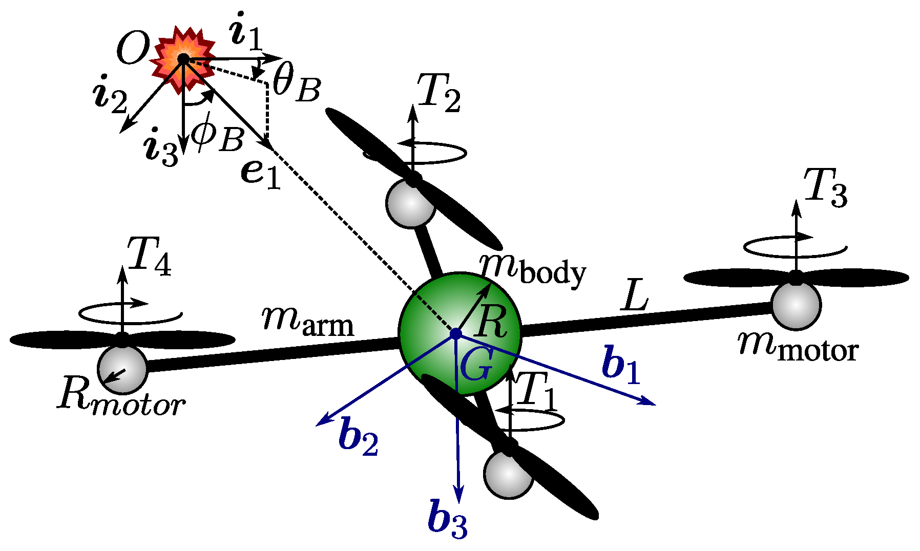
This section introduces a quadrotor model consisting of four spherical motors, four thin-rod arms, and a spherical central body as shown in Figure 5. The diffractive pressure loads over each of the spherical components are modeled independently to approximately capture the effect of the explosion that impinges non-uniformly on the quadrotor.

Let $\mathcal{I}=\{O,{\mathit{i}}_1,{\mathit{i}}_2,{\mathit{i}}_3\}$ denote a fixed inertial Cartesian reference frame in standard North-East-Down orientation, and let $\mathcal{B}=\{G,{\mathit{b}}_1,{\mathit{b}}_2,{\mathit{b}}_3\}$ denote a body-fixed reference frame with origin at the center of mass point G of the vehicle. Let $\mathit{x}={[x,y,z]}^{\mathrm{T}}$ and $\mathit{v}={[\dot{x},\dot{y},\dot{z}]}^{\mathrm{T}}$ denote the inertial position and velocity of G, respectively, resolved along the components of $\mathcal{I}$. Let $\mathsf{\Theta }={\left[\varphi ,\theta ,\psi \right]}^{\mathrm{T}}$ be a vector of roll, pitch, and yaw angles, respectively. The vector $\mathsf{\Omega }={[p,q,r]}^{\mathrm{T}}$ is the angular rotation rate of the body frame with respect to the inertial frame, resolved in body frame unit vectors. The standard 3-2-1 Euler angle sequence rotation matrix ${\mathit{R}}_{\mathcal{B}}^{\mathcal{I}}\left(\mathsf{\Theta }\right)$ relates reference frame $\mathcal{B}$ to $\mathcal{I}$.

The methodology of Section 2.3 can be extended to consider the effect of the blast forces on the individual elements of the quadrotor. Let the source of the blast point be $\mathit{b}$ in an inertial frame. Assume that the explosion propagates toward the vehicle along $\mathit{d}=\mathit{x}-\mathit{b}$, with unit vector $\widehat{\mathit{d}}=\mathit{d}/\parallel \mathit{d}\parallel$ coinciding with the direction of the ${\mathit{e}}_1$ unit vector in frame $\mathcal{D}$ introduced earlier. The position of the ith motor sphere in the vehicle’s body frame is

$$\begin{array}{c}\hfill {\mathit{r}}_{\mathrm{motor},i/G}=(R+L)(cos{\zeta }_i{\mathit{b}}_1+sin{\zeta }_i{\mathit{b}}_2)\end{array}$$

(13)

for $i=1,\dots ,4$ where ${\zeta }_1=\pi /4$, ${\zeta }_2=5\pi /4$, ${\zeta }_3=7\pi /4$ and ${\zeta }_4=3\pi /4$ since the quadrotor is a symmetric “X” configuration (nominally flies forward with motors 1 and 3 in front). The index of the first motor to experience the explosion is

$$\begin{array}{c}\hfill i^{\ast }={\mathrm{argmin}}_{i\in \left\{1,2,3,4\right\}}\langle {\mathit{r}}_{\mathrm{motor},i/G},{\mathit{R}}_{\mathcal{I}}^{\mathcal{B}}\widehat{\mathit{d}}\rangle ,\end{array}$$

(14)

where $\langle ·,·\rangle$ is the inner product. Let $t_0$ denote the time at which the blast impacts this first motor. Equation (5) describes the Friedlander wave pressure referenced to this point in space, which is a distance $d_0$ from the origin. Assuming no motion or rotation of the UAV platform, the time to impact the remaining three motors would be

$$\begin{array}{c}\hfill t_i=t_0+{\displaystyle \frac{1}{c}}\langle {\mathit{r}}_{\mathrm{motor},i/G}-{\mathit{r}}_{\mathrm{motor},i^{\ast }/G},{\mathit{R}}_{\mathcal{I}}^{\mathcal{B}}\widehat{\mathit{d}}\rangle \end{array}$$

(15)

for $i\in \{1,2,3,4\}\setminus i^{\ast }$.

The forces across each motor along the direction $\widehat{\mathit{d}}$ and the force across each motor over time are computed from (6) and an appropriate modification of (9) to consider the spatial separation of the motors relative to the reference point $d_0$. Let ${\mathit{F}}_{\mathrm{motor},i}^{\mathrm{blast}}\left({\mathit{x}}_i,\mathsf{\Theta },t;r\right)$ denote a general expression for the blast force computed for motor i at an inertial position ${\mathit{x}}_i=\mathit{x}+{\mathit{r}}_{\mathrm{motor},i/G}$, assuming a spherical motor with radius $R_{\mathrm{motor}}$. Similarly, let ${\mathit{F}}_{\mathrm{body}}^{\mathrm{blast}}(\mathit{x},\mathsf{\Theta },t;R)$ denote a general expression for the blast force computed for the body of the UAV, at its inertial location $\mathit{x}$ assuming a radius R. The blast forces are computed in the $\mathcal{D}$ frame and must be rotated to the $\mathcal{I}$ frame. The net force on the UAV expressed in the inertial frame is the sum of all five blast forces across the motors and central body

$$\begin{array}{c}\hfill {\mathit{F}}^{\mathrm{blast}}(\mathit{x},\mathsf{\Theta },t)={\mathit{R}}_{\mathcal{D}}^{\mathcal{I}}{\mathit{F}}_{\mathrm{body}}^{\mathrm{blast}}(\mathit{x},\mathsf{\Theta },t;R)+{\displaystyle \sum _{i=1}^4}{\mathit{R}}_{\mathcal{D}}^{\mathcal{I}}{\mathit{F}}_{\mathrm{motor},i}^{\mathrm{blast}}\left({\mathit{x}}_i,\mathsf{\Theta },t;R_{\mathrm{motor}}\right).\end{array}$$

(16)

The net moment in the body frame is the resultant of the four motors

$$\begin{array}{c}\hfill {\mathit{M}}^{\mathrm{blast}}(\mathit{x},\mathsf{\Theta },t)={\displaystyle \sum _{i=1}^4}{\mathit{r}}_{\mathrm{motor},i/G}\times {\mathit{R}}_{\mathcal{D}}^{\mathcal{B}}{\mathit{F}}_{\mathrm{motor},i}^{\mathrm{blast}}\left({\mathit{x}}_i,\mathsf{\Theta },t;R_{\mathrm{motor}}\right)\end{array}$$

(17)

with no moment generated from the central body.

3.5. Extension to a Dynamic Model with Drag, Weight, and Thrust Forces and Moments

The Newton-Euler equations of motion of a quadrotor are used, with translational and rotational kinematics

$$\begin{array}{cc}\hfill \dot{\mathit{x}}& =\mathit{v}\hfill \end{array}$$

(18)

$$\begin{array}{cc}\hfill {\dot{\mathit{R}}}_{\mathcal{B}}^{\mathcal{I}}& ={\mathit{R}}_{\mathcal{B}}^{\mathcal{I}}\widehat{\mathsf{\Omega }},\hfill \end{array}$$

(19)

and dynamics

$$\begin{array}{cc}\hfill m\dot{\mathit{v}}& ={\mathit{F}}_{\mathrm{net}}^{\mathcal{I}}\hfill \end{array}$$

(20)

$$\begin{array}{cc}\hfill \mathit{I}\dot{\mathsf{\Omega }}+\mathsf{\Omega }\times \mathit{I}\mathsf{\Omega }& ={\mathit{M}}_{\mathrm{net}}^{\mathcal{B}},\hfill \end{array}$$

(21)

where m is the system mass, $\mathit{I}$ is the system inertia, and the hat operator $\left(\widehat{·}\right)$ defines the skew symmetric matrix relating components of the angular velocity vector $\mathsf{\Omega }$. The sum of forces, resolved into inertial-frame components, is

$$\begin{array}{c}\hfill {\mathit{F}}_{\mathrm{net}}^{\mathcal{I}}={\mathit{F}}^{\mathrm{blast}}(\mathit{x},\mathsf{\Theta },t)+{\mathit{F}}^{\mathrm{drag}}(\mathit{x},\mathsf{\Theta },t)+{\mathit{F}}^{\mathrm{thrust}}\left(\mathsf{\Theta }\right)+mg{\mathit{i}}_3.\end{array}$$

(22)

Similarly, the sum of moments is given in the body frame as

$$\begin{array}{c}\hfill {\mathit{M}}_{\mathrm{net}}^{\mathcal{B}}={\mathit{M}}^{\mathrm{blast}}(\mathit{x},\mathsf{\Theta },t)+{\mathit{M}}^{\mathrm{drag}}(\mathit{x},\mathsf{\Theta },t)+{\mathit{M}}^{\mathrm{thrust}}.\end{array}$$

(23)

The total mass of the system is $m=4m_{\mathrm{motor}}+4m_{\mathrm{arm}}+m_{\mathrm{body}}$. The motor arms have length L (taken as the distance from the center of the body-to-motor spheres), the motors are spheres with radius r, and the center body is a sphere of radius R. For this chosen configuration the total rigid body inertia is $\mathit{I}={\mathit{I}}_{\mathrm{body}}+{\mathit{I}}_{\mathrm{arms}}+{\mathit{I}}_{\mathrm{motors}}$ where ${\mathit{I}}_{\mathrm{body}}={\displaystyle \frac{2}{5}}{m}_{\mathrm{body}}{R}^2{\mathbf{1}}_{3\times 3}$, ${\mathit{I}}_{\mathrm{arms}}=m_{\mathrm{arm}}\mathrm{diag}(\kappa ,\kappa ,2\kappa )$ where $\kappa =(L^2/6)+2{(L/2+R)}^2$, and ${\mathit{I}}_{\mathrm{motors}}=m_{\mathrm{motor}}\mathrm{diag}\left(\lambda ,\lambda ,2\lambda \right)$ where $\lambda =2{(L+R_{\mathrm{motor}})}^2$. Although the motors are modeled as spheres with radius $R_{\mathrm{motor}}$, they are simplified as point masses for the purposes of inertia calculation. The forces on the arms are ignored.

Based on (8), an explosion induces a spatially and time-varying wind denoted $\mathit{w}(\mathit{x},t)$ that, when coupled with the inertial translational and rotational velocity, generates non-uniform local flow-relative velocities over the length of the quadrotor. A quadratic drag model with a constant drag coefficient is assumed. The inertial velocity of the body is $\mathit{v}$, and for each motor

$$\begin{array}{c}\hfill {\mathit{v}}_{\mathrm{motor},i}=\mathit{v}+{\mathit{R}}_{\mathcal{B}}^{\mathcal{I}}\left(\mathsf{\Omega }\times {\mathit{r}}_{\mathrm{motor},i/G}\right).\end{array}$$

(24)

The local wind velocity at the body is $\mathit{w}(\mathit{x},t)$, and at each motor

$$\begin{array}{c}\hfill {\mathit{w}}_{\mathrm{motor},i}=\mathit{w}(\mathit{x}+{\mathit{R}}_{\mathcal{B}}^{\mathcal{I}}{\mathit{r}}_{\mathrm{motor},i/G},t).\end{array}$$

(25)

The flow-relative velocities are then given at the body as ${\mathit{v}}^{\mathrm{rel}}=\mathit{v}-\mathit{w}$ and each motor as ${\mathit{v}}_{\mathrm{motor},i/G}^{\mathrm{rel}}={\mathit{v}}_{\mathrm{motor},i/G}-{\mathit{w}}_{\mathrm{motor},i/G}$. The total drag force on the UAV is

$$\begin{array}{c}\hfill {\mathit{F}}^{\mathrm{drag}}(\mathit{x},\mathsf{\Theta },t)={\mathit{F}}_{D,\mathrm{body}}+{\displaystyle \sum _{i=1}^4}{\mathit{F}}_{D,\mathrm{motor},i}\end{array}$$

(26)

where each drag force has the form ${\mathit{F}}_D=-{\displaystyle \frac{1}{2}}\rho C_{D}A\left|{\mathit{v}}^{\mathrm{rel}}\right|{\mathit{v}}^{\mathrm{rel}}$ where $\rho$ is the air density, $C_D$ is the drag coefficient, A is a reference area, and ${\mathit{v}}^{\mathrm{rel}}$ is the flow-relative velocity with each of the coefficients specified for the different components and using the corresponding flow-relative velocities. The moment due to drag is ${\mathit{M}}^{\mathrm{drag}}(\mathit{x},\mathsf{\Theta },t)={\sum }_{i=1}^4{\mathit{r}}_{\mathrm{motor},i/G}\times {\mathit{R}}_{\mathcal{I}}^{\mathcal{B}}{\mathit{F}}_{D,\mathrm{motor},i}$.

The weight of the quadrotor acts through the center of mass with a force $mg{\mathit{i}}_3$, and creates no moment. The thrust forces are expressed as ${\mathit{F}}_{\mathrm{motor},i}^{\mathrm{thrust}}=-T_i{\mathit{b}}_3$ where $T_i\ge 0$ is the thrust magnitude generated by each motor $i=1,2,3,4$ and acts at each motor position. The net thrust in the inertial frame is ${\mathit{F}}^{\mathrm{thrust}}\left(\mathsf{\Theta }\right)={\mathit{R}}_{\mathcal{B}}^{\mathcal{I}}{\sum }_{i=1}^4{\mathit{F}}_{\mathrm{motor},i}^{\mathrm{thrust}}$, and the thrust-induced moment in the body frame is ${\mathit{M}}^{\mathrm{thrust}}={\sum }_{i=1}^4{\mathit{r}}_{\mathrm{motor},i/G}\times {\mathit{F}}_{\mathrm{motor},i}^{\mathrm{thrust}}$. The simple models of thrust and drag adopted in this paper support the prediction of a quadrotor’s response to the blast and can be refined in future work, as suggested in Section 5, to improve the accuracy of the simulation.

4. Simulation Results

This section presents simulation results and comparisons that illustrate the blast modeling assumptions and quadrotor diffractive load estimation:

• Section 4.1 presents a computational fluid dynamics (CFD) simulation of an explosive blast event (without a quadrotor in the blast field). The resulting overpressure and air velocity fields are compared with the convected wave assumption.
• Section 4.2 describes a Simulink model that incorporates the diffractive load estimation approach to predict the terminal state of the quadrotor after the blast has passed.
• Section 4.3 describes a sensitivity study which analyzes the effects of using a range of constant drag coefficients and constant air density values to determine the sensitivity of the presented framework to changes in aerodynamic constants.

4.1. Computational Fluid Dynamics (CFD) Model Validation

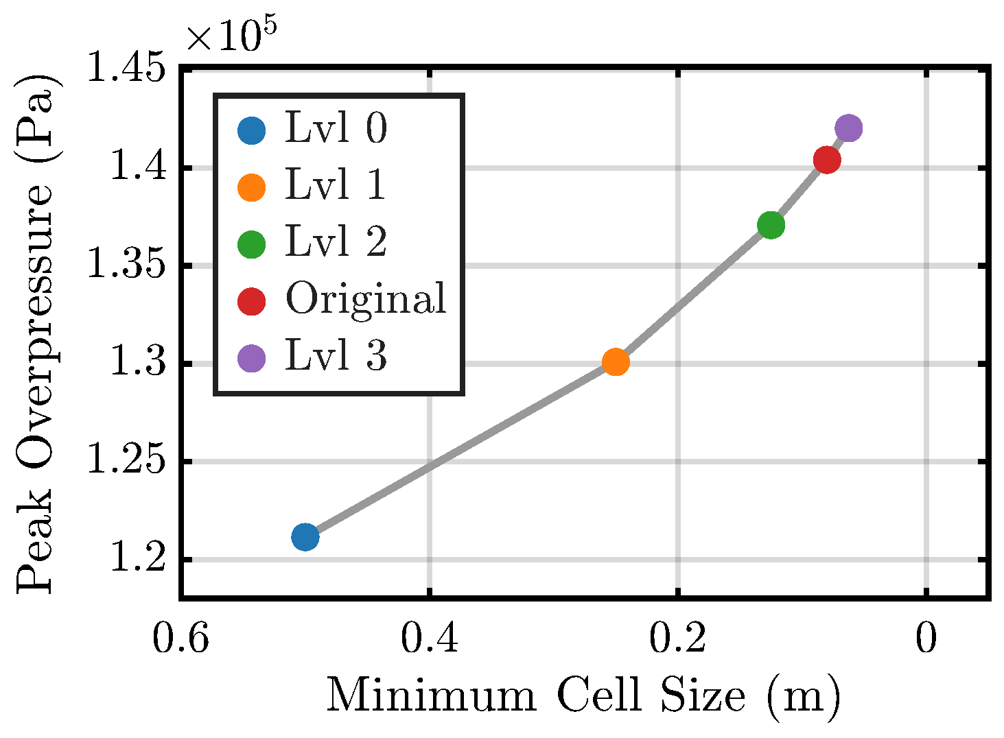
To validate the empirical models of Section 2.3, the high-explosive detonation library blastFoam [31] was used to simulate the evolution of overpressure and wind for a single instance of a blast pressure wave. This work modified the 2-dimensional Kingery–Bulmash axisymmetric wedge validation case provided with blastFoam to collect model validation data, which simulates a 10 kg spherical mass of TNT at the origin of the environment. To gather data for a wider range, the domain radius was extended from 16 m to 100 m, the mesh resolution from 25 cells along each axis (∼$0.64$ m per base cell) to 200 cells along the axis (∼$0.5$ m per base cell), and the simulation end time from 0.025 s to 0.1 s. OpenFOAM provides an adaptive mesh refinement (AMR) tool, adaptiveFvMesh, which refines the base mesh of an environment to a specified level [31]. A mesh refinement level of 3 was used to refine the base mesh to a minimum cell size of 0.0625 m, which is less than the 0.08 m minimum cell size in the default (blastFoam-provided) simulation. To verify mesh independence, the simulated peak overpressure was collected at a point 10 m from the origin over time for adaptive mesh refinement levels of 0–3 as shown in Figure 6. The peak overpressure at the same point in the original validation case is also shown for comparison, highlighting the model improvement that our finer base mesh provided to collect validation data for this work. The asymptotic convergence toward a stable, grid-independent limit verifies the spatial convergence of the numerical solution [32,33].

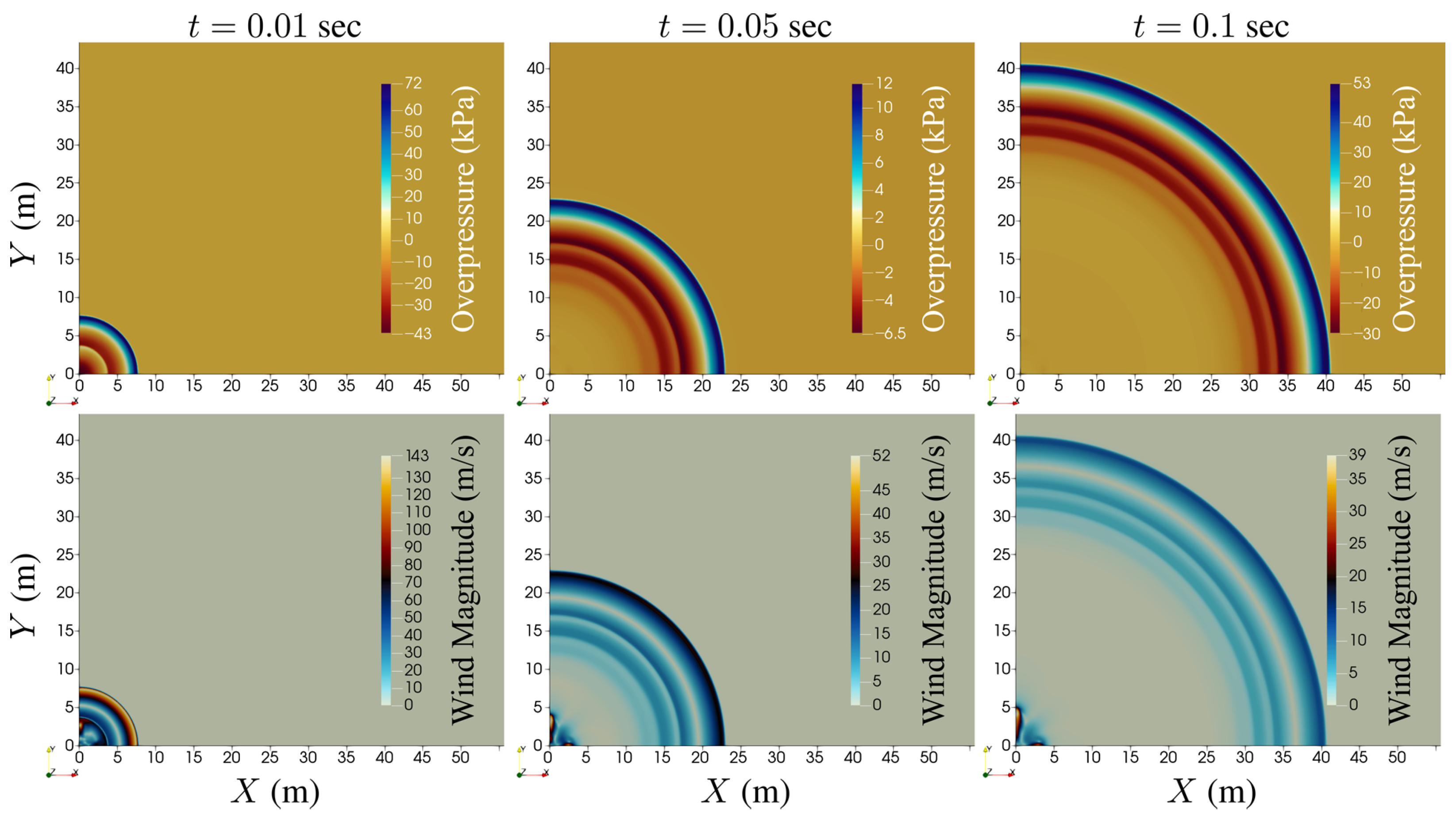
To collect the full set of validation data, overpressure and wind magnitude data were collected along a line extending 30 m radially from the origin, with a resolution of 0.001 m for every simulated time step, with standard linear interpolation for exported data between defined cells. The final level 3 AMR simulation required approximately 24 h of CPU time using 32 cores of an AMD Ryzen Threadripper 3990X 64-Core processor, 2.2 GHz CPU, and 256 GB of RAM. Resultant data for the radial evolution of overpressure and wind magnitude over time are shown in Figure 7.

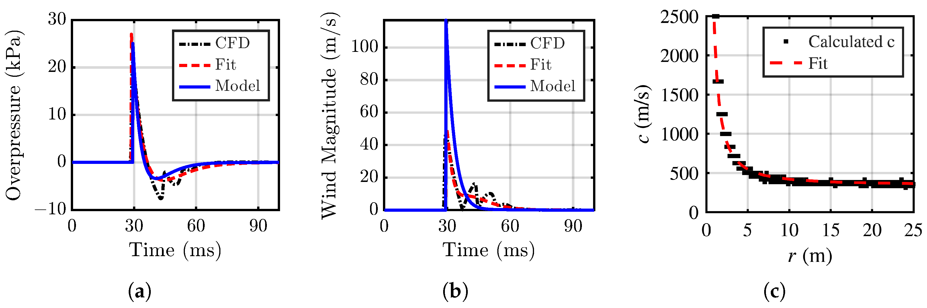
To compare the presented models to the simulated blast data, the parameters for the air velocity model (7) were chosen using Figure 1a, and the parameters for the Friedlander pressure wave models (5) were chosen using (2) and (3). An alternate set of parameters for the models (5) and (7) was also fit to the data using nonlinear least-squares data-fitting with the MATLAB lsqcurvefit function [34]. Figure 8a,b compares the model, fitted, and CFD data for one radial distance from the blast origin. Additionally, the propagation velocity c was calculated by comparing the propagation of the peak overpressure over a length scale of ∼0.5 m in the simulation over time, which is roughly the wheelbase of a large quadrotor UAV. The propagation velocity was calculated for the entire region of data collection as shown by the black dots in Figure 8c, which were used to create a two-term power series model of the form

$$c\left(\overline{x}\right)=1943·{\overline{x}}^{-1.397}+343,$$

(27)

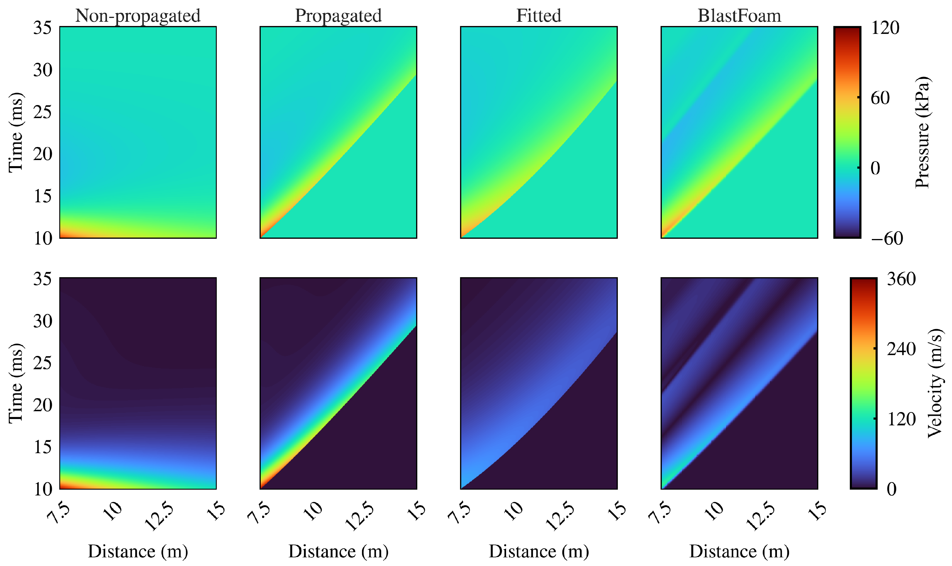
using the MATLAB fit function [35]. The model converges to a value of ∼343 (m/s) over the 30 m region of interest within the $0.1$ s simulation, which is comparable to prior work [6,36]. The peak amplitudes of the pressure from CFD and the model (5) with empirical parameters are very similar in Figure 8a. However, the positive phase duration parameter $\tau$ predicted by the empirical model is about half of the duration shown for the CFD-simulated pressure. The most significant difference between the proposed models and the CFD data is the difference in the peak wind magnitude values, which can be attributed to the Dewey model being originally developed to represent much larger explosions than the ones being simulated here. The results confirm that the pressure and velocity models can be obtained with empirically chosen parameters and be tuned to match CFD simulations. One notable difference is the presence of aftershocks that are not present in the empirical model. The aftershocks appear as follow-on oscillations in velocity that are visible as alternating bands of dark/light blue in the right panel of Figure 9 and as rings in Figure 7.

Figure 9 provides another illustration of the convected wave assumption. Column 1 corresponds to the pressure and velocity models from Section 2.1, highlighting that without the propagation speed, the models can only predict the pressure and velocity at a single given location over time. The non-propagated models show that the quantities decrease as expected as the distance from the blast increases, but because the models do not account for the propagation of the wave, the models only decay with time. Column 2 highlights the effects of utilizing the propagation speed defined by (27) in the models defined in Section 2.3. The parameters for the pressure and velocity models were also chosen based on the models defined in Section 2.1 (e.g., $P_s\left(d\right),\tau \left(d\right)$ for pressure and $V_s,\alpha ,\beta ,a$ for velocity). Column 3 shows a best fit for a grid of times and distances, extending the single distance case shown in Figure 8. Figure 9 highlights the differences between the proposed models and the CFD data more clearly by showing the spatiotemporal difference between the peak velocity predicted by (7) and that predicted by the CFD. The maximum error between the proposed pressure model and the CFD data was ∼$70.63$ kPa, with a root-mean-squared error (RMSE) of ∼$4.22$ kPa for the entire region of interest. Similarly, the maximum error between the proposed velocity model and the CFD data was ∼$137.5$ m/s, with an RMSE of ∼$9.46$ m/s for the entire region of interest.

4.2. Flight Simulation Testing

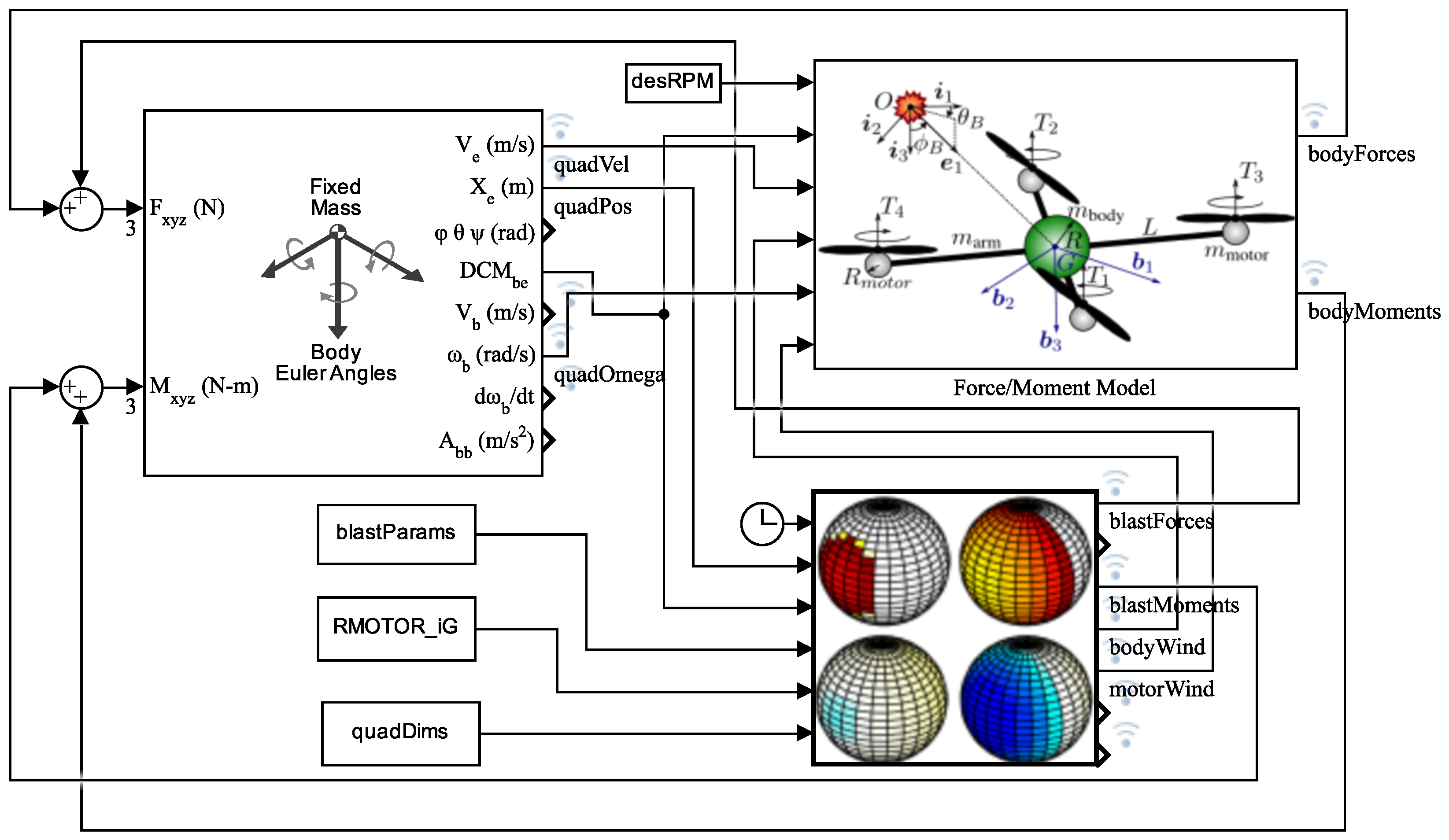
The Simulink model shown in Figure 10 was developed to evaluate the dynamic response of a quadrotor to a nearby explosion [15]. At each simulation time step, the blast and drag forces for each individual sphere in the multi-element quadrotor are computed. Due to the spatiotemporal disturbance model, each sphere experiences different pressure and drag loads. The net forces and moments are continuously recalculated based on the evolving blast pressure wave and the quadrotor’s evolving position in the disturbance field. Since the duration of the modeled overpressure data shown in Figure 8a is ∼30 ms, and the modeled particle velocity data shown in Figure 8b is ∼60 ms, all presented results are simulated for 90 ms. To ascertain the response of the vehicle during the blast event, a constant hover thrust is used for the duration of the simulations (i.e., assuming the quadrotor does not actively react to reject the disturbance over such a short time scale). Choosing different values for hover thrust during this simulation period to analyze the sensitivity of the vehicle to thrust changes would bias the terminal states in the respective direction that the thrust was varied, as there is no controller implemented, and the mass of the vehicle components is held constant to facilitate this analysis.

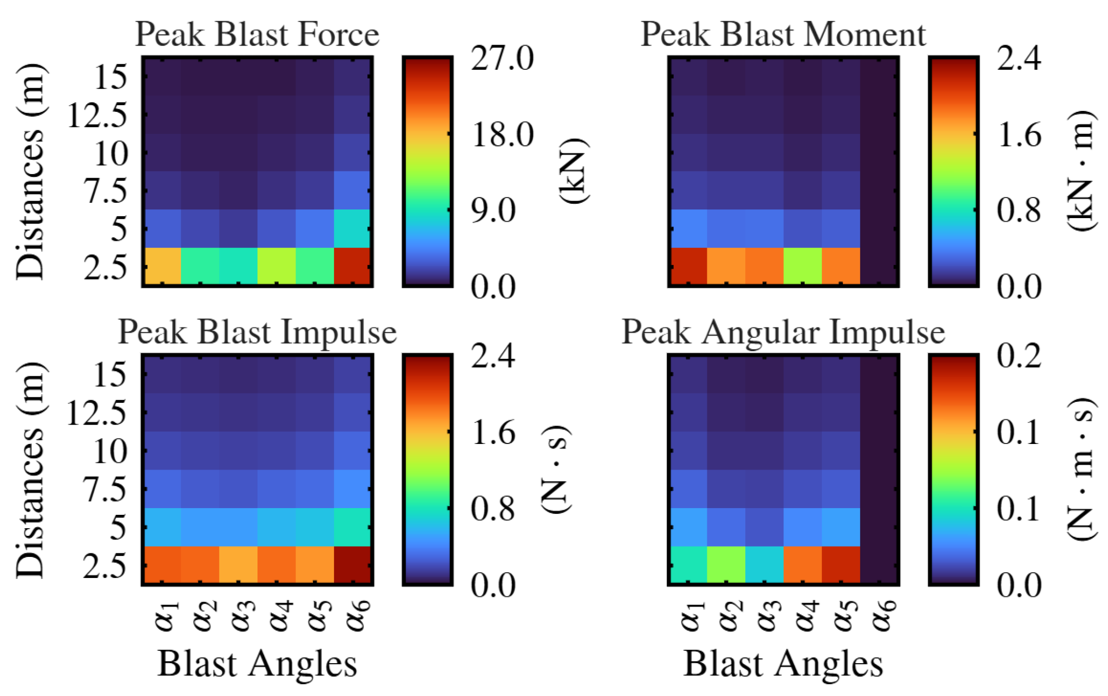
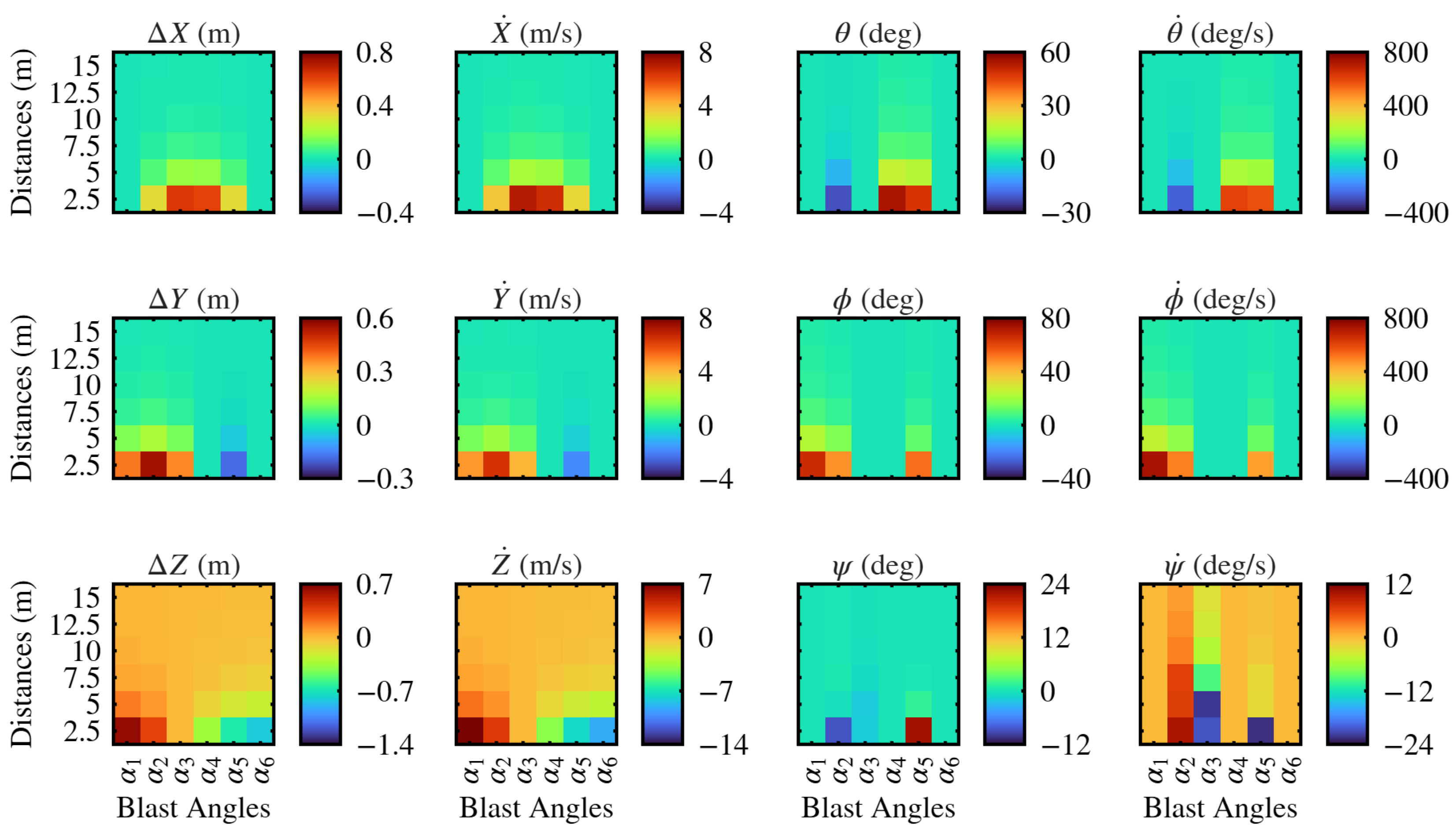
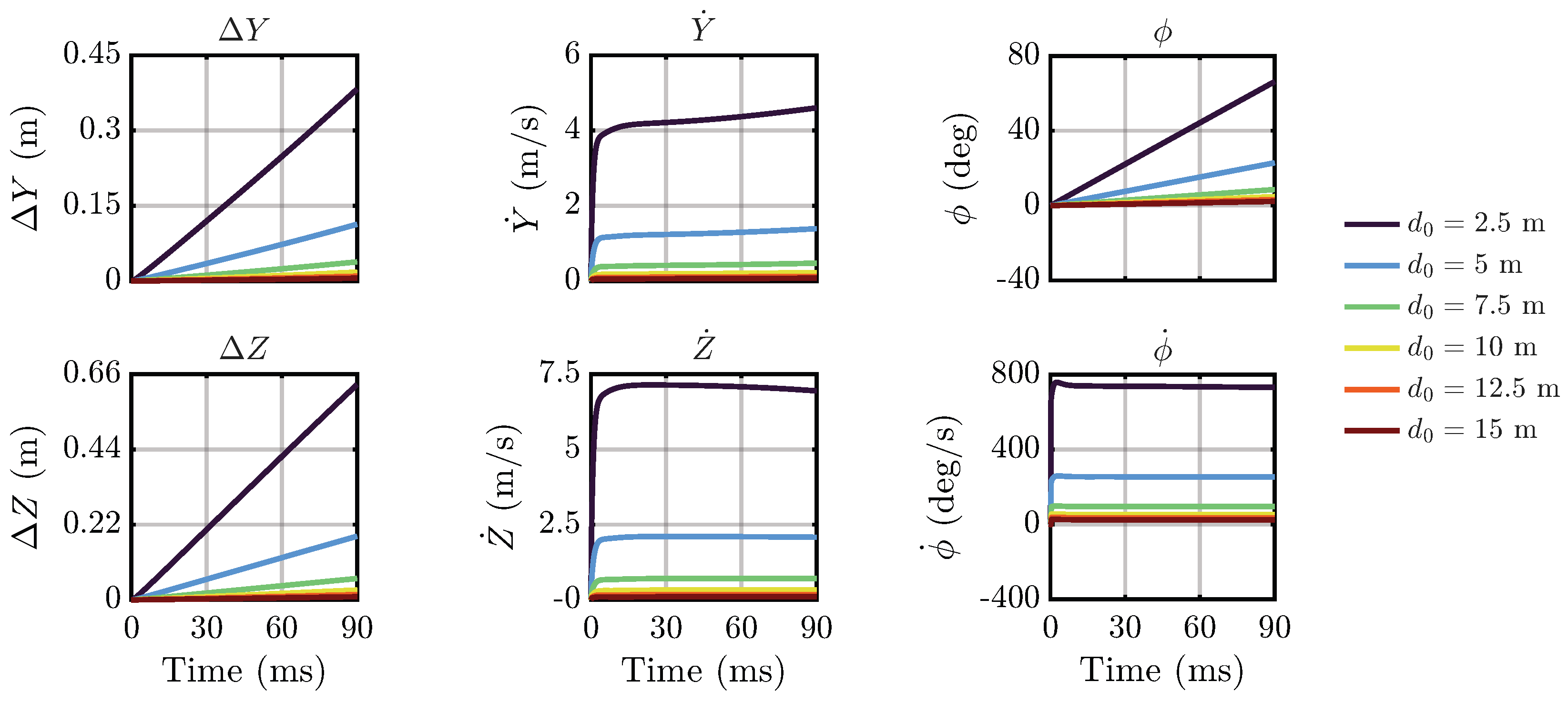
A range of $d_0\in \left\{2.5,5,7.5,10,12.5,15\right\}$ m values are used to initialize the position of the vehicle at a set standoff distance from the blast, with all other states initialized at zero. A series of blast angles ${\alpha }_i=({\theta }_{B,i},{\varphi }_{B,i})$ are simulated for each $d_0$, where the explosion makes contact with the vehicle at angles ${\theta }_B=(90-30(i-1))°$ and ${\varphi }_{B,i}=(150-30(i-1))°$, where $i\in \mathbb{Z}|1\le i\le 6$, according to Figure 5. Other properties used for the simulation are explosive mass $W=10$ kg, $R=R_{\mathrm{motor}}=0.05$ m for the motor and body spheres, $C_D=0.47$ for the drag coefficient, $L=0.15$ m for arm length, and $m_{\mathrm{motor}}=0.2$ kg, $m_{\mathrm{body}}=1$ kg, and $m_{\mathrm{arm}}=0.05$ kg for the mass of each constituent part. Figure 11 shows the terminal states of the quadrotor for each simulated case, while Figure 12 shows the corresponding peak force, moment and impulse values. The time series plots for all $d_0$ values at ${\alpha }_1=(90°,150°)$ are shown in Figure 13. The parameters vary as expected for each case, with nearer explosions leading to more significant perturbations. The simulation’s runtime statistics for 200 runs are shown in

Table 2. Summary of runtime statistics (200 runs).

Statistic	Time
Mean	1.10 s
Median	1.08 s
Standard deviation	97.3 ms
Minimum	1.03 s
Maximum	2.26 s

for simulations with an end time of 90 ms and a timestep of 0.1 ms for a total of 900 simulation time steps.

To calculate these statistics, the wall-clock time was collected per simulation using the timer function in MATLAB. The initial run takes the longest as Simulink requires time to load the model into memory for the first simulation, requiring up to 30 s in some cases to initialize and run the simulation. The overall runtime for each simulation after the model is initialized is ∼$1.1$ s. Based on the total simulation time steps, each time step took ∼$1.22$ ms to process, giving an extensible time estimate for any given set of simulation time parameters.

4.3. Sensitivity Study

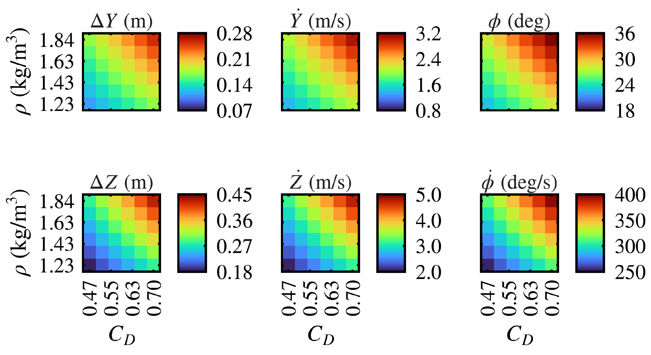
This work utilizes simple constant drag coefficient and constant air density assumptions, recognizing that more accurate models can be integrated in future work (see Section 5). However, to provide some insight into the degree to which these parameters affect the predicted terminal state of the UAV, a sensitivity analysis was performed. The sensitivity analysis parametrically varied the drag coefficient from $C_D=0.47$ and $\rho =1.225$ kg/m³ to 1.5 times their nominal values, assuming both air density and the drag coefficient of a sphere would increase based on the blast conditions considered here. The results in Figure 14 illustrate the terminal states for a single case of ${\alpha }_1=(90°,150°)$ at a fixed standoff distance of $d_0=5\mathrm{m}$. The results illustrate that the terminal states scaled linearly with $C_D$ and $\rho$.

5. Discussion of Modeling Limitations

While the model established in this paper can be useful for identifying trends in the response of the quadrotor to different distances, explosive mass, or blast angles, there are several limitations that can potentially be improved in future work and are briefly discussed below.

5.1. Limitations Due to Quadrotor Geometry and Shock-Wave Interactions Modeling

One can expect that significant blast-induced forces and moments are experienced by a small UAV for a brief period of time on the order of about 1 to 10 ms, depending on blast parameters and standoff distance. The interaction of the blast with the UAV can be decomposed into two phases: (1) the initial phase of reflection/diffraction of the blast wave as it rapidly passes over the UAV, and (2) a second phase that begins once the initial wavefront has passed and ends when the conditions have returned to near ambient. During the first phase, as the blast wave progresses over the vehicle’s body, one expects that each individual component (e.g., motor, propeller) will experience its own reflected shock on the side facing the blast wave, followed by diffractive waves that wrap around each component as the wavefront continues to engulf the vehicle. Individual shocks may interact and merge, depending on their geometry. The approach proposed in this paper captures only the diffractive loads under the convected wave assumptions (as described in Section 2, it does not model shock wave formation or additional overpressure due to reflection). The relations (6) and (8) ignore the physical presence of the UAV itself and how it may alter and interact with the flow. Moreover, the quadrotor is modeled as a set of spheres; the diffractive loads over a more complex geometry would differ.

5.2. Limitations of the Thrust Model

Blast waves can have a significant effect on thrust production, potentially through mechanisms such as shock formation, blast-induced wind, and bending and vibration of propeller blades. Modeling thrust variation during the initial phase of the blast is particularly difficult and requires computational fluid dynamics (CFD) coupled with finite element analysis (FEA) to capture the aero-elastic response of propellers and components. However, during this first phase, diffractive loads can be expected to dominate. In the second phase, once the wavefront has passed over the vehicle, the resulting blast-induced wind can continue to affect thrust production. Once subject to the blast-induced wind, propellers may be operating in either a subsonic, transonic, or supersonic flow depending on blast parameters. To our knowledge, there is no existing literature characterizing small UAV propeller thrust forces at these high flow speeds. The model in this work assumes a constant hover thrust. For low subsonic flows, there exist three common operating conditions for the propellers on a multirotor: (1) air flow directed into the propellers during climbs or aggressive forward flight, (2) direct or reverse non-axial inflow caused by steady forward flight or cruising, and (3) reverse inflow directed into the prop-wash of the propellers during descent or rapid decelerations [37,38]. The thrust load variation caused by typical operating conditions (i.e., at low speeds) of a multirotor depends on several critical flow regimes identified as windmill brake state, turbulent wake state, and vortex ring state (we refer the reader to [37,38,39]). In general, these states can lead to a reduction in thrust and unsteadiness in thrust production.

5.3. Limitations of the Aerodynamic Model

The limitations of the aerodynamic model in this paper include those mentioned previously: shock-wave interactions are not modeled and air density and drag coefficient are assumed constant. Analytical models that capture density changes across a shock (for example, the Rankine–Hugoniot relation [10] alongside isentropic flow relations behind the shock) could potentially provide an improved approximation; however, detailed shock-wave interaction with the quadrotor geometry requires CFD analysis. Furthermore, it is well known that the drag coefficient of a sphere varies dramatically in compressible flows due to shock-boundary layer interactions and wave drag. Depending on the flow regime, various models of $C_D$ as a function of Mach number M and Reynolds number $Re$ are available  [40,41,42] and could potentially be integrated in future work. The use of a constant drag coefficient in this work (and the fitted Mach range of the Dewey model) limits the applicability of this work to flows with peak velocities $<1$ Mach—a region which is based on explosive mass and standoff distance.

5.4. Damage Modeling and Survivability

The model proposed in this paper assumes that the UAV suffers no damage, regardless of proximity to the blast. The simulation could be further improved by modeling the damage assessment due to blasts on the entire aircraft, similar to [14], or to individual components such as propellers [43,44]. A major extension to the survivability analysis of a quadrotor to nearby blast disturbances would be a more extensive test suite of the experiments conducted in [11] to evaluate a range of blast characteristics that lead to catastrophic UAV failure.

6. Conclusions

This work presented a dynamic model of a quadrotor that includes the effects of blast-induced overpressure (diffractive loads) and blast-induced wind (drag) parametrized by empirical models that extended prior work (for a single point in space) into a spatiotemporal disturbance field assuming plane wave propagation around the vicinity of the quadrotor. The quadrotor motors and body were represented as a rigid body consisting of connected spheres to facilitate computation. Simulations for varying standoff distances predicted the state of the quadrotor 90 ms after the blast.

By determining the terminal state immediately after the blast, the simulation tool supports control design. The terminal state can be used as an initial condition to evaluate controllers that aim to provide robustness and recovery to blast disturbances. Future work may include validating the model through experiments or further CFD simulations, as well as refining the approach to address model limitations.

References

1. Irimia, A.; Găman, G.A.; Pupăzan, D.; Ilie, C.; Nicolescu, C. Using Drones in Support of Rescue Interventions Teams in Toxic/Flammable/Explosive Environments. Environ. Eng. Manag. J. 2019, 18, 831–837. [Google Scholar] [CrossRef]
2. Kim, K.; Davidson, J. Unmanned Aircraft Systems Used for Disaster Management. Transp. Res. Rec. 2015, 2532, 83–90. [Google Scholar] [CrossRef]
3. Bamford, T.; Medinac, F.; Esmaeili, K. Continuous Monitoring and Improvement of the Blasting Process in Open Pit Mines using Unmanned Aerial Vehicle Techniques. Remote Sens. 2020, 12, 2801. [Google Scholar] [CrossRef]
4. Louk, J.; Salzman, M.; Kim, M.; Melendez, A.; Manjunath, P.; Doscher, D.; Bluman, J.E. Overpressure Effects on Quadcopter Stability from Tank Muzzle Blasts. In Proceedings of the AIAA SciTech 2023 Forum and Exposition, National Harbor, Maryland, USA and Online, 23–27 January 2023; p. 1732. [Google Scholar] [CrossRef]
5. Bowen, I.G.; Albright, R.W.; Fletcher, E.R.; White, C.S. A Model Designed to Predict the Motion of Objects Translated by Classical Blast Waves; Technical Report; Lovelace Foundation for Medical Education and Research: Albuquerque, NM, USA, 1961. [Google Scholar] [CrossRef][Green Version]
6. Needham, C.E. Blast Waves; Springer: Cham, Switzerland, 2017; Volume 2. [Google Scholar] [CrossRef]
7. Friedlander, F.G. The Diffraction of Sound Pulses I. Diffraction by a Semi-Infinite Plane. Proc. R. Soc. Lond. Ser. A Math. Phys. Sci. 1946, 186, 322–344. [Google Scholar] [CrossRef] [PubMed]
8. Dewey, J. The Air Velocity in Blast Waves From TNT Explosions. Proc. R. Soc. Lond. Ser. A Math. Phys. Sci. 1964, 279, 366–385. [Google Scholar] [CrossRef]
9. Brode, H.L. Blast Wave from a Spherical Charge. Phys. Fluids 1959, 2, 217–229. [Google Scholar] [CrossRef]
10. Kandula, M.; Freeman, R. On the Propagation and Interaction of Spherical Blast Waves. In Proceedings of the 37th AIAA Fluid Dynamics Conference and Exhibit, Miami, FL, USA, 25–28 June 2007; pp. 2007–4117. [Google Scholar] [CrossRef][Green Version]
11. Martin, J.E.; Saul, V.; Novick, D.; Allen, D. Assessing the Vulnerability of Unmanned Aircraft Systems to Directed Acoustic Energy; Technical Report; Sandia National Lab: Albuquerque, NM, USA, 2020. [Google Scholar] [CrossRef] [PubMed]
12. Han, L.; Han, Q.; Ge, Y.X.; Sang, X.Q. Vulnerability Assessment of Combat Aircraft to Blast Loading. Proc. Inst. Mech. Eng. Part G J. Aerosp. Eng. 2019, 233, 604–615. [Google Scholar] [CrossRef]
13. Zhang, M.t.; Pei, Y.; Yao, X.; Ge, Y.x. Damage Assessment of Aircraft Wing Subjected to Blast Wave with Finite Element Method and Artificial Neural Network Tool. Def. Technol. 2023, 25, 203–219. [Google Scholar] [CrossRef]
14. Feng, X.; Yang, Z.; Nie, Y. Investigation of the Overall Damage Assessment Method Used for Unmanned Aerial Vehicles Subjected to Blast Waves. Aerospace 2024, 11, 651. [Google Scholar] [CrossRef]
15. Kakavitsas, N.P.; Willis, A.; Maity, D.; Wolek, A. A Quadrotor Model for Evaluating Dynamic Response to a Blast Pressure Wave. In Proceedings of the AIAA SciTech 2025 Forum and Exposition, Orlando, FL, USA, 6–10 January 2025. [Google Scholar] [CrossRef]
16. Chandra, N.; Ganpule, S.; Kleinschmit, N.; Feng, R.; Holmberg, A.; Sundaramurthy, A.; Selvan, V.; Alai, A. Evolution of Blast Wave Profiles in Simulated Air Blasts: Experiment and Computational Modeling. Shock Waves 2012, 22, 403–415. [Google Scholar] [CrossRef]
17. Goel, M.; Matsagar, V.; Gupta, A.; Marburg, S. An Abridged Review of Blast Wave Parameters. Def. Sci. J. 2012, 62, 300–306. [Google Scholar] [CrossRef]
18. Sadovskiy, M.A. Part 1: Mechanical and Seismic Effect of the Explosion. In Selected Works: Geophysics and the Physics of Explosion; Chapter Part 1: Mechanical Seismic Action and Explosion; Nauka: Moscow, Russia, 2004; pp. 7–49. [Google Scholar]
19. Jankura, R.; Zvaková, Z.; Boroš, M. Analysis of mathematical relations for calculation of explosion wave overpressure. In Proceedings of the CBU International Conference on Innovations in Science and Education, Prague, Czech Republic, 18–20 March 2020. [Google Scholar]
20. Lukić, S.; Draganić, H.; Gazić, G.; Radić, I. Statistical analysis of blast wave decay coefficient and maximum pressure based on experimental results. In Proceedings of the Structures Under Shock and Impact XVI; WIT Press: Southampton, UK, 2020; Volume 198, pp. 65–76. [Google Scholar] [CrossRef]
21. Bajić, Z.; Bogdanov, J.; Jeremić, R. Blast effects evaluation using TNT equivalent. Sci. Tech. Rev. 2009, 59, 50–53. [Google Scholar]
22. Gelfand, B. Translation from Russian to English the Book “Blast Effects Caused by Explosions” Authored by B. Gelfand and M. Silnikov; Contract Number N62558-04-M-0004; Technical Report; United States Army, European Research Office of the U.S. Army: London, UK, 2004.
23. Gibson, P. Blast Overpressure and Survivability Calculations for Various Sizes of Explosive Charges; Technical Report ADA286212; U.S. Army Natick Research, Development and Engineering Center: Natick, MA, USA, 1994.
24. Remennikov, A.M. A Review of Methods for Predicting Bomb Blast Effects on Buildings. J. Battlef. Technol. 2003, 6, 5–10. [Google Scholar]
25. Kingery, C.N.; Bulmash, G. Airblast Parameters From TNT Spherical Air Burst and Hemispherical Surface Burst; Technical Report ARBRL-TR-02555; U.S. Army Ballistic Research Laboratory: Aberdeen Proving Ground, MD, USA, 1984.
26. Paris, L.; Dubois, A. Recent Developments to Evaluate Global Explosion Loading on Complex Systems. J. Loss Prev. Process Ind. 2017, 46, 163–176. [Google Scholar] [CrossRef]
27. Ritzel, D.V.; Van Albert, S.; Sajja, V.; Long, J. Acceleration from Short-Duration Blast. Shock Waves 2018, 28, 101–114. [Google Scholar] [CrossRef]
28. Rohatgi, A. WebPlotDigitizer, Version 4.7. Available online: https://automeris.io/ (accessed on 10 June 2026).
29. The MathWorks, Inc. MATLAB Optimization Toolbox: fmincon-Find Minimum of Constrained Nonlinear Multivariable Function, Natick, MA, USA, 2024. MATLAB Optimization Toolbox Function, Release R2024a. Available online: https://www.mathworks.com/help/optim/ug/fmincon.html (accessed on 10 July 2026).
30. Hoerner, S.F. Fluid-Dynamic Drag: Practical Information on Aerodynamic Drag and Hydrodynamic Resistance; Hoerner Fluid Dynamics: Bakersfield, CA, USA, 1965. [Google Scholar]
31. Heylmun, J.; Vonk, P.; Brewer, T. blastFoam, version 6.0; Synthetik Applied Technologies: Austin, TX, USA, 2022; Available online: https://www.blastfoam.org/ (accessed on 10 July 2026).
32. Roache, P.J. Verification and Validation in Computational Science and Engineering; Hermosa Publishers: Albuquerque, NM, USA, 1998. [Google Scholar]
33. Toro, E.F. Riemann Solvers and Numerical Methods for Fluid Dynamics: A Practical Introduction, 3rd ed.; Springer Science & Business Media: Berlin/Heidelberg, Germany, 2013. [Google Scholar]
34. The MathWorks, Inc. MATLAB Optimization Toolbox: lsqcurvefit-Solve Nonlinear Curve-Fitting (Data-Fitting) Problems in Least-Squares Sense) Problems in Least-Squares Sense, Natick, MA, USA, 2026. MATLAB Optimization Toolbox Function, Release R2026a. Available online: https://www.mathworks.com/help/optim/ug/lsqcurvefit.html (accessed on 10 July 2026).
35. The MathWorks, Inc. MATLAB Curve Fitting Toolbox: fit-Fit Curve or Surface to Data, Natick, MA, USA, 2026. MATLAB Curve Fitting Toolbox Function, Release R2026a. Available online: https://www.mathworks.com/help/curvefit/fit.html (accessed on 10 July 2026).
36. Rigby, S. Blast Wave Time of Arrival: A Reliable Metric to Determine Pressure and Yield of High Explosive Detonations; Technical Report 79; The University of Sheffield: Sheffield, UK, 2021. [Google Scholar]
37. Cerny, M.; Breitsamter, C. Investigation of Small-scale Propellers Under Non-axial Inflow Conditions. Aerosp. Sci. Technol. 2020, 106, 106048. [Google Scholar] [CrossRef]
38. Liu, C.; Wang, Y.; Wei, Z. Effects of Vectorial Inflow on the Multi-Axis Aerodynamic Performance of a Small-Sized UAV Rotor. Aerospace 2025, 12, 1096. [Google Scholar] [CrossRef]
39. Veismann, M.; Dougherty, C.; Gharib, M. Effects of Rotor Separation on the Axial Descent Performance of Dual-Rotor Configurations. Flow 2023, 3, E7. [Google Scholar] [CrossRef]
40. Loth, E.; Daspit, J.T.; Jeong, M.; Nagata, T.; Nonomura, T. Supersonic and Hypersonic Drag Coefficients for a Sphere. AIAA J. 2021, 59, 3261–3274. [Google Scholar] [CrossRef]
41. Singh, N.; Kroells, M.; Li, C.; Ching, E.; Ihme, M.; Hogan, C.J.; Schwartzentruber, T.E. General Drag Coefficient for Flow over Spherical Particles. AIAA J. 2021, 60, 2. [Google Scholar] [CrossRef]
42. Morrison, F.A. An Introduction to Fluid Mechanics; Cambridge University Press: Cambridge, UK, 2013. [Google Scholar]
43. Jiang, Z.; Ma, R.; Lu, F.; Zhu, H.; Lan, Y.; Xue, X.; Zhang, S.; Wu, C. Damage Identification of Multirotor UAV Propellers via Unsteady Coupling Association. Measurement 2024, 243, 116364. [Google Scholar] [CrossRef]
44. Lee, G.; Park, S.; Choi, S.; Lee, S.; Jeong, J.; Lee, D. Classification and Diagnosis of Propeller Damages Using FFT-Based Motor Current Signature Analysis of DC-Link Current. IEEE Access 2026, 14, 35126–35139. [Google Scholar] [CrossRef]
Figure 1. (a) Parametric curves fitted to blast model parameter data from [8]. (b) Wind Mach number over time at a point in space 7.5 m from a 10 kg explosive, giving a scaled distance of S = 3.48 m/kg1/3 which is within the original data range provided in [8].
Aerospace 13 00646 g001
Figure 2. (a) Overpressure over time of a Friedlander pressure wave for a stationary point in space. (b) Corresponding axial force for a sphere of radius R = 0.15 m. (c) Time-evolution of pressure over the surface of a sphere.
Aerospace 13 00646 g002
Figure 3. (a) Planar wave assumption, (b) spherical spreading assumption, (c) max percent difference in peak blast force over a range of R / d 0 ratios for a sphere of R = 0.25 m.
Aerospace 13 00646 g003
Figure 4. Models (dark lines) fitted to the experimental results (light-colored lines) from a digitized version of Figure 5 from [27] with fitted parameters shown in Table 1.
Aerospace 13 00646 g004
Figure 5. Multi-link model of a quadrotor with a nearby explosion.
Aerospace 13 00646 g005
Figure 6. The peak overpressure and minimum mesh size of the original validation case are shown in red, while the same data for the updated domain simulations presented in this work are shown in other representative colors, all asymptotically converging toward a stable limit.
Aerospace 13 00646 g006
Figure 7. Evolution of top: overpressure and bottom: air velocity magnitude for three simulated time steps. The range of colorbar values is clamped to the range of values for that respective time step.
Aerospace 13 00646 g007
Figure 8. Comparison of (a) overpressure, and (b) wind magnitude at a distance of 15 m from the blast. (c) Fitted propagation speed over the entire domain for a 0.5 m length scale, representative of a large quadrotor UAV.
Aerospace 13 00646 g008
Figure 9. Column 1 and 2: non-propagated/propagated empirical models, Column 3: Best fit model minimizing the difference between the model and the CFD data, Column 4: CFD data.
Aerospace 13 00646 g009
Figure 10. Simulink model used for blast response simulation.
Aerospace 13 00646 g010
Figure 11. Terminal UAV states at various standoff distances and blast angles after 90 ms.
Aerospace 13 00646 g011
Figure 12. Peak simulated blast forces, moments, and their respective impulses for each tested standoff distance and blast angle after 90 ms.
Aerospace 13 00646 g012
Figure 13. Transient UAV states over 90 ms for all tested standoff distances and α 1 . At short standoff distances, the blast perturbs the attitude such that the constant thrust pulls the quadrotor along the inertial + Y direction, causing the upwards trend for Y ˙ .
Aerospace 13 00646 g013
Figure 14. Parametric sensitivity study of the variation of terminal states based on a range of constant drag coefficients and a range of constant air densities α 1 = ( 90 ° , 150 ° ) at a fixed standoff distance of d 0 = 5 m .
Aerospace 13 00646 g014