Modal Parameter Identification of the New Type of Airship with Multi-Airbag Hybrid Configuration Based on the Stochastic Subspace Method

Abstract

The new type of multi-airbag hybrid airship is a novel lighter-than-air platform, but its flexible structures pose challenges for accurate modal parameter identification under complex fluid-structure interaction. Traditional methods often fail to capture the dynamic characteristics of such compliant systems. In this paper, a stochastic subspace identification method is proposed to estimate the modal parameters of the three capsule hybrid airship. The method constructs the Hankel matrix using only output response data and extracts the system matrix by singular value decomposition so as to identify the natural frequency and damping coefficient. Moreover, the numerical model of the airship (aspect ratio 2.22) is built, and the simulated response data (first five modes) are used to validate the approach. The results show that the identified frequencies and damping ratios match the theoretical values with a maximum error of 6.35%, demonstrating good accuracy and robustness. The proposed technique can provide a reliable tool for online modal identification of flexible airships, supporting structural health monitoring and vibration control.

1. Introduction

With the continuous development of aerospace technology, airships, as a kind of lighter-than-air vehicle with unique advantages, show a wide range of application prospects in the fields of military reconnaissance, logistics and transportation, and aerial monitoring [1,2]. As a new type of airship structure, the multi-airbag hybrid layout airship combines the advantages of traditional airships and multibody airships with a smaller size and simpler structure, which can better meet the diversified demands of modern aerospace missions on the performance of airships [3]. However, airships are subject to a variety of complex loads during flight, and the dynamic response characteristics of their structures are directly related to flight safety and mission execution results [4,5]. Modal parameters, as the key indexes describing the dynamic characteristics of the structure, are of vital significance for the optimized design, vibration control, and health monitoring of airship structures [6,7,8].

Traditional modal parameter identification methods are mostly developed for rigid structures. For flexible airbag airships with complex nonlinear characteristics, however, these methods often fail to ensure sufficient accuracy and reliability [9,10,11]. As an advanced modal parameter identification method, the stochastic subspace method can effectively handle the structural dynamic response problem under random excitation, which provides a new way to accurately identify the modal parameters of airships [12,13]. Wang et al. [14] used the stochastic subspace method to identify the modal parameters of the modified data for the modal parameter test of engineering structures and achieved the asynchronous measurement of bridge modes; P.-É. Charbonnel [15] evaluated the robustness of the modal analysis and identification method based on stochastic subspace and supported the numerical research through the experimental structure. Gustavo Wagner [16] used the stochastic subspace identification (SSI) method to realize the modal identification of light flexible wind turbine blades under wind excitation and achieved good identification results in the target frequency band.

Therefore, this paper proposes an identification method for structural modal parameters. This method is designed for in-flight identification of a multi-airbag hybrid configuration airship based on the stochastic subspace algorithm. Through theoretical derivation and simulation analysis, the dynamic characteristics of airship structure are deeply studied to solve the problem that the dynamic change of structure cannot be tested and simulated on the ground and provide a certain theoretical basis and technical support for the engineering application of airships.

2. Modeling a Multi-Airbag Hybrid Configuration Airship

The dimensions of the main bladder airship derived from the NACA4418 airfoil profile [17] for the design are shown in

Table 1. Main bladder airship size parameters.

Length (mm)	Width (mm)	Height (mm)
100	12.76 × 2 = 25.52	18.32

.

It should be noted that the dimensions presented in Table 1 correspond to a scaled laboratory model rather than a full-scale airship. The geometric scaling ratio is approximately 1:200 relative to a typical full-scale hybrid airship (for example, the Airlander 10, which has a length of approximately 92 m [18]). Such scaled models are widely employed in the preliminary design and validation phases of airship research, as they enable cost-effective experimental and numerical investigations while maintaining geometric similarity with the full-scale prototype.

Through the research on the data of the current in-service airships and literature references, it can be seen that the spindle-shaped airship with an aspect ratio of 3–5 can achieve the best solution for the aerostatic lift [12], aerodynamic, and structural design requirements. The current design has an aspect ratio of 4, which basically meets the requirements.

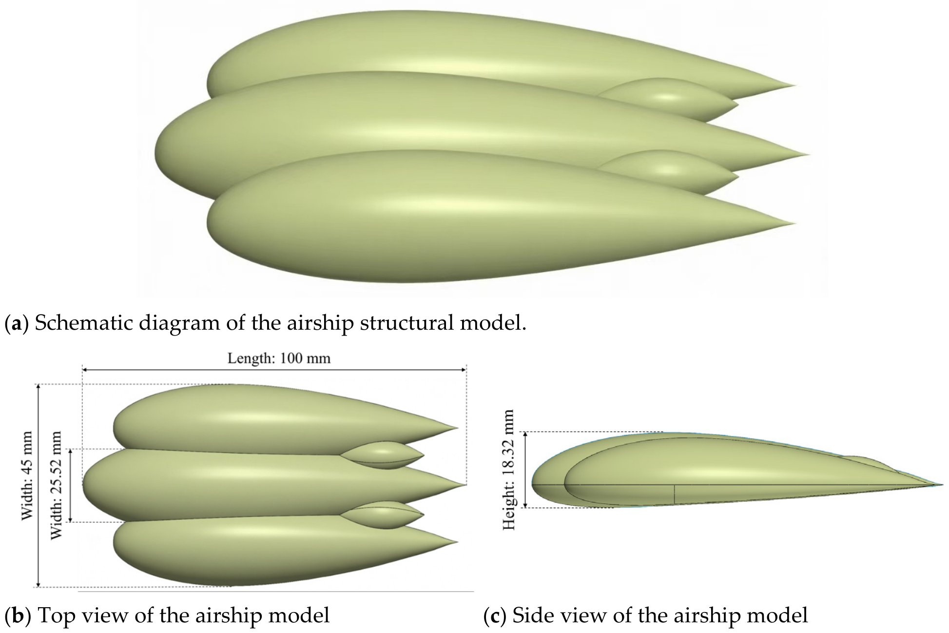
However, the resulting airship structure cannot fully leverage the compactness advantage of hybrid design, and the increase in size is limited. This makes it difficult to fully exploit the advantages of hybrid airships, which are inherently smaller and structurally simpler. As the object of this paper is a hybrid airship, which is a combination of three bladders, the required aspect ratio is smaller. Based on the Airlander 10 (aspect ratio ≈ 2.09 [18,19]), the target aspect ratio is set to 2.22. Starting from the main bladder dimensions (Table 1), two side bladders are added and adjusted in their lateral positions so that the total width of the assembly becomes 45 mm. This yields the final aspect ratio of 100/45 = 2.22. The geometric model is shown in Figure 1, where the overall width and height are indicated.

3. Constructing Recognition Models and Solving

3.1. Theoretical Modeling of the Stochastic Subspace Method

To identify the modal parameters of the hybrid airship structure, a Hankel matrix is first constructed following the SSI framework [20,21,22]. Singular value decomposition (SVD) and covariance matrix calculation are then performed on this Hankel matrix to extract the overall system matrices B and C, which contain the dynamic response and modal information. Subsequently, based on the relationship between modal parameters and the structural model, a modal analysis of the airship structure is conducted. Finally, the modal parameters are obtained through a modal synthesis analysis [23,24,25].

In the time-domain SSI method, let “p” denote the number of block rows in the Hankel matrix (which determines the order of the observability matrix), “q” is the number of block columns (which determines the order of the controllability matrix), and “n” is the system order, with p ≥ q ≥ n. The corresponding Hankel matrix of the airship structure can be decomposed into the product of the observability matrix and the controllability matrix:

$$H_{pq}=\left(\begin{array}{llll}{R}_1& R_2& \cdots & R_q\\ R_2& R_3& \cdots & R_{q+1}\\ ⋮& ⋮& ⋮& ⋮\\ R_p& R_{p+1}& \cdots & R_{p+q}\end{array}\right)=O_p{C}_q$$

(1)

where O_p is the p-th order observability matrix and C_q is the q-th order controllability matrix. These two matrices are further expressed as follows:

$$O_p=\left(\begin{array}{l}C\\ CB\\ ⋮\\ {C(B)}^{P-1}\end{array}\right)$$

(2)

$$C_q=(\mathrm{G} B\mathrm{G} \dots {(B)}^{q-1}\mathrm{G})$$

(3)

According to the standard SSI procedure, to obtain the matrices in Equations (2) and (3), singular value decomposition is applied to the Hankel matrix:

$$H_{pq}= US{V}^T=(R_1 R_2 )\left(\begin{array}{ll}{S}_1& 0\\ 0& S_2\end{array}\right)\left(\begin{array}{l}{V}_1^T\\ V_2^T\end{array}\right)$$

(4)

In the above SVD, U and V are orthogonal matrices; S is a diagonal matrix consisting of singular values. Specifically, R₁ is the diagonal matrix of the system’s non-zero singular values (arranged in descending order), R₂ is the diagonal matrix of noise-related singular values; U₁ and V₁ are the corresponding left and right singular vector matrices for S₁; U₂ and V₂ are those for S₂.

When the hybrid airship structure is subjected to stationary random load excitation, the noise singular value matrix S₂ Equation (4) can thus be simplified as follows:

$$H_{pq}= US{V}^T=R_1{S}_1 V_1^T$$

(5)

From a direct comparison of Equation (5) with the Hankel decomposition in Equation (1), the following is obtained:

$$\begin{array}{l}{O}_p=R_1{S}_1^{1/2}\\ C_q=S_1^{1/2} V_1^T\end{array}$$

(6)

Once the observability matrix O_p and controllability matrix C_q are obtained, the system matrices B and C of the airship structure can be further solved. Based on the shift-invariance property of the observability matrix, the following is obtained:

$$\begin{array}{l}C=E{O}_P\\ B={(C)}^{†}FO\end{array}$$

(7)

For the resulting airship structure, the middle matrix in matrices B and C is $E=(I_p,0_p,\dots 0_p)$ and the matrix is $F=(0_p,I_p,\dots 0_p)$. The output matrix C is extracted from the first block row of the observability matrix, and the least-squares solution via pseudoinverse is the appropriate mathematical treatment for overdetermined systems. This correction brings our derivation into alignment with standard subspace identification theory.

As a result, based on the airship structural system matrices B and C obtained by the system parameter identification method of the stochastic subspace method, the modal parameters of the structure can be further obtained by performing a modal analysis of the structural body based on the physical relationship between the modal parameters in the dynamic response model of the structure and the structural system model of the airship. The eigenvalue decomposition of the airship structural system matrix B can obtain the modal parameters:

$$B=\psi \mathsf{\Lambda }{\left(\psi \right)}^{-1}$$

(8)

where the matrix $\mathsf{\Lambda }$ is the eigenvalue of the discrete system of the overall structure of the airship $\mathsf{\Lambda }=diag({\lambda }_i), i=1,2,3\dots ,n$, ${\lambda }_i$ are eigenvalues of the overall structure of the airship, and $\psi \in C^{n\times n}$ is the matrix of eigenvectors of the structural system of the airship. The relationship between the eigenvalues of the airship system matrix B and the eigenvalues of the structural vibration ${({\lambda }_i)}^c$ can be expressed as follows:

$${({\lambda }_i)}^c={\displaystyle \frac{1}{\mathsf{\Delta }t}}\ln {\lambda }_i$$

(9)

In this expression, $\mathsf{\Delta }t$ is the value of the sampling time interval of the airship structural system; then, the intrinsic frequency and modal damping of the overall structural system of the airship can be calculated separately:

$${({\lambda }_i)}^c, {\overline{ ({\lambda }_i)}}^c=-{\xi }_i{\omega }_i^T\pm j{\omega }_i\sqrt{1-{({\xi }_i)}^2}$$

(10)

In this equation, j is an imaginary unit, and the eigenvalues ${({\lambda }_i)}^c$, ${\overline{ ({\lambda }_i)}}^c$ are conjugate transpositions of each other. Then, the vibration pattern of the overall structural system of the airship can be obtained by solving accordingly:

$$\phi =C\psi$$

(11)

The response data-driven stochastic state subspace-based method uses measured input–output stochastic response data to build a generalized Hankel matrix, which can be obtained by QR decomposition and SVD techniques, still using the state space equations of the linear dynamical system as the mathematical model:

$$\dot{x}(t)=A_{c}x(t)+B_{c}u(t)$$

(12)

where A_c is the state matrix of the continuous time state space equation of the system, which is an n × n order matrix reflecting the intrinsic properties of the vibrating system; B_c is the input matrix of the continuous time state space equation of the system, which is an n × n order matrix; and x(t) is the n-dimensional state vector of the system.

Let the output of the airship system be the following:

$$y(t)=C_a\ddot{q}(t)+C_v\dot{q}(t)+C_{d}q(t)$$

(13)

where y(t) is the response sequence of the system, also called the output vector; C_a is the output matrix of acceleration, C_v is the output matrix of velocity, and C_d is the output matrix of displacement. Let:

$$C=\left[C_d-C_a{M}^{-1}K{C}_v-C_a{M}^{-1}{C}_{0}D\right],\hspace{1em}D=C_a{M}^{-1}{B}_0$$

(14)

Then, the above equation can be written as follows:

$$y(t)=Cx(t)+Du(t)$$

(15)

That is, the equations of state and the observation equations for the time-continuous system are formed, respectively. In the present study, the output vector y(t) is taken as the acceleration response, which is the most common measured quantity in operational modal analysis and is consistent with the simulated sensor setup described in Section 4.2.

Thus, the second-order differential equation of the vibration system is transformed into a deterministic continuous-time state-space equation:

$$\left\{\begin{array}{l}\dot{x}(t)=A_{c}x(t)+B_{c}u(t)\hfill \\ y(t)=Cx(t)+Du(t)\hfill \end{array}\right.$$

(16)

Since actual measured data are discrete, the continuous-time model must be transformed into a discrete-time model. Let the sampling interval be $\mathsf{\Delta }t$ and the discrete time instant be $t=k\mathsf{\Delta }t (k\in N)$. The discrete-time state equation becomes the following:

$$\left\{\begin{array}{l}{x}_{k+1}=A_d{x}_k+B_d{u}_k\hfill \\ y_k=C{x}_k+D{u}_k\hfill \end{array}\right.$$

(17)

where $x_k$ is the discrete-time state vector, $A_d=e^{A_c\mathsf{\Delta }t}$ is the discrete-time system matrix, and $B_d$ is the discrete-time input matrix. The output matrixes C and D are the same i as in the continuous-time model.

In practice, measurement noise is inevitable. The acceleration responses are recorded by accelerometers (physical sensors in experiments or virtual sensors in the present numerical simulation). The noise can be classified into process noise and measurement noise. Incorporating these into the discrete-time model yields the following:

$$\left\{\begin{array}{l}{x}_{k+1}=A_d{x}_k+B_d{u}_k+w_k\hfill \\ y_k=C{x}_k+D{u}_k+v_k\hfill \end{array}\right.$$

(18)

where $w_k$ is the process noise (arising from disturbances and modeling inaccuracies) and $v_k$ is the measurement noise (caused by t sensor equipment, e.g., accelerometers). In this numerical study, virtual acceleration sensors with realistic noise characteristics are adopted. Both $w_k$ and $v_k$ are assumed to be mutually uncorrelated, zero-mean white noise sequences. Here, $x_k$ is an n-dimensional discrete state vector with n being the system degrees of freedom, and $y_k$ is an l-dimensional output vector with l being the number of response points.

Under ambient excitation (e.g., atmospheric turbulence, high and low temperature excitation, and unsteady aerodynamic loads during flight), the excitation can be approximated as stationary white noise. This excitation has an effect on the system similar to that of the process noise $w_k$. Since it is unpredictable, it can be merged with $w_k$. In this case, the discrete-time state-space model is rewritten as follows:

$$\left\{\begin{array}{l}{x}_{k+1}=A_d{x}_k+w_k\hfill \\ y_k=C{x}_k+v_k\hfill \end{array}\right.$$

(19)

Thus, the mathematical model for the stochastic subspace method is constructed.

It should be emphasized that the white noise excitation assumption is a common idealization in output-only operational modal analysis. In the present numerical study, the excitation applied to the finite element model is band-limited white noise, so the assumption is internally consistent. For future applications on a physical airship operating in atmospheric turbulence, the excitation will inevitably contain colored and non-stationary components. According to the existing research [26,27], neglecting non-white excitation can introduce bias in the identified frequencies and, more significantly, in damping ratios. However, several countermeasures exist: increasing the model order, applying a pre-whitening filter to the response signals, or using the covariance-driven SSI formulation, which is known to be more robust against colored excitation than the data-driven variant. In practice, the whiteness of the residuals should be verified using autocorrelation functions or the Ljung–Box test before accepting the identification results. These considerations will be addressed in our upcoming validation.

3.2. Covariance-Driven Stochastic Subspace Identification

The data-driven subspace identification method directly extracts the system matrix A_d from the measured time-domain responses, without converting the data into correlation functions or computing the covariance matrix. Once the system matrices A_d and C are obtained, the modal parameters can be derived through eigenvalue decomposition of A_d. It employs QR decomposition, SVD, and least-squares techniques to identify the discrete state-space matrices, from which the modal parameters are subsequently derived.

The response time series measured at each point are organized into a Hankel matrix as follows:

$$H=Y_{0|2i-1}={\displaystyle \frac{1}{\sqrt{j}}}\left[{\displaystyle \frac{\begin{array}{cccc}y(0)& y(1)& \cdots & y(j-1)\\ y(1)& y(2)& \cdots & y(j)\\ ⋮& ⋮& \ddots & ⋮\\ y(i-1)& y(i)& \cdots & y(i+j-2)\end{array}}{\begin{array}{cccc}y(i)& y(i+1)& \cdots & y(i+j-1)\\ y(i+1)& y(i+2)& \cdots & y(i+j)\\ ⋮& ⋮& \ddots & ⋮\\ y(2i-1& y(2i)& \cdots & y(2i+j-2)\end{array}}}\right]$$

(20)

where $y_k$ denotes the response vector at the k-th time instant. If the number of measurement points is l, then $y_k$ is an l-dimensional column vector. Therefore, each block row of the Hankel matrix contains l rows, and the entire Hankel matrix has 2i block rows and j block columns, resulting in a matrix of size 2l_i × j.

The QR decomposition of the Hankel matrix yields:

$$H=R{Q}^T=\left(\begin{array}{cc}{R}_{11}& 0\\ R_{21}& R_{22}\end{array}\right)\left(\begin{array}{c}{Q}_1^T\\ Q_2^T\end{array}\right)$$

(21)

The projection matrix $O_i\equiv H=R_{21}{Q}_1^T$ is then obtained, and R₂₁ is a l_i × l_i square matrix. This reduces the data dimension from 2l_i × j to l_i × l_i, which reduces the amount of data and accelerates the computation. Before applying SVD to this projection matrix, two invertible weighting matrices, W₁ and W₂, are introduced. The weighted projection matrix O_i is then decomposed by SVD as follows:

$$W_1{O}_i{W}_2=\left[\begin{array}{cc}{U}_1& U_2\end{array}\right]\left[\begin{array}{cc}{S}_1& 0\\ 0& S_2\end{array}\right]\left[\begin{array}{c}{V}_1^T\\ V_2^T\end{array}\right]=U_1{S}_1{V}_1^T+U_2{S}_2{V}_2^T$$

(22)

In the formula:

$$\begin{array}{l}{S}_1=diag({\sigma }_1 {\sigma }_2 \cdots {\sigma }_n)\\ S_2=diag({\sigma }_{n+1} {\sigma }_{n+2} \cdots {\sigma }_{n+p})\end{array}$$

(23)

S₁ and S₂ are the singular-value matrices corresponding to the system and noise, respectively. When the singular values $\sigma$ drop significantly, the system order n can be determined. Generally, the noise singular values are much smaller than the modal signal singular values, so S₂ is approximately zero. Equation (22) can thus be simplified as follows:

$$W_1{O}_i{W}_2=\left[\begin{array}{cc}{U}_1& U_2\end{array}\right]\left[\begin{array}{cc}{S}_1& 0\\ 0& 0\end{array}\right]\left[\begin{array}{c}{V}_1^T\\ V_2^T\end{array}\right]=U_1{S}_1{V}_1^T$$

(24)

where U₁ is a l_i × 2n matrix, V₁ is a j × 2n matrix, and S₁ is a 2n × 2n matrix. The system order is determined by the rank of S₁. Setting S₂ to zero acts as a filtering step that separates the noise from the modal signals. Let Γ be the observability matrix and $\widehat{X}$ the Kalman filter state sequence (controllability matrix). Then, $O_i=\mathsf{\Gamma }\widehat{X}$ is obtained, and, consequently:

$$W_1{O}_i{W}_2=W_1\mathsf{\Gamma }\widehat{X}{W}_2=U_1{S}_1{V}_1^T=(U_1{S}_1^{1/2})(S_1^{1/2}{V}_1^T)$$

(25)

From the SVD results, the observability matrix Γ and the controllability matrix $\widehat{X}$ are obtained as follows:

$$\begin{array}{l}\mathsf{\Gamma }=W_1^{-1}{U}_1{S}_1^{1/2}\\ \widehat{X}=S_1^{1/2}{V}_1^T{W}_2^{-1}\end{array}$$

(26)

The system matrices A_d and C are then identified from the observability matrix Γ. Exploiting the shift-invariance property of Γ, two sub-matrices of Γ, ${\mathsf{\Gamma }}_1$ and ${\mathsf{\Gamma }}_2$, are defined:

$${\mathsf{\Gamma }}_1=\left[\begin{array}{c}CA\\ C{A}^2\\ ⋮\\ C{A}^{2N-1}\end{array}\right],{\mathsf{\Gamma }}_2=\left[\begin{array}{c}C\\ CA\\ ⋮\\ C{A}^{2N-2}\end{array}\right]$$

(27)

The output matrix C is the first block row of Γ. Since ${\mathsf{\Gamma }}_1={\mathsf{\Gamma }}_{2}A$, the following is obtained:

$$A={\mathsf{\Gamma }}_2^{†}{\mathsf{\Gamma }}_1$$

(28)

where ${\mathsf{\Gamma }}_2^{†}$ denotes the Moore–Penrose pseudoinverse of ${\mathsf{\Gamma }}_2$, as ${\mathsf{\Gamma }}_1$ is typically non-square and overdetermined. This formulation ensures a consistent least-squares solution for A_d. The observability matrixes ${\mathsf{\Gamma }}_1$ and ${\mathsf{\Gamma }}_2$, as well as the projection matrices, can be obtained directly from the output time series, and thus the discrete state space matrices A_d and C of the system can be derived. Once A_d and C are obtained, the modal parameters can be derived. The system matrix A_d has 2n eigenvalues in complex conjugate pairs.

$$\left.\begin{array}{l}{\lambda }_i=-{\sigma }_{mi}+j{\omega }_{mdi}\\ {\lambda }_i^{*}=-{\sigma }_{mi}-j{\omega }_{mdi}\end{array}\right\}\hspace{1em}(i=1, 2, 3, \cdots n)$$

(29)

The i-th order damped natural frequency ${\omega }_{mdi}$ and damping coefficient ${\sigma }_{mi}$ are, respectively:

$$\begin{array}{l}{\sigma }_{mi}=-\mathrm{Re} ({\lambda }_i)\hspace{1em}(i=1, 2, 3, \cdots n)\\ {\omega }_{mdi}=\mathrm{Im} ({\lambda }_i)\hspace{1em} (i=1, 2, 3, \cdots n)\end{array}$$

(30)

Thus, the i-th order modal frequency ${\omega }_{mi}$ and modal damping ratio ${\xi }_{mi}$ are as follows:

$$\begin{array}{l}{\omega }_{mi}=\sqrt{{\omega }_{mdi}^2+{\sigma }_{mi}^2}\hspace{1em}(i=1, 2, 3, \cdots n)\\ \hspace{1em} {\xi }_{mi}={\displaystyle \frac{{\sigma }_{mi}}{{\omega }_{mi}}}\hspace{1em}\hspace{1em}\hspace{1em} (i=1, 2, 3, \cdots n)\end{array}$$

(31)

Finally, using the output matrix C and the eigenvector matrix $\psi$ of A_d, the vibration vector Q is computed as follows:

$$Q=C\psi$$

(32)

In summary, the modal parameters (modal frequencies, mode shapes, and damping ratios) obtained from the system matrices B and C truly reflect the structural characteristics and modal response of the airship. During atmospheric flight, the elastic deformation of the airship structure must satisfy flight requirements. Specifically, the vibration frequencies, mode shapes, and damping ratios must all remain within the acceptable deformation criteria. This ensures adequate strength and stiffness under all excitation load conditions, thereby guaranteeing safe and reliable operation of the flexible airship structure.

4. Modal Analysis and Identification Results

4.1. Finite Element Simulation of the First Five Modes

The first five modal parameters of the hybrid airship are simulated using finite element (FE) software ABAQUS2024. The material properties of the flexible airbag are listed in

Table 2. Material property parameters.

Modulus of Elasticity (GPa)	Poisson’s Ratio	Density (kg/m3)	Thickness (mm)
4.071	0.3	1000	0.15

.

The FE simulations are performed using Abaqus/Standard. The airship envelope is discretized using 4-node doubly curved thin shell elements with reduced integration (S4R). A structured meshing technique is employed with a global element size of 5 mm, yielding approximately 68,000 elements and 68,500 nodes for the half-model. The main and side envelopes are modeled as a single continuous shell assembly, with shared nodes at all interface boundaries to ensure displacement compatibility. A static general analysis step is first executed to apply the internal pressure, and the resulting stress stiffening effect is imported into the subsequent frequency analysis step to correctly account for the pressure-induced geometric stiffness.

The overpressure inside the airship is set to 500 Pa. which is a representative value for the scaled laboratory model, sufficient to maintain a taut envelope shape and provide the necessary membrane stiffness. In the FE procedure, this pressure is applied as a uniform normal load in the preliminary static analysis, and the resulting geometric stiffness is carried over into the subsequent modal analysis via the prestress option, ensuring that the identified modal parameters reflect the pressurized state of the structure. Symmetric boundary conditions are applied to the half-model, and the aft endpoints of the main airship are fixed.

The simulated modal frequencies and damping coefficients of the first five modes are presented in

Table 3. Simulated modal frequencies of the first five modes.

Frequency 1 (Hz)	Frequency 2 (Hz)	Frequency 3 (Hz)	Frequency 4 (Hz)	Frequency 5 (Hz)
29.917	96.781	130.89	250.89	323.93

and

Table 4. Simulated damping coefficients of the first five modes.

Damping Factor 1	Damping Factor 2	Damping Factor 3	Damping Factor 4	Damping Factor 5
0.0030	0.2903	0.3927	0.7527	0.9718

, respectively.

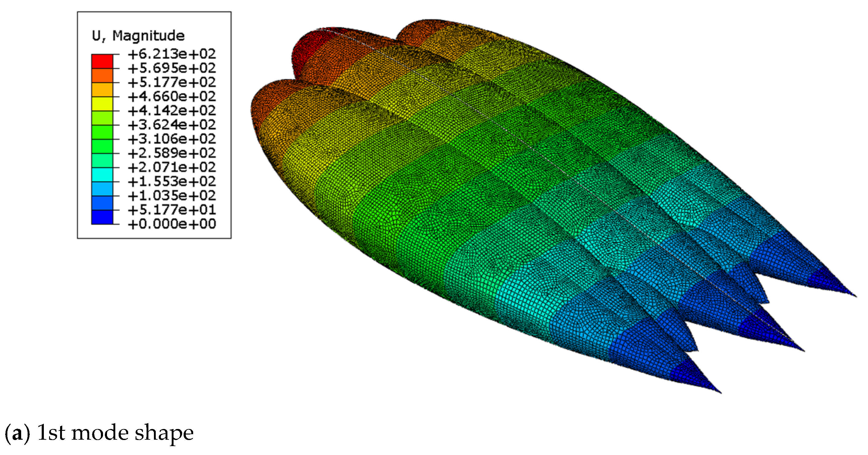
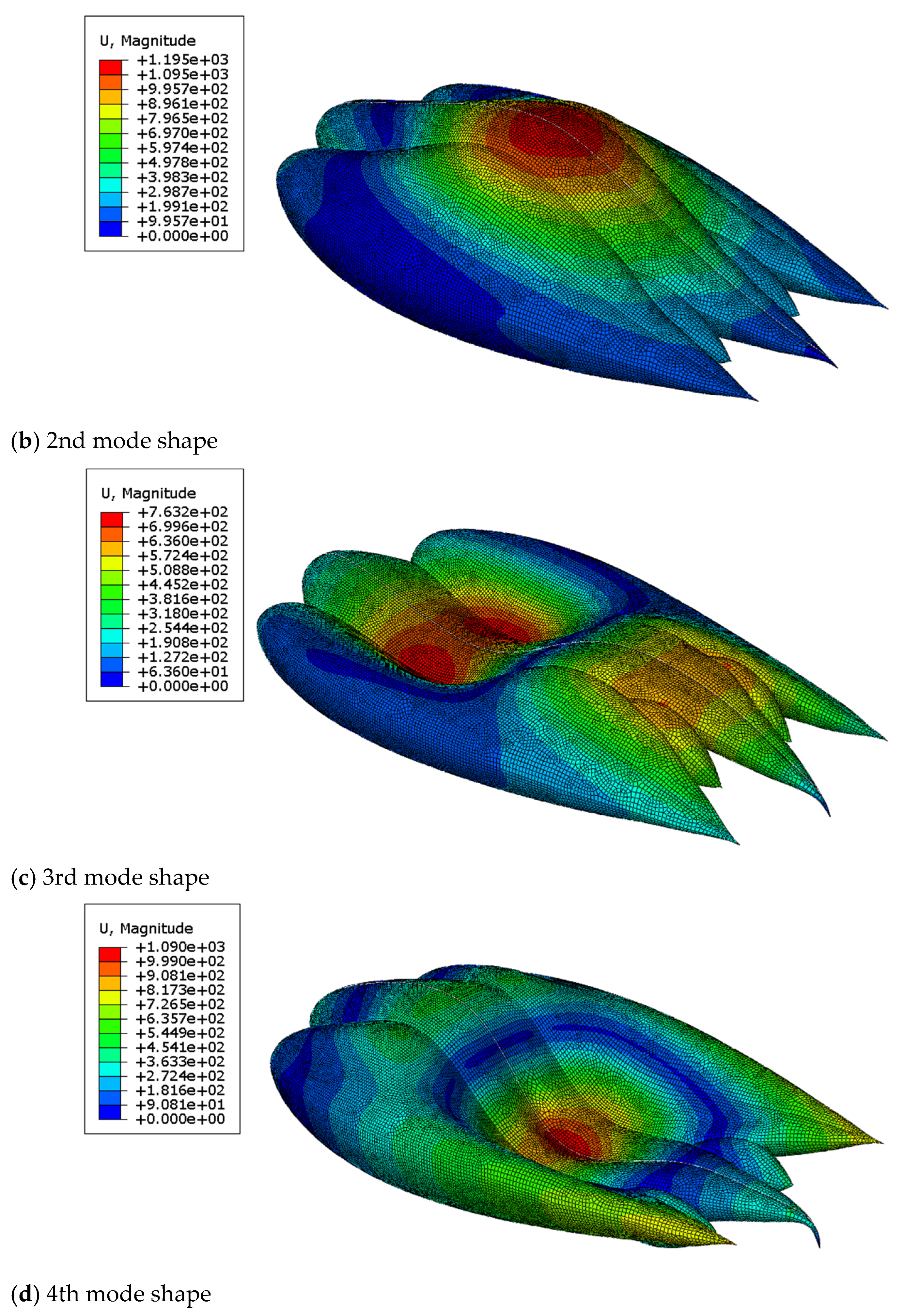
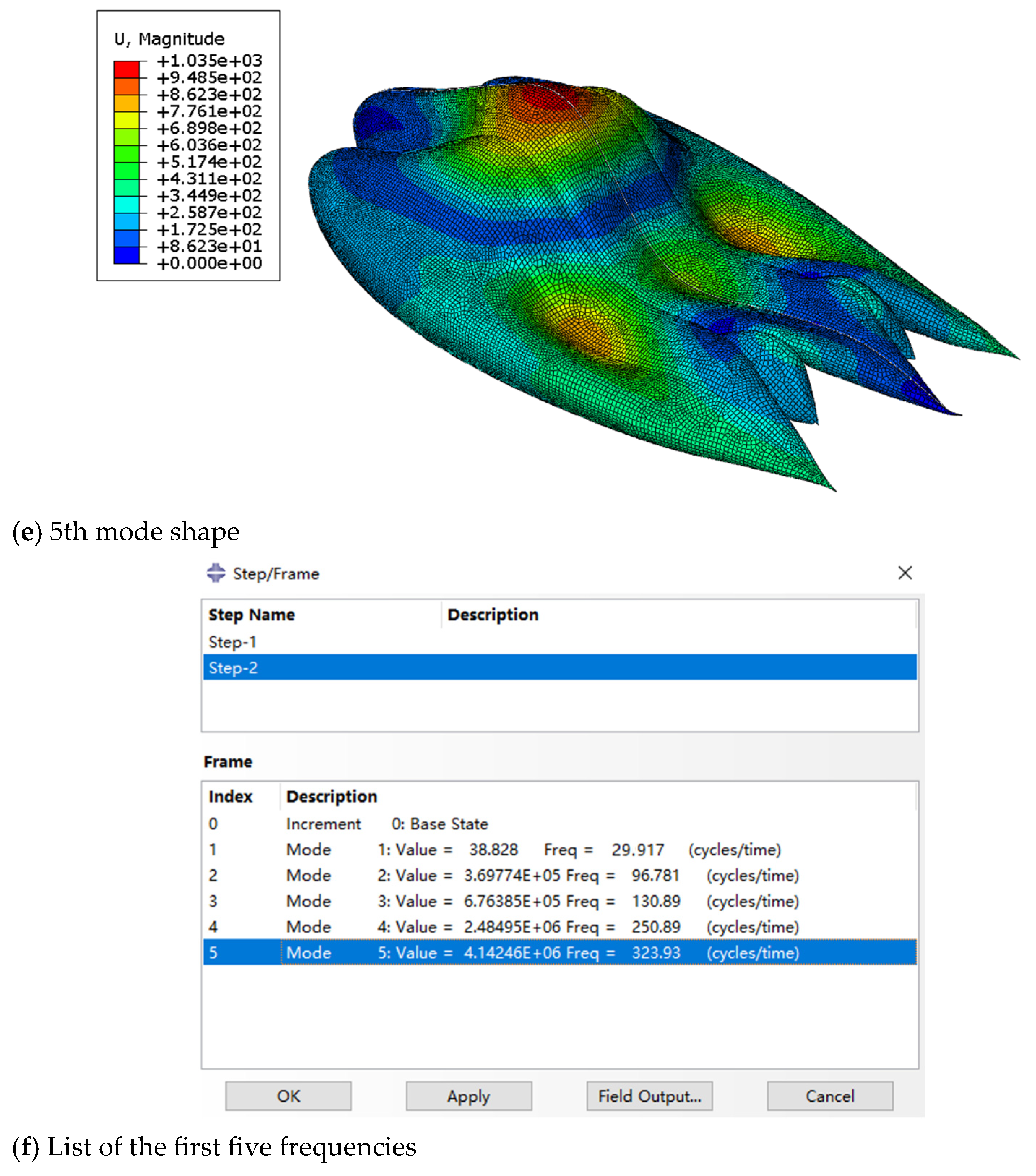
The corresponding mode shape plots of the first five modes are shown in Figure 2.

From the mode shape plots in Figure 2, it can be observed that as the modal frequency increases, the corresponding mode shapes change significantly. The first-order mode exhibits longitudinally symmetric bending, with the maximum displacement occurring at the nose. The maximum displacement is +6.213 × 10², indicating substantial overall flexible deformation. In the second-order mode, the vibration pattern transitions to transverse antisymmetric bending, with amplitude extremes concentrated on the two sides and the middle airfoil section. The deformation scale factor decreases to +1.195 × 10³, suggesting stress concentration in regions of local stiffness variation. The third-order mode presents a coupled torsion-bending vibration pattern, with evident torsional deformation in the middle region, indicating structural coupling between the envelope and the internal skeleton. In the fourth-order mode, local high-order bending dominates, with amplitude extremes concentrated in the middle of the airship; the frequency jumps to 250.89 Hz, implying relatively low structural stiffness in the middle section. The fifth-order mode exhibits a multi-node vibration pattern with discrete amplitude distribution, and high-frequency flutter occurs at the connection between the tail and the airbag, reflecting dynamic discontinuity in the appendage structure.

In summary, the modal characteristics of this hybrid airship show significant order correlation. The vibration pattern transitions from global to local modes, and the amplitude distribution is dominated by the non-uniformity of the structural stiffness.

4.2. Identification Results and Validation

Based on the simulated parameters obtained from the hybrid airship structural model and with reference to the literature, the free response function of the airship structure with additive sensor noise can be expressed as follows:

$$q(t)={\displaystyle \sum _{i=1}^5{a}_i{e}^{-{\sigma }_{i}t}\sin ({\omega }_{mdi}t+{\theta }_i)}+{\nu }_{kG}$$

(33)

where ω_mdi = 2πf_i, and f_i is the i-th intrinsic damping frequency. To simulate a general online identification scenario, the modal coefficients and phase angles of each measurement point are set randomly. The sampling frequency is 100 Hz, and the number of test points is 5. To simulate realistic sensor noise, zero-mean Gaussian white noise $v_{kG}\sim \mathcal{N}\left(0,{\sigma }_v^2\right)$ is added to the free response signals. The noise level is quantified by the signal-to-noise ratio (SNR) of the simulated acceleration signals. In this study, the noise variance ${\sigma }_v^2$ is selected such that the resulting SNR is approximately 20 dB, which is consistent with typical vibration sensor noise characteristics in operational conditions. To reduce the influence of random noise on the identification results, each simulation is repeated 50 times with independent noise realizations, and the reported identified modal parameters represent the statistical averages across these runs.

In the present numerical simulation, five virtual acceleration sensors are arranged along the longitudinal symmetry plane of the hybrid airship. Specifically, the sensors are located at the nose (10% of total length), the maximum cross-section (50% of total length), the tail (90% of total length), and two additional points at 30% and 70% of the total length along the upper surface of the main envelope. This configuration ensures coverage of the primary deformation regions identified from the first five mode shapes (Figure 2), including the nose-dominated bending in the first mode and the midsection concentration in higher-order modes.

The selection of five measurement points is supported by existing studies on flexible membrane structures. Zhang et al. [28] demonstrated that the SSI-FFT combined method can achieve reliable modal identification of biaxial tensioned membranes with only four measuring points due to the limited space of the vacuum tank, confirming that limited strategically placed sensors are sufficient for SSI-based output-only analysis. In the present case, five points provide even greater spatial coverage than the reference configuration, which enhances the reliability of the identified mode shapes while maintaining computational efficiency.

The measurement procedure consists of three steps, following the standard framework for output-only modal analysis [29]. First, acceleration responses are numerically simulated at the five virtual sensor locations under band-limited white noise excitation, with a sampling frequency of 100 Hz. Second, the simulated acceleration time histories are contaminated with zero-mean Gaussian white noise to achieve a signal-to-noise ratio of approximately 20 dB, representing typical vibration sensor noise characteristics in operational conditions. Third, the noisy response data are processed through the covariance-driven stochastic subspace identification algorithm described in Section 3.2 to extract the system matrices and subsequently the modal parameters. To reduce the influence of random noise, each simulation is repeated 50 times with independent noise realizations, and the reported results are statistical averages. This three-step procedure—data collection, system identification, and modal parameter estimation—is the standard workflow for stochastic subspace identification in operational modal analysis.

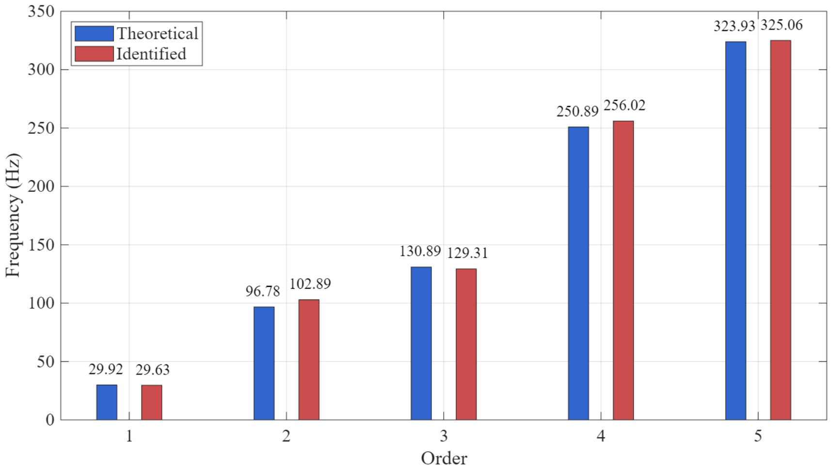
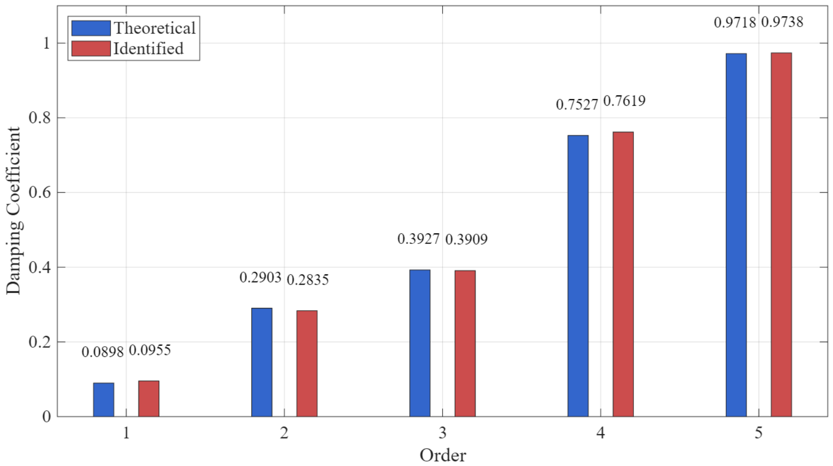
The identified modal parameters and their errors relative to the theoretical values (the simulated signal modal parameters) are presented in

Table 5. Identified modal frequencies of the first five modes and comparison with theoretical values.

	Frequency 1 (Hz)	Frequency 2 (Hz)	Frequency 3 (Hz)	Frequency 4 (Hz)	Frequency 5 (Hz)
theoretical value	29.917	96.781	130.89	250.89	323.93
identified value	29.633	102.89	129.31	256.02	325.06
inaccuracies	0.95%	6.31%	1.21%	2.04%	0.35%

and

Table 6. Identified damping coefficients of the first five modes and comparison with theoretical values.

	Damping Factor 1	Damping Factor 2	Damping Factor 3	Damping Factor 4	Damping Factor 5
theoretical value	0.0898	0.2903	0.3927	0.7527	0.9718
identified value	0.0955	0.2835	0.3909	0.7619	0.9738
inaccuracies	6.35%	2.34%	0.46%	1.22%	0.21%

and illustrated in Figure 3 and Figure 4.

As shown in Table 5 and Table 6 and Figure 3 and Figure 4, the maximum error between the theoretical and identified modal parameters (first five orders) is only 6.35% (6.31% for the second-order frequency and 6.35% for the first-order damping coefficient). This indicates excellent consistency with the theoretical model and confirms the robustness, high accuracy, and reliability of the proposed identification method. The errors exhibit certain regularity across different orders, which warrants further analysis of their sources.

The primary source of the observed errors is the additive Gaussian white noise incorporated into the free response function (Equation (33)). Measurement noise is a well-recognized source of bias and variance errors in operational modal analysis using SSI. Reynders et al. [30] demonstrated that modal parameters estimated from ambient vibration measurements are always subject to bias and variance errors, and that these errors can be quantified via first-order sensitivity of the estimates to perturbations of the output-only data.

In the present simulation, the signal-to-noise ratio is implicitly determined by the amplitude of the noise term, and the 6.35% maximum error falls within the range typically observed in SSI-based identification under moderate noise levels. Pourgholi et al. [31] reported that the average error in damping ratio estimation can be as high as 20% in seismic applications. Tondreau and Deraemaeker [32] further pointed out that uncertainty in eigenfrequencies and damping coefficients may exhibit non-normal distribution when uncorrelated noise is added at sensor locations prior to operational modal analysis. Given that damping estimation is inherently more sensitive to noise and modeling uncertainties than frequency estimation—a phenomenon extensively documented in the literature—the 6.35% maximum error observed for the airship structure is considered acceptable for engineering practice.

The discrepancy is more pronounced for the second-order frequency (6.31%) and the first-order damping coefficient (6.35%) than for the higher-order modes. This phenomenon can be explained by two factors. First, the sampling frequency is set at 100 Hz, and the number of test points is 5. While sufficient for basic identification, these settings may not be optimized for capturing lower-order modes with higher accuracy. Rainieri and Fabbrocino [33] investigated the influence of model order and the number of block rows on the accuracy of SSI estimates, concluding that the variability of modal parameter estimates is due not only to environmental factors but also to the performance of the estimator itself. Second, the modal coefficients and phase angles of each measurement point are set randomly to simulate general online identification scenarios, which introduces additional variability. The higher-order modes exhibit smaller errors because their modal characteristics are more distinct and less susceptible to overlap with noise-induced spurious modes—a trend consistent with the observations in similar numerical validation studies.

To provide a broader context for the performance of the proposed method, a qualitative comparison is made with frequency domain operational modal analysis techniques, such as frequency domain decomposition (FDD) and the peak picking (PP) method. Extensive comparative studies [26,33] have shown that for flexible structures with closely spaced modes and moderate noise levels, stochastic subspace methods consistently outperform frequency domain methods in terms of damping estimation accuracy, mode separation, and resistance to noise-induced spurious modes. Given that our airship model also exhibits moderate frequency spacing and the noise level is typical (SNR ≈ 20 dB), it is reasonable to expect that SSI would retain a similar advantage. However, a rigorous head-to-head benchmark using the same simulation dataset is beyond the scope of the present work and will be addressed in a future methodological comparison study.

5. Conclusions

In this study, the modal characteristics of a multi-airbag hybrid airship are systematically investigated through theoretical modeling, numerical simulation, and parameter identification. The main conclusions are as follows:

(1)

The theoretical model of SSI is established, and the complete identification procedure for the modal parameters of the airship structure is derived in detail. The system matrices of the airship are accurately identified. Combined with the physical relationship between modal parameters and the structural model, this method provides an effective mathematical tool for accurate modal identification of flexible airships.

(2)

Using FE software, the first five modal parameters of the hybrid airship are simulated. The modal frequencies, damping coefficients, and modal shapes are obtained, and the modal characteristics are analyzed in depth. It is found that the mode shapes exhibit significant order correlation, and the amplitude distribution is dominated by the non-uniformity of structural stiffness. These findings provide an important reference for the optimization of airship structural design.

(3)

Based on the simulated parameters and the proposed identification method, the modal parameters are identified and compared with the theoretical values. The results show excellent agreement, with a maximum relative error of only 6.35%. This verifies the robustness, high accuracy, and reliability of the proposed method. The identified parameters provide high-confidence data support for structural optimization, vibration control, and health monitoring of airships. The method is particularly suitable for lightweight airship structures that are sensitive to low-frequency modes.

The present study is based on a scaled numerical model. While the proposed identification method is validated on this model, its direct application to full-scale airships would require careful consideration of the following factors: (1) the much lower frequency range of full-scale structures, which necessitates lower sampling rates and longer data windows; (2) the increased complexity of real-world excitation compared to the idealized white noise assumed in this study; and (3) the potential presence of additional structural nonlinearities in full-scale flexible airships. These aspects will be addressed in future work involving full-scale numerical simulations or experimental tests.

References

1. Hao, J.A.; Jiang, C.W.; Gao, Z.X.; Li, C.X. Analysis of Research Progress on Aerodynamic Configuration Design of Near-Space Airships in Foreign Countries. Aeronaut. Missile 2013, 11, 53–59. [Google Scholar] [CrossRef]
2. Zhang, J.N. Research Status of Lockheed Martin’s High Altitude Hybrid Airship Project. Space Int. 2016, 5, 59–63. [Google Scholar]
3. Yan, F.; Jiang, L.H.; Cui, Y.X. Aerodynamic Performance Analysis of Layout of Airship Hull. Comput. Simul. 2014, 31, 97–102. [Google Scholar]
4. Wang, H.; Li, Z.B. Dynamic Model and Attitude Control for Airship Under the Atmospheric Turbulence. Aerosp. Control Appl. 2017, 43, 43–49. [Google Scholar] [CrossRef]
5. Rishmawi, S.; Rodriguez, S.; Chinesta, F.; Gosselin, F.P. Harmonic-modal hybrid frequency approach for parameterized non-linear dynamics. Comput. Struct. 2024, 301, 107461. [Google Scholar]
6. Li, G.S.; Liu, Z.L.; Lin, S.C.; Zhuang, Z. Static and Dynamic Mechanics Analysis for a Large-Scale Rigidity-Flexibility Airship Structure. Eng. Mech. 2015, 32, 219–228. [Google Scholar]
7. Yang, Y.N.; Zheng, W.; Yan, Y.; Shao, H.B. Flight mode analysis for stratospheric airships. J. Natl. Univ. Def. Technol. 2015, 37, 57–64. [Google Scholar]
8. Zhang, X.; Zhao, Q.; Ma, L.; Zhang, K. Frequency-domain analyses on the aeroelastic characteristics of thrust-vectored system on airship. Aerosp. Sci. Technol. 2021, 116, 106853. [Google Scholar]
9. Yang, Y.N. Dynamics Modeling and Flight Control for a Stratospheric Airship. Ph.D. Thesis, National University of Defense Technology, Changsha, China, 2013. [Google Scholar]
10. Huang, Y.D.; Xu, J.F. Dynamic modeling and control system design of unmanned airship. Flight Dyn. 2025, 43, 34–41. [Google Scholar]
11. Sadeghzadeh, S.; Khatibi, M.M. Modal identification of single layer graphene nano sheets from ambient responses using frequency domain decomposition. Eur. J. Mech. A-Solids 2017, 65, 70–78. [Google Scholar] [CrossRef]
12. Long, F.; Huang, L.T.; Jiang, W. Overall Design and Performance Analysis of a Conventional Airship and a Hybrid Airship. Adv. Aeronaut. Sci. Eng. 2012, 2, 150–155. [Google Scholar]
13. Le, T.-P.; Argoul, P. Modal identification using the frequency-scale domain decomposition technique of ambient vibration responses. J. Sound Vib. 2016, 384, 325–338. [Google Scholar] [CrossRef]
14. Wang, T.; Ren, W.X.; Yang, D.; He, W.Y. Asynchronously measured bridge modal identification based on stochastic subspace method. J. Hefei Univ. Technol. (Nat. Sci.) 2023, 46, 333–340. [Google Scholar]
15. Charbonnel, P.-É. Assessing the performance of subspace-based modal identification procedures for systems subjected to structural damage and Coulomb-friction non-linearities. Mech. Syst. Signal Proc. 2023, 199, 110399. [Google Scholar]
16. Gustavo, W.; Roberta, L.; Rubens, S. Modal identification of a light and flexible wind turbine blade under wind excitation. J. Eng. Math. 2022, 133, 3. [Google Scholar] [CrossRef]
17. Singh, S.; Danish, M.; Saha, K.; Singh, B.N. Numerical simulation and analysis of fluid-structure interaction on 3D MHKF-180 and NACA4418 cavitating hydrofoils. Ocean Eng. 2023, 272, 113867. [Google Scholar] [CrossRef]
18. Omadjohwoefe, O.S. Hybrid Air Vehicles announces launch customer for Airlander 10. Engineer (Online Ed.) 2022, 1. [Google Scholar]
19. Excell, J. BUOYANT FUTURE: After a spell out of the limelight, UK aerospace pioneer Hybrid Air Vehicles, believes the time is now right for a lighter than air transport revolution. Engineer 2021, 302, 26–28. [Google Scholar]
20. Zhou, W.; Zhong, L.; Kang, W.; Xu, Y.; Luan, C.; Fu, J. Modal parameter identification of electric spindles based on covariance-driven stochastic subspace. Machines 2024, 12, 774. [Google Scholar] [CrossRef]
21. Luo, J.; Kang, J.; Sun, J.B.; Zeng, S.H. Uncertainty quantification based on a covariance-driven stochastic subspace method. J. Vib. Shock 2024, 43, 272–279. [Google Scholar]
22. Sun, S.; Yang, B.; Zhang, Q.; Wüchner, R.; Pan, L.; Zhu, H. Fast online implementation of covariance-driven stochastic subspace identification. Mech. Syst. Signal Proc. 2023, 197, 110326. [Google Scholar] [CrossRef]
23. Li, Z.; Fu, J.; Liang, Q.; Mao, H.; He, Y. Modal identification of civil structures via covariance-driven stochastic subspace method. Math. Biosci. Eng. 2019, 16, 5709–5728. [Google Scholar] [CrossRef] [PubMed]
24. Khan, I.; Shan, D.; Li, Q. Continuous Modal Parameter Identification of a Cable-Stayed Bridge Based on Robustious Decomposition and Covariance-Driven Stochastic Subspace Identification. IJST-T Civ. Eng. 2016, 40, 11–22. [Google Scholar]
25. Reynders, E.P.B. Uncertainty quantification in data-driven stochastic subspace identification. Mech. Syst. Signal Proc. 2021, 151, 107338. [Google Scholar] [CrossRef]
26. Reynders, E. System identification methods for (operational) modal analysis: Review and comparison. Arch. Comput. Methods Eng. 2012, 19, 51–124. [Google Scholar] [CrossRef]
27. Peeters, B.; De Roeck, G. Stochastic system identification for operational modal analysis: A review. J. Dyn. Syst. Meas. Control 2001, 123, 659–667. [Google Scholar] [CrossRef]
28. Zhang, Y.B.; Zhao, B.; Hu, J.H.; Chen, W.J.; Deng, X.W.; Yu, Z.Y.; Xie, C.; Peng, F.J. Modal identification experimental investigations and calculation method for biaxial tensioned membranes. Thin-Walled Struct. 2020, 154, 106877. [Google Scholar] [CrossRef]
29. Peeters, B.; De Roeck, G. Reference-based stochastic subspace identification for output-only modal analysis. Mech. Syst. Signal Process. 1999, 13, 855–878. [Google Scholar]
30. Edwin, R.; Rik, P.; Guido, D.R. Uncertainty bounds on modal parameters obtained from stochastic subspace identification. Mech. Syst. Signal Process. 2008, 22, 948–969. [Google Scholar] [CrossRef]
31. Pourgholi, M.; Ghannadi, M.; Gavgani, S.S. Modal analysis of earthquake records for dams using stochastic subspace based on error analysis. Eng. Rep. 2024, 6, e12822. [Google Scholar]
32. Tondreau, G.; Deraemaeker, A. Numerical and experimental analysis of uncertainty on modal parameters estimated with the stochastic subspace method. J. Sound Vib. 2014, 333, 4376–4401. [Google Scholar] [CrossRef]
33. Rainieri, C.; Fabbrocino, G. Influence of model order and number of block rows on accuracy and precision of modal parameter estimates in stochastic subspace identification. Int. J. Lifecycle Perform. Eng. 2014, 1, 317. [Google Scholar] [CrossRef]
Figure 1. Structural model of the multi-airbag hybrid configuration airship.
Aerospace 13 00609 g001
Figure 2. Mode shapes of the first five modes of the hybrid airship.
Aerospace 13 00609 g002aAerospace 13 00609 g002bAerospace 13 00609 g002c
Figure 3. Comparison of identified and theoretical modal frequencies for the first five modes.
Aerospace 13 00609 g003
Figure 4. Comparison of identified and theoretical damping coefficients for the first five modes.
Aerospace 13 00609 g004