Author Contributions
Conceptualization, R.H. and Q.W.; methodology, H.P.; software, J.L.; validation, H.P., R.H., and J.L.; formal analysis, Q.W.; investigation, H.P.; resources, H.P.; data curation, R.H.; writing original draft preparation, R.H.; review and editing, Q.W.; visualization, J.L.; supervision, Q.W.; project administration, H.P.; funding acquisition, H.P. All authors have read and agreed to the published version of the manuscript.
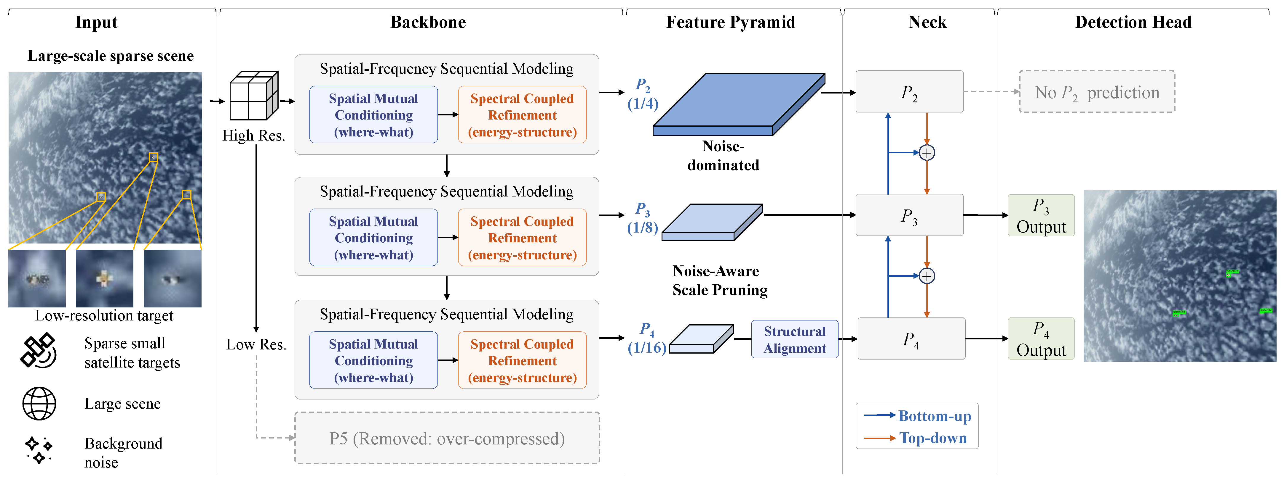
Figure 1.
Overview of the proposed Decoupling-Refinement Spatial–Spectral Network (DRSS-Net) for satellite object detection. The framework is built upon a YOLOv12-style architecture with a redesigned backbone and scale-aware structural adaptation. Specifically, the deepest feature level () is removed to avoid excessive spatial compression, while the shallow level () is excluded from prediction due to noise dominance but still participates in feature aggregation through the neck. The backbone is composed of cascaded spatial–spectral modules, where spatial mutual conditioning improves feature identifiability by modeling where–what coupling, and spectral coupled refinement enhances structural consistency via frequency-domain interaction. The neck employs bidirectional feature aggregation, and the detection head produces predictions only at intermediate scales ( and ), achieving a balance between robustness and efficiency.
Figure 1.
Overview of the proposed Decoupling-Refinement Spatial–Spectral Network (DRSS-Net) for satellite object detection. The framework is built upon a YOLOv12-style architecture with a redesigned backbone and scale-aware structural adaptation. Specifically, the deepest feature level () is removed to avoid excessive spatial compression, while the shallow level () is excluded from prediction due to noise dominance but still participates in feature aggregation through the neck. The backbone is composed of cascaded spatial–spectral modules, where spatial mutual conditioning improves feature identifiability by modeling where–what coupling, and spectral coupled refinement enhances structural consistency via frequency-domain interaction. The neck employs bidirectional feature aggregation, and the detection head produces predictions only at intermediate scales ( and ), achieving a balance between robustness and efficiency.
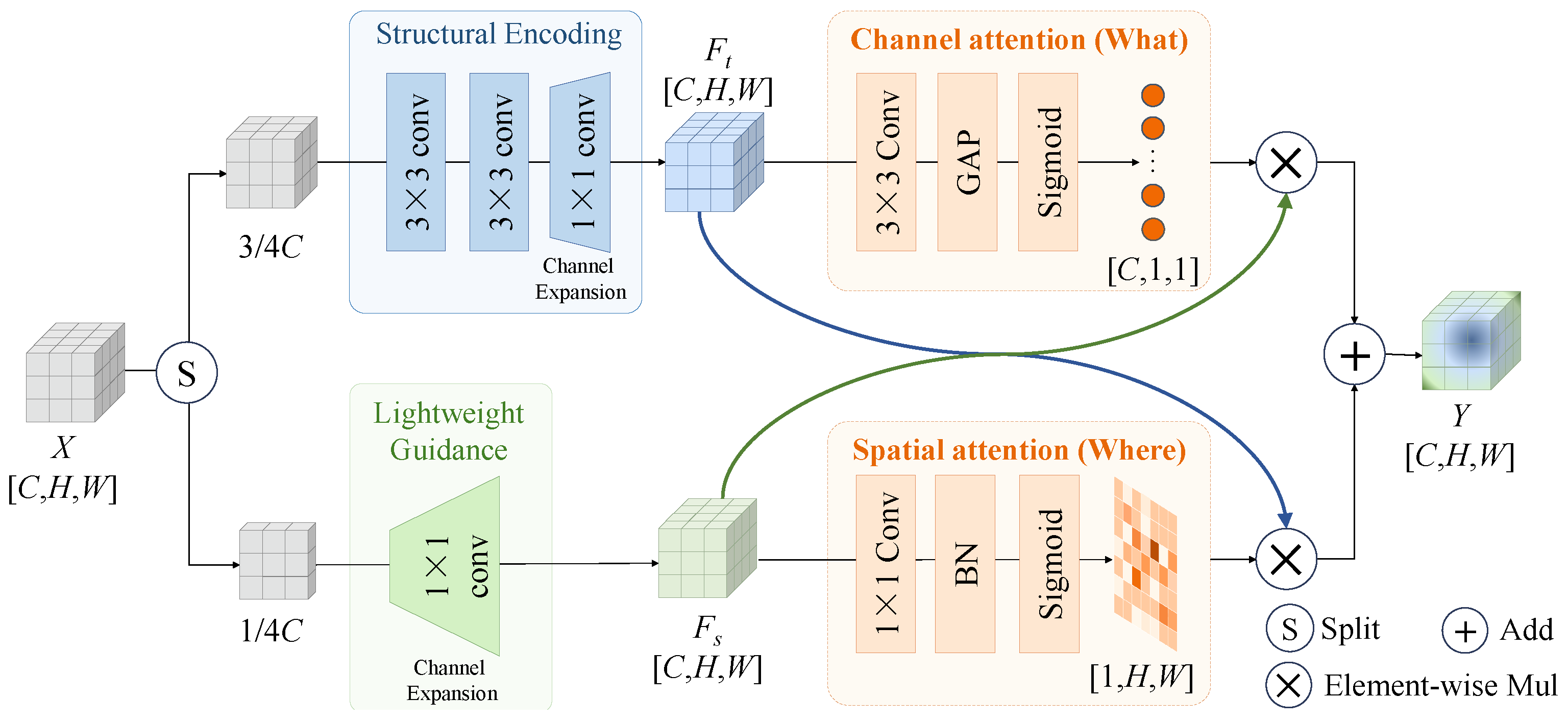
Figure 2.
Illustration of the spatial component of DRSS-Net: spatial mutual conditioning (SMC). The module follows a decoupling-refinement paradigm, where where–what interaction is modeled through mutual conditioning to enhance feature discriminability and structural alignment.
Figure 2.
Illustration of the spatial component of DRSS-Net: spatial mutual conditioning (SMC). The module follows a decoupling-refinement paradigm, where where–what interaction is modeled through mutual conditioning to enhance feature discriminability and structural alignment.
Figure 3.
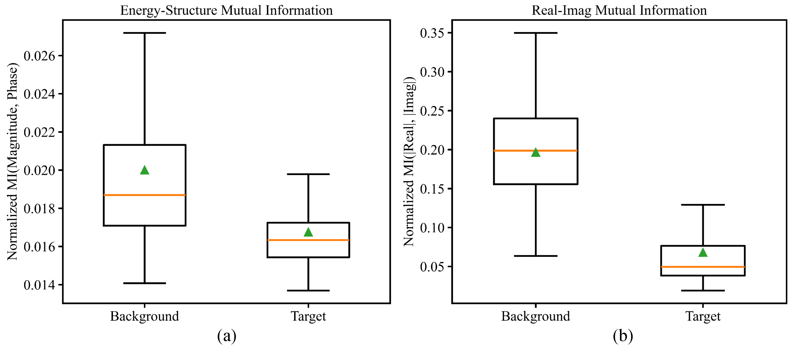
Mutual information analysis of background and target patches under different spectral representations. Box plots show the distributions of normalized mutual information for (a) energy–structure (magnitude–phase) and (b) real–imaginary representations. The orange line represents the median, while the green triangle indicates the mean.
Figure 3.
Mutual information analysis of background and target patches under different spectral representations. Box plots show the distributions of normalized mutual information for (a) energy–structure (magnitude–phase) and (b) real–imaginary representations. The orange line represents the median, while the green triangle indicates the mean.
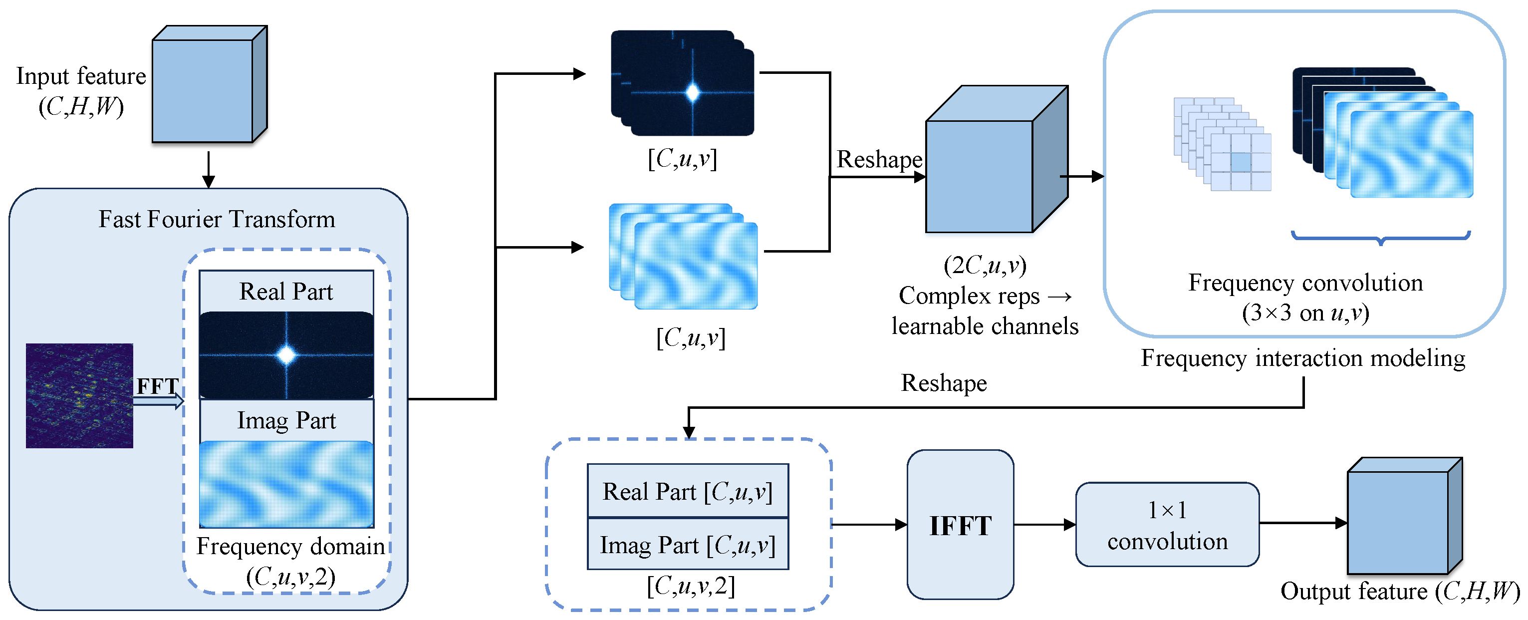
Figure 4.
Illustration of the spectral component of DRSS-Net: spectral coupled refinement. The module follows a decoupling-refinement paradigm in the frequency domain, where energy–structure interaction is modeled through coupled refinement to enhance representation stability.
Figure 4.
Illustration of the spectral component of DRSS-Net: spectral coupled refinement. The module follows a decoupling-refinement paradigm in the frequency domain, where energy–structure interaction is modeled through coupled refinement to enhance representation stability.
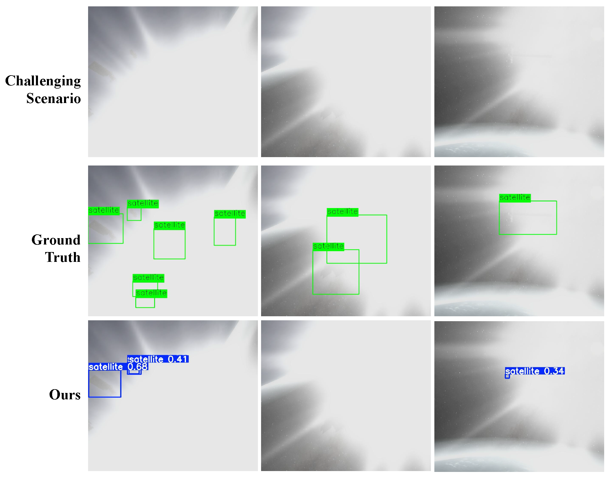
Figure 5.
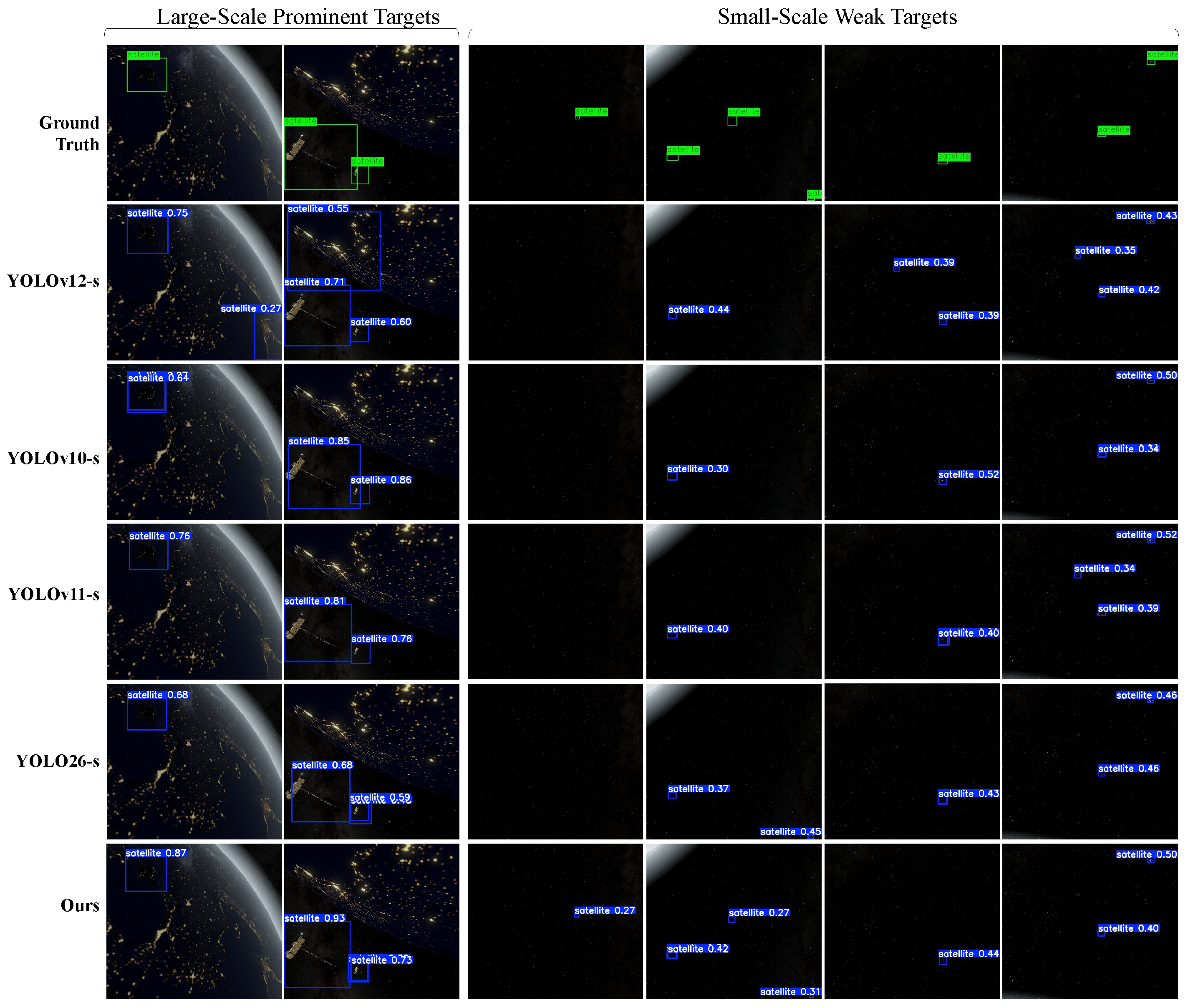
Qualitative comparison of challenging scenarios. The first two columns show large-scale prominent targets, where most methods perform comparably. The last four columns present small-scale weak targets under complex backgrounds, where baseline methods suffer from missed detections and false alarms, while the proposed method achieves more accurate and complete detection. The blue boxes represent the detected targets, while the green boxes indicate the ground-truth annotations.
Figure 5.
Qualitative comparison of challenging scenarios. The first two columns show large-scale prominent targets, where most methods perform comparably. The last four columns present small-scale weak targets under complex backgrounds, where baseline methods suffer from missed detections and false alarms, while the proposed method achieves more accurate and complete detection. The blue boxes represent the detected targets, while the green boxes indicate the ground-truth annotations.
Figure 6.
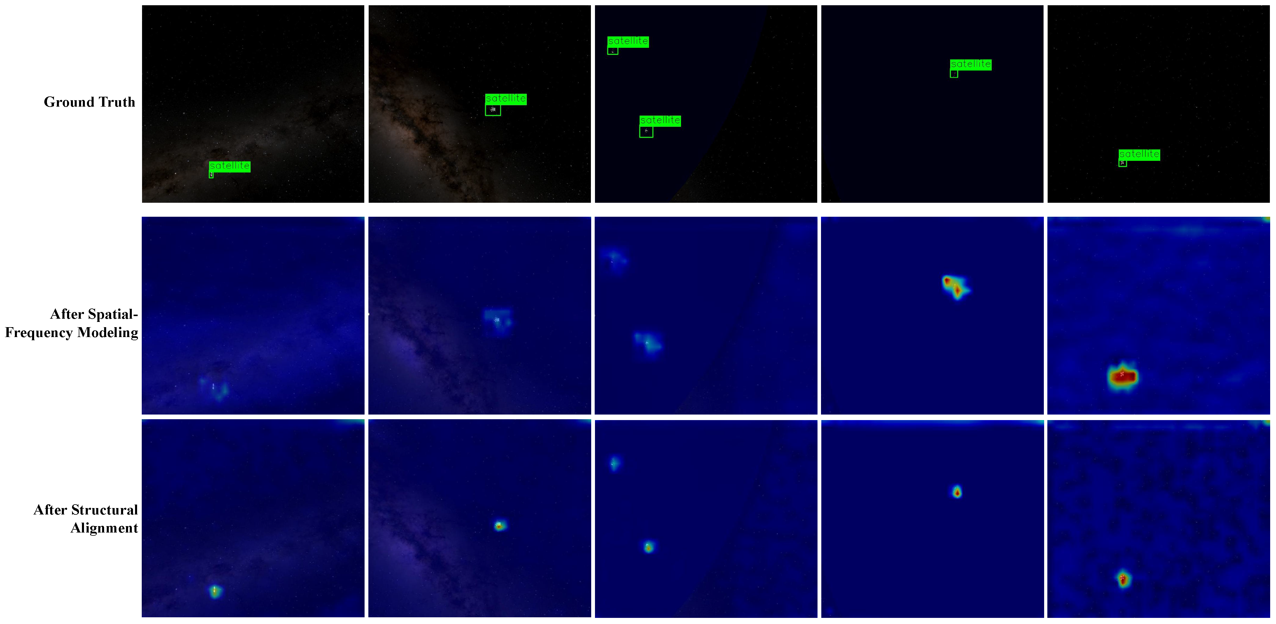
Visualization of feature evolution at different stages. From top to bottom: ground truth, features after spatial-frequency modeling, and features after structural alignment. It can be observed that target responses become progressively more salient, while background interference is gradually suppressed, leading to improved localization consistency. The color map represents the feature intensity, with warmer colors indicating higher activation values and cooler colors indicating lower values.
Figure 6.
Visualization of feature evolution at different stages. From top to bottom: ground truth, features after spatial-frequency modeling, and features after structural alignment. It can be observed that target responses become progressively more salient, while background interference is gradually suppressed, leading to improved localization consistency. The color map represents the feature intensity, with warmer colors indicating higher activation values and cooler colors indicating lower values.
Figure 7.
Detection results under extreme bright-star interference. The target response is partially overwhelmed by strong stellar emissions, resulting in a missed detection. The blue boxes represent the detected targets, while the green boxes indicate the ground-truth annotations.
Figure 7.
Detection results under extreme bright-star interference. The target response is partially overwhelmed by strong stellar emissions, resulting in a missed detection. The blue boxes represent the detected targets, while the green boxes indicate the ground-truth annotations.
Table 1.
Comparison with state-of-the-art object detectors on the SODv2. The proposed method achieves the best trade-off across all evaluation metrics while maintaining a lightweight model size and computational cost.
Table 1.
Comparison with state-of-the-art object detectors on the SODv2. The proposed method achieves the best trade-off across all evaluation metrics while maintaining a lightweight model size and computational cost.
| Scale | Model | Precision | Recall | mAP@50 | mAP@50-95 | Params | FLOPs | FPS |
|---|
| | | (%) | (%) | (%) | (%) | | | |
|---|
| Small | YOLOv8-s | 76.77 | 72.32 | 71.76 | 26.82 | 11.13 M | 28.4 G | 101.65 |
| YOLOv9-s | 68.33 | 69.10 | 69.51 | 25.92 | 7.17 M | 26.7 G | 40.99 |
| YOLOv10-s | 69.12 | 62.66 | 69.40 | 25.93 | 7.22 M | 21.4 G | 83.94 |
| YOLOv11-s | 73.05 | 70.97 | 70.67 | 25.69 | 9.41 M | 21.3 G | 85.14 |
| YOLOv12-s | 75.69 | 73.82 | 73.01 | 27.64 | 9.23 M | 21.2 G | 50.94 |
| YOLO26-s | 64.09 | 66.52 | 65.80 | 24.62 | 9.47 M | 20.5 G | 66.28 |
| L-FFCA-YOLO | 67.20 | 66.50 | 61.70 | 19.50 | 5.04 M | 37.1G | 91.01 |
| FBRT-YOLO | 74.10 | 74.20 | 74.00 | 27.30 | 7.36 M | 58.7 G | 111.00 |
| FFCA-YOLO | 71.00 | 63.10 | 62.10 | 20.70 | 7.12 M | 51.2 G | 70.87 |
| Medium | YOLOv11-m | 72.07 | 70.87 | 69.55 | 27.51 | 20.03 M | 67.6 G | 59.43 |
| YOLOv12-m | 68.49 | 72.75 | 72.21 | 26.93 | 20.11 M | 67.1 G | 38.00 |
| YOLO26-m | 68.95 | 69.53 | 69.29 | 25.88 | 20.35 M | 67.8 G | 66.22 |
| RTDETR-r18 | 72.71 | 72.02 | 71.95 | 26.01 | 19.87 M | 56.9 G | 33.22 |
| CSFPR-RTDETR | 70.90 | 68.70 | 70.40 | 25.00 | 14.08 M | 63.8 G | 45.2 |
| Large | YOLOv11-l | 75.74 | 78.11 | 75.92 | 27.73 | 25.28 M | 86.6 G | 40.90 |
| YOLOv12-l | 73.54 | 69.19 | 69.36 | 26.50 | 26.34 M | 88.5 G | 30.84 |
| YOLO26-l | 72.98 | 64.38 | 67.17 | 24.20 | 24.75 M | 86.1 G | 36.64 |
| RTMDet | 67.37 | 70.50 | 69.10 | 28.30 | 24.20 M | 39.2 G | – |
| HRNet | 73.44 | 71.30 | 74.50 | 27.20 | 23.00 M | 38.3 G | – |
| Xlarge | YOLOv11-x | 71.56 | 73.45 | 73.01 | 27.64 | 56.83 M | 194.4 G | 40.42 |
| YOLOv12-x | 79.58 | 76.92 | 76.44 | 29.83 | 59.04 M | 198.5 G | 26.69 |
| YOLO26-x | 67.08 | 66.95 | 67.59 | 26.67 | 55.63 M | 193.4 G | 40.89 |
| – | Ours | 77.06 | 76.40 | 79.15 | 28.47 | 3.46 M | 23.0 G | 72.69 |
Table 2.
Comparison with state-of-the-art object detectors on the NCSTP dataset. The proposed method achieves the best trade-off across all evaluation metrics while maintaining a lightweight model size and computational cost.
Table 2.
Comparison with state-of-the-art object detectors on the NCSTP dataset. The proposed method achieves the best trade-off across all evaluation metrics while maintaining a lightweight model size and computational cost.
| Model | Precision | Recall | mAP@50 | mAP@50-95 | Params | FLOPs | FPS |
|---|
| | (%) | (%) | (%) | (%) | | | |
|---|
| YOLOv8-s | 98.55 | 96.92 | 98.66 | 82.27 | 11.13 M | 28.4 G | 115.80 |
| YOLOv9-s | 99.16 | 97.99 | 99.12 | 82.98 | 7.17 M | 26.7 G | 49.45 |
| YOLOv10-s | 96.24 | 97.35 | 98.60 | 81.20 | 7.22 M | 21.4 G | 83.94 |
| FBRT-YOLO-m | 98.71 | 98.11 | 99.05 | 82.54 | 7.36 M | 58.7 G | 90.32 |
| FFCA-YOLO | 97.60 | 97.20 | 99.10 | 79.60 | 7.12 M | 51.2 G | 52.73 |
| L-FFCA-YOLO | 98.50 | 97.70 | 98.50 | 76.50 | 5.04 M | 37.1 G | 46.83 |
| YOLOv11-s | 98.68 | 97.30 | 98.45 | 82.60 | 9.42 M | 21.3 G | 80.94 |
| YOLOv12-s | 97.15 | 96.80 | 98.68 | 81.87 | 9.08 M | 19.3 G | 51.92 |
| YOLOv13-s | 97.84 | 97.18 | 99.09 | 82.63 | 9.01 M | 20.1 G | 37.41 |
| YOLO26-s | 96.96 | 97.62 | 98.84 | 81.95 | 9.47 M | 20.5 G | 77.14 |
| Ours | 98.84 | 98.16 | 99.38 | 83.19 | 3.46 M | 23.0 G | 70.64 |
Table 3.
Ablation study on the effectiveness of different components. “Spatial (Backbone)” and “Spectral” denote the proposed spatial and spectral modules embedded in the backbone, respectively, while “Structural Alignment ( Neck)” denotes the additional spatial refinement applied at the level in the neck.
Table 3.
Ablation study on the effectiveness of different components. “Spatial (Backbone)” and “Spectral” denote the proposed spatial and spectral modules embedded in the backbone, respectively, while “Structural Alignment ( Neck)” denotes the additional spatial refinement applied at the level in the neck.
| Spatial | Spectral | Structural Alignment | Precision | Recall | mAP@50 | mAP@50-95 | Params | FLOPs |
|---|
| (Backbone) | (Backbone) | ( Neck) | (%) | (%) | (%) | (%) | | |
|---|
| × | × | × | 73.80 | 73.82 | 75.56 | 26.23 | 5.25 M | 35.9 G |
| ✔ | × | ✔ | 74.26 | 73.06 | 75.45 | 28.90 | 2.94 M | 20.4 G |
| ✔ | ✔ | × | 74.20 | 74.96 | 75.37 | 27.18 | 3.25 M | 22.4 G |
| ✔ | ✔ | ✔ | 77.06 | 76.40 | 79.15 | 28.47 | 3.46 M | 23.0 G |
Table 4.
Ablation study on noise-aware scale pruning. “P2 Head” indicates whether predictions are made on the level, and “P5 Layer” denotes whether the deepest feature level is retained in the backbone.
Table 4.
Ablation study on noise-aware scale pruning. “P2 Head” indicates whether predictions are made on the level, and “P5 Layer” denotes whether the deepest feature level is retained in the backbone.
| P5 Layer | P2 Head | Precision | Recall | mAP@50 | mAP@50-95 | Params | FLOPs |
|---|
| | | (%) | (%) | (%) | (%) | | |
|---|
| ✔ | × | 74.48 | 74.68 | 74.30 | 26.87 | 9.91 M | 19.2 G |
| × | ✔ | 77.18 | 71.24 | 74.68 | 27.85 | 3.62 M | 30.7 G |
| × | × | 77.06 | 76.40 | 79.15 | 28.47 | 3.46 M | 23.0 G |
Table 5.
Comparison of different frequency representations within the spectral refinement module.
Table 5.
Comparison of different frequency representations within the spectral refinement module.
| Method | Precision | Recall (%) | mAP@50 (%) | mAP@50-95 (%) | Params | FLOPs | FPS |
|---|
| Wavelet-based | 75.23 | 72.10 | 72.46 | 26.75 | 5.79 M | 25.8 G | 53.91 |
| FFT-based (Ours) | 77.06 | 76.40 | 79.15 | 28.47 | 3.46 M | 23.0 G | 72.69 |
Table 6.
Effect of spectral kernel size in the SCR module.
Table 6.
Effect of spectral kernel size in the SCR module.
| Kernel | Precision | Recall | mAP@50 | mAP@50-95 | Params | FLOPs | FPS |
|---|
| 77.06 | 76.40 | 79.15 | 28.47 | 3.46 M | 23.0 G | 72.69 |
| 82.01 | 75.54 | 77.15 | 27.95 | 4.84 M | 28.2 G | 64.01 |
| 75.03 | 73.51 | 71.80 | 28.01 | 6.91 M | 36.0 G | 53.48 |
Table 7.
Robustness analysis of the proposed method across three independent runs on the SODv2 dataset.
Table 7.
Robustness analysis of the proposed method across three independent runs on the SODv2 dataset.
| Metric | Run 1 | Run 2 | Run 3 | Mean ± Std |
|---|
| Precision (%) | 77.06 | 76.88 | 77.84 | |
| Recall (%) | 76.40 | 75.18 | 76.09 | |
| mAP@50 (%) | 79.15 | 78.06 | 78.17 | |
| mAP@50-95 (%) | 28.47 | 28.16 | 27.88 | |
Table 8.
Robustness analysis and statistical significance of the proposed method compared to YOLOv12 on SODv2 across three independent runs.
Table 8.
Robustness analysis and statistical significance of the proposed method compared to YOLOv12 on SODv2 across three independent runs.
| Metric | Baseline (Mean) | Ours (Mean) | Improvement | Welch t-Test p-Value | Significant (p < 0.05) |
|---|
| Precision (%) | 74.77 | 77.26 | 2.49 | 0.0261 | Yes |
| Recall (%) | 73.15 | 75.89 | 2.74 | 0.0095 | Yes |
| mAP@50 (%) | 74.24 | 78.46 | 4.22 | 0.0093 | Yes |
| mAP@50-95 (%) | 27.14 | 28.17 | 1.03 | 0.0496 | Yes |