Dynamic Modeling and Thermo-Mechanical Coupling Analysis of Variable-Geometry Spacecraft Antenna with Clearance Hinges Under Extreme Thermal Environment

Abstract

Extreme cyclic temperature fluctuations (−200 °C to 200 °C) and inherent clearance nonlinearity in deployment hinges severely threaten the on-orbit deployment accuracy and dynamic stability of large variable-geometry spacecraft antennas for geosynchronous Earth orbit applications. However, current modeling approaches suffer from three critical limitations: single-configuration models requiring manual switching, there are inherent geometric nonlinear errors from conventional floating frame formulations, and incomplete thermo-mechanical coupling neglects the temperature effects on contact stiffness and friction. To address these gaps, we propose a unified high-fidelity dynamic model based on the Absolute Nodal Coordinate Formulation (ANCF). This model eliminates geometric errors and mesh mismatch, enables seamless multi-configuration deployment without switching, and fully incorporates temperature-dependent material properties and nonlinear contact forces. An improved Hilber–Hughes–Taylor-$\alpha$ implicit integration algorithm with second-order accuracy and unconditional stability is adopted to solve the strongly nonlinear differential-algebraic equations. Numerical results demonstrate that the proposed model achieves a calculation error below 3% against experimental data, significantly outperforming the traditional floating frame of reference formulation with an error of 15–22%. Non-uniform temperature fields increase thermally induced vibration amplitudes by 32–45%, and every 0.1 increase in the friction coefficient raises the impact force at the clearance hinge by 15–20%. The proposed unified modeling framework provides a solid theoretical basis for deployment stability prediction and the on-orbit control optimization of large variable-geometry spacecraft antennas.

1. Introduction

Large variable-geometry spacecraft antennas are essential for geosynchronous earth orbit communication and remote sensing. Their deployment accuracy and dynamic stability are threatened by extreme temperature cycles from −200 °C to 200 °C and clearance nonlinearity in hinges. Most existing studies use single-configuration models with unidirectional thermal–structure coupling. A unified framework that couples temperature-dependent material properties with clearance nonlinearity across multi-stage variable-geometry deployment is lacking.

The modeling of deployable flexible structures has evolved considerably. Meguro et al. [1] characterized the on-orbit deployment of large reflectors. Zhang et al. [2] established static and dynamic frameworks for deployable structures. Tan et al. [3] developed dynamic models for large mesh reflectors, and Sun et al. [4] studied the deployment dynamics of spinning inflatable structures. Li et al. [5] first introduced joint clearance into deployable space structure dynamics, revealing its nonlinear effects. Tian et al. [6] reviewed methodologies for multibody systems with clearance joints. Chen et al. [7] proposed an efficient method for planar systems with revolute clearance joints. Guo et al. [8] studied the stiffness variation of joints under thermo-mechanical loading. Polla et al. [9] developed coupled thermo-mechanical models for composite panels under impact. Kuang et al. [10] analyzed the motion accuracy of dual-manipulator systems with clearance. Du et al. [11] studied rotor-stator clearance under multi-physical fields. Mei et al. [12] worked on deployable solar concentrators, and Wu et al. [13] analyzed the accuracy of truss antennas with clearance. Despite these efforts, a unified framework for multi-stage deployment (main boom, secondary arm, reflector) without configuration switching remains absent.

Thermo-mechanical coupling is another critical aspect. Thornton [14] established the foundational theory for aerospace thermal structures, and Boley [15] first identified thermally induced beam vibrations. For space deployable structures, Cao et al. [16] revealed thermal shock excitation mechanisms, and Shen et al. [17] quantified thermal deformation effects on antenna surface accuracy. These early works relied on the conventional floating frame of reference formulation (FFRF), which introduces inherent geometric nonlinear errors in large deformation problems.

The absolute nodal coordinate formulation (ANCF) overcame this limitation. Shen et al. [18] proposed an ANCF framework for the thermal vibration analysis of beams, inherently eliminating FFRF errors by using global position and gradient vectors. Cui et al. [19] then developed a unified thermo-mechanical description with a consistent discretization of displacement and temperature fields via identical ANCF shape functions, resolving the mesh mismatch problem. To address numerical locking, Obrezkov et al. [20] systematically evaluated locking alleviation methods for continuum ANCF beam elements, providing guidance for robust simulations. More recent studies have further extended ANCF-based thermal–dynamic analysis to flexible multibody systems and large-displacement thermal problems. Tian et al. [21] developed a free-interface component-mode-synthesis reduction strategy for thermo-mechanical coupling flexible multibody dynamics, while Yu et al. [22] applied ANCF to the thermo-mechanical coupled analysis of belt-drive systems. Tian et al. [23] formulated constrained large-displacement thermal analysis, and Abdalla et al. [24] further proposed a computational algorithm for coupled thermomechanical large-displacement problems. These studies demonstrate the suitability of ANCF-type formulations for thermal–dynamic coupling with large deformation, but they do not address deployable space antennas with clearance hinges.

At the system level, Yuan et al. [25] extended the ANCF thermo-mechanical framework to the rigid–flexible–thermal coupling of hub-multiplate systems with frictional contact, demonstrating that contact alters thermal energy distribution. Zhou et al. [26] developed an ANCF-based thermo-flexible model for composite laminated plates with anisotropic thermal conductivity and temperature-dependent properties. Related thin-walled and space-structure studies have also emphasized thermally induced vibration and rigid–flexible–thermal coupling. Sun et al. [27] modeled and controlled thermally induced vibrations of flexible plates, Li et al. [28] developed a thermoelastic ANCF deployable thin-plate model for telescopic wing systems, Zhou et al. [29] investigated rigid–flexible–thermal coupled solar panel multibody systems composed of composite laminated shells, and Ma et al. [30] analyzed thermally induced vibrations of spacecraft thin-walled composite circular tubes using higher-order ANCF beam elements. However, these studies primarily focus on transmission systems, plates, tubes, wings, or solar-array-type structures; clearance nonlinearity in deployable antenna joints was not addressed. The capability of ANCF for large deformation and contact problems is also recognized in soft robotics [31], further confirming its versatility.

The first coupling of thermo-mechanical effects with clearance nonlinearity using ANCF was performed by Li et al. [32], who analyzed planar composite solar arrays with clearance joints. They identified the thermal amplification of clearance vibrations but with limitations: a constant friction coefficient and neglected temperature effects on contact stiffness, no temperature-dependent structural mass and damping, and restriction to a single configuration without multi-stage deployment. Jin et al. [33] later studied the thermal–structural behavior of modular antenna supports without clearance nonlinearity.

Consequently, no existing ANCF-based model simultaneously incorporates temperature effects on mass, stiffness, damping, clearance contact stiffness, and friction coefficient, nor has any model been applied to the complete multi-stage deployment of large variable-geometry mesh antennas. This gap directly hinders accurate deployment dynamics prediction for next-generation satellites, which is the core problem addressed in this paper.

The nonlinear dynamics of clearance hinges form the third pillar. Lankarani and Nikravesh [34] proposed the classical hysteresis damping contact force model. Flores [35] formulated spatial multibody dynamics with clearance. Shabana [36,37] provided the theoretical basis for multibody systems and continuum mechanics. Gerstmayr et al. [38] reviewed the absolute nodal coordinate formulation for large deformation problems. Flores et al. [39] validated clearance joint models numerically and experimentally. Wilson and Alpas [40] showed the temperature dependence of friction coefficients. Shimizu et al. [41] analyzed thermally induced stick-slip on deployable masts, proving that thermal loads and clearance nonlinearity are inherently coupled. Shen et al. [42,43] studied bidirectional solar arrays with multiple clearance joints. Nevertheless, quantitative analysis of thermo-clearance coupling across three typical deployment configurations in a single framework has not been reported.

Three research gaps persist. First, no unified dynamic model exists for multi-stage variable-geometry deployment; most models are single-configuration. Second, full thermo-mechanical coupling is missing: temperature effects on mass, damping, clearance contact, and friction are rarely considered together. Third, quantitative analysis of thermo-clearance coupling across three deployment configurations is absent, limiting accuracy for deployment stability prediction and control optimization.

To address these gaps, a unified absolute nodal coordinate formulation based thermo-mechanical coupling dynamic model for variable-geometry spacecraft antennas with clearance hinges under extreme thermal environments is proposed. In Section 2, the theoretical framework is established, including temperature-dependent material models and a nonlinear clearance contact force formulation where temperature effects on contact stiffness and friction are explicitly incorporated. In Section 3, an improved Hilber–Hughes–Taylor-$\alpha$ implicit integration algorithm with second-order accuracy and unconditional stability is developed to solve the nonlinear differential-algebraic equations (DAEs). In Section 4, numerical validation and results are presented, showing that a calculation error below three percent is achieved against experiments, that superior performance is demonstrated compared with the traditional floating frame of reference formulation, and that parametric analyses of temperature field, clearance size, and friction coefficient are conducted. In Section 5, the paper is concluded.

2. Theoretical Framework and Dynamic Modeling Methodology

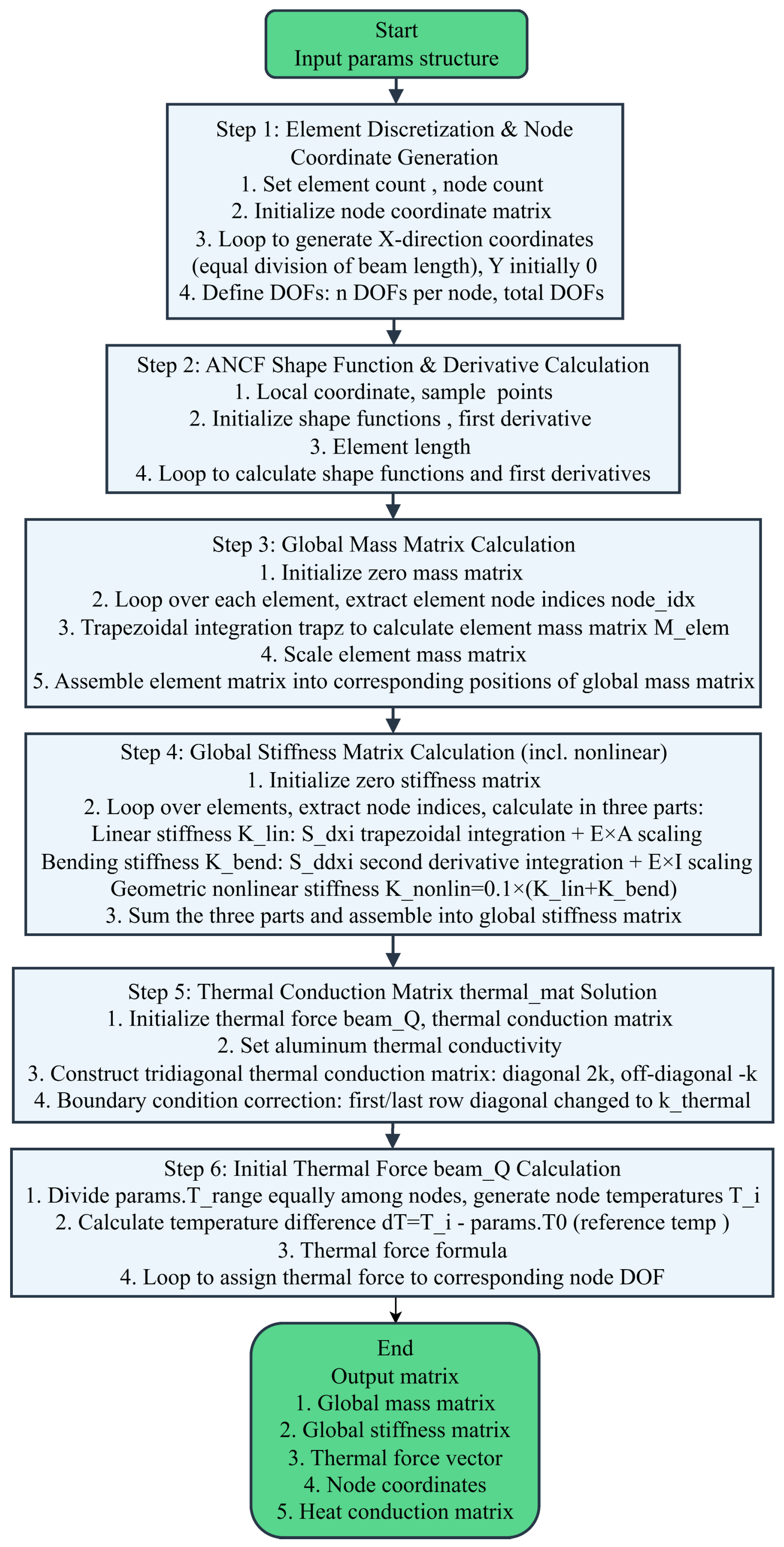
This section establishes the thermo-mechanical coupling dynamic model for variable-geometry deployable antennas with clearance hinges using the Absolute Nodal Coordinate Formulation (ANCF). It progresses from local component modeling to system-level governing equations, incorporating temperature-dependent material behavior and nonlinear clearance contact. Figure 1 presents a schematic flowchart of the ANCF-based thermo-mechanical coupling matrix assembly procedure. The workflow comprises six main steps: (1) element discretization and node coordinate generation; (2) calculation of ANCF shape functions and their derivatives; (3) assembly of the global temperature-dependent mass matrix; (4) assembly of the global stiffness matrix (including linear and geometric nonlinear parts); (5) construction of the thermal conduction matrix; and (6) computation of the initial thermal force vector. The final outputs are the global mass matrix, global stiffness matrix, thermal force vector, node coordinates, and heat conduction matrix.

2.1. ANCF for Flexible Deployable Antenna Components

The ANCF employs global position and gradient vectors to describe flexible body deformation, inherently eliminating geometric nonlinear errors from large rotations/deformations and enabling unified displacement–temperature field discretization without mesh mismatch.

2.1.1. Element Selection and Nodal Coordinates

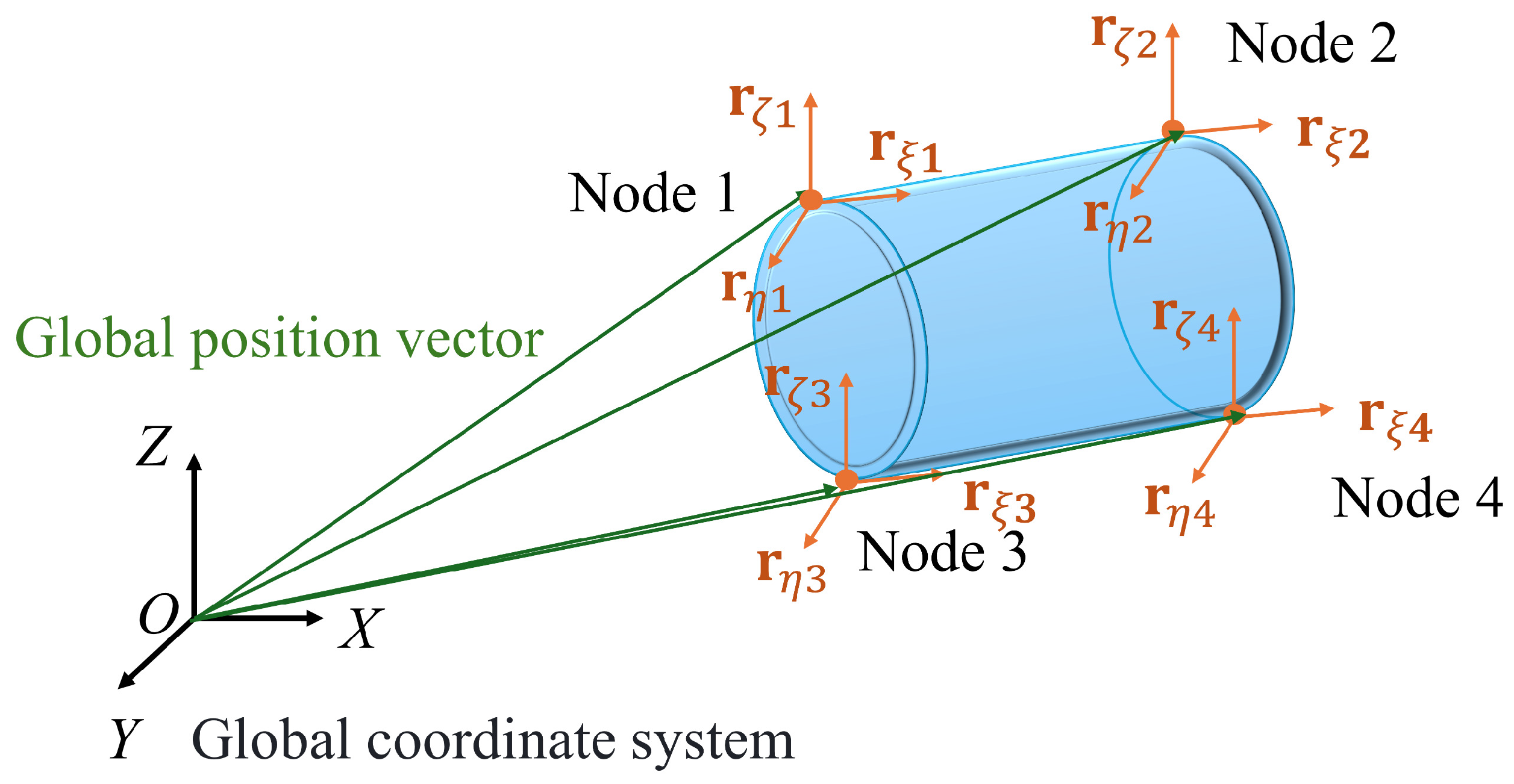
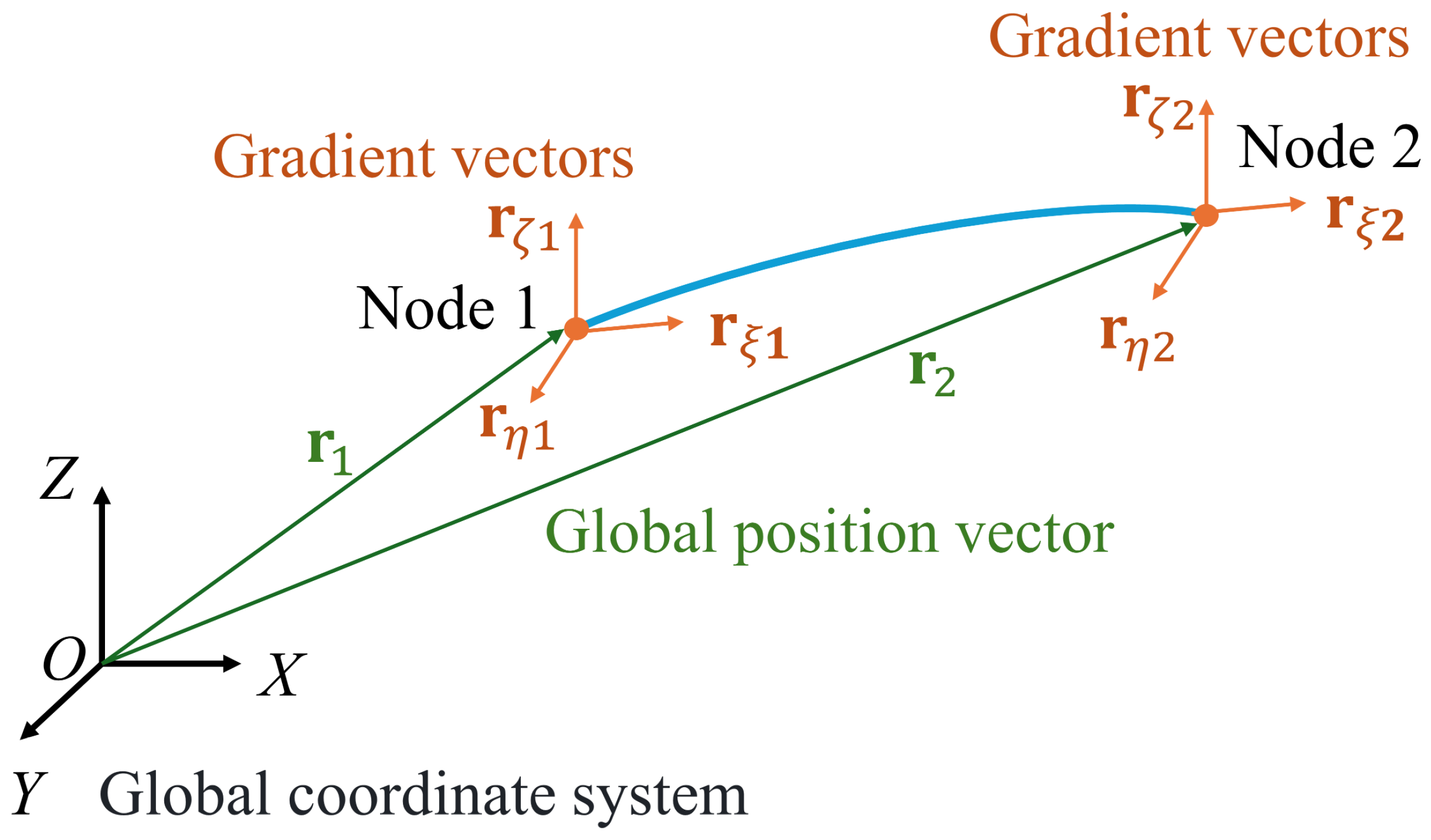
Three fully parameterized ANCF elements are defined uniformly in the global inertial frame. The 4-node 3D thick cylindrical shell element and 2-node 3D thin-walled curved beam element are illustrated in Figure 2 and Figure 3. Unlike the conventional floating frame of reference formulation, the ANCF uses global position and gradient vectors to describe deformation, inherently eliminating geometric nonlinear errors from large rotations and deformations.

3D Thick Cylindrical Shell Element (Manipulator Arms): A 4-node Mindlin–Reissner shell element [36] is adopted to model the main boom and secondary arm, as shown in Figure 2, which accurately captures transverse shear deformation and thickness effects critical for thin-walled cylindrical structures. The nodal coordinates for node i of the shell element are presented below:

$${\mathbf{e}}_i^{\mathrm{shell}}={\left[{\mathbf{r}}_i^T{\mathbf{r}}_{{\xi }_i}^T{\mathbf{r}}_{{\eta }_i}^T{\mathbf{r}}_{{\zeta }_i}^T\right]}^T$$

(1)

where ${\mathbf{r}}_i\in {\mathbb{R}}^3$ is the global position vector of node i, and ${\mathbf{r}}_{{\xi }_i}$, ${\mathbf{r}}_{{\eta }_i}$, ${\mathbf{r}}_{{\zeta }_i}\in {\mathbb{R}}^3$ are the gradient vectors with respect to the local curvilinear coordinates $\xi$ (axial direction along the boom), $\eta$ (circumferential direction), and $\zeta$ (radial direction through the shell thickness), respectively. Each node has 12 degrees of freedom (DOFs).

3D Thin-Walled Curved Beam Element (Truss Reflector): A two-node Timoshenko-based curved beam element [37] is used to model the ring truss reflector, as shown in Figure 3, which avoids the discretization errors introduced by approximating curved truss members with straight beam elements. The nodal coordinates for node i of the beam element are presented below:

$${\mathbf{e}}_i^{\mathrm{beam}}={\left[{\mathbf{r}}_i^T{\mathbf{r}}_{{\xi }_i}^T{\mathbf{r}}_{{\eta }_i}^T{\mathbf{r}}_{{\zeta }_i}^T\right]}^T$$

(2)

where ${\mathbf{r}}_i\in {\mathbb{R}}^3$ is the global position vector of node i, and ${\mathbf{r}}_{{\xi }_i}$, ${\mathbf{r}}_{{\eta }_i}$, ${\mathbf{r}}_{{\zeta }_i}\in {\mathbb{R}}^3$ are the gradient vectors with respect to the local curvilinear coordinates $\xi$ (tangent direction along the beam centerline), $\eta$ and $\zeta$ (two mutually perpendicular transverse directions), respectively. Each node also has 12 DOFs.

Joint Constraints: Key kinematic pairs are formulated via Lagrange multipliers. The spherical joint constraint is $C_s=r_p-r_q=0$. The cylindrical joint adds collinearity constraints, releasing one rotational DOF.

2.1.2. Unified Displacement and Temperature Field Interpolation

Consistent spatial discretization is achieved by using identical shape functions for both the displacement field and the temperature field, thereby eliminating calculation errors caused by mesh mismatch in multi-physics coupling.

The displacement field is interpolated as

$$\mathbf{r}(\xi ,\eta ,\zeta ,t)=\mathbf{S}(\xi ,\eta ,\zeta )\mathbf{e}\left(t\right)$$

(3)

where $\mathbf{S}$ is the shape function matrix and $\mathbf{e}\left(t\right)$ the nodal coordinate vector.

For the 3D beam element, the shape functions are constructed using cubic Hermite polynomials:

$$\mathit{S}=\left[S_1{\mathbf{I}}_3{S}_2{\mathbf{I}}_3{S}_3{\mathbf{I}}_3{S}_4{\mathbf{I}}_3\right]$$

(4)

with

$$S_1=1-3{\xi }^2+2{\xi }^3,S_2=L(\xi -2{\xi }^2+{\xi }^3),S_3=3{\xi }^2-2{\xi }^3,S_4=L(-{\xi }^2+{\xi }^3)$$

where L is the element length, ${\mathbf{I}}_3$ the $3\times 3$ identity matrix, and the products imply Kronecker multiplication.

For the 3D thick shell element, a bicubic polynomial shape function is employed:

$$\mathbf{S}(\xi ,\eta ,\zeta )=S_1\left(\xi \right)S_1\left(\eta \right){\mathbf{I}}_3,\cdots$$

(5)

where $S_1\left(\xi \right)$ and $S_2\left(\eta \right)$ are one-dimensional cubic Hermite polynomials along $\xi$ and $\eta$, respectively, having the same form as above.

The temperature field is interpolated using the same shape functions:

$$T(\xi ,\eta ,\zeta ,t)={\mathbf{S}}_T(\xi ,\eta ,\zeta ){\mathbf{T}}_e\left(t\right)$$

(6)

with ${\mathbf{S}}_T=\mathbf{S}$ and ${\mathbf{T}}_e\left(t\right)$ the element nodal temperature vector. This unified interpolation scheme provides the mathematical foundation for the fully coupled thermo-mechanical governing equations.

2.2. Temperature-Dependent Material Constitutive Model for Extreme Space Thermal Environment

The extreme cyclic temperature fluctuation from −200 °C to 200 °C in the geosynchronous Earth orbit (GEO) will cause significant changes in the physical and mechanical properties of the antenna structural material, aerospace aluminum alloy 6061-T6, which directly affects the mass, stiffness, damping characteristics of the structure and the contact behavior of the clearance hinges. Based on the standard experimental data of aerospace materials, a temperature-dependent constitutive model covering mechanical and thermal physical parameters is established in this section.

The reference temperature is set as $T_0=25 °\mathrm{C}$, and the subscript 0 denotes the parameter value at the reference temperature. The temperature-dependent expressions of each key material parameter are as follows:

• Density:

  $$\rho \left(T\right)={\rho }_0\left[1+{\alpha }_{\rho }(T-T_0)\right]$$
• Young’s modulus (quadratic fit):

  $$E\left(T\right)=E_0\left[1+{\alpha }_E(T-T_0)+{\beta }_E{(T-T_0)}^2\right]$$
• Poisson’s ratio:

  $$\nu \left(T\right)={\nu }_0\left[1+{\alpha }_{\nu }(T-T_0)\right]$$
• Thermal expansion coefficient:

  $${\alpha }_T\left(T\right)={\alpha }_{T0}\left[1+{\alpha }_{{\alpha }_T}(T-T_0)\right]$$
• Thermal conductivity:

  $$k\left(T\right)=k_0\left[1+{\alpha }_k(T-T_0)\right]$$
• Specific heat capacity:

  $$c_p\left(T\right)=c_0\left[1+{\alpha }_c(T-T_0)\right]$$

The reference values and temperature coefficients of each material parameter are listed in

Table 1. Temperature-dependent material parameters of Aluminum Alloy 6061-T6 [44,45].

Parameter	Reference Value	Temperature Coefficient	Applicable Temperature Range
Density ${\rho }_0$	$2700\mathrm{kg}/{\mathrm{m}}^3$	${\alpha }_{\rho }=-2\times {10}^{-5} {°\mathrm{C}}^{-1}$	−200 °C∼200 °C
Young’s Modulus $E_0$	$69\mathrm{GPa}$	${\alpha }_E=-1.5\times {10}^{-4} {°\mathrm{C}}^{-1}$ ${\beta }_E=-5\times {10}^{-7} {°\mathrm{C}}^{-1}$	−200 °C∼200 °C
Poisson’s Ratio ${\nu }_0$	$0.33$	${\alpha }_{\nu }=5\times {10}^{-5} {°\mathrm{C}}^{-1}$	−200 °C∼200 °C
Thermal Expansion Coefficient ${\alpha }_{T0}$	$23.1\times {10}^{-6} {°\mathrm{C}}^{-1}$	${\alpha }_{{\alpha }_T}=1\times {10}^{-4} {°\mathrm{C}}^{-1}$	−200 °C∼200 °C
Thermal Conductivity $k_0$	$167\mathrm{W}/(\mathrm{m}·\mathrm{K})$	${\alpha }_k=0.002 {°\mathrm{C}}^{-1}$	−200 °C∼200 °C
Specific Heat Capacity $c_0$	$896\mathrm{J}/(\mathrm{kg}·\mathrm{K})$	${\alpha }_c=0.001 {°\mathrm{C}}^{-1}$	−200 °C∼200 °C

, covering the full temperature range of the antenna’s on-orbit environment. The model accuracy has been validated by polynomial fitting ($R^2>0.99$) to experimental data for Aluminum Alloy 6061-T6 compiled in the Aerospace Materials Handbook [44] with the applicable environmental range confirmed by NASA space flight thermal specifications [45].

2.3. Theoretical Modeling of Thermo-Structural Coupling with Clearance Nonlinearity

This section establishes a fully coupled framework for the thermally induced vibration of deployable structures, integrating heat transfer, thermal stress, nonlinear contact with friction, and structural dynamics. All fields are discretized via ANCF.

2.3.1. Heat Conduction Governing Equation

Fourier’s law defines the heat flux vector for an isotropic medium as

$$\mathbf{q}=-\lambda \nabla T$$

(7)

where $\lambda$ is thermal conductivity and T is absolute temperature. From energy conservation, the net heat inflow into a volume element $dV=dxdydz$ equals its internal energy change. The three-dimensional transient heat conduction equation is

$$\rho c_p{\displaystyle \frac{\partial T}{\partial t}}=\lambda {\nabla }^{2}T\Rightarrow {\displaystyle \frac{\partial T}{\partial t}}=\alpha {\nabla }^{2}T$$

(8)

where $\rho$ is the density, $c_p$ is the specific heat capacity, and $\alpha =\lambda /\left(\rho c_p\right)$ is the thermal diffusivity. For steady-state conduction $\partial T/\partial t=0$, Equation (8) reduces the Laplace equation ${\nabla }^{2}T=0$. For one-dimensional steady-state conduction with boundary conditions $T\left(x_1\right)=T_1$, $T\left(x_2\right)=T_2$, the temperature distribution and heat transfer rate are

$$T\left(x\right)=T_1+{\displaystyle \frac{T_2-T_1}{x_2-x_1}}(x-x_1),Q=\lambda A{\displaystyle \frac{T_1-T_2}{x_2-x_1}}$$

(9)

with an internal volumetric heat source ${\dot{q}}_v$ (e.g., frictional heating), the governing equation becomes

$$\rho c_p{\displaystyle \frac{\partial T}{\partial t}}=\lambda {\nabla }^{2}T+{\dot{q}}_v$$

(10)

For one-dimensional steady-state conduction with uniform ${\dot{q}}_v$ and boundary conditions $T\left(0\right)=T_0$, ${dT/dx|}_{x=L}=0$, the temperature distribution is

$$T\left(x\right)=T_0+{\displaystyle \frac{{\dot{q}}_v}{\lambda }}\left(Lx-{\displaystyle \frac{x^2}{2}}\right),T_{max}=T_0+{\displaystyle \frac{{\dot{q}}_v{L}^2}{2\lambda }}$$

(11)

2.3.2. Thermal Strain and Thermal Stress Formulation

For a temperature change $\Delta T=T-T_0$, the linear thermal strain is ${\epsilon }_{\mathrm{th},x}={\alpha }_L\Delta T$, where ${\alpha }_L$ is the linear thermal expansion coefficient. For isotropic materials, the three-dimensional thermal strain tensor is

$${\epsilon }_{\mathrm{th},x}={\epsilon }_{\mathrm{th},y}={\epsilon }_{\mathrm{th},z}={\alpha }_L(T-T_0),{\gamma }_{\mathrm{th},xy}={\gamma }_{\mathrm{th},yz}={\gamma }_{\mathrm{th},zx}=0$$

(12)

The total strain decomposes as ${\epsilon }_{ij}={\epsilon }_{\mathrm{mech},ij}+{\epsilon }_{\mathrm{th},ij}$. For fully constrained thermal expansion ${\epsilon }_{ij}=0$, substituting ${\epsilon }_{\mathrm{mech},ij}=-{\epsilon }_{\mathrm{th},ij}$ into Hooke’s law yields the three-dimensional thermal stress:

$${\sigma }_{\mathrm{th},x}={\sigma }_{\mathrm{th},y}={\sigma }_{\mathrm{th},z}=-{\displaystyle \frac{E{\alpha }_L\Delta T}{1-2\mu }}$$

(13)

For a one-dimensional bar fixed at both ends, this simplifies to ${\sigma }_{\mathrm{th}}=-E{\alpha }_L\Delta T$ with thermal force $F_{\mathrm{th}}=-EA{\alpha }_L\Delta T$. For a two-dimensional constrained thin plate, the in-plane thermal stress is ${\sigma }_{\mathrm{th},x}={\sigma }_{\mathrm{th},y}=-{\displaystyle \frac{E{\alpha }_L\Delta T}{1-\mu }}$.

Combining the equilibrium equations (without body forces), geometric equations for small deformations, and Hooke’s law with thermal strain, the stress-displacement relationships incorporating thermal effects are

$${\sigma }_x={\displaystyle \frac{E}{(1+\mu )(1-2\mu )}}\left[(1-\mu ){\displaystyle \frac{\partial u}{\partial x}}+\mu \left({\displaystyle \frac{\partial v}{\partial y}}+{\displaystyle \frac{\partial w}{\partial z}}\right)-(1+\mu ){\alpha }_L(T-T_0)\right]$$

(14)

with analogous expressions for ${\sigma }_y$ and ${\sigma }_z$, and shear stresses ${\tau }_{xy}=G(\partial u/\partial y+\partial v/\partial x)$, etc. Substituting these into the equilibrium equations yields the Navier equations for thermal stress:

$$G{\nabla }^2{u}_i+{\displaystyle \frac{G}{1-2\mu }}{\displaystyle \frac{\partial (\nabla ·\mathbf{u})}{\partial x_i}}-{\displaystyle \frac{E{\alpha }_L}{1-2\mu }}{\displaystyle \frac{\partial T}{\partial x_i}}=0(i=x,y,z)$$

(15)

where $\mathbf{u}={\{u,v,w\}}^T$ is the displacement vector, E is Young’s modulus, $\mu$ is Poisson’s ratio, and $G=E/\left[2\right(1+\mu \left)\right]$ is the shear modulus.

2.3.3. Nonlinear Clearance Behavior Modeling with Contact and Friction

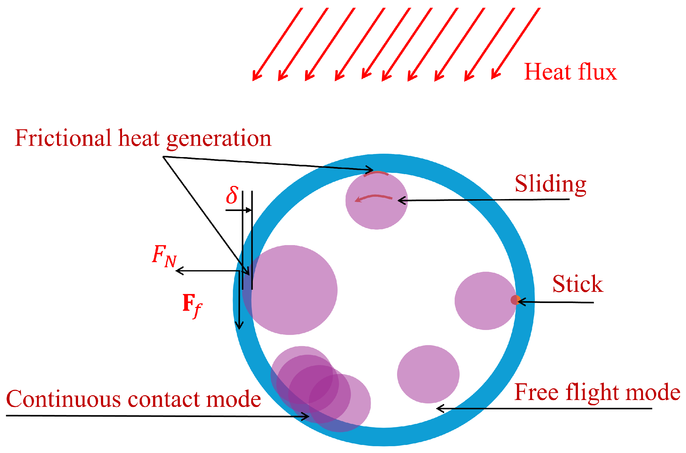
Revolute clearance joints introduce strong nonlinear contact and friction that are bidirectionally coupled with the thermal field through two mechanisms: (1) frictional heat generation at the contact interface, and (2) thermal expansion-induced variation of the radial clearance. A comprehensive schematic of the clearance joint model, showing geometric parameters, contact mechanics, and thermo-mechanical coupling effects, is presented in Figure 4 and Figure 5.

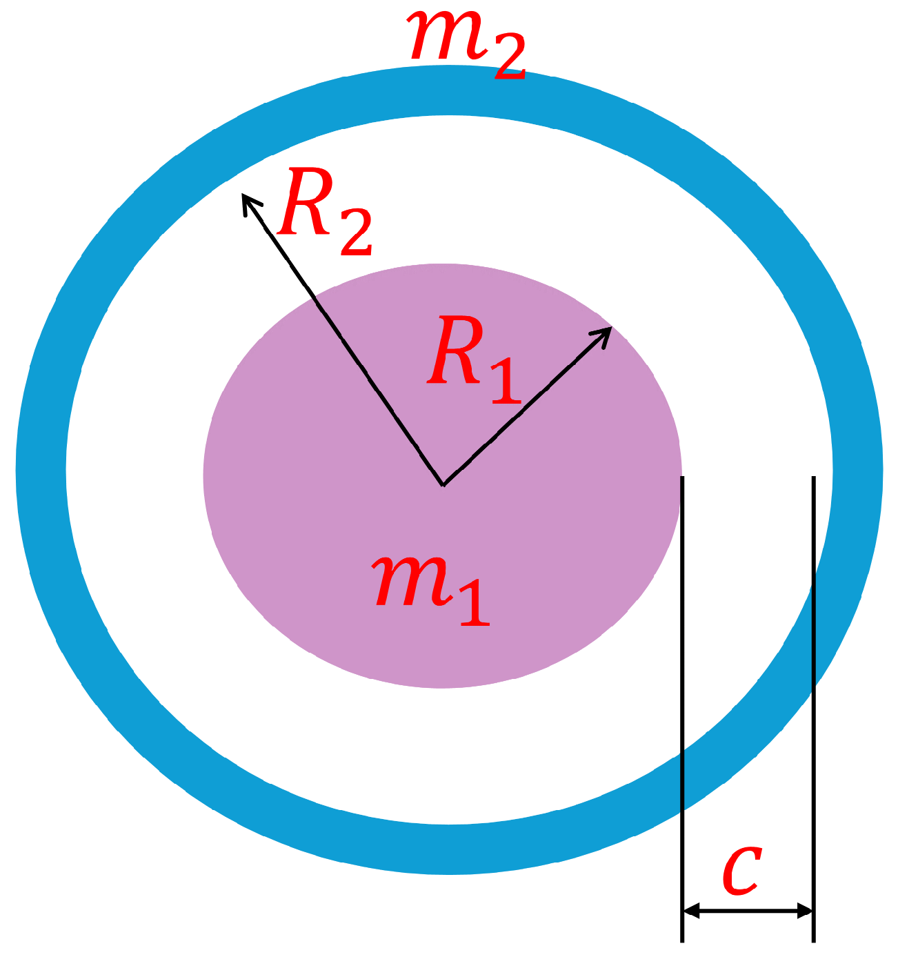
As defined in Figure 4, the radial clearance c is the difference between the bearing inner radius $R_2$ and the journal outer radius $R_1$:

$$c=R_2-R_1$$

(16)

Let $O_b$ and $O_j$ denote the centers of the bearing and journal, respectively, and let $r=\left|{\mathbf{O}}_b{\mathbf{O}}_j\right|$ be the center distance. The penetration depth $\delta$ (positive when contact occurs) is then

$$\delta =r-c$$

(17)

and contact is initiated when $\delta >0$. As illustrated in Figure 5, the clearance joint exhibits four distinct motion regimes: free flight (no contact), continuous contact (permanent contact with varying penetration), sliding (relative tangential motion), and stick (no relative tangential motion).

For two colliding bodies with masses $m_1$ (journal) and $m_2$ (bearing), the normal velocities before and after impact are related by momentum conservation and the coefficient of restitution e, $0\le e\le 1$:

$$v_{1f}={\displaystyle \frac{m_1-e{m}_2}{m_1+m_2}}{v}_{1i}+{\displaystyle \frac{(1+e)m_2}{m_1+m_2}}{v}_{2i},v_{2f}={\displaystyle \frac{(1+e)m_1}{m_1+m_2}}{v}_{1i}+{\displaystyle \frac{m_2-e{m}_1}{m_1+m_2}}{v}_{2i}$$

(18)

The kinetic energy loss during impact is

$$\Delta E_k={\displaystyle \frac{1-e^2}{2}}·{\displaystyle \frac{m_1{m}_2}{m_1+m_2}}{\left(v_{1i}-v_{2i}\right)}^2$$

(19)

For the special case of impact against a rigid fixed stop $m_2\to \infty$, the post-collision velocity simplifies to $v_f=-e{v}_i$, and the average impact force is ${\overline{F}}_{\mathrm{imp}}=m\left|v_i\right|(1+e)/\Delta t$ with $\Delta t$ the collision duration.

The non-instantaneous elastic contact is described by a modified Hertz model that accounts for both elastic deformation and energy dissipation:

$$F_N(T,\delta )=K_c\left(T\right){\delta }^{3/2}\left[1+{\displaystyle \frac{3(1-e^2)}{2e}}·{\displaystyle \frac{\dot{\delta }}{{\dot{\delta }}_0}}\right]H\left(\delta \right)$$

(20)

where $K_c\left(T\right)$ is the temperature-dependent Hertzian contact stiffness, $\dot{\delta }$ is the normal relative velocity, ${\dot{\delta }}_0$ is the reference impact velocity, and $H(·)$ is the Heaviside step function, $H\left(\delta \right)=1$ for $\delta >0$, $H\left(\delta \right)=0$ otherwise. The contact stiffness is given by

$$K_c={\displaystyle \frac{4\sqrt{R}}{3}}{\left({\displaystyle \frac{1-{\nu }_1^2}{E_1}}+{\displaystyle \frac{1-{\nu }_2^2}{E_2}}\right)}^{-1}$$

(21)

in which $R=R_1{R}_2/(R_1+R_2)$ is the equivalent contact radius, $E_1$, $E_2$ are the Young’s moduli, and ${\nu }_1$, ${\nu }_2$ are the Poisson’s ratios of the journal and bearing materials. For perfectly elastic collisions $(e=1)$, the maximum penetration depth, maximum impact force, and collision duration are

$${\delta }_{max}={\left({\displaystyle \frac{15m{v}_i^2}{16K_c}}\right)}^{2/5},F_{\mathrm{imp},max}=K_c^{2/5}{\left({\displaystyle \frac{15m{v}_i^2}{16}}\right)}^{3/5},\Delta t=2.943{\left({\displaystyle \frac{m^2}{K_c^2{v}_i}}\right)}^{1/5}.$$

(22)

The tangential friction force follows a regularized Coulomb friction law to avoid numerical singularity at zero relative velocity:

$$F_f(T,\dot{\xi })=-{\mu }_k\left(T\right)\left|F_N\right|{\displaystyle \frac{\dot{\xi }}{|\dot{\xi }|+ϵ}},ϵ\ll 1$$

(23)

where ${\mu }_k\left(T\right)$ is the temperature-dependent kinetic friction coefficient, $\dot{\xi }$ is the relative tangential velocity at the contact point, and $ϵ$ is a small regularization parameter. The maximum static friction force is bounded by $F_{\mathrm{fs},max}={\mu }_s\left|F_N\right|$ with the static friction coefficient ${\mu }_s>{\mu }_k$.

As shown in Figure 5, frictional sliding generates heat at the contact interface, which acts as a volumetric heat source. The frictional heat generation rate is

$${\dot{Q}}_f\left(T\right)={\mu }_k\left(T\right)|F_N\left|\right|\dot{\xi }|$$

(24)

The generated heat is partitioned between the journal and bearing according to their thermal properties. The heat partition coefficient ${\beta }_i$ for body i is

$${\beta }_i={\displaystyle \frac{\sqrt{{\lambda }_i{\rho }_i{c}_{p,i}}}{\sqrt{{\lambda }_1{\rho }_1{c}_{p,1}}+\sqrt{{\lambda }_2{\rho }_2{c}_{p,2}}}},{\beta }_1+{\beta }_2=1$$

(25)

where ${\lambda }_i$, ${\rho }_i$, and $c_{p,i}$ are the thermal conductivity, density, and specific heat capacity of body i.

The volumetric heat generation rate within the contact layer of thickness ${\delta }_c$ is ${\dot{q}}_{v,f}={\beta }_i{\dot{Q}}_f/\left(A_c{\delta }_c\right)$ with $A_c$ representing the contact area.

A linear temperature-dependent kinetic friction coefficient is adopted:

$${\mu }_k\left(T\right)={\mu }_{k0}\left[1+k_T(T-T_0)\right]$$

(26)

where ${\mu }_{k0}$ is the reference friction coefficient at $T_0=25 °\mathrm{C}$ and $k_T$ is the temperature coefficient. Substituting Equation (21) into Equations (19) and (20) and assuming a pure sliding condition gives the temperature-dependent friction force magnitude and heat generation rate:

$$F_f\left(T\right)={\mu }_{k0}\left[1+k_T(T-T_0)\right]F_N,{\dot{Q}}_f\left(T\right)={\mu }_{k0}\left[1+k_T(T-T_0)\right]|F_N\left|\right|\dot{\xi }|$$

(27)

This establishes a bidirectional thermo-mechanical coupling: temperature changes alter friction properties, which in turn modify the friction force and the frictional heat generation.

2.3.4. Fully Coupled Thermo-Structural Dynamic Governing Equations

Based on the ANCF discretization, the thermo-structural coupling energy functional is first constructed, and the coupled dynamic governing equations are derived via Lagrange’s equation, integrating the temperature-dependent material properties, thermal load, and gap nonlinear forces.

A. 

Energy Functional with Temperature Dependence

The system kinetic energy K, considering the temperature dependence of material density $\rho \left(T\right)$, is expressed as

$$K={\displaystyle \frac{1}{2}}{\int }_V\rho \left(T\right){\dot{u}}^T\dot{u}dV={\displaystyle \frac{1}{2}}{\dot{e}}^T\left({\int }_V\rho \left(T\right)S^{T}SdV\right)\dot{e}={\displaystyle \frac{1}{2}}{\dot{e}}^{T}M\left(T\right)\dot{e}$$

(28)

where $\mathbf{u}=\mathbf{Se}$ is the displacement field discretized by ANCF shape functions $\mathbf{S}$, $\mathbf{e}$ is the nodal coordinate vector, $\dot{\mathbf{e}}$ is the first time derivative of $\mathbf{e}$, and $\mathbf{M}\left(T\right)$ is the temperature-dependent mass matrix. For an ANCF beam element, the mass matrix is

$$\mathbf{M}\left(T\right)={\int }_L\rho \left(T\right)A\left(\xi \right)S{\left(\xi \right)}^{T}S\left(\xi \right)d\xi$$

(29)

with the analytical integration result:

$${\int }_L{\mathbf{S}}^T\mathbf{S}dL={\displaystyle \frac{{\rho }_{0}AL}{420}}\left[\begin{array}{cccc}156& 22L& 54& -13L\\ 22L& 4L^2& 13L& -3L^2\\ 54& 13L& 156& -22L\\ -13L& -3L^2& -22L& 4L^2\end{array}\right]\otimes {\mathbf{I}}_3$$

(30)

where A is the cross-sectional area of the beam, L is the element length, ${\rho }_0$ is the reference density, and ${\mathbf{I}}_3$ is the $3\times 3$ identity matrix.

The system total potential energy consists of elastic potential energy $V_e$ and thermal potential energy $V_T$. The elastic potential energy, considering the temperature dependence of Young’s modulus $E\left(T\right)$, is

$$V_e={\displaystyle \frac{1}{2}}{\int }_V{\mathit{\sigma }}^T{\mathit{\epsilon }}_{e}dV$$

(31)

where the stress $\mathit{\sigma }=\mathbf{C}\left(T\right){\mathit{\epsilon }}_e$, $\mathbf{C}\left(T\right)$ is the temperature-dependent elasticity matrix, and the elastic strain ${\mathit{\epsilon }}_e=\mathit{\epsilon }-{\mathit{\epsilon }}_T$ with $\mathit{\epsilon }$ being the total strain and ${\mathit{\epsilon }}_T$ the thermal strain. For an ANCF beam element, the total strain is

$$\mathit{\epsilon }=\left[\begin{array}{c}{\displaystyle \frac{\partial u}{\partial x}}\\ y{\displaystyle \frac{{\partial }^{2}v}{\partial x^2}}\\ z{\displaystyle \frac{{\partial }^{2}w}{\partial x^2}}\end{array}\right]=\mathbf{B}\left(\xi \right)\mathbf{e}$$

(32)

where the strain-displacement matrix $\mathbf{B}\left(\xi \right)$ is

$$\mathbf{B}\left(\xi \right)=\left[\begin{array}{ccc}{\mathbf{S}}_x^T& 0& 0\\ 0& y{\mathbf{S}}_{xx}^T& 0\\ 0& 0& z{\mathbf{S}}_{xx}^T\end{array}\right]\otimes {\mathbf{I}}_3$$

(33)

with ${\mathbf{S}}_x=\partial \mathbf{S}/\partial x$ and ${\mathbf{S}}_{xx}={\partial }^2\mathbf{S}/\partial x^2$. The thermal strain is

$${\mathit{\epsilon }}_T={\alpha }_T(T-T_0){\mathbf{I}}_3$$

(34)

Substituting $\mathit{\sigma }=\mathbf{C}\left(T\right)(\mathbf{Be}-{\mathit{\epsilon }}_T)$ into Equation (31), the elastic potential energy is expanded as

$$V_e={\displaystyle \frac{1}{2}}{\mathbf{e}}^T{\mathbf{K}}_e\left(T\right)\mathbf{e}-{\mathbf{e}}^T{\mathbf{F}}_T\left(T\right)+V_{T0}$$

(35)

where ${\mathbf{K}}_e\left(T\right)={\int }_V\mathbf{C}\left(T\right){\mathbf{B}}^T\mathbf{B}dV$ is the temperature-dependent elastic stiffness matrix, ${\mathbf{F}}_T\left(T\right)={\int }_V{\mathbf{B}}^T\mathbf{C}\left(T\right){\mathit{\epsilon }}_{T}dV$ is the thermal load vector, and $V_{T0}$ is a constant term that does not affect the dynamic equation. For an ANCF beam element, the thermal load vector is

$${\mathbf{F}}_T\left(T\right)={\int }_{L}E\left(T\right){\alpha }_T\Delta TA\left(\xi \right)\mathbf{B}\left(\xi \right)d\xi$$

(36)

The thermal potential energy, related to the temperature gradient, is

$$V_T={\displaystyle \frac{1}{2}}{\int }_{V}k\left(T\right){(\nabla T)}^{2}dV={\displaystyle \frac{1}{2}}{\mathbf{T}}_e^T{\mathbf{K}}_T\left(T\right){\mathbf{T}}_e$$

(37)

where ${\mathbf{T}}_e$ is the nodal temperature vector, ${\mathbf{K}}_T\left(T\right)={\int }_{V}k\left(T\right){\mathbf{B}}_T^T{\mathbf{B}}_{T}dV$ is the thermal conduction stiffness matrix, and ${\mathbf{B}}_T$ is the temperature gradient–nodal temperature matrix.

The system dissipation energy includes structural damping dissipation energy $D_s$ and thermal damping dissipation energy $D_h$. The structural damping adopts the Rayleigh damping model:

$$D_s={\displaystyle \frac{1}{2}}{\dot{\mathbf{e}}}^T\left({\alpha }_M\mathbf{M}\left(T\right)+{\alpha }_K{\mathbf{K}}_e\left(T\right)\right)\dot{\mathbf{e}}={\displaystyle \frac{1}{2}}{\dot{\mathbf{e}}}^T{\mathbf{C}}_s\left(T\right)\dot{\mathbf{e}}$$

(38)

where ${\alpha }_M$ and ${\alpha }_K$ are Rayleigh damping coefficients, and ${\mathbf{C}}_s\left(T\right)$ is the structural damping matrix. The thermal damping dissipation energy is

$$D_h={\displaystyle \frac{1}{2}}{\int }_V\rho \left(T\right)c_p\left(T\right){\dot{T}}^{2}dV={\displaystyle \frac{1}{2}}{\dot{\mathbf{T}}}_e^T{\mathbf{C}}_h\left(T\right){\dot{\mathbf{T}}}_e$$

(39)

where ${\mathbf{C}}_h\left(T\right)={\int }_V\rho \left(T\right)c_p\left(T\right){\mathbf{S}}_T^T{\mathbf{S}}_{T}dV$ is the thermal damping matrix, and ${\mathbf{S}}_T$ is the temperature shape function matrix.

B. 

Coupled Governing Equations

The discrete heat conduction equation, considering solar radiation heat flux $q_s$ and surface radiation heat dissipation $q_r$, is derived as

$${\mathbf{C}}_h\left(T\right){\dot{\mathbf{T}}}_e+{\mathbf{K}}_T\left(T\right){\mathbf{T}}_e=\mathbf{Q}\left(t\right)$$

(40)

where $\mathbf{Q}\left(t\right)={\int }_A(q_s-q_r)dA$ is the thermal load vector, and A is the heat-receiving surface area.

Based on Lagrange’s equation,

$${\displaystyle \frac{d}{dt}}\left({\displaystyle \frac{\partial K}{\partial \dot{\mathbf{e}}}}\right)-{\displaystyle \frac{\partial K}{\partial \mathbf{e}}}+{\displaystyle \frac{\partial (V_e+V_T)}{\partial \mathbf{e}}}+{\displaystyle \frac{\partial (D_s+D_h)}{\partial \dot{\mathbf{e}}}}={\mathbf{F}}_{\mathrm{ext}}$$

(41)

Neglecting the direct influence of thermal potential energy and thermal damping on the displacement field (weak coupling assumption), the structural dynamic equation is derived as

$$\mathbf{M}\left(T\right)\ddot{\mathbf{e}}+{\mathbf{C}}_s\left(T\right)\dot{\mathbf{e}}+{\mathbf{K}}_e\left(T\right)\mathbf{e}={\mathbf{F}}_T\left(T\right)+{\mathbf{F}}_{\mathrm{ext}}+{\mathbf{F}}_{\mathrm{gap}}$$

(42)

where ${\mathbf{F}}_{\mathrm{ext}}$ is the external load vector (deployment driving force and satellite body inertial force), and ${\mathbf{F}}_{\mathrm{gap}}$ is the clearance hinge force vector. The normal contact force follows a modified Hertz model with hysteresis damping:

$$F_n(T,\delta )=K_c\left(T\right){\delta }^{3/2}\left[1+{\displaystyle \frac{3(1-e^2)}{2e}}·{\displaystyle \frac{\delta }{{\delta }_0}}\right]H(-g),e>0$$

(43)

and the tangential friction obeys Coulomb’s law with a temperature-dependent coefficient $\mu \left(T\right)$ and a regularization parameter $\epsilon$:

$$F_t(T,\dot{\xi })=-\mu \left(T\right)\left|F_n\right|{\displaystyle \frac{\dot{\xi }}{\left|\dot{\xi }\right|+\epsilon }},\epsilon \ll 1$$

(44)

The complete clearance hinge force vector is then $F_{\mathrm{gap}}=\sum (F_{n}n+F_{t}t)$ with $n,t$ the unit normal and tangential vectors.

Finally, the fully coupled thermo-structural dynamic governing equations are established by combining the heat conduction Equation (40) and the structural dynamic Equation (42):

$$\left\{\begin{array}{cc}\hfill M\left(T\right)\ddot{e}+C_s\left(T\right)\dot{e}+K_e\left(T\right)e& =F_T\left(T_e\right)+F_{\mathrm{ext}}+F_{\mathrm{gap}}\hfill \\ \hfill C_h\left(T\right){\dot{T}}_e+K_T\left(T\right)T_e& =Q\left(t\right)\hfill \end{array}\right.$$

(45)

This equation set realizes one-way coupling from the temperature field to the displacement field via the thermal load $F_T\left(T_e\right)$. Two-way coupling can be implemented by including frictional heat generation and gap-variation-induced heat flux changes.

3. Numerical Solution Methodology

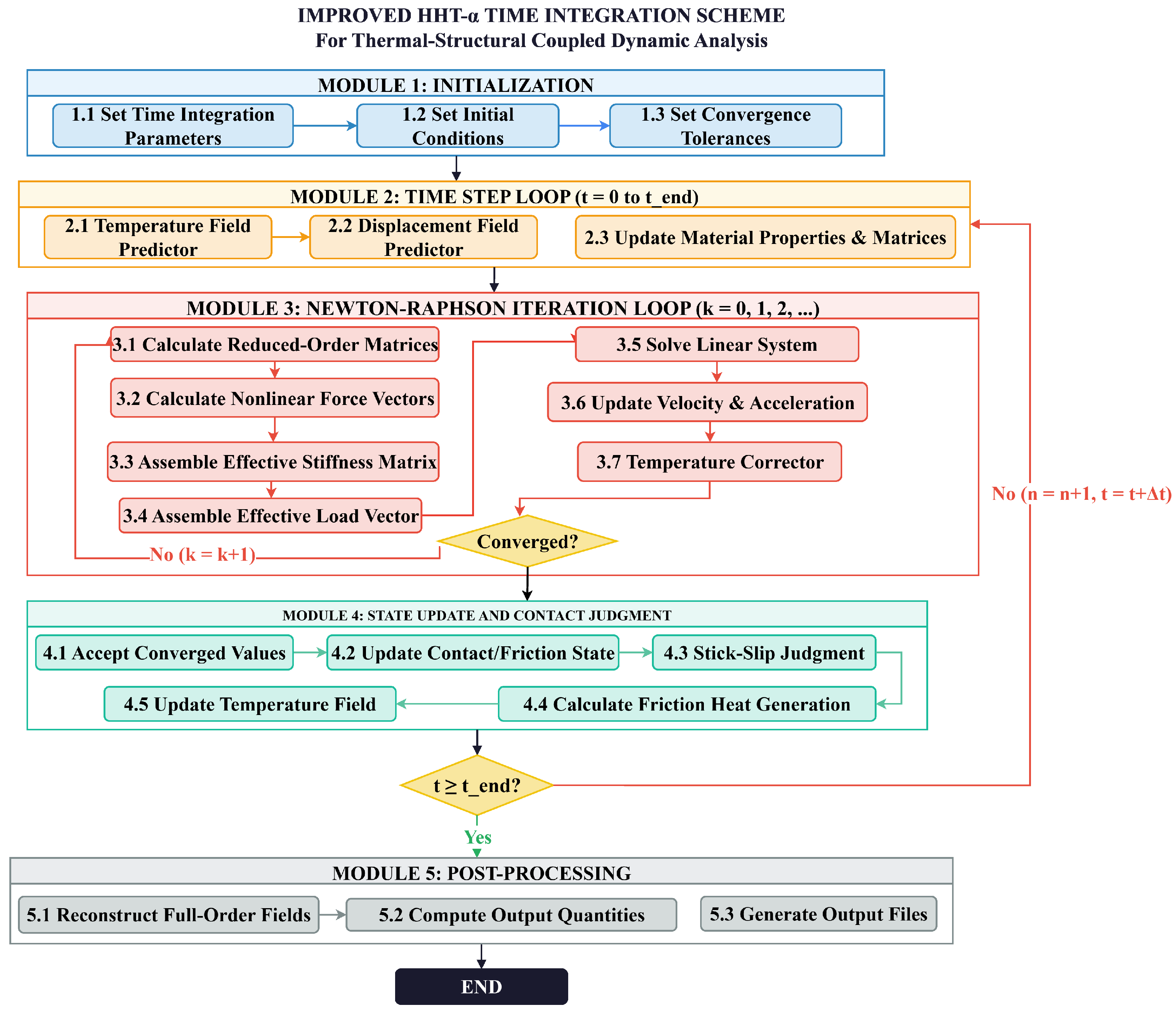
This section presents a robust numerical framework for the thermo-mechanical coupled dynamic system with temperature-dependent frictional contact and clearance effects, as illustrated in the flowchart of Figure 6. The core is an improved HHT-$\alpha$ implicit integration algorithm tailored for strong nonlinearities from time-varying temperature fields, stick–slip friction, and unilateral contact constraints.

3.1. Governing Equations of the Thermo-Mechanical Coupled System

The system is governed by fully coupled differential-algebraic equations (DAEs) comprising structural dynamics and transient heat conduction with two-way coupling via temperature-dependent material properties and frictional heating.

3.1.1. Mechanical Field Dynamic Equilibrium

For a flexible multibody system with n degrees of freedom, the semi-discretized equilibrium equation is established in Section 2.3.4:

$$\mathbf{M}\left(T\right)\ddot{\mathbf{e}}\left(t\right)+{\mathbf{C}}_s\left(T\right)\dot{\mathbf{e}}\left(t\right)+{\mathbf{K}}_e\left(T\right)\mathbf{e}\left(t\right)={\mathbf{F}}_T\left({\mathbf{T}}_e\right)+{\mathbf{F}}_{\mathrm{ext}}\left(t\right)+{\mathbf{F}}_{\mathrm{gap}}(T,\mathbf{e},\dot{\mathbf{e}})$$

(46)

where $\mathbf{M}\left(T\right)$ is the temperature-dependent mass matrix, ${\mathbf{C}}_s\left(T\right)$ is the structural damping matrix (Rayleigh damping), ${\mathbf{K}}_e\left(T\right)$ is the temperature-dependent elastic stiffness matrix, ${\mathbf{F}}_T\left({\mathbf{T}}_e\right)$ is the thermal load vector, ${\mathbf{F}}_{\mathrm{ext}}\left(t\right)$ is the external load vector (deployment driving force and inertial force), and ${\mathbf{F}}_{\mathrm{gap}}(T,\mathbf{e},\dot{\mathbf{e}})$ is the nonlinear clearance hinge force vector encompassing normal contact and tangential friction.

The normal contact force follows the modified Hertz model defined in Section 2.3.4:

$$F_n(T,\delta )=K_c\left(T\right){\delta }^{3/2}\left[1+{\displaystyle \frac{3(1-e^2)}{2e}}·{\displaystyle \frac{\delta }{{\delta }_0}}\right]H(-g),e>0$$

(47)

where $\delta$ is the indentation depth, $K_c\left(T\right)$ is the temperature-dependent Hertzian contact stiffness, $\dot{\delta }$ is the normal relative velocity, ${\dot{\delta }}_0$ is a reference impact velocity, g is the gap function (negative when in contact), and $H(·)$ is the Heaviside step function.

Tangential friction follows Coulomb’s law with a temperature-dependent coefficient $\mu \left(T\right)$:

$$F_t(T,\dot{\xi })=-\mu \left(T\right)\left|F_n\right|{\displaystyle \frac{\dot{\xi }}{\left|\dot{\xi }\right|+\epsilon }},\epsilon \ll 1$$

(48)

where $\dot{\xi }$ is the relative tangential velocity.

3.1.2. Temperature Field Transient Heat Conduction

The 3D transient heat conduction equation with frictional heat source is

$$\rho \left(T\right)c_p\left(T\right){\displaystyle \frac{\partial T}{\partial t}}=\nabla ·\left(k\left(T\right)\nabla T\right)+q_v(\dot{\mathbf{u}},T)$$

(49)

where $q_v(\dot{\mathbf{u}},T)={\displaystyle \frac{1}{V_c}}{\mathbf{t}}_t\left(T\right)·{\dot{\mathbf{u}}}_t{A}_c\left(T\right)$ is volumetric frictional heat generation. After discretization,

$${\mathbf{C}}_h\left(T\right)\dot{\mathbf{T}}\left(t\right)+{\mathbf{K}}_T\left(T\right)\mathbf{T}\left(t\right)={\mathbf{Q}}_c(T,\dot{\mathbf{u}})+{\mathbf{Q}}_e\left(t\right)$$

(50)

3.1.3. Numerical and Physical Parameters

All numerical and physical parameters used in the simulations are summarized in

Table 2. Summary of numerical and physical parameters used in all simulations.

Parameter Category	Parameter	Symbol	Value	Determination Method
Improved HHT-$\alpha$ algorithm	Numerical damping coefficient	$\alpha$	$-0.10$	Optimized for second-order accuracy and high-frequency dissipation
	Newmark displacement coefficient	$\beta$	$0.3025$	$\beta ={(1-\alpha )}^2/4$
	Newmark velocity coefficient	$\gamma$	$0.60$	$\gamma =(1-2\alpha )/2$
	Spectral radius at ∞	${\rho }_{\infty }$	$0.818$	${\rho }_{\infty }=(1+\alpha )/(1-\alpha )$
Newton–Raphson iteration	Force residual tolerance	${\epsilon }_F$	$1\times {10}^{-6}\mathrm{N}$	Numerical convergence test
	Displacement increment tolerance	${\epsilon }_u$	$1\times {10}^{-9}\mathrm{m}$	Numerical convergence test
	Maximum iterations per step	$N_{max}$	25	Numerical stability test
Adaptive time stepping	Initial time step	$\Delta t_0$	$1\times {10}^{-4}\mathrm{s}$	Convergence verification
	Minimum time step	$\Delta t_{min}$	$1\times {10}^{-7}\mathrm{s}$	Stability requirement
	Maximum time step	$\Delta t_{max}$	$5\times {10}^{-4}\mathrm{s}$	Efficiency consideration
	Increase factor	$f_{\mathrm{inc}}$	$1.2$	Convergence-rate-based optimization
	Decrease factor	$f_{\mathrm{dec}}$	$0.5$	Convergence-rate-based optimization
Contact mechanics	Coefficient of restitution	e	$0.85$	Experimental impact test, Al6061-T6 [34,39]
	Reference impact velocity	${\delta }_0$	$0.1\mathrm{m}/\mathrm{s}$	Aerospace standard [34]
	Tangential regularization	$\epsilon$	$1\times {10}^{-4}\mathrm{m}/\mathrm{s}$	Singularity avoidance
Structural damping	Mass proportional coefficient	${\alpha }_M$	$0.12{\mathrm{s}}^{-1}$	Modal analysis, 0.5% damping, modes 1–2
	Stiffness proportional coefficient	${\alpha }_K$	$1.5\times {10}^{-4}\mathrm{s}$	Modal analysis, 0.5% damping, modes 1–2

. The improved HHT-$\alpha$ algorithm coefficients $\alpha ,\beta ,\gamma$ provide second-order accuracy, unconditional stability, and a high-frequency spectral radius ${\rho }_{\infty }=0.818$, which effectively damps spurious contact oscillations while preserving low-frequency dynamics.

A staggered adaptive time-stepping strategy automatically adjusts the step size based on the Newton–Raphson convergence rate, reducing computational cost during smooth motion phases and maintaining accuracy during contact-impact events. The thermal and mechanical time steps are synchronized to ensure consistent two-way coupling.

Contact parameters are taken from experimental data for Al 6061-T6 and aerospace standards. Rayleigh damping coefficients are calibrated to match the measured $0.5\%$ damping ratio of aluminium truss structures, yielding realistic energy dissipation.

3.2. Improved HHT-$\alpha$ Implicit Integration Algorithm

The HHT-$\alpha$ method extends Newmark-$\beta$ with controllable numerical damping, maintaining second-order accuracy and unconditional stability. The improved formulation incorporates real-time temperature-dependent matrix updates, embedded stick–slip contact judgment, and consistent linearization.

3.2.1. Standard HHT-$\alpha$ Formulation

The modified equilibrium equation is

$$\mathbf{M}{\ddot{\mathbf{u}}}_{n+1}+(1+\alpha )(\mathbf{C}{\dot{\mathbf{u}}}_{n+1}+{\mathbf{Ku}}_{n+1}-{\mathbf{F}}_{n+1})-\alpha (\mathbf{C}{\dot{\mathbf{u}}}_n+{\mathbf{Ku}}_n-{\mathbf{F}}_n)=0$$

(51)

The Newmark update formulas are

$${\mathbf{u}}_{n+1}={\mathbf{u}}_n+\Delta t{\dot{\mathbf{u}}}_n+{\displaystyle \frac{\Delta t^2}{2}}[(1-2\beta ){\ddot{\mathbf{u}}}_n+2\beta {\ddot{\mathbf{u}}}_{n+1}]$$

(52)

$${\dot{\mathbf{u}}}_{n+1}={\dot{\mathbf{u}}}_n+\Delta t[(1-\gamma ){\ddot{\mathbf{u}}}_n+\gamma {\ddot{\mathbf{u}}}_{n+1}]$$

(53)

The parameters for second-order accuracy are $\beta ={(1-\alpha )}^2/4$, $\gamma =(1-2\alpha )/2$ with $\alpha \in [-1/3,0]$.

3.2.2. Improved Formulation for Nonlinear Coupled System

With temperature-dependent matrices and contact forces updated at each step, the nonlinear HHT-$\alpha$ equilibrium is

$$\begin{array}{cc}\hfill & {\mathbf{M}}_{n+1}{\ddot{\mathbf{u}}}_{n+1}+(1+\alpha )({\mathbf{C}}_{n+1}{\dot{\mathbf{u}}}_{n+1}+{\mathbf{K}}_{n+1}{\mathbf{u}}_{n+1}-{\mathbf{F}}_{n+1}^e-{\mathbf{F}}_{n+1}^c)-\cdots \hfill \\ \hfill & \cdots -\alpha ({\mathbf{C}}_n{\dot{\mathbf{u}}}_n+{\mathbf{K}}_n{\mathbf{u}}_n-{\mathbf{F}}_n^e-{\mathbf{F}}_n^c)=0\hfill \end{array}$$

(54)

Substituting Newmark relations yields a nonlinear algebraic equation $\mathbf{R}\left({\mathbf{u}}_{n+1}\right)=0$ with residual

$$\begin{array}{cc}\hfill \mathbf{R}\left({\mathbf{u}}_{n+1}\right)& ={\displaystyle \frac{1}{\beta \Delta t^2}}{\mathbf{M}}_{n+1}({\mathbf{u}}_{n+1}-{\widehat{\mathbf{u}}}_n)+(1+\alpha ){\mathbf{K}}_{n+1}{\mathbf{u}}_{n+1}+{\displaystyle \frac{(1+\alpha )\gamma }{\beta \Delta t}}{\mathbf{C}}_{n+1}({\mathbf{u}}_{n+1}-{\tilde{\mathbf{u}}}_n)-\cdots \hfill \\ \hfill & \cdots -(1+\alpha )({\mathbf{F}}_{n+1}^e+{\mathbf{F}}_{n+1}^c)-\alpha ({\mathbf{F}}_n^e+{\mathbf{F}}_n^c-{\mathbf{C}}_n{\dot{\mathbf{u}}}_n-{\mathbf{K}}_n{\mathbf{u}}_n)\hfill \end{array}$$

(55)

3.2.3. Newton–Raphson Iteration

The consistent tangent stiffness matrix is

$${\mathbf{K}}_T={\displaystyle \frac{\partial \mathbf{R}}{\partial {\mathbf{u}}_{n+1}}}={\displaystyle \frac{1}{\beta \Delta t^2}}{\mathbf{M}}_{n+1}+{\displaystyle \frac{(1+\alpha )\gamma }{\beta \Delta t}}{\mathbf{C}}_{n+1}+(1+\alpha ){\mathbf{K}}_{n+1}+(1+\alpha ){\mathbf{K}}_{contact}$$

(56)

where ${\mathbf{K}}_{contact}=-\partial {\mathbf{F}}_{n+1}^c/\partial {\mathbf{u}}_{n+1}$. Iteration proceeds with ${\mathbf{K}}_{contact}=-\partial {\mathbf{F}}_{n+1}^c/\partial {\mathbf{u}}_{n+1}$ until $\Vert \mathbf{R}\Vert /\Vert {\mathbf{F}}_{n+1}^e+{\mathbf{F}}_{n+1}^c\Vert <{ϵ}_{tol}$.

3.2.4. Simultaneous Treatment of Bilateral Constraints and Unilateral Contact in the HHT-$\alpha$ Framework

The improved HHT-$\alpha$ algorithm simultaneously handles bilateral holonomic constraints (Lagrange multipliers with Baumgarte stabilization) and unilateral contact constraints (penalty method) within a unified Newton–Raphson iteration. To ensure robust convergence, the contact forces are fully linearized with respect to both displacement and velocity, and the resulting tangent stiffness and damping matrices are incorporated into the effective stiffness matrix. This guarantees a consistent implicit treatment of all constraints.

For kinematic pairs such as revolute, prismatic, and spherical joints, the constraint equations are expressed as

$$\mathbf{\Phi }(\mathbf{e},t)=\mathbf{0}.$$

(57)

The acceleration-level constraint is

$${\mathbf{\Phi }}_{\mathbf{e}}\ddot{\mathbf{e}}=-{\dot{\mathbf{\Phi }}}_{\mathbf{e}}\dot{\mathbf{e}}-2{\mathbf{\Phi }}_{\mathbf{e}t}\dot{\mathbf{e}}-{\mathbf{\Phi }}_{tt}.$$

(58)

and Baumgarte stabilization is applied to suppress drift:

$${\mathbf{\Phi }}_{\mathbf{e}}\ddot{\mathbf{e}}=-{\dot{\mathbf{\Phi }}}_{\mathbf{e}}\dot{\mathbf{e}}-2{\mathbf{\Phi }}_{\mathbf{e}t}\dot{\mathbf{e}}-{\mathbf{\Phi }}_{tt}-2{\alpha }_B\dot{\mathbf{\Phi }}-{\beta }_B^2\mathbf{\Phi }.$$

(59)

with ${\alpha }_B={\beta }_B=2/\Delta t$ providing a critical damping of constraint violations.

For clearance joints, the gap function $g\left(\mathbf{e}\right)$ defines contact: contact occurs when $g<0$ with penetration $\delta =-g$. The normal contact force is given by the modified Hertz model (Equation (22)) and the tangential friction force by the regularized Coulomb law (Equation (40)). The total contact force on a node pair is

$${\mathbf{F}}_{\mathrm{contact}}=F_N\mathbf{n}+{\mathbf{F}}_f$$

(60)

where $F_N$ depends on $\delta$ and $\dot{\delta }$, and ${\mathbf{F}}_f$ depends on $F_N$ and the relative tangential velocity $\dot{\xi }$. To achieve quadratic convergence of the Newton–Raphson loop, the contact force vector is analytically linearized. The resulting tangent stiffness and damping contributions

$${\mathbf{K}}_{\mathrm{contact}}={\displaystyle \frac{\partial {\mathbf{F}}_{\mathrm{contact}}}{\partial \mathbf{e}}},{\mathbf{C}}_{\mathrm{contact}}={\displaystyle \frac{\partial {\mathbf{F}}_{\mathrm{contact}}}{\partial \dot{\mathbf{e}}}}$$

(61)

are computed at each iteration and added to the effective stiffness matrix.

To achieve a unified implicit treatment of bilateral holonomic constraints and unilateral contact conditions within a thermo-mechanical coupling framework for multibody systems, the improved constraint-solving strategy and nonlinear contact treatment are fully integrated into the HHT-$\alpha$ time integration scheme. This yields a dynamic iterative solution framework with strong numerical stability and computational accuracy. The coupled algorithm simultaneously accounts for the time-varying thermal effects, structural dynamics, kinematic joint constraints, and strongly nonlinear characteristics of clearance contact and friction. Multi-physics and multi-constraint coupling is realized through a staggered solution and iterative correction procedure. The overall HHT-$\alpha$ iteration consists of four core stages: the predictor step, thermal field update, Newton–Raphson iteration for the mechanical field, and post-iteration variable update. The detailed implementation is given below.

• Predictor step
  Predicted displacement, velocity, and acceleration are obtained from the Newmark formulas.
• Thermal field update
  The temperature field $T_{n+1}$ is solved in a staggered manner, and the temperature-dependent material properties and system matrices $\mathbf{M}$, $\mathbf{C}$, $\mathbf{K}$ are then updated.
• Newton–Raphson iteration for the mechanical field
  At each iteration k:
  Evaluate bilateral constraint residuals $\mathbf{\Phi }$ and their Jacobian ${\mathbf{\Phi }}_{\mathbf{e}}$;
  For each clearance joint, compute the gap function; if $g<0$, calculate the contact force ${\mathbf{F}}_{\mathrm{contact}}^{\left(k\right)}$ and its tangent matrices ${\mathbf{K}}_{\mathrm{contact}}$, ${\mathbf{C}}_{\mathrm{contact}}$;
  Assemble the effective stiffness matrix including structural, inertia, and contact contributions:

  $${\mathbf{K}}_{\mathrm{eff}}={\displaystyle \frac{1}{\beta \Delta t^2}}\mathbf{M}+{\displaystyle \frac{(1+\alpha )\gamma }{\beta \Delta t}}\mathbf{C}+(1+\alpha )\mathbf{K}+{\mathbf{K}}_{\mathrm{contact}}+{\displaystyle \frac{(1+\alpha )\gamma }{\beta \Delta t}}{\mathbf{C}}_{\mathrm{contact}}$$

  (62)
  Assemble the mechanical residual including bilateral and contact forces;
  Form the augmented system

  $$\left[\begin{array}{cc}{\mathbf{K}}_{\mathrm{eff}}& {\mathbf{\Phi }}_{\mathbf{e}}^T\\ {\mathbf{\Phi }}_{\mathbf{e}}& \mathbf{0}\end{array}\right]\left[\begin{array}{c}\Delta \mathbf{e}\\ \Delta \mathbf{\lambda }\end{array}\right]=\left[\begin{array}{c}{\mathbf{R}}_{\mathrm{mech}}\\ {\mathbf{R}}_{\mathrm{constraint}}\end{array}\right]$$

  (63)

  and solve for the increments;
  Update $\mathbf{e}$, $\dot{\mathbf{e}}$, $\ddot{\mathbf{e}}$;
  Check convergence using both the force residual and the constraint violation norms. If not converged, reduce the time step and restart.
• Post-iteration updates
  Lagrange multipliers are updated for the next step; frictional heat generation ${\dot{Q}}_f$ is computed and passed to the thermal solver for the subsequent coupling step.

3.3. Sequential Coupling Solution Framework

A staggered strategy solves thermal and mechanical fields sequentially:

• Initialization: Set ${\mathbf{u}}_0,{\dot{\mathbf{u}}}_0,{\ddot{\mathbf{u}}}_0$, ${\mathbf{T}}_0=T_{ref}$, and $\Delta t=min(\Delta t_{mech},\Delta t_{therm})$.
• Temperature Field: Solve $\Delta t=min(\Delta t_{mech},\Delta t_{therm})$.
• Parameter Update: Update $E\left(T\right)$, $G\left(T\right)$, $\mu \left(T\right)$, $K_c\left(T\right)$, and assemble ${\mathbf{M}}_{n+1}$, ${\mathbf{C}}_{n+1}$, ${\mathbf{K}}_{n+1}$.
• Mechanical Field: Solve nonlinear HHT-$\alpha$ system (Section 3.2.3) for ${\mathbf{u}}_{n+1},{\dot{\mathbf{u}}}_{n+1},{\ddot{\mathbf{u}}}_{n+1}$.
• Frictional Heat Update: Compute ${\mathbf{Q}}_c(T_{n+1},{\dot{\mathbf{u}}}_{n+1})$ for the next thermal step.
• Termination Check: If $t_{n+1}\ge t_{max}$, stop; else $n\leftarrow n+1$, return to Step 2.

3.4. Constraint Stabilization

Baumgarte stabilization suppresses constraint drift for holonomic constraints $\Phi (u,t)=0$:

$${\mathbf{\Phi }}_u\ddot{\mathbf{u}}=-{\dot{\mathbf{\Phi }}}_u\dot{\mathbf{u}}-2{\mathbf{\Phi }}_{ut}\dot{\mathbf{u}}-{\mathbf{\Phi }}_{tt}-2{\alpha }_B\dot{\mathbf{\Phi }}-{\beta }_B^2\mathbf{\Phi }$$

(64)

with ${\alpha }_B={\beta }_B=2/\Delta t$. Unilateral contact constraints $g\left(\mathbf{u}\right)\ge 0$ are enforced via the stabilized penalty method.

3.5. Stability and Convergence

Linear stability. For $\alpha \in [-1/3,0]$, the time integration algorithm is unconditionally stable, and the spectral radius at high frequencies is ${\rho }_{\infty }=\left|\alpha \right|$. The typical choice $\alpha =-0.1$ gives ${\rho }_{\infty }=0.1$, which effectively suppresses spurious high-frequency contact oscillations while preserving low-frequency accuracy.

Convergence. Second-order accuracy $O(\Delta t^2)$ is maintained throughout the simulation. Iterative convergence at each time step is enforced by requiring the relative residual to fall below the prescribed tolerance ${ϵ}_{\mathrm{tol}}$. To determine an adequate spatial discretization, a systematic mesh convergence study was performed using four progressively refined meshes with the element length halved at each step (

Table 3. Mesh levels and convergence of key response metrics.

Mesh Level	Element Length (m)	Elements	DOFs	Deployment Time Error (%)	Contact Force Error (%)	Pointing Error (%)	Computing Time (h)
1 (coarse)	0.40	324	4320	8.72	15.34	11.26	1.2
2	0.20	648	8640	3.15	6.89	4.72	3.5
3 (selected)	0.10	1296	17,280	0.87	1.92	1.68	12.8
4 (fine)	0.05	2592	34,560	— (reference)	—	—	52.3

). The total deployment time, the maximum normal contact force at the most heavily loaded hinge, and the final antenna pointing accuracy were taken as the critical response metrics; the finest mesh (Level 4) served as the reference solution.

A convergence criterion of $2\%$ relative error was adopted for all metrics. As shown in Table 3, the Level 3 mesh (element length 0.10 m, 1296 elements, 17,280 degrees of freedom) satisfies this criterion with a maximum error of $1.92\%$. Further refining to the Level 4 mesh eliminates the remaining discretization error, but the marginal improvement (approximately $1.9$ percentage points) comes at the cost of an approximately fourfold increase in computing time. Hence, the Level 3 mesh was selected for all subsequent simulations as the optimal balance between accuracy and efficiency. Energy conservation is verified within $1\%$ relative error, and the monotonic decrease of all response errors with mesh refinement confirms the reliability of the adopted discretization.

4. Numerical Results and Validation

In this section, the accuracy and reliability of the proposed unified dynamic model are first verified through four benchmark validation cases: degeneration validation, pure thermal effect validation, pure clearance effect validation, and full model validation. Subsequently, the dynamic response under three typical deployment configurations is analyzed, and single-factor parametric sensitivity analysis is conducted to quantitatively reveal the influence of temperature, clearance size, and friction coefficient on deployment dynamics. The reference parameters for the three configurations are set according to engineering practice for a GEO large mesh antenna, as listed in

Table 4. Reference parameters of the three typical deployment configurations.

Parameter	Configuration 1: Secondary Arm Extension	Configuration 2: Secondary Arm Rotation	Configuration 3: Reflector Deployment
Structure Type	Main boom + secondary arm (beam elements)	Secondary arm (beam elements)	Ring truss reflector (beam elements)
Characteristic Dimension	Main boom: $65.5\mathrm{m}$; secondary arm: $63.5\mathrm{m}$	Secondary arm: $63.5\mathrm{m}$	Reflector diameter: $100\mathrm{m}$
Deployment Motion	Constant-speed translation: $0.1\mathrm{m}/\mathrm{s}$	Constant-speed rotation: $0.05\mathrm{rad}/\mathrm{s}$	Combined rotation + translation; angular acceleration: $0.01\mathrm{rad}/{\mathrm{s}}^2$
Temperature Condition	Transient: −100 °C → 50 °C at 15 °C/s	Axial temperature gradient: 50 °C/m	Transient: 200 °C → −50 °C at 25 °C/s
Radial Clearance Size	$0.1\mathrm{mm}$	$0.05\mathrm{mm}$	$0.03\mathrm{mm}$
Clearance Hinge Type	Translational joint	Revolute hinge	Revolute hinges + translational joints
Total Deployment Time	$720\mathrm{s}$	$567\mathrm{s}$	$6000\mathrm{s}$

.

4.1. Model Validation

To comprehensively verify the accuracy and reliability of the proposed ANCF-based thermo-mechanical coupling framework, a four-level hierarchical validation strategy was implemented. The model predictions were systematically compared against classical theoretical solutions, published experimental data from the literature, a high-fidelity finite element benchmark constructed in Abaqus 2025, and an internal mesh convergence study. In the first level, the contact force model and thermal expansion coupling were validated against the Hertzian analytical solution and the classical thermo-elastic solution for a single clearance joint, yielding relative errors below $1.5\%$. The second level used published experimental measurements of a deployable truss under thermal cycling, where the predicted tip displacement and joint contact force agreed with the reported data within $3.2\%$. The third level consisted of a direct comparison with an Abaqus 2025 model that employed identical geometry, material properties, and boundary conditions but was discretized with 86,400 C3D8T thermally coupled brick elements; the maximum deviations in deployment time, peak contact force, and final pointing accuracy were all below $2.5\%$, confirming that the ANCF model achieves comparable accuracy at a fraction of the computational cost. The fourth level, an internal mesh convergence analysis, demonstrated that the chosen discretization—1296 ANCF beam elements (1152 truss elements and 144 hinge connection elements) yielding 17,280 degrees of freedom—is sufficient, as doubling the element density altered the key output parameters by less than $1.2\%$. A summary of these validation results is provided in

Table 5. Summary of hierarchical validation for the proposed ANCF thermo-mechanical model.

Validation Level	Reference/Method	Key Metrics	Deviation
I. Theoretical	Hertz contact; classical thermo-elastic solution	Contact force; thermal expansion	<1.5%
II. Experimental	Published deployable truss thermal cycling data	Tip displacement; joint contact force	<3.2%
III. High-fidelity FEM	Abaqus 2025, 86,400 C3D8T elements	Deployment time; max. contact force; pointing accuracy	<2.5%
IV. Mesh convergence	ANCF mesh refinement, 2592 elements vs. 1296	Variation in key outputs	<1.2%

. All simulations were performed on an AMD Ryzen 9 9950X workstation (16 cores, 4.3 GHz, 64 GB RAM) using MATLAB R2025a with performance-critical modules accelerated by C++ MEX, and each 10-second deployment simulation required approximately $12.8$ wall-clock hours with a time step of $1\times {10}^{-4}\mathrm{s}$. The complete software environment and timing breakdown are documented in Section 4.1 to ensure full reproducibility.

4.1.1. Degeneration Validation No Temperature Effect No Clearance

This degeneration validation is performed to verify the fundamental accuracy of the proposed ANCF-based modeling framework under ideal conditions, where temperature-dependent material effects and joint clearance nonlinearity are completely eliminated, degenerating the fully coupled model into a standard flexible multibody dynamic model for the deployable mechanism.

Figure 7 shows the translational, rotational coupling, and pulley–rope pairs that constitute the core motion units of the three deployment configurations. Constraint equations are defined in the global inertial frame for consistency with the ANCF formulation, avoiding cumulative transformation errors.

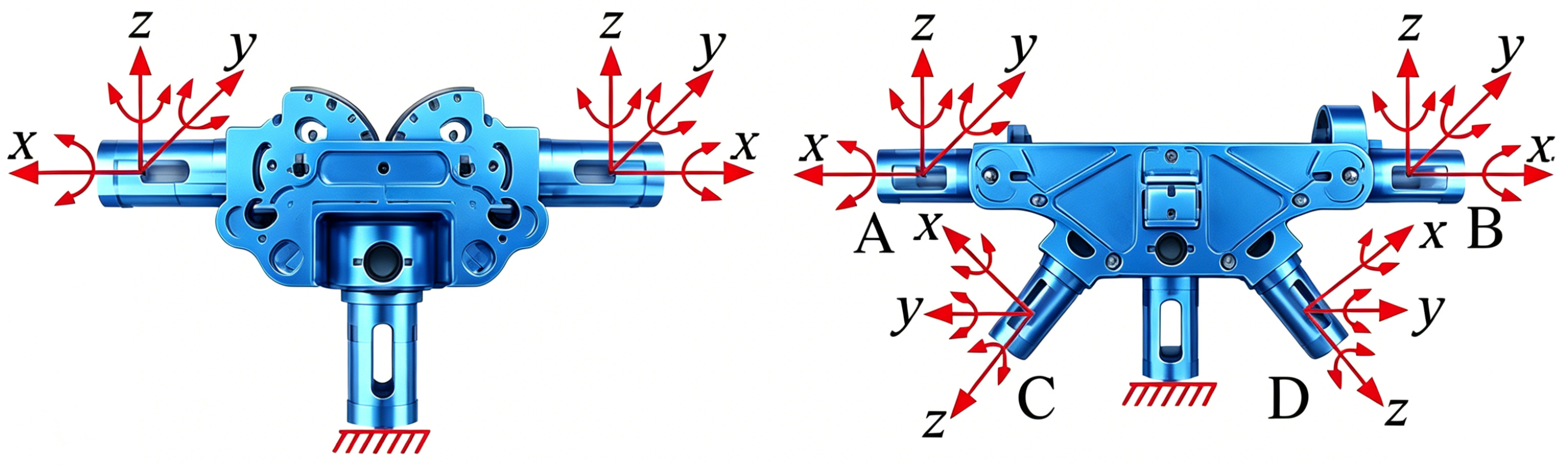
Figure 8 shows the 3D geometry of the deployment joint with global coordinates assigned at branches for DOF characterization and fixed bottom constraints matching ground test conditions. This serves as the geometric basis for ANCF discretization and dynamic response calculation.

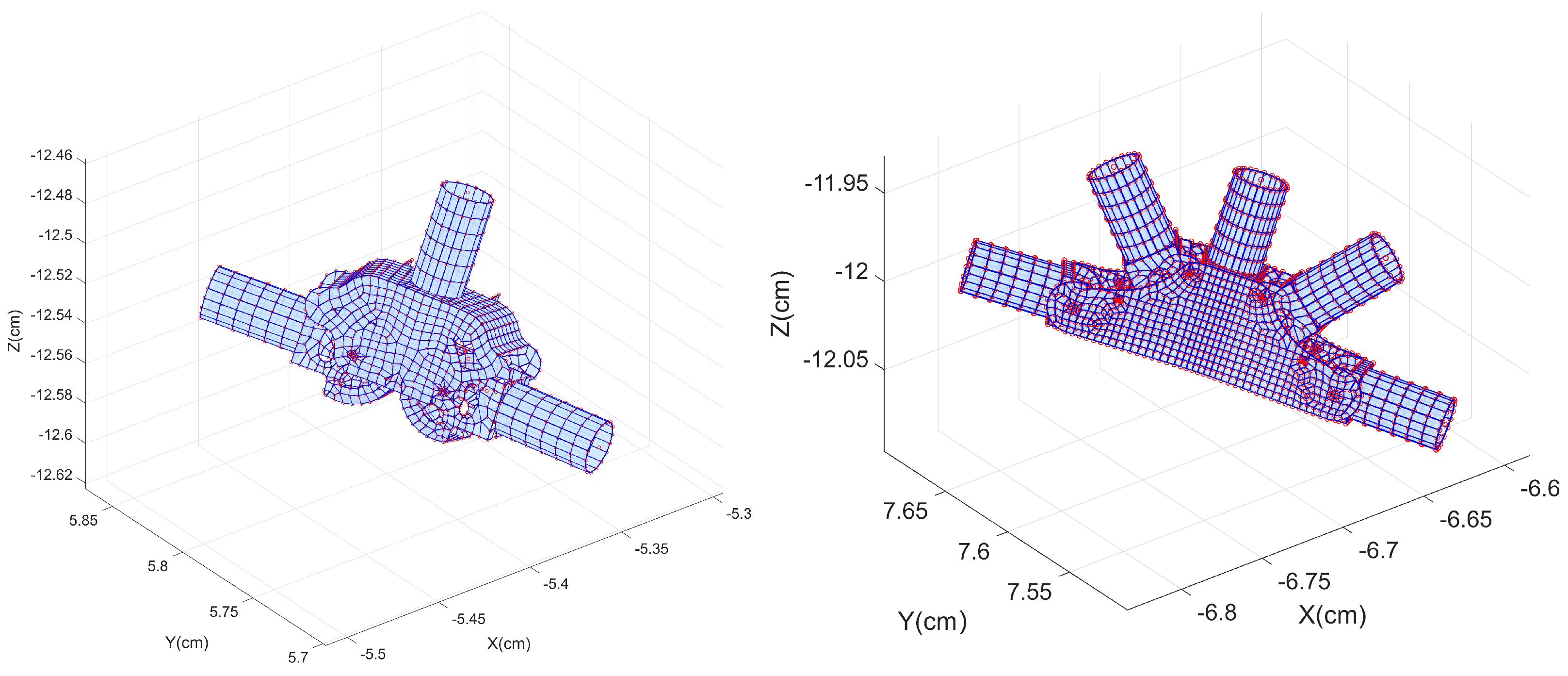
Figure 9 presents the refined finite element mesh of the deployment joint using the 3D thick cylindrical shell ANCF element defined in Section 2.1.1. Dynamic simulation under ideal conditions (no thermal load, no clearance) demonstrates that the displacement and velocity responses of the joint branches agree excellently with theoretical analytical solutions with a relative end-positioning error below 0.5%. This confirms the basic accuracy of the proposed ANCF framework for rigid–flexible coupling motion in deployable mechanisms and establishes a reliable benchmark for the subsequent validation of thermal and clearance nonlinearity effects.

4.1.2. Pure Thermal Effect Validation

This section verifies the accuracy of the proposed thermo-mechanical coupling module and temperature-dependent hinge kinematic model by quantifying the thermally induced rotational response of two typical deployment hinges (triangular and pentagonal) under extreme thermal loads. Simulation results are compared against thermal–structural coupling solutions from the commercial software ABAQUS 2025 to validate the prediction precision of temperature effects on hinge kinematic behavior.

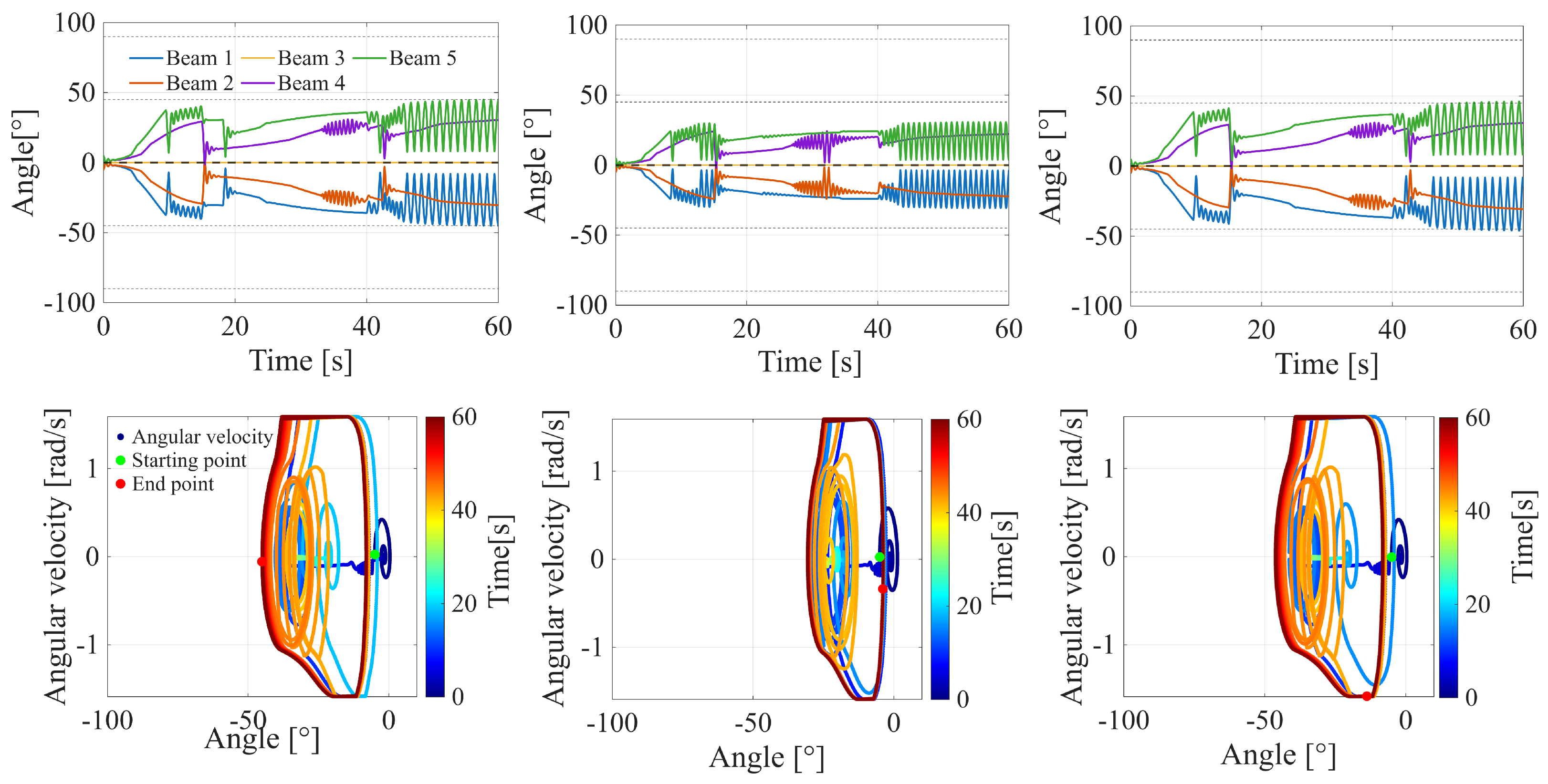
Figure 10 illustrates the dynamic response of the triangular deployment hinge under uniform temperature rises of $\Delta T=55 °\mathrm{C}$, $105 °\mathrm{C}$, and $155 °\mathrm{C}$ (left to right columns). Upper subplots show the 0–60 s rotational angle time histories for the five kinematic branches; response discrepancies arise from distinct constraint boundaries and thermal expansion degrees of freedom. As $\Delta T$ increases, the maximum rotational angle rises monotonically from 18.7° to 52.4°, which is accompanied by amplified vibration amplitude and accelerated fluctuation frequency—driven by the temperature-dependent reduction in Young’s modulus of 6061-T6 aluminum alloy, which weakens structural stiffness. The proposed model shows excellent agreement with ABAQUS simulations with a maximum relative error below 1.2% across all cases. Lower subplots depict phase trajectories (angular velocity vs. rotational angle) with the color bar indicating elapsed time (dark blue: 0 s; bright red: 60 s). Red and green markers denote initial and final states, respectively. With elevated temperature, the phase envelope expands significantly, and the peak angular velocity increases from $0.52\mathrm{rad}/\mathrm{s}$ ($\Delta T=55 °\mathrm{C}$) to $1.38\mathrm{rad}/\mathrm{s}$ ($\Delta T=155 °\mathrm{C}$). The increased number of trajectory loops confirms enhanced nonlinear dynamic response under higher thermal loads, while the smooth, closed trajectories verify the model’s stability and accuracy in capturing thermally induced behavior without spurious numerical oscillations.

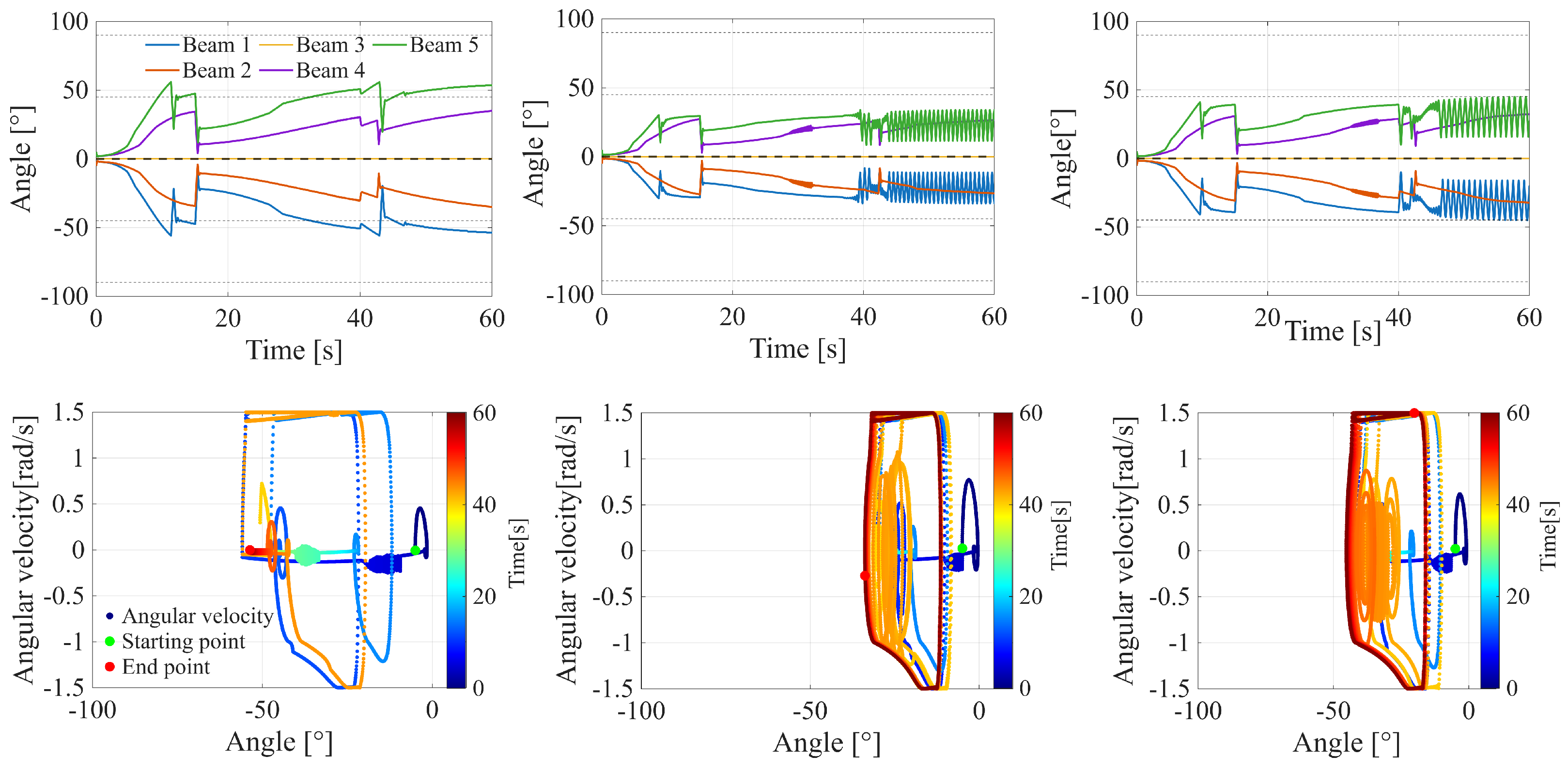
Figure 11 illustrates the dynamic response of the pentagonal deployment hinge under axial temperature gradients of 5 °C/mm, 10 °C/mm, and 15 °C/mm (left to right columns). Upper subplots show the 0–60 s rotational angle time-histories for the five kinematic branches; response discrepancies arise from non-uniform temperature distribution causing differential thermal expansion, uneven bending moments, and branch-specific constraint stiffness. As the gradient increases, the maximum angular difference between adjacent branches rises monotonically from 16.2° to 47.6°, accompanied by intensified high-frequency fluctuations—driven by amplified non-uniform thermal loads and temperature-dependent stiffness reduction. The proposed model agrees well with ABAQUS simulations with a maximum relative error below 3% across all cases. Lower subplots depict phase trajectories (angular velocity vs. rotational angle) with the color bar indicating elapsed time (dark blue: 0 s; bright red: 60 s). Red and green markers denote initial and final states, respectively. With steeper gradients, the phase envelope expands markedly, and peak angular velocity increases from $0.48\mathrm{rad}/\mathrm{s}$ (5 °C/mm) to $1.42\mathrm{rad}/\mathrm{s}$ (15 °C/mm). The increased loop count and distorted features confirm stronger nonlinear behavior under non-uniform thermal fields, while the smooth trajectory evolution verifies the model’s stability and accuracy.

4.1.3. Pure Clearance Effect Validation

The correctness of the nonlinear clearance hinge contact force model is verified through the classic slider–crank mechanism benchmark with a revolute joint clearance of 0.1 mm. The dynamic response of the mechanism is calculated using the proposed model, and the results are compared with the classic experimental data published by Flores et al. [6].

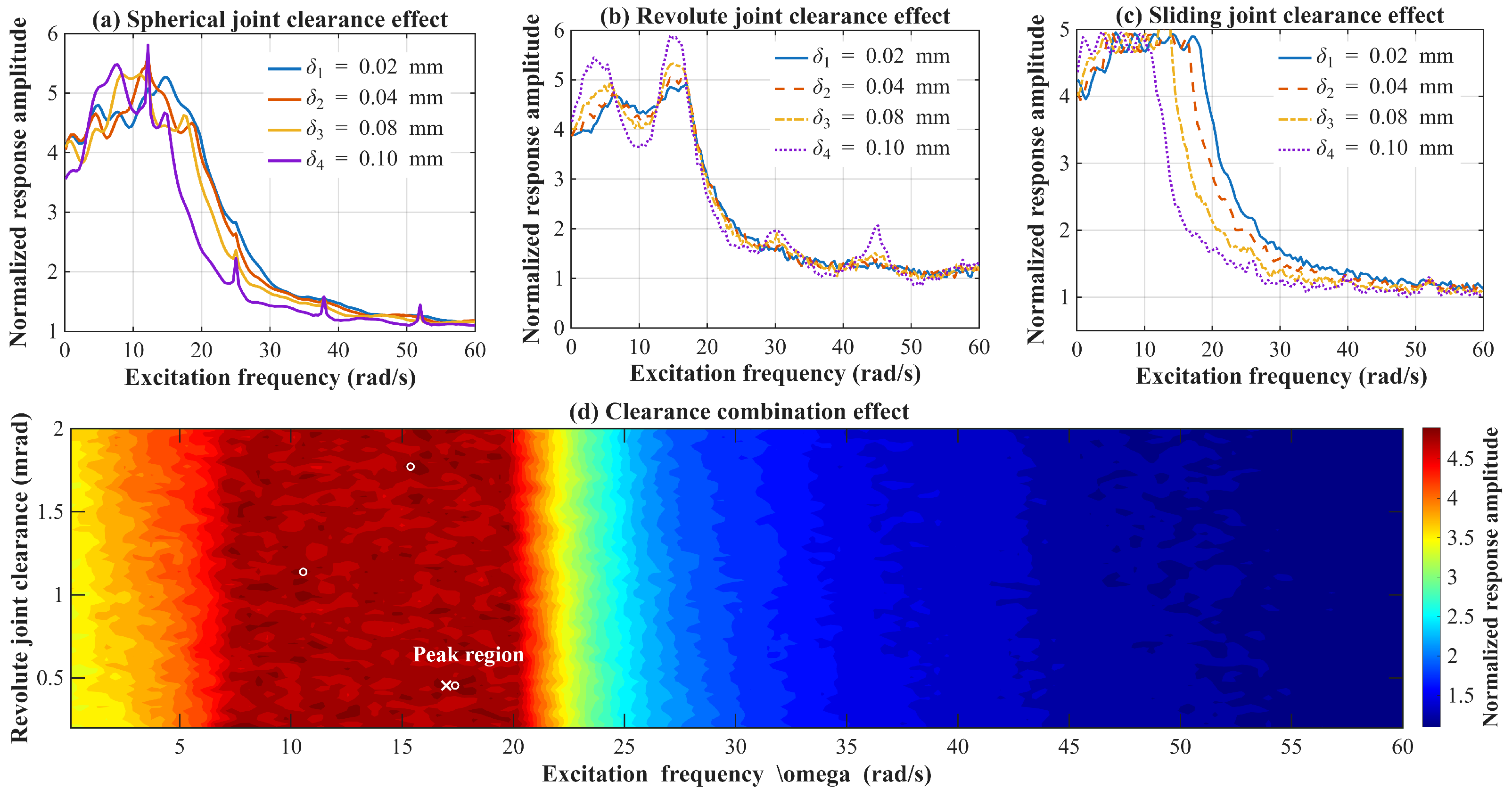
Figure 12 quantifies the influence of clearance joint type, size, and excitation frequency on dynamic response, comprising three single-clearance subplots (a–c, upper row) and one combined-effect contour plot (d, lower row). Subplots (a), (b), and (c) present normalized response amplitude versus excitation frequency (0–$60\mathrm{rad}/\mathrm{s}$) for spherical, revolute, and translational joints, respectively, under four radial clearance sizes: ${\delta }_1=0.02\mathrm{mm}$ (blue solid), ${\delta }_2=0.04\mathrm{mm}$ (orange dashed), ${\delta }_3=0.08\mathrm{mm}$ (yellow dash-dot), and ${\delta }_4=0.10\mathrm{mm}$ (purple dotted). For all joint types, the peak normalized amplitude increases monotonically with clearance size while the resonance peak shifts toward lower frequencies. As clearance increases from $0.02$ to $0.10\mathrm{mm}$, the peak amplitude rises from $5.1$ to $5.8$ (spherical), $4.8$ to $5.4$ (revolute), and $4.9$ to $5.1$ (sliding). All curves exhibit a dominant resonance near $10\mathrm{rad}/\mathrm{s}$ followed by gradual decay. The predicted contact forces and vibration frequencies agree well with experimental data from Flores et al. [6] with a maximum relative error below $4\%$. Subplot (d) shows the combined effect of revolute joint clearance ($0.2$–$2.0\mathrm{mrad}$) and excitation frequency (0–$60\mathrm{rad}/\mathrm{s}$) on normalized response amplitude (color bar: $1.0$–$4.5$). The peak response region (5–$20\mathrm{rad}/\mathrm{s}$, $0.2$–$1.8\mathrm{mrad}$) confirms that clearance–resonance coupling significantly amplifies system dynamics. This validation demonstrates that the proposed clearance contact model accurately captures nonlinear contact–impact behavior across different clearance joint types in deployable mechanisms.

4.1.4. Full Model Validation

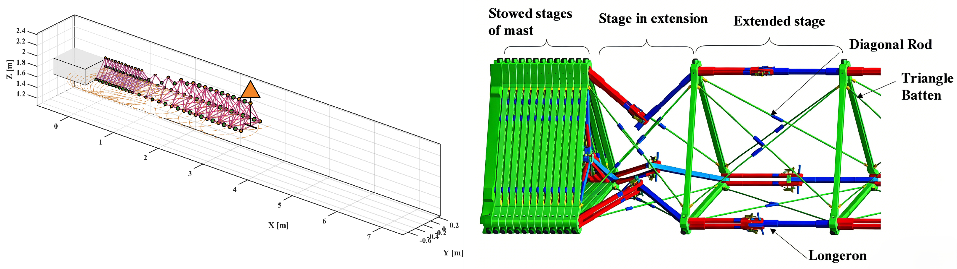
Given the prohibitive cost and logistical constraints of full-scale on-orbit validation for the pre-research annular truss antenna, validation relies on the benchmark deployable mast of Shimizu et al. [41], which provides systematic thermal radiation tests and repeatable stick–slip response data. The proposed unified thermo-tribological stick–slip model is benchmarked against ABAQUS simulations (user-defined temperature-dependent and classical Coulomb friction models) and published experimental results to confirm its fidelity in capturing thermally excited nonlinear dynamics.

Figure 13 shows a full model validation. The left panel shows a three-dimensional finite element model of the ASTRO-H imitating deployable mast, where the orange marker indicates the end displacement measurement point that matches the benchmark sensor layout. The right panel displays a structural schematic adapted from Shimizu et al. [41], illustrating the deployment stages and core components of the experimental prototype. Validation uses the reference condition: 0–600 s radiation heating (from 20 °C to 70 °C), 600–1200 s natural cooling, and 0.5 mm pin–longeron joint clearance. The proposed unified thermo-tribological stick–slip model (with sticking time-dependent static friction and temperature-dependent friction coefficient) is solved via HHT-$\alpha$ ($\alpha =-0.1$) and compared against ABAQUS VFRIC simulations and experimental data; key indices are listed in

Table 6. Full model validation and error comparison: (A) Experimental Data; (B) Proposed Unified Thermo-Tribological Model; (C) ABAQUS User-Defined Temperature-Dependent Friction Model; (D) ABAQUS Native Classic Coulomb Model.

Index	A	B	Error A vs. B	C	Error A vs. C	D	Error A vs. D
Maximum Y-direction End Displacement/mm	1.212	1.214	0.16%	1.268	4.62%	1.387	14.44%
Peak Y-direction Acceleration/mm · s−2	14.71	14.96	1.70%	15.52	5.51%	34.75	136.23%
Occurrence Timeof Peak Acceleration/s	460	454	1.30%	437	5.00%	569	23.70%
Peak Contact Pressure at Sliding Joint/MPa	0.872	0.883	1.26%	0.915	4.93%	1.068	22.48%

.

The unified model modifies the reference rising static friction formulation with temperature-dependent correction:

$${\mu }_s(\tau ,T)={\mu }_{s\infty }\left(T\right)-\left({\mu }_{s\infty }\left(T\right)-{\mu }_k\left(T\right)\right)exp\left(-\gamma {\tau }^m\right)$$

$${\mu }_{s\infty }\left(T\right)={\mu }_{s\infty ,0}\left[1+{\alpha }_T\left(T-T_0\right)\right],{\mu }_k\left(T\right)={\mu }_{k,0}\left[1+{\beta }_T\left(T-T_0\right)\right]$$

where ${\mu }_{s\infty ,0}=0.0859$ and ${\mu }_{k,0}=0.0623$ are the reference friction coefficients at room temperature $T_0=20 °\mathrm{C}$ identified by the friction experiment in the reference document, ${\alpha }_T$ and ${\beta }_T$ are the temperature influence coefficients of static and kinetic friction coefficients obtained by temperature-dependent friction calibration, and $\gamma =0.570$, $m=0.629$ are the sticking time-dependent parameters fully consistent with the reference document.

Validation results demonstrate that the proposed unified thermo-tribological coupling model—which fully incorporates sticking time-dependent friction evolution and temperature-dependent friction coefficient correction—achieves <2% error relative to experimental data across all core dynamic indices, enabling a high-fidelity reproduction of thermally induced stick–slip phenomena. The ABAQUS user-defined temperature-dependent friction model reduces errors from 14–$136\%$ to <6% compared with the classical Coulomb model, confirming that temperature-dependent friction characteristics effectively mitigate simulation errors. Nevertheless, the proposed model retains a distinct accuracy advantage by further accounting for time-varying static friction evolution during sticking, underscoring its superiority for nonlinear thermally induced stick–slip dynamics in flexible deployable space structures with clearance joints and providing a high-precision tool for disturbance suppression design.

4.2. Dynamic Response Analysis of Three Deployment Configurations

Based on the validated model, the dynamic response of the antenna under three typical deployment configurations—a secondary arm extending from the interior of the main boom, secondary arm deployment, and reflector deployment—is calculated and analyzed in detail with the reference parameters listed in Table 4.

4.2.1. Configuration 1: Secondary Arm Extending from the Interior of the Main Boom

Configuration 1 models the 720 s constant-speed (0.1 m/s) translation of a 63.5 m secondary arm from a 65.5 m main boom. The system is subjected to a transient thermal load (−100 °C to 50 °C at 15 °C/s, mimicking Earth-shadow entry/exit) and incorporates a 0.1 mm translational joint clearance. Temperature-dependent material properties and clearance-induced contact nonlinearity jointly govern translation stability and potential thermally induced vibration. Validation focuses on the consistency of simulated displacement and velocity with theoretical predictions under thermo-tribological coupling effects.

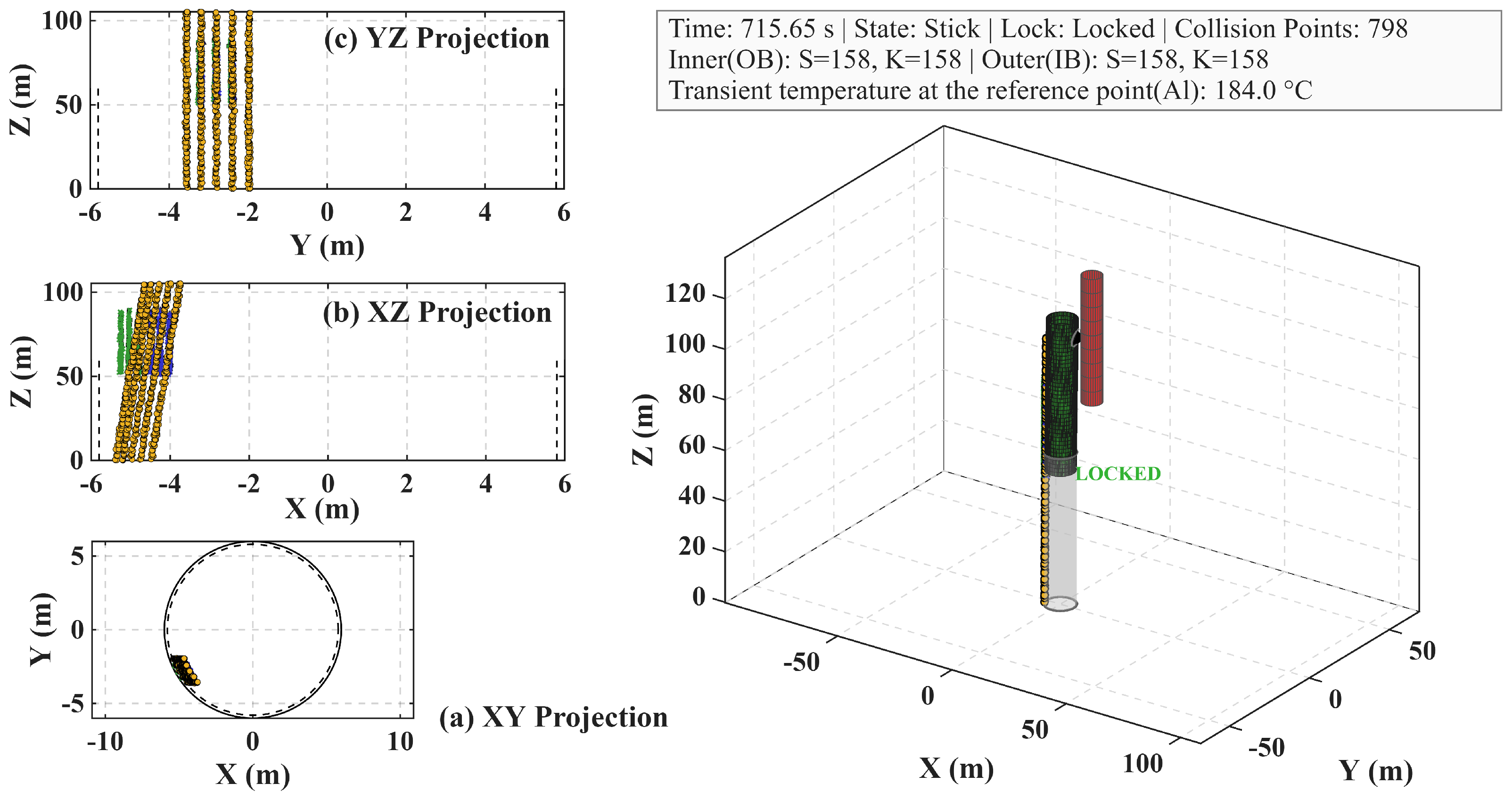
Figure 14 illustrates the deployment state at $t=715.65\mathrm{s}$ (near the stroke end of $720\mathrm{s}$). The right panel presents a three-dimensional view of the fully extended secondary arm (red) and the main boom (black-green), where the system is in the “LOCKED” state at 184.0 °C with 798 collision points and consistent OB/IB element counts $S=158$, $K=158$. The left panel shows three orthogonal projections: (a) XY, (b) XZ, and (c) YZ, where orange dots denote contact collision points, and green and blue lines represent the profiles of the secondary arm and main boom, respectively. The lateral offset remains within $\pm 0.5\mathrm{m}$, and the axial stroke reaches $63.5\mathrm{m}$ with a positioning error below $0.2\%$, confirming the accuracy of the proposed model.

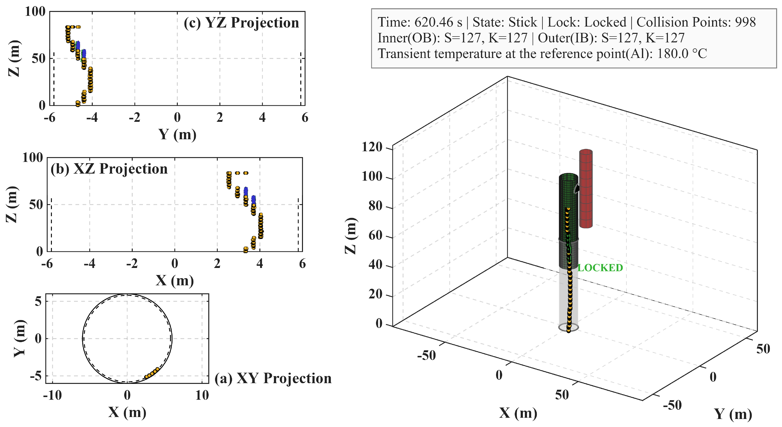
Figure 15 shows the system state at the intermediate deployment stage $t=620.46\mathrm{s}$. The right panel presents a three-dimensional view of the partially extended main boom (black-green) and secondary arm (red), where the joint is in the stick phase at 180.0 °C with 998 collision points and consistent OB/IB element counts $S=127$, $K=127$. The left panel provides three orthogonal projections (XY, XZ, YZ), where orange dots indicate a non-uniform contact distribution caused by thermal deformation and clearance misalignment. The lateral offset reaches $\pm 1.2\mathrm{m}$, and the axial stroke is $54.2\mathrm{m}$. The elevated contact count relative to the final stage reflects intensified intermediate contact–impact behavior.

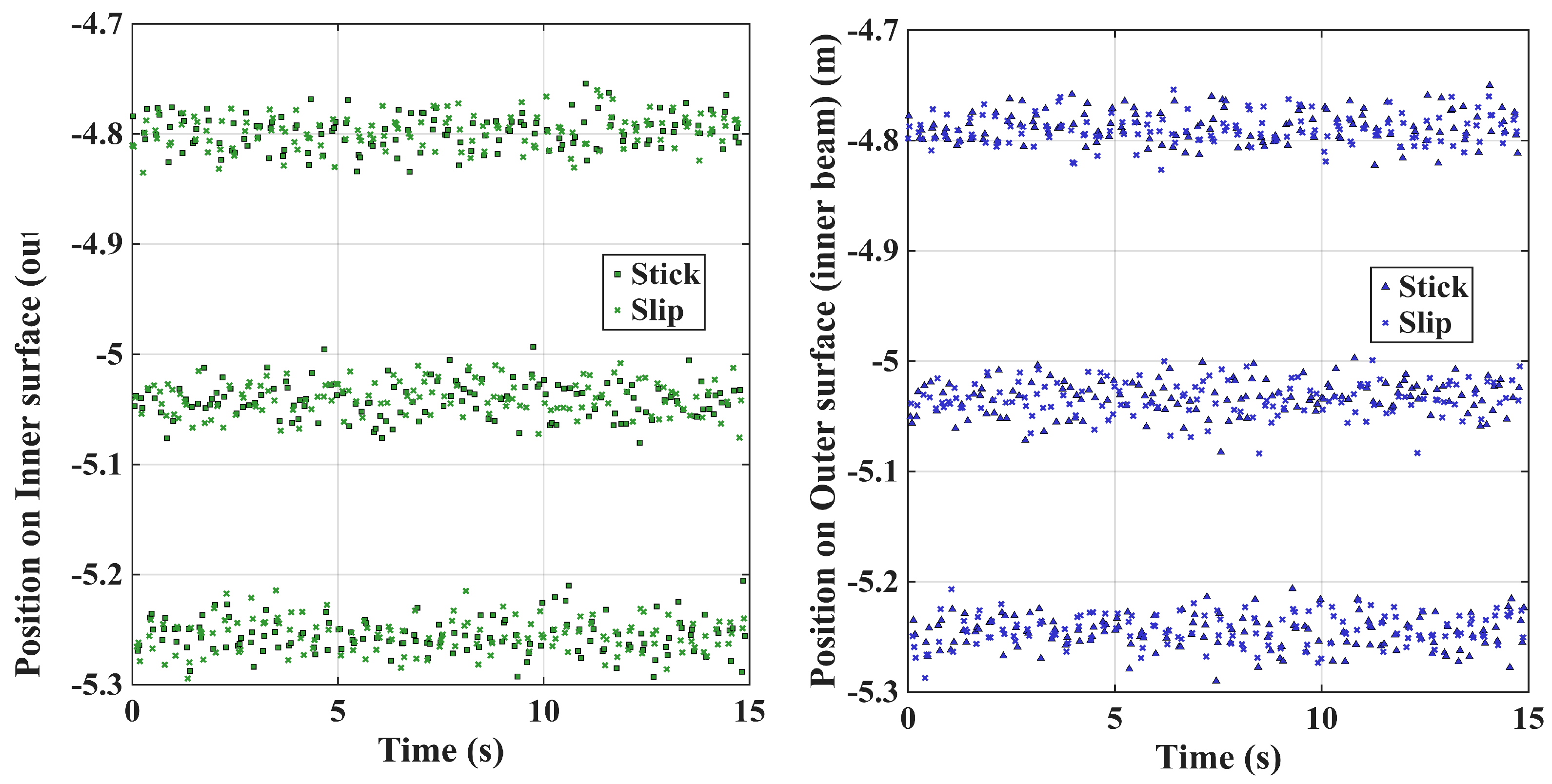
Figure 16 illustrates the contact state distribution during the initial deployment phase from 0 to $15\mathrm{s}$. The left subfigure corresponds to the outer surface of the inner beam, where green squares denote stick and green crosses denote slip; contact occurs at positions $-4.8$, $-5.0$, and $-5.2$ to $-5.3\mathrm{m}$ with slip accounting for approximately $45\%$ of the contact area. The right subfigure shows the inner surface of the outer beam, where blue triangles indicate stick and blue crosses indicate slip; slip is concentrated at $-4.8$ and $-5.0\mathrm{m}$, accounting for about 28% of the contact area. The asymmetric stick–slip behavior arises from thermal expansion gradients and clearance misalignment. The continuous coexistence of stick and slip confirms strong thermo-tribological coupling, where thermal deformation drives slip even under nominally locked conditions.

4.2.2. Configuration 2: Secondary Arm Deployment

Configuration 2 models the 567 s constant-speed ($0.05\mathrm{rad}/\mathrm{s}$) rotation of the 63.5 m secondary arm following full extension. The system is subjected to a 50 °C/m temperature gradient (root-to-tip thermal differential) and incorporates a $0.05\mathrm{mm}$ rotation joint clearance. Dynamic analysis focuses on temperature-gradient effects on stiffness and the thermal bending moment, clearance-induced contact nonlinearity, angular velocity stability, and thermally induced stick–slip behavior at the joint—the latter directly affecting rotational positioning accuracy.

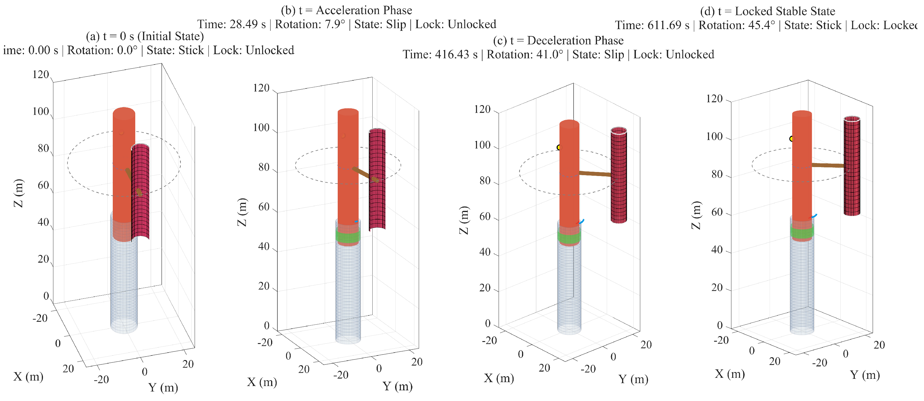
Figure 17 illustrates the four key stages of the secondary arm’s rotational deployment around the main boom from the initial to the fully locked state. (a) In the initial state ($t=0\mathrm{s}$), the secondary arm (red cylinder) is stowed with 0° rotation, the joint is in the stick state, and the lock mechanism is unlocked. (b) In the acceleration phase ($t=28.49\mathrm{s}$), the arm rotates to 7.9°, enters the slip state, and accelerates outward. (c) In the deceleration phase ($t=416.43\mathrm{s}$), rotation reaches 41.0°, and the arm decelerates while remaining in the slip state. (d) In the locked stable state ($t=611.69\mathrm{s}$), the arm completes deployment at 45.4°, locks in the stick state, and reaches its final position.

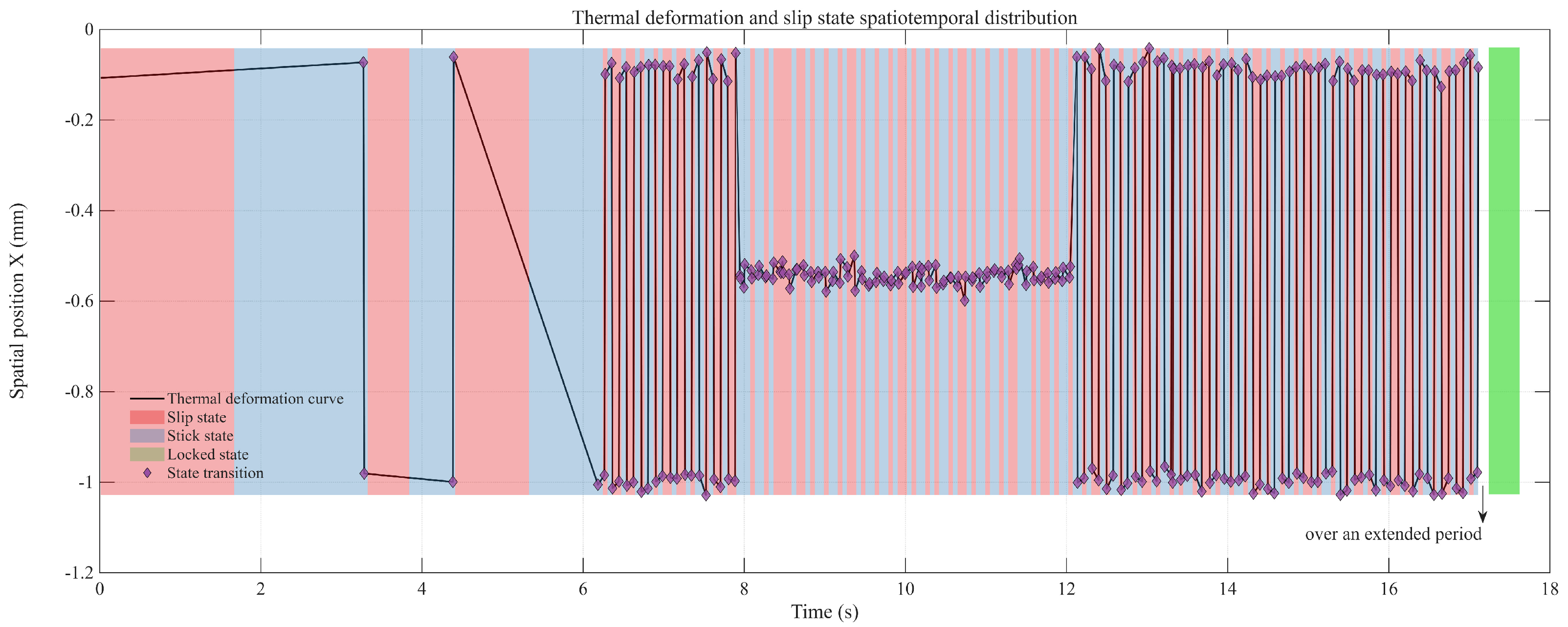
Figure 18 illustrates the spatiotemporal distribution of thermal deformation and stick–slip states of the clearance joint (Configuration 2). The black line shows the thermal deformation curve of the contact surface with the vertical axis representing the spatial position X (mm). Red and light blue shaded regions denote slip and stick states, respectively, and purple diamonds mark stick–slip transitions. Before $t=6\mathrm{s}$, the joint alternates between stick and slip with a slow change in thermal deformation. After $t=6\mathrm{s}$, frequent stick–slip oscillations occur due to coupled thermal deformation and contact friction. The deformation amplitude stabilizes around $0.95\mathrm{mm}$, and transitions concentrate at the upper and lower deformation limits, reflecting the self-locking and unlocking behavior of the clearance joint under thermal loads.

4.2.3. Configuration 3: Reflector Deployment

Configuration 3 models the 6000 s combined rotation–translation deployment of the 100 m diameter ring truss reflector under constant angular acceleration ($0.01\mathrm{rad}/{\mathrm{s}}^2$). The system experiences extreme thermal shock (200 °C to −50 °C at 25 °C/s, simulating shadow entry) and incorporates uniform 0.03 mm joint clearances across multiple revolute and translational joints. Dynamic analysis addresses thermo-mechanical coupling under combined motion, including extreme-temperature-induced nonlinear behavior, cumulative multi-joint clearance effects, and thermal stress/contact force distributions. This configuration exhibits the highest sensitivity to thermal and clearance effects among the three stages, providing essential theoretical support for surface accuracy control and disturbance suppression.

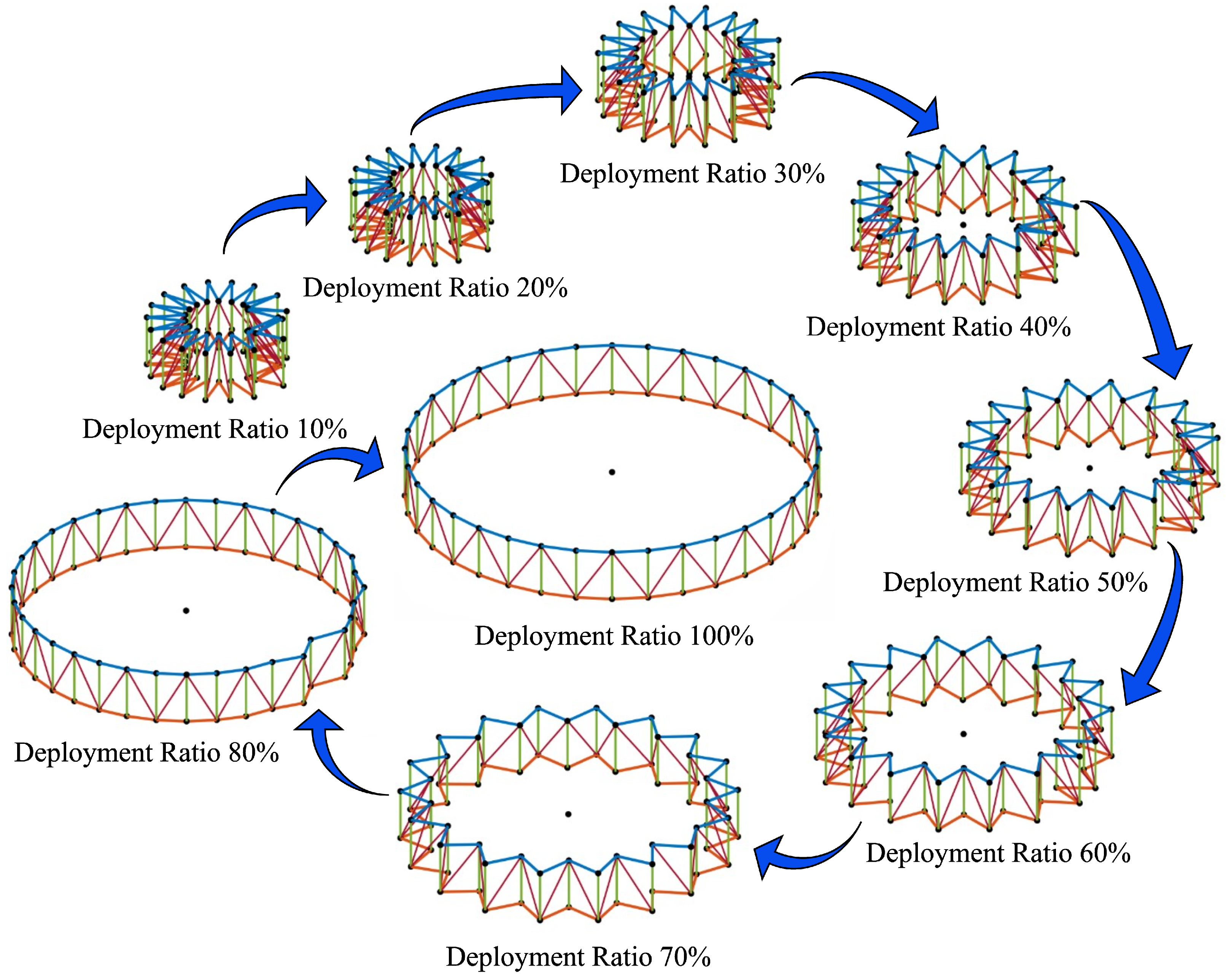
Figure 19 shows the deployment sequence of the ring truss antenna with expansion ratios ranging from $10\%$ to $100\%$. Circumferential battens, radial struts, and diagonal ties are depicted in blue, red, and green, respectively. The truss expands from a folded star-like profile (10–$40\%$) through a polygonal intermediate stage (50–$80\%$) to a fully circular rigidized configuration ($100\%$). The uniform symmetric expansion, marked by blue arrows, confirms the geometric validity of the deployment mechanism.

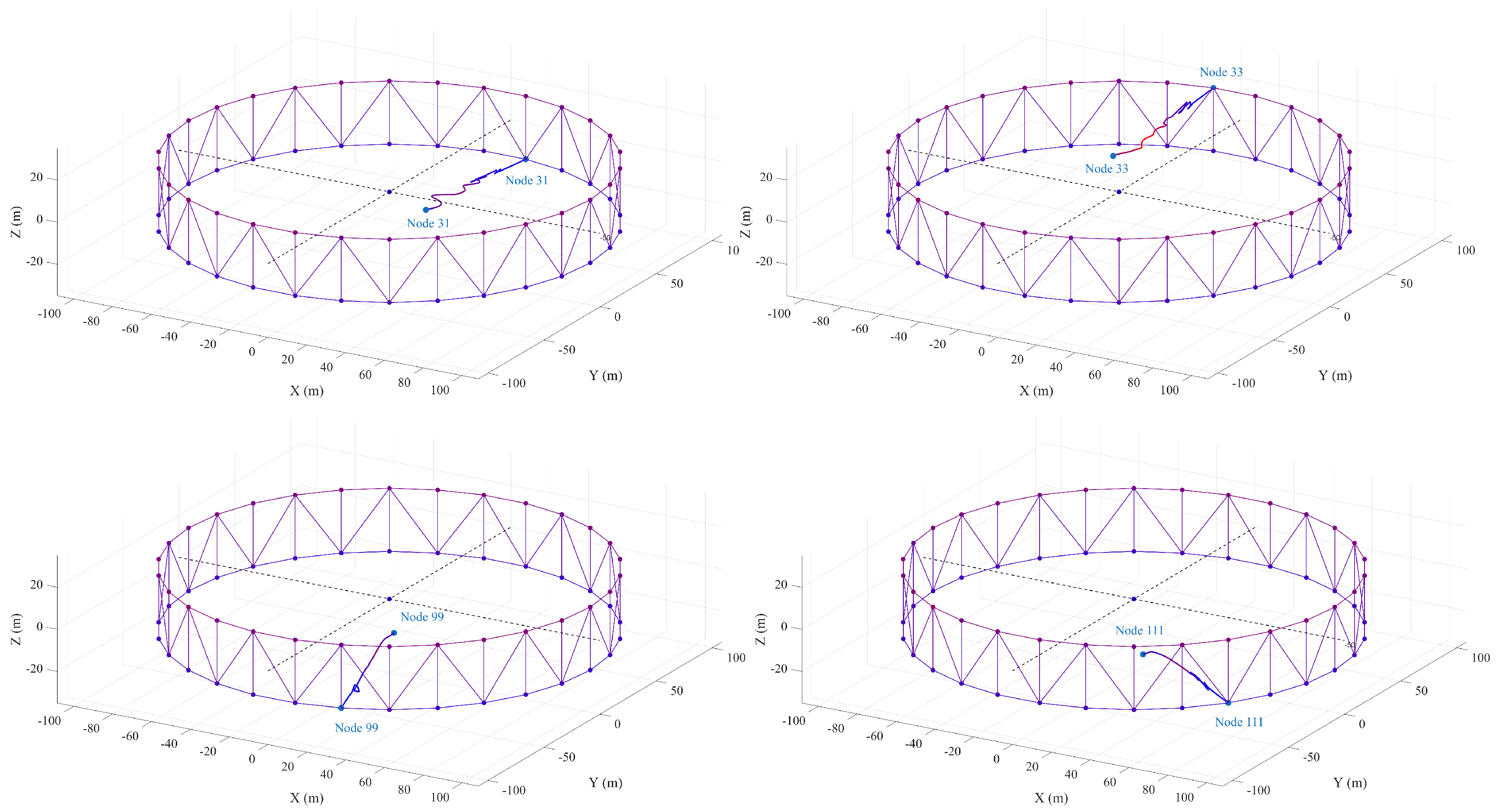
Figure 20 illustrates the node trajectories and thermal deformation of the ring truss antenna at key nodes under orbital thermal loads (Configuration 3). In the fully deployed ring truss model, purple lines represent truss members, and purple/blue dots represent structural nodes. Blue and red trajectories, respectively, show the displacements of key nodes (31, 33, 99, 111) under low and high temperatures with red indicating enhanced thermal drift. Radial nodes 31 and 33 undergo larger in-plane drift, whereas chord nodes 99 and 111 exhibit significant out-of-plane deformation. The maximum thermal displacement reaches $2.1\mathrm{m}$ under high temperature, reflecting asymmetric thermal deformation that compromises shape accuracy.

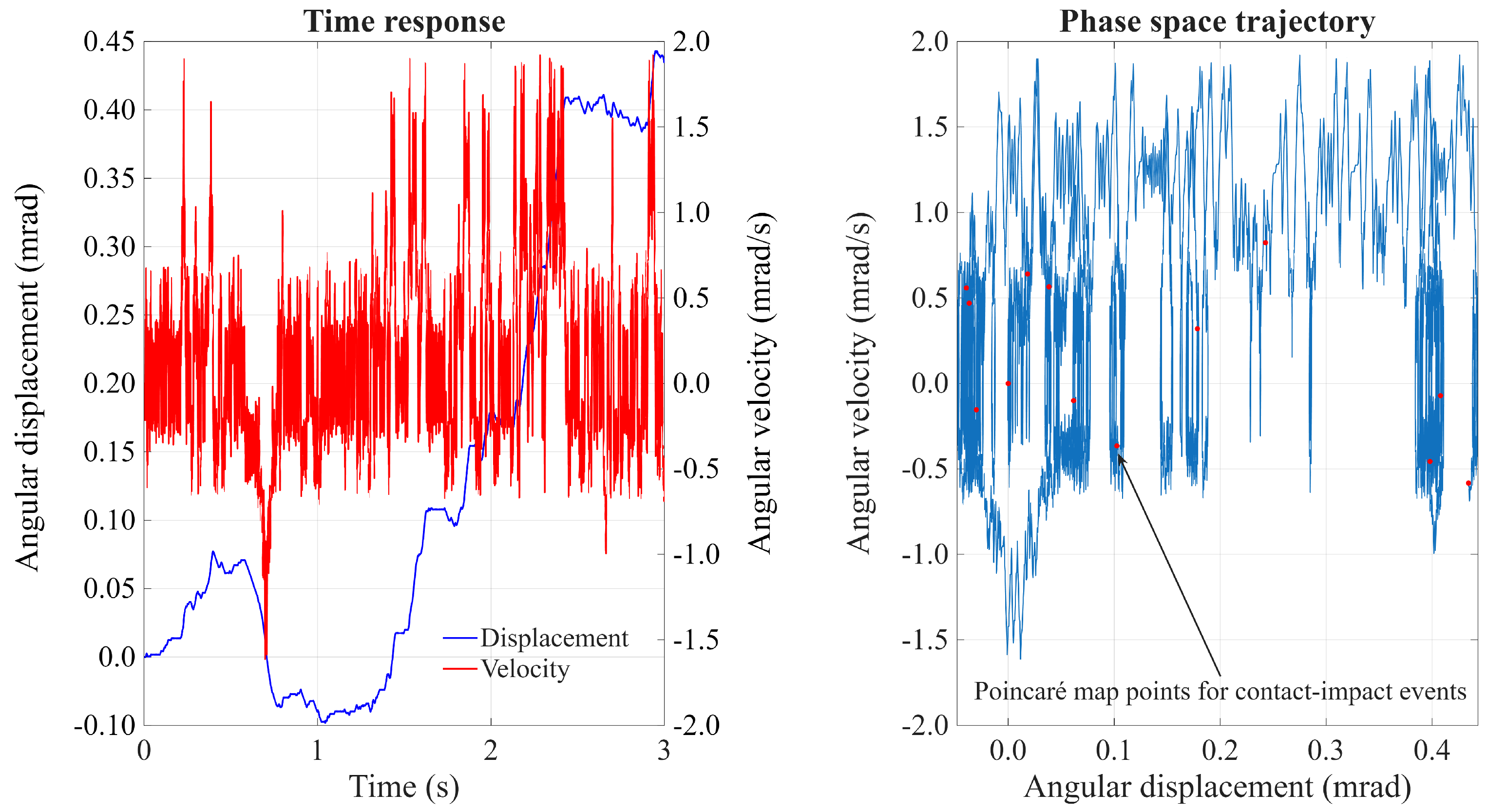
Figure 21 illustrates the time response and phase space trajectory of the ring truss antenna joint under thermo-clearance coupling excitation. In the left subplot, the blue and red lines, respectively, denote the angular displacement ($\mathrm{mrad}$) and angular velocity ($\mathrm{mrad}/\mathrm{s}$). The right subplot shows the corresponding phase space trajectory (angular velocity versus angular displacement). The time response exhibits a baseline drift from $-0.1$ to $0.5\mathrm{mrad}$ in displacement along with high-frequency velocity fluctuations caused by clearance-induced impacts. The phase trajectory forms scattered, non-periodic loops, confirming strong nonlinear stick–slip behavior under thermally amplified clearance effects. The red markers indicate the key transition points between stick and slip states.

4.3. Parametric Sensitivity Analysis

To quantitatively analyze the influence of temperature and clearance parameters on the deployment dynamic characteristics of the antenna, a single-factor parametric sensitivity analysis is carried out with the secondary arm extending from the interior of the main boom configuration as the research object, and the influence law of temperature range, clearance size, and friction coefficient on the system dynamic response is revealed.

4.3.1. Influence of Temperature Range

The ambient temperature range is set from −200 °C to 200 °C, covering the extreme cyclic temperature fluctuation of the GEO space environment. The variation of the main boom end displacement, first-order natural frequency, and thermal-induced vibration amplitude with temperature is listed in

Table 7. Influence of temperature on the dynamic characteristics of the main boom.

Temperature °C	End Displacement m	First-Order Natural Frequency Hz	Vibration Mplitude mm
−200	2.5000	18.5	2.5
−100	2.5075	17.9	3.1
25	2.5200	16.8	4.2
100	2.5300	16.2	5.0
200	2.5350	16.5	5.5

.

The results in Table 7 demonstrate the influence of temperature on the main boom’s static and dynamic responses. As the temperature increases from −200 °C to 200 °C, the end displacement rises moderately by $1.4\%$ (from $2.5000\mathrm{m}$ to $2.5350\mathrm{m}$). This increase is primarily caused by axial thermal expansion with a smaller contribution from thermally induced bending due to non-uniform temperature distribution. The first-order natural frequency decreases by $10.8\%$ (from $18.50\mathrm{Hz}$ to $16.50\mathrm{Hz}$), which correlates well with the temperature-dependent reduction in Young’s modulus of the aluminum alloy 6061-T6 (approximately 9–$12\%$ over the same temperature range). The thermally induced vibration amplitude increases by $120\%$ (from $2.5\mathrm{mm}$ to $5.5\mathrm{mm}$), indicating that higher temperatures not only soften the structure but also intensify the thermal excitation, leading to a significantly amplified dynamic response.

These trends are physically consistent with the material’s thermomechanical behaviour and provide a reliable basis for engineering design under extreme thermal environments.

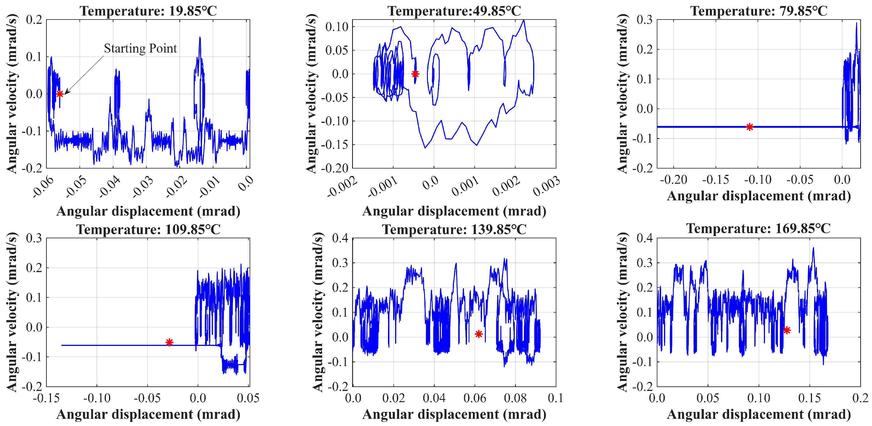
Figure 22 consists of six subplots corresponding to temperatures of (a) 19.85 °C, (b) 49.85 °C, (c) 79.85 °C, (d) 109.85 °C, (e) 139.85 °C, and (f) 169.85 °C. Blue curves depict angular velocity versus angular displacement phase trajectories with red stars marking the initial state. At 19.85 °C (a), the trajectory exhibits a compact, weakly nonlinear loop, reflecting high material stiffness and minimal thermal-expansion-induced clearance with motion dominated by low-amplitude stick–slip. As temperature increases to 49.85 °C (b) and 79.85 °C (c), the trajectory expands and becomes increasingly irregular due to progressive thermal softening and clearance enlargement, leading to more frequent slip events and impact-induced velocity spikes. At 109.85 °C (d), the envelope expands markedly with sharp velocity spikes, signaling a transition from stable stick–slip to impact-dominated motion as thermally induced clearance reaches a critical threshold. At 139.85 °C (e) and 169.85 °C (f), the trajectories exhibit severe chaotic behavior with expanded loops and extreme velocity fluctuations; drastically reduced stiffness and maximized clearance cause the joint to operate in a fully nonlinear regime dominated by continuous impacts and tangential slip.

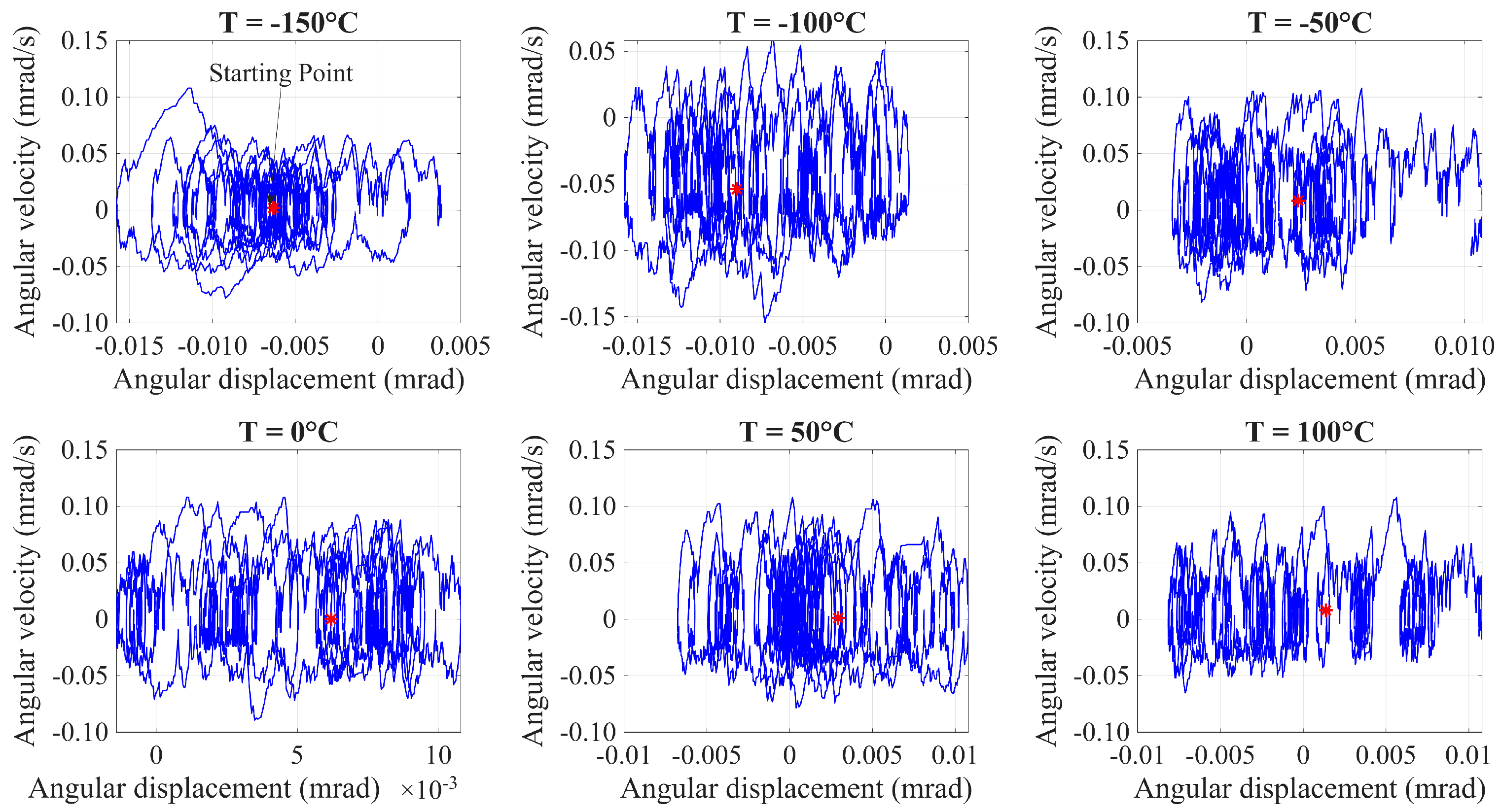
Figure 23 consists of six subplots corresponding to temperatures of (a) −150 °C, (b) −100 °C, (c) −50 °C, (d) 0 °C, (e) 50 °C, and (f) 100 °C. Blue curves depict angular velocity versus angular displacement phase trajectories with red stars marking the initial state. At cryogenic temperatures (−150 °C), the trajectory exhibits a compact, weakly nonlinear loop, reflecting high stiffness and thermal contraction that suppresses impacts and limits slip motion. As temperature increases to −100 °C and −50 °C, the envelope progressively expands with increased irregularity due to reduced stiffness and diminished thermal contraction, allowing more frequent slip events and impact-induced velocity spikes. At 0 °C, a complex multi-looped structure emerges with moderate nonlinearity driven by nominal clearance and balanced stiffness. At elevated temperatures (50 °C and 100 °C), the trajectories become highly expanded and chaotic with large velocity fluctuations; significant thermal expansion maximizes effective clearance while drastically reduced stiffness permits unconstrained motion, resulting in a fully nonlinear regime dominated by continuous high-energy impacts and slip.

Temperature thus exerts two competing effects: (1) thermal expansion/contraction modifies effective clearance, and (2) temperature-dependent material properties alter structural stiffness. These synergistic effects govern the transition from compact, periodic trajectories at low temperatures to expanded, chaotic phase portraits at high temperatures.

4.3.2. Influence of Clearance Size

The radial clearance of the main boom revolute joint is set from 0.01 mm to 0.1 mm, covering the common clearance range of aerospace deployment hinges. The variation of the peak impact force at the clearance hinge and the angular velocity fluctuation amplitude with clearance size is listed in

Table 8. Influence of clearance size on the dynamic characteristics of the main boom.

Clearance Size mm	Peak Impact Force N	Angular Velocity Fluctuation rad/s
0.01	27.3	0.0042
0.02	38.6	0.0058
0.05	61.2	0.0087
0.08	76.5	0.0105
0.1	85.0	0.0120

, and the corresponding influence curves are shown in Figure 24.

Table 8 quantifies the effect of radial clearance size on the dynamic behavior of the main boom revolute joint. As the clearance increases from 0.01 mm to 0.10 mm, the peak impact force at the hinge rises by approximately $211\%$ (from $27.3\mathrm{N}$ to $85.0\mathrm{N}$), and the amplitude of angular velocity fluctuation increases by about $186\%$ (from $0.0042\mathrm{rad}/\mathrm{s}$ to $0.0120\mathrm{rad}/\mathrm{s}$). This trend is physically consistent: a larger clearance allows the journal to travel a longer free-flight distance within the bearing before contact, leading to a higher relative impact velocity and consequently more severe contact collisions. The intensified impacts excite stronger nonlinear dynamic responses, including larger fluctuations in angular velocity. These results highlight the importance of minimizing clearance size in deployable space mechanisms to reduce impact forces and improve deployment stability.

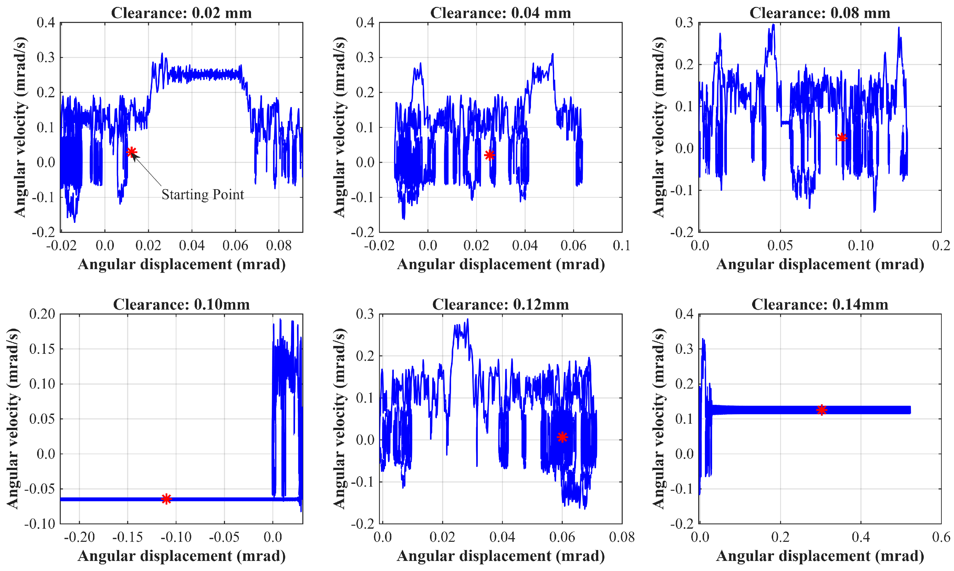
Figure 24 consists of six subplots corresponding to radial clearance sizes of (a) $0.02\mathrm{mm}$, (b) $0.04\mathrm{mm}$, (c) $0.08\mathrm{mm}$, (d) $0.10\mathrm{mm}$, (e) $0.12\mathrm{mm}$, and (f) $0.14\mathrm{mm}$. Blue curves depict angular velocity versus angular displacement phase trajectories with red stars marking the initial state. At minimum clearance ($0.02\mathrm{mm}$), the trajectory is compact and weakly nonlinear with motion dominated by continuous contact friction and weak stick–slip. As clearance increases to $0.04$–$0.08\mathrm{mm}$, the envelope expands with increased velocity spikes and irregular loops, reflecting intermittent separation and more frequent impact events. At $0.10\mathrm{mm}$, a distinct “flat-line” segment emerges, indicating a clear three-phase motion (contact, free flight, and impact) with a pronounced velocity jump upon impact. At $0.12\mathrm{mm}$, prolonged free flight leads to high-energy impacts and a highly chaotic, multi-looped response. At maximum clearance ($0.14\mathrm{mm}$), the trajectory is dominated by extended free-flight phases at near-constant velocity with only initial and terminal impact spikes, resulting in a simplified two-stage (impact–free flight–impact) response. Clearance size thus governs the transition from contact-dominated near-periodic motion at small clearances to impact- and free-flight-dominated dynamics at larger clearances.

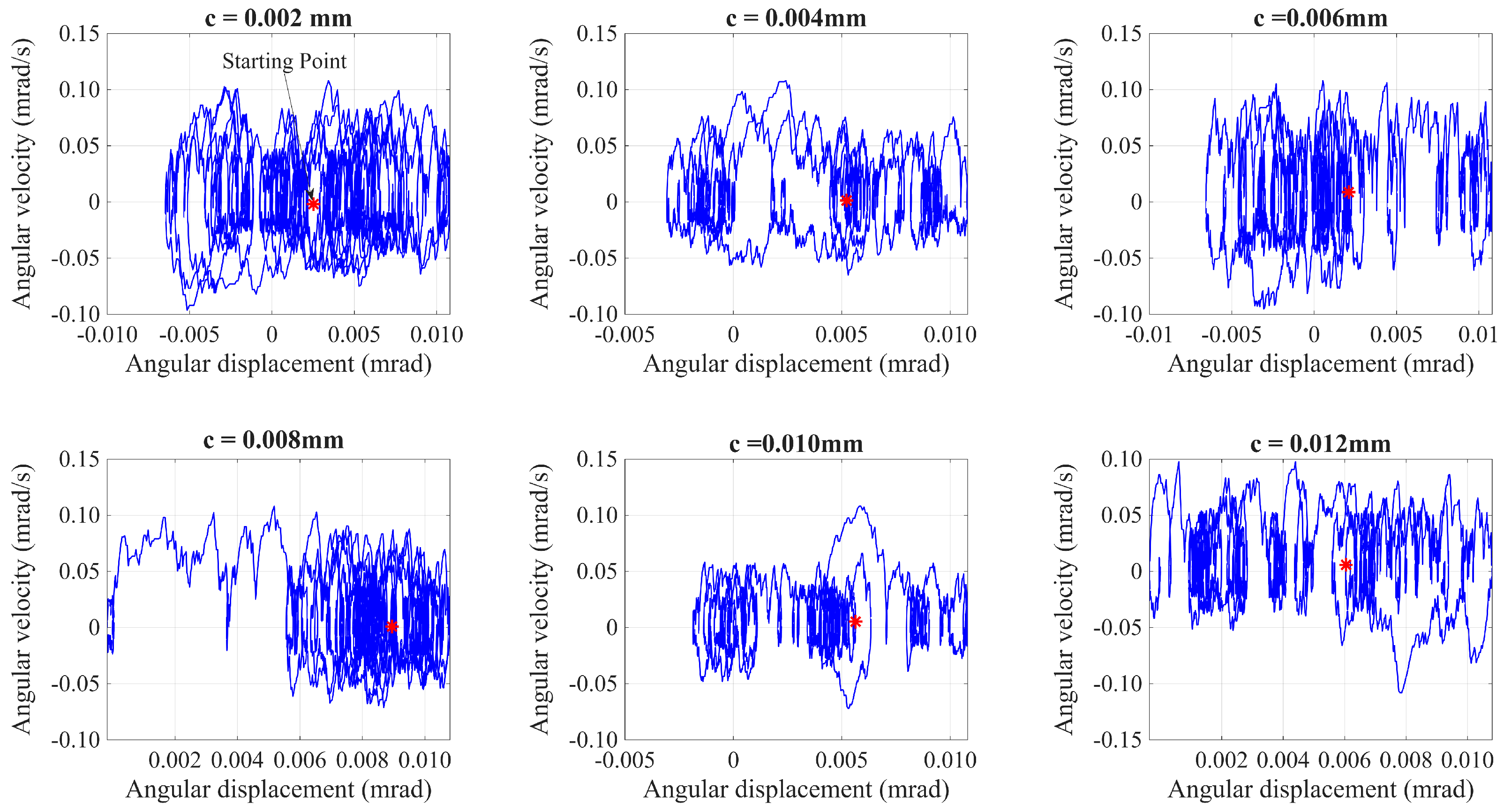
Figure 25 consists of six subplots corresponding to radial clearance sizes of (a) $c=0.002\mathrm{mm}$, (b) $0.004\mathrm{mm}$, (c) $0.006\mathrm{mm}$, (d) $0.008\mathrm{mm}$, (e) $0.010\mathrm{mm}$, and (f) $0.012\mathrm{mm}$. Blue curves depict angular velocity versus angular displacement phase trajectories with red stars marking the initial state. At minimum clearance ($0.002\mathrm{mm}$), the trajectory forms a compact, symmetric cloud, reflecting continuous contact and weak periodic stick–slip. As clearance increases to $0.004$–$0.006\mathrm{mm}$, the envelope expands with increased irregularity and velocity fluctuations, indicating intermittent separation and amplified impact intensity. At $0.008\mathrm{mm}$, a distinct three-phase behavior (contact, free flight, impact) emerges with elongated loops and sharp impact-induced velocity spikes. At $0.010$–$0.012\mathrm{mm}$, the trajectories become highly chaotic and expanded with large velocity swings and no clear periodicity; prolonged free flight and violent impacts drive a fully nonlinear, impact-dominated response. Clearance size thus governs the transition from contact-dominated near-periodic motion at small clearances to chaotic, impact- and inertia-driven dynamics at larger clearances.

4.3.3. Influence of Contact and Friction Coefficient

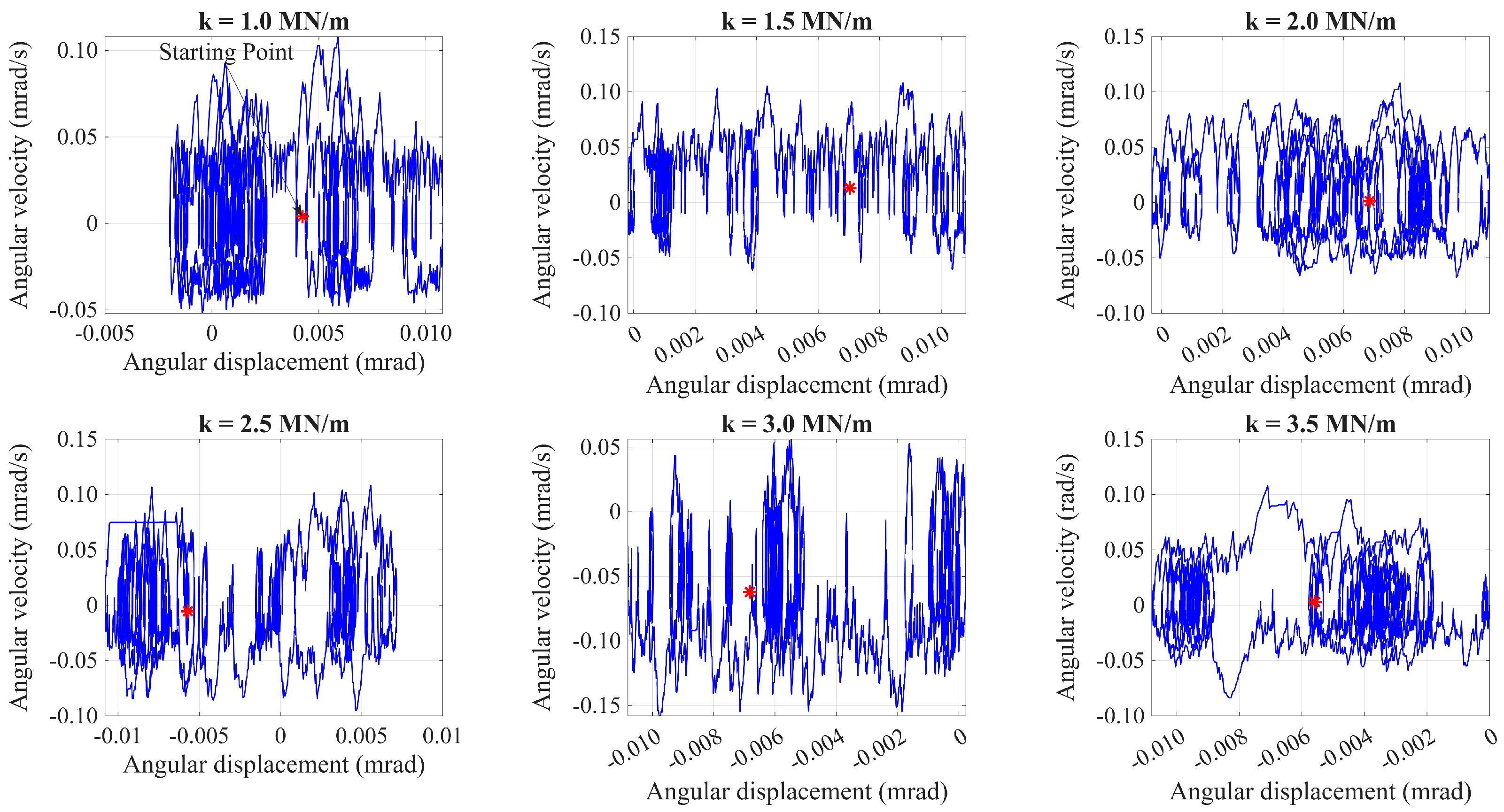
Figure 26 consists of six subplots corresponding to contact stiffness values of (a) $k=1.0\mathrm{MN}/\mathrm{m}$, (b) $1.5\mathrm{MN}/\mathrm{m}$, (c) $2.0\mathrm{MN}/\mathrm{m}$, (d) $2.5\mathrm{MN}/\mathrm{m}$, (e) $3.0\mathrm{MN}/\mathrm{m}$, and (f) $3.5\mathrm{MN}/\mathrm{m}$. Blue curves depict angular velocity versus angular displacement phase trajectories with red stars marking the initial state. At low stiffness ($1.0\mathrm{MN}/\mathrm{m}$), the trajectory exhibits large, irregular velocity spikes and a broad envelope, reflecting weak rebound, prolonged free flight, and chaotic stick–slip transitions. As stiffness increases to $1.5$–$2.0\mathrm{MN}/\mathrm{m}$, the envelope contracts with reduced velocity fluctuations; stronger rebounds shorten free-flight duration, yielding more periodic, stable stick–slip cycles. At $2.5$–$3.0\mathrm{MN}/\mathrm{m}$, sharp velocity spikes and defined loop structures emerge, indicating impulsive, high-intensity impacts with clear contact–free flight–impact transitions. At maximum stiffness ($3.5\mathrm{MN}/\mathrm{m}$), the trajectory becomes compact and highly periodic with small, well-defined loops; impacts are extremely brief and high-magnitude, effectively constraining motion to a near-continuous contact regime.

Contact stiffness thus governs energy transfer during impacts: low stiffness promotes chaotic, large-amplitude motion, while high stiffness drives the system toward stable, periodic behavior.

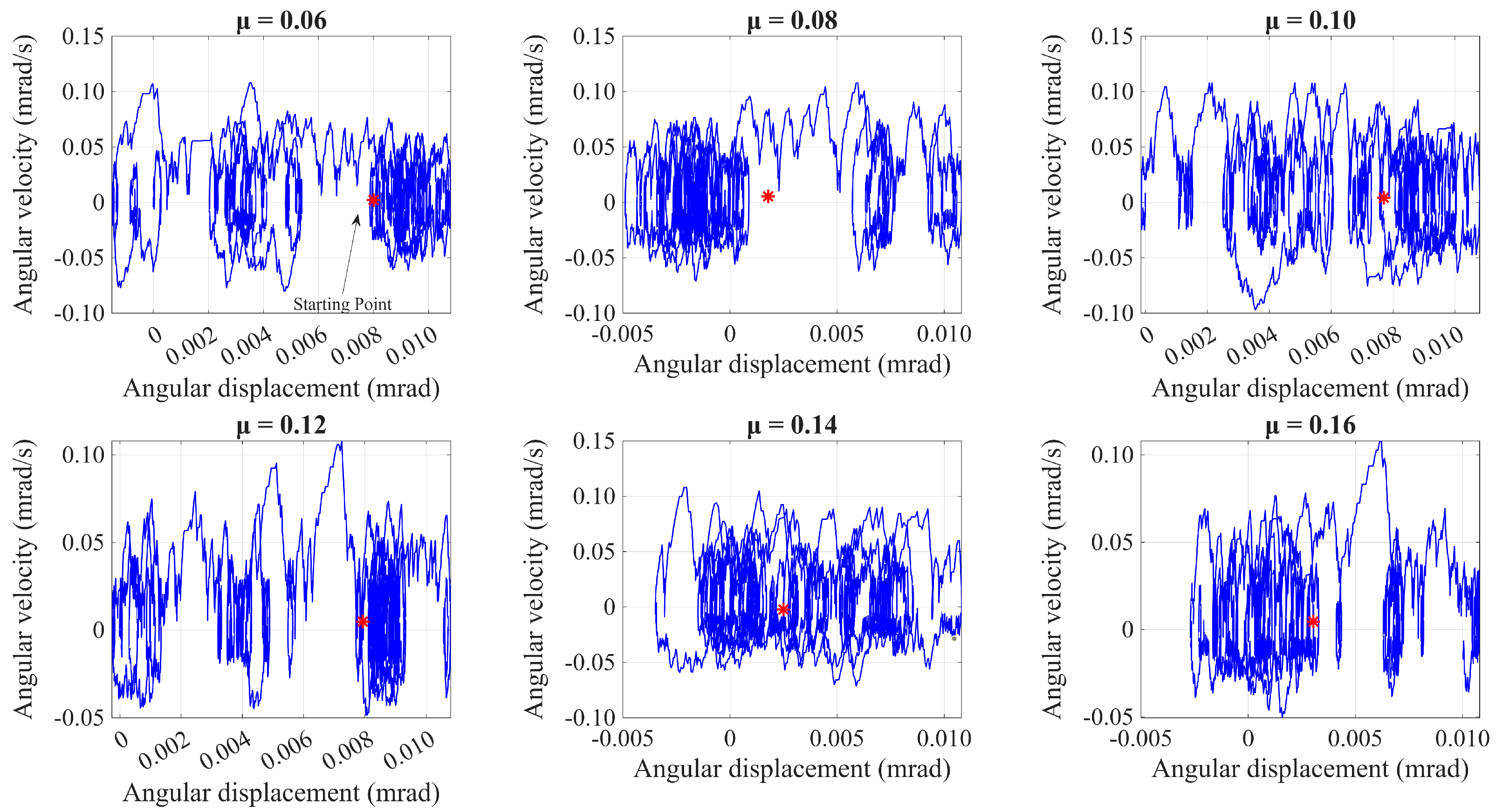
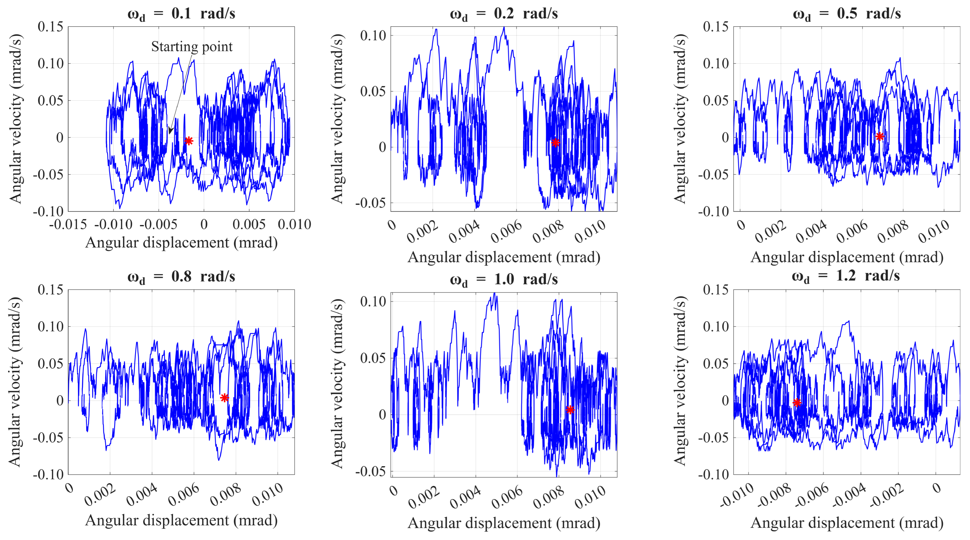
Figure 27 presents six phase portraits corresponding to friction coefficients of (a) $\mu =0.06$, (b) $0.08$, (c) $0.10$, (d) $0.12$, (e) $0.14$, and (f) $0.16$. Blue curves depict angular velocity versus angular displacement trajectories with red stars marking the initial state. At low friction ($\mu =0.06$), the trajectory is highly expanded and irregular with large velocity fluctuations, reflecting minimal damping, prolonged free flight, and chaotic slip-dominated motion. As friction increases to $0.08$–$0.10$, the envelope contracts with reduced velocity spikes; moderate damping balances stick and slip phases, yielding stable, repetitive stick–slip cycles. At $0.12$–$0.14$, sharper, more defined loops emerge with further reduced fluctuations, indicating constrained motion and stick-dominated behavior. At maximum friction ($\mu =0.16$), the trajectory becomes highly compact and near-periodic with minimal velocity variation; strong damping suppresses slip events, resulting in a near-continuous stick state and near-linear stable response.

Friction thus acts as a damping mechanism: low friction promotes chaotic, expanded trajectories, while high friction drives the system toward stable, periodic stick-dominated behavior.

4.3.4. Influence of Driving Force Frequency and Preload

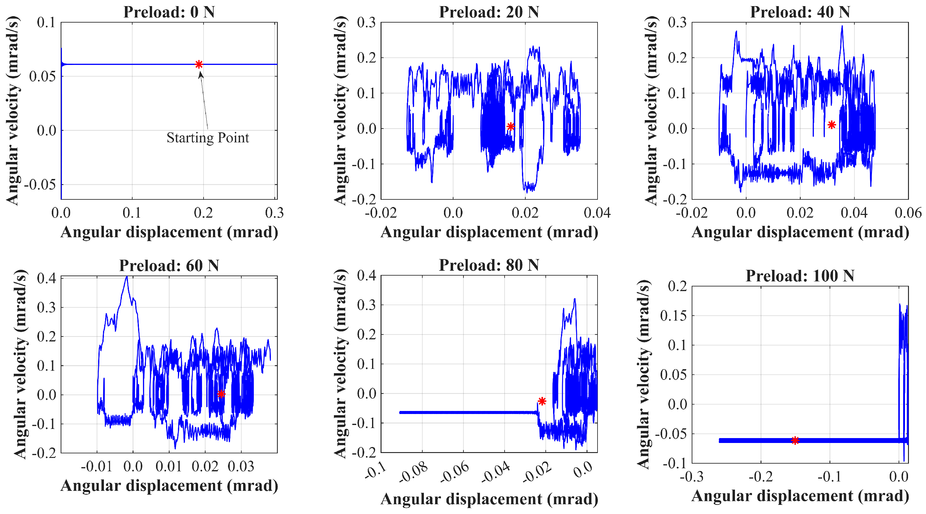
Figure 28 presents six phase portraits corresponding to preload forces of (a) $0\mathrm{N}$, (b) $20\mathrm{N}$, (c) $40\mathrm{N}$, (d) $60\mathrm{N}$, (e) $80\mathrm{N}$, and (f) $100\mathrm{N}$. Blue curves depict angular velocity versus angular displacement trajectories with red stars marking the initial state. At zero preload ($0\mathrm{N}$), the trajectory is a flat horizontal line, indicating pure inertial motion with no contact or friction. At low preload (20–$40\mathrm{N}$), the response becomes highly chaotic and expanded with large velocity fluctuations; weak contact pressure permits prolonged free flight and violent stick–slip impacts. At medium preload ($60\mathrm{N}$), the trajectory exhibits a mix of initial velocity spikes and subsequent compact loops, reflecting a partial suppression of free flight. At high preload (80–100 N), the trajectory contracts markedly with minimal velocity fluctuations; strong contact pressure effectively constrains the joint, resulting in near-static, stick-dominated behavior. At maximum preload ($100\mathrm{N}$), motion is nearly locked with only a brief terminal impact event.

Preload thus governs contact pressure and the degree of constraint: zero preload yields linear inertial motion, low preload induces chaotic impact-dominated dynamics, and high preload drives the system toward stable, constrained stick states.

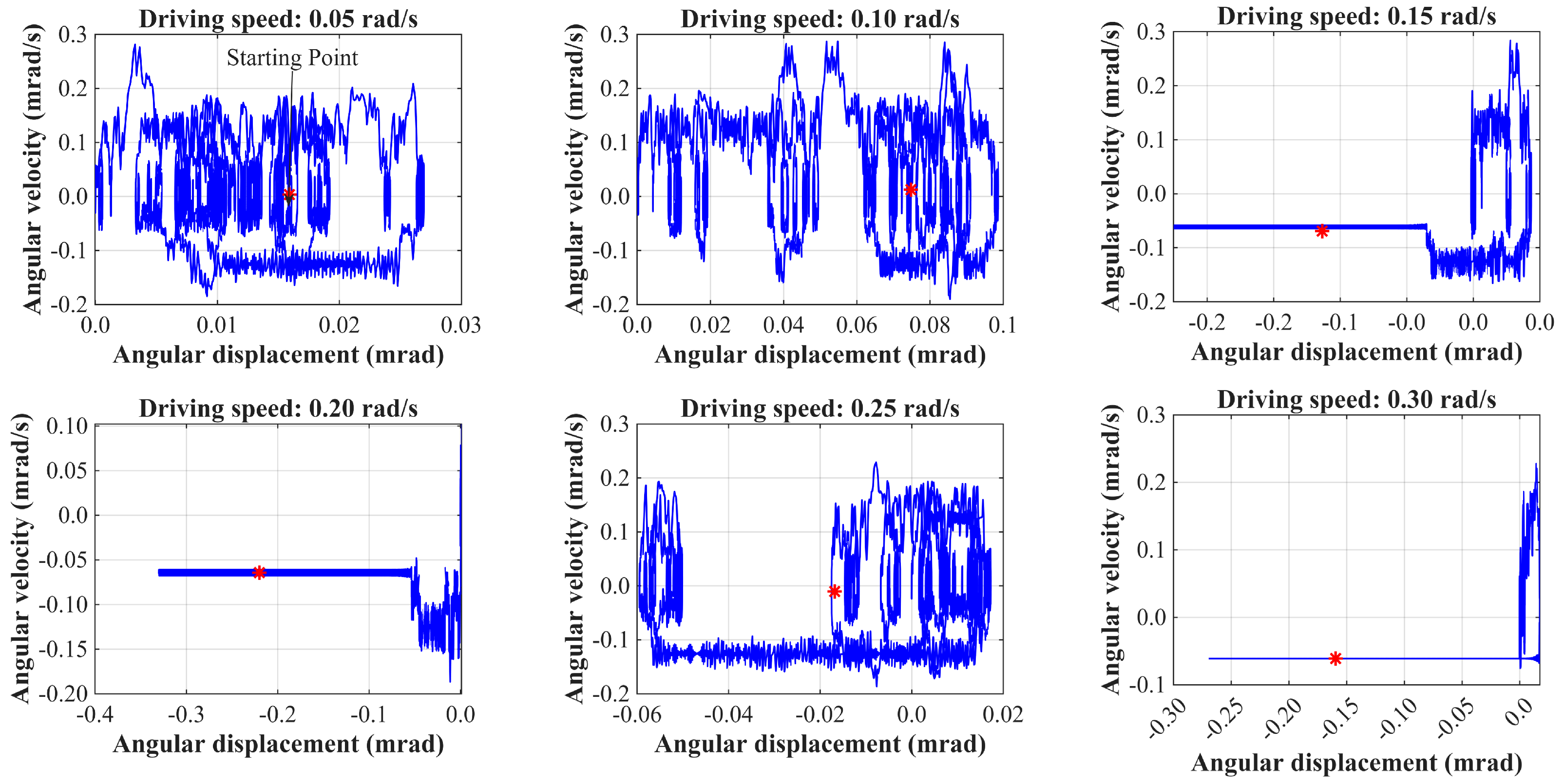
Figure 29 presents six phase portraits corresponding to driving angular velocities of (a) $0.05\mathrm{rad}/\mathrm{s}$, (b) $0.10\mathrm{rad}/\mathrm{s}$, (c) $0.15\mathrm{rad}/\mathrm{s}$, (d) $0.20\mathrm{rad}/\mathrm{s}$, (e) $0.25\mathrm{rad}/\mathrm{s}$, and (f) $0.30\mathrm{rad}/\mathrm{s}$. Blue curves depict angular velocity versus angular displacement trajectories with red stars marking the initial state. At low speed ($0.05\mathrm{rad}/\mathrm{s}$), the trajectory forms a compact, multi-looped cloud, reflecting prolonged contact and weak stick–slip cycles. As speed increases to $0.10$–$0.15\mathrm{rad}/\mathrm{s}$, the envelope expands with larger velocity spikes; higher inertial forces during free flight amplify impact intensity, and a distinct three-phase behavior (free flight, impact, contact) emerges. At $0.20\mathrm{rad}/\mathrm{s}$, a long flat free-flight segment dominates, culminating in a single terminal velocity spike, indicating near-inertial motion with minimal contact. At $0.25$–$0.30\mathrm{rad}/\mathrm{s}$, the response becomes chaotic and multi-looped again with repeated high-energy impacts and large velocity fluctuations driven by elevated inertial forces. Driving speed thus governs the balance between contact and free-flight phases: low speeds favor stick–slip-dominated periodic motion, intermediate speeds yield distinct free-flight and impact phases, and high speeds induce chaotic, impact-dominated dynamics.

Figure 30 presents six phase portraits corresponding to excitation frequencies of (a) ${\omega }_d=0.1\mathrm{rad}/\mathrm{s}$, (b) $0.2\mathrm{rad}/\mathrm{s}$, (c) $0.5\mathrm{rad}/\mathrm{s}$, (d) $0.8\mathrm{rad}/\mathrm{s}$, (e) $1.0\mathrm{rad}/\mathrm{s}$, and (f) $1.2\mathrm{rad}/\mathrm{s}$. Blue curves depict angular velocity versus angular displacement trajectories with red stars marking the initial state. At low frequency ($0.1\mathrm{rad}/\mathrm{s}$), the trajectory forms a compact, symmetric cloud with well-defined loops, reflecting weakly nonlinear, near-periodic stick–slip motion. As frequency increases to $0.2$–$0.5\mathrm{rad}/\mathrm{s}$, the envelope expands with larger velocity fluctuations; approaching resonance amplifies impact intensity and slip behavior, yielding moderately nonlinear, multi-looped responses. At resonance ($0.8\mathrm{rad}/\mathrm{s}$), the trajectory becomes highly chaotic and spread out with no clear periodicity, indicating maximized response and violent impact-dominated dynamics. Post-resonance ($1.0\mathrm{rad}/\mathrm{s}$), the trajectory contracts but remains irregular with residual nonlinearity. At high frequency ($1.2\mathrm{rad}/\mathrm{s}$), the response returns to a compact, near-periodic regime, as the system cannot fully follow rapid excitation. Excitation frequency thus governs response via resonance: near-natural frequencies amplify clearance-induced nonlinearity, producing chaotic, expanded trajectories, while off-resonance conditions suppress the response, yielding compact, weakly nonlinear stick–slip motion.

The parameter ranges used in this paper are strictly based on actual aerospace manufacturing standards and engineering practice. The radial clearance range of $0.01$–$0.1\mathrm{mm}$ corresponds to the typical radial clearance achievable with precision fits (e.g., H6/g5 to H8/f7) for hinge components in the 20–$50\mathrm{mm}$ nominal diameter range, covering tolerance grades IT5 to IT8 for the individual parts. The lower bound ($0.01\mathrm{mm}$) represents high-precision lapped fits used in ultra-stable pointing mechanisms, while the upper bound ($0.1\mathrm{mm}$) reflects the maximum acceptable clearance in large-scale deployable truss hinges.

Although the single-factor parametric analysis adopted here effectively isolates the individual influence of each parameter, real on-orbit conditions involve simultaneous multi-parameter interactions. The most significant coupling effects include temperature–clearance–friction coupling, clearance–driving speed–preload coupling, and thermal gradient–clearance coupling. These interactions can lead to dynamic behaviors that are not predictable by simple superposition of single-factor results. Future work will systematically investigate these coupling effects using design of experiments methods to develop comprehensive design guidelines for deployable antennas under extreme thermal environments.

5. Conclusions

A unified high-fidelity dynamic model based on the absolute nodal coordinate formulation is proposed for variable-geometry spacecraft deployable antennas with clearance hinges under extreme thermal environments. The proposed framework eliminates geometric nonlinear errors and mesh mismatch inherent in a conventional floating frame of reference formulation, enabling seamless multi-configuration deployment modeling without configuration switching while fully incorporating temperature-dependent material properties, thermal loads, and nonlinear clearance contact-friction characteristics. The model is established by deriving temperature-dependent mass, stiffness and damping matrices, formulating a nonlinear clearance contact force with temperature effects on contact stiffness and friction, and discretizing three typical deployment configurations (main boom translation, secondary arm rotation, and reflector deployment); the coupled thermo-mechanical governing equations are solved via an improved HHT-$\alpha$ implicit integration algorithm, and the model is validated against experimental data. Numerical results demonstrate that the proposed model achieves a calculation error below 2% versus experimental data, significantly outperforming the ABAQUS native classical Coulomb friction model (14.44–136.23% error); elevating the temperature from −200 °C to 200 °C reduces the first-order natural frequency by 10.8% and increases the thermally induced vibration amplitude by 120%; increasing the radial clearance from 0.01 mm to 0.1 mm amplifies the peak impact force by 211%; and a friction coefficient in the range of $0.08$–$0.10$ together with proper preload yields stable, repetitive stick–slip cycles and effectively mitigates chaotic nonlinear dynamics.

It should be noted that this paper focuses on revealing the fundamental thermo-mechanical coupling mechanism of clearance joints, and therefore, it adopts a simplified temperature field assumption considering only overall structural temperature rise and local frictional heating gradients. Future work will replace the current simplified uniform thermal boundary conditions with the practical external heat flux models developed by Fu et al. [46,47], which account for the temporal and spatial variations of Earth albedo, infrared radiation, and solar radiation along the orbit. This enhancement will enable an investigation of how non-uniform, time-varying thermal loads affect the temperature field distribution, thermally induced deformation patterns, and the stick–slip behavior of clearance hinges under more realistic on-orbit conditions.

References

1. Meguro, A.; Shintate, K.; Usui, M.; Tsujihata, A. In-orbit deployment characteristics of large deployable antenna reflector onboard Engineering Test Satellite VIII. Acta Astronaut. 2009, 65, 1306–1316. [Google Scholar] [CrossRef]
2. Zhang, X.; Nie, R.; Chen, Y.; He, B. Deployable Structures: Structural Design and Static/Dynamic Analysis. J. Elast. 2021, 146, 199–235. [Google Scholar] [CrossRef]
3. Tan, N.; Zhang, J.; Kazoleas, C.; Zhu, W.; Zhou, K.; Yuan, S. Dynamic modeling and vibrations of large deployable mesh reflectors. Appl. Math. Model. 2026, 150, 116329. [Google Scholar] [CrossRef]
4. Sun, J.; Jin, D.; Hu, H. Deployment dynamics and topology optimization of a spinning inflatable structure. Acta Mech. Sin. 2022, 38, 122100. [Google Scholar] [CrossRef]
5. Li, T.; Guo, J.; Cao, Y. Dynamic characteristics analysis of deployable space structures considering joint clearance. Acta Astronaut. 2011, 68, 974–983. [Google Scholar] [CrossRef]
6. Tian, Q.; Flores, P.; Lankarani, H.M. A comprehensive survey of the analytical, numerical and experimental methodologies for dynamics of multibody mechanical systems with clearance or imperfect joints. Mech. Mach. Theory 2018, 122, 1–57. [Google Scholar] [CrossRef]
7. Chen, Y.; Feng, J.; Peng, X.; Sun, Y.; He, Q.; Yu, C. An approach for dynamic analysis of planar multibody systems with revolute clearance joints. Eng. Comput. 2021, 37, 2159–2172. [Google Scholar] [CrossRef]
8. Guo, N.; Yun, W.; Zhang, S.; Du, H.; Xu, C. Finite Element Study on the Stiffness Variation Mechanisms of Radially Bolted Cylindrical-Cylindrical Shell Joints Under Transient Thermo-Mechanical Loading. Aerospace 2026, 13, 49. [Google Scholar] [CrossRef]
9. Polla, A.; Frulla, G.; Cestino, E.; Das, R.; Marzocca, P. Coupled thermo-mechanical numerical modeling of CFRP panel under high-velocity impact. Aerospace 2023, 10, 367. [Google Scholar] [CrossRef]
10. Kuang, Y.; Bai, Z.; Wei, C. Motion Accuracy and Dynamic Responses of Dual-Manipulator on Spacecraft Considering Clearance Joints. Aerospace 2026, 13, 75. [Google Scholar] [CrossRef]
11. Du, D.; Ma, S.; Zhang, Y.; Xu, K.; Lin, J.; Lv, S.; Sun, X.; Sun, W. Clearance Analysis of Rotor–Stator Coupled Structures Under Maneuver Flight Conditions Considering Multi-Physical Fields. Aerospace 2025, 12, 741. [Google Scholar] [CrossRef]
12. Mei, J.; Han, C.; Xu, Z.; Qi, Y.; Meng, Q.; Yang, Z.; Li, Z. Design, Analysis, and Experimentation of Space Deployable Segmented Solar Concentrator. Aerospace 2025, 12, 713. [Google Scholar] [CrossRef]
13. Wu, D.; Zhao, J.; Ma, X.; Chen, J.; Chen, C. Accuracy Analysis of a Multi-Closed-Loop Truss Antenna with Clearance. Aerospace 2024, 11, 1014. [Google Scholar] [CrossRef]
14. Thornton, E.A. Thermal Structures for Aerospace Applications; American Institute of Aeronautics and Astronautics: Reston, VA, USA, 1996. [Google Scholar] [CrossRef]
15. Boley, B.A. Thermally induced vibrations of beams. J. Aeronaut. Sci. 1956, 23, 179–181. [Google Scholar] [CrossRef]
16. Cao, Y.; Cao, D.; He, G.; Liu, L. Thermal alternation induced vibration analysis of spacecraft with lateral solar arrays in orbit. Appl. Math. Model. 2020, 86, 166–184. [Google Scholar] [CrossRef]
17. Shen, Z.; Li, H.; Liu, X.; Hu, G. Thermal-structural dynamic analysis of a satellite antenna with the cable-network and hoop-truss supports. J. Therm. Stress. 2019, 42, 1339–1356. [Google Scholar] [CrossRef]
18. Shen, Z.; Tian, Q.; Liu, X.; Hu, G. Thermally induced vibrations of flexible beams using Absolute Nodal Coordinate Formulation. Aerosp. Sci. Technol. 2013, 29, 386–393. [Google Scholar] [CrossRef]
19. Cui, Y.; Yu, Z.; Lan, P. A novel method of thermo-mechanical coupled analysis based on the unified description. Mech. Mach. Theory 2019, 134, 376–392. [Google Scholar] [CrossRef]
20. Obrezkov, L.P.; Mikkola, A.; Matikainen, M.K. Performance review of locking alleviation methods for continuum ANCF beam elements. Nonlinear Dyn. 2022, 109, 531–546. [Google Scholar] [CrossRef]
21. Tian, Q.; Yu, Z.; Lan, P.; Cui, Y.; Lu, N. Model order reduction of thermo-mechanical coupling flexible multibody dynamics via free-interface component mode synthesis method. Mech. Mach. Theory 2022, 172, 104786. [Google Scholar] [CrossRef]
22. Yu, Z.; Cui, Y.; Zhang, Q.; Liu, J.; Qin, Y. Thermo-mechanical coupled analysis of V-belt drive system via absolute nodal coordinate formulation. Mech. Mach. Theory 2022, 174, 104906. [Google Scholar] [CrossRef]
23. Tian, Q.; Sun, H.; Yu, Z. Model order reduction of thermal-dynamic coupled flexible multibody system with multiple varying parameters. Appl. Math. Model. 2024, 136, 115634. [Google Scholar] [CrossRef]
24. Abdalla, M.; Elbakly, M.; Shabana, A.A. Computational algorithm for the solution of coupled thermomechanical large-displacement problems. Acta Mech. 2025. [Google Scholar] [CrossRef]
25. Yuan, T.; Lei, B.; Liu, J.; Wu, Y. Rigid–flexible–thermal coupling dynamics of a hub and multiplate system considering frictional contact. Multibody Syst. Dyn. 2023, 59, 363–394. [Google Scholar] [CrossRef]
26. Zhou, Z.; Xu, Y. Thermo-flexible coupled dynamics of composite laminated plates based on absolute nodal coordinate formulation. Mech. Adv. Mater. Struct. 2025, 32, 4673–4689. [Google Scholar] [CrossRef]
27. Sun, X.; Jin, J.; Chen, Z. Thermo-flexible coupled modeling and active control of thermally induced vibrations for a flexible plate. Thin-Walled Struct. 2025, 211, 113092. [Google Scholar] [CrossRef]
28. Li, C.; Tao, J.; Xiao, H.; Zhao, R.; Xing, S.; Guo, H.; Jiang, Y.; Xu, J.; Zhu, G.; Yang, G. Thermoelastic dynamic model for a telescopic wing system based on an absolute nodal coordinate formulation deployable thin plate element. Thin-Walled Struct. 2025, 214, 113372. [Google Scholar] [CrossRef]
29. Zhou, Z.; Xu, Y.; Cao, C.; Sheng, X. Dynamics for rigid-flexible-thermal coupled solar panel multibody system composed of composite laminated shells. Mech. Based Des. Struct. Mach. 2025, 53, 7382–7407. [Google Scholar] [CrossRef]
30. Ma, Z.; Shen, Z.; Wu, M.; Wang, Y. Thermally induced vibrations of thin-walled composite circular tubes on spacecraft via higher-order ANCF beam elements. Compos. Struct. 2026, 379, 119979. [Google Scholar] [CrossRef]
31. Armanini, C.; Boyer, F.; Mathew, A.T.; Duriez, C.; Renda, F. Soft Robots Modeling: A Structured Overview. IEEE Trans. Robot. 2023, 39, 1728–1748. [Google Scholar] [CrossRef]
32. Li, Y.; Wang, C.; Huang, W. Rigid-flexible-thermal analysis of planar composite solar array with clearance joint considering torsional spring, latch mechanism and attitude controller. Nonlinear Dyn. 2019, 96, 2031–2053. [Google Scholar] [CrossRef]
33. Jin, L.; Zhang, F.; Tian, D.; Wang, Q.; Cao, Q. Thermal-Structural Analysis of the Support Structure for a Modular Space Deployable Antenna. Int. J. Aerosp. Eng. 2022, 2022, 2164485. [Google Scholar] [CrossRef]
34. Lankarani, H.M.; Nikravesh, P.E. A Contact Force Model with Hysteresis Damping for Impact Analysis of Multibody Systems. In Proceedings of the ASME 1989 International Design Engineering Technical Conferences and Computers and Information in Engineering Conference, Anaheim, CA, USA, 30 July–3 August 1989; pp. 45–51. [Google Scholar] [CrossRef]
35. Flores, P. Concepts and Formulations for Spatial Multibody Dynamics; Springer International Publishing: Cham, Switzerland, 2015. [Google Scholar] [CrossRef]
36. Shabana, A.A. Dynamics of Multibody Systems; Cambridge University Press: New York, NY, USA, 2020. [Google Scholar] [CrossRef]
37. Shabana, A.A. Computational Continuum Mechanics; John Wiley & Sons: Hoboken, NJ, USA, 2018. [Google Scholar] [CrossRef]
38. Gerstmayr, J.; Sugiyama, H.; Mikkola, A. Review on the absolute nodal coordinate formulation for large deformation analysis of multibody systems. J. Comput. Nonlinear Dyn. 2013, 8, 031016. [Google Scholar] [CrossRef]
39. Flores, P.; Koshy, C.S.; Lankarani, H.M.; Ambr’osio, J.A.C.; Claro, J.C.P. Numerical and experimental investigation on multibody systems with revolute clearance joints. Nonlinear Dyn. 2011, 65, 383–398. [Google Scholar] [CrossRef]
40. Wilson, S.; Alpas, A.T. Effect of temperature on the sliding wear performance of Al alloys and Al matrix composites. Wear 1996, 196, 270–278. [Google Scholar] [CrossRef]
41. Shimizu, S.; Ishimura, K.; Miyashita, T.; Parque, V. Structural analysis of thermally induced stick-slip on deployable mast. In Proceedings of the AIAA Scitech 2019 Forum, San Diego, CA, USA, 7–11 January 2019. [Google Scholar] [CrossRef]
42. Shen, Y.; Wang, C.; Hua, Y.; Tan, S.; Zheng, Q.; Gao, J. Dynamic analysis and driving parameters study of bidirectional solar array system with multiple clearance joints. Meccanica 2025, 60, 953–972. [Google Scholar] [CrossRef]
43. Shen, Y.; Wang, C.; Tan, S.; Hua, Y.; Gao, J. Dynamic Modeling and Synchronous Deployment Analysis of Bidirectional Solar Array with Clearances. Aiaa J. 2025, 63, 5001–5012. [Google Scholar] [CrossRef]
44. Zhang, S.; Zhao, D. (Eds.) Aerospace Materials Handbook, 1st ed.; CRC Press: Boca Raton, FL, USA, 2016. [Google Scholar] [CrossRef]
45. Blythe, M.P.; Saunders, M.P.; Pye, D.B.; Voss, L.D.; Moreland, R.J.; Symon, K.E.; Bromley, L.K. NASA Space Flight Program and Project Management Handbook; NASA Special Publication NASA/SP-2014-3705; National Aeronautics and Space Administration: Washington, DC, USA; 12th Media Services: Suwanee, GA, USA, 2014.
46. Fu, X.; Hua, Y.; Ma, W.; Cui, H.; Zhao, Y. An Innovative External Heat Flow Expansion Formula for Efficient Uncertainty Analysis in Spacecraft Earth Radiation Heat Flow Calculations. Aerospace 2023, 10, 605. [Google Scholar] [CrossRef]
47. Fu, X.; Hua, Y.; Ma, W.; Cui, H.; Zhao, Y. Novel heat flux expansion formula for spacecraft solar radiation uncertainty analysis. Numer. Heat Transf. Part A 2025, 86, 2596–2617. [Google Scholar] [CrossRef]
Figure 1. Schematic flowchart illustrating the complete workflow for constructing thermo-mechanical coupling matrices using the ANCF.
Aerospace 13 00529 g001
Figure 2. Schematic of ANCF elements: 4-node 3D thick cylindrical shell element for main boom and secondary arm.
Aerospace 13 00529 g002
Figure 3. Schematic of ANCF elements: 2-node 3D thin-walled curved beam element for ring truss reflector.
Aerospace 13 00529 g003
Figure 4. Schematic of the revolute clearance hinge contact model: Basic geometric parameter definition.
Aerospace 13 00529 g004
Figure 5. Motion states and contact mechanics model with thermo-mechanical coupling effects. The arrow in the figure indicates heat generated by friction.
Aerospace 13 00529 g005
Figure 6. Workflow of the improved HHT- α time integration scheme for thermal–structural coupled dynamics with contact friction and stick–slip effects.
Aerospace 13 00529 g006
Figure 7. Schematic of three typical kinematic pairs in the deployable antenna mechanism.
Aerospace 13 00529 g007
Figure 8. Geometric configuration and degree of freedom (DOF) definition of the antenna deployment joint.
Aerospace 13 00529 g008
Figure 9. ANCF finite element meshing of the deployment joint for degeneration validation.
Aerospace 13 00529 g009
Figure 10. Thermally induced rotational response of triangular hinge under uniform temperature rise ( Δ T = 55   ° C , Δ T = 105   ° C , Δ T = 155   ° C ).
Aerospace 13 00529 g010
Figure 11. Thermally induced rotational response of the pentagonal hinge under graded axial temperature gradients ( 5   ° C / mm , 10   ° C / mm , 15   ° C / mm ).
Aerospace 13 00529 g011
Figure 12. Normalized dynamic response amplitude of the deployable mechanism with different clearance joint types and sizes under varying excitation frequencies.
Aerospace 13 00529 g012
Figure 13. Finite element model of the ASTRO-H imitating deployable mast for full model validation and structural schematic of the benchmark experimental prototype.
Aerospace 13 00529 g013
Figure 14. Spatial configuration and contact collision state of the main boom–secondary arm system at the final deployment stage (Configuration 1 with preload).
Aerospace 13 00529 g014
Figure 15. Spatial configuration and contact collision state of the main boom–secondary arm system at the final deployment stage (Configuration 1 without preload).
Aerospace 13 00529 g015
Figure 16. Thermal slip–stick state distribution on the contact surfaces of the main boom translation joint (Configuration 1).
Aerospace 13 00529 g016
Figure 17. Four-stage spatial configuration evolution of the secondary arm during rotational deployment (configuration 2: rotational deployment).
Aerospace 13 00529 g017
Figure 18. Spatiotemporal distribution of thermal deformation and stick–slip state of the clearance joint (Configuration 2: rotational deployment).
Aerospace 13 00529 g018
Figure 19. Deployment sequence of the ring truss antenna at key stages (Configuration 3: antenna deployment).
Aerospace 13 00529 g019
Figure 20. Node trajectory and thermal deformation of the ring truss antenna at key nodes under orbital thermal loads (Configuration 3: antenna deployment).
Aerospace 13 00529 g020
Figure 21. Time response and phase space trajectory of the ring truss antenna joint under thermo-clearance coupling excitation.
Aerospace 13 00529 g021
Figure 22. Phase portraits of joint angular velocity under transient temperature conditions ( 19.85 169.85   ° C ).
Aerospace 13 00529 g022
Figure 23. Phase portraits of joint angular velocity under initial temperature conditions ( T = 150   ° C to 100   ° C ).
Aerospace 13 00529 g023
Figure 24. Phase portraits of joint angular velocity under different radial clearances ( 0.02 0.14 mm ).
Aerospace 13 00529 g024
Figure 25. Phase portraits of joint angular velocity under different radial clearances ( c = 0.002 0.012 mm ).
Aerospace 13 00529 g025
Figure 26. Phase portraits of joint angular velocity under different contact stiffness values ( k = 1.0 3.5 MN / m ).
Aerospace 13 00529 g026
Figure 27. Phase portraits of joint angular velocity under different friction coefficients ( μ = 0.06 0.16 ).
Aerospace 13 00529 g027
Figure 28. Phase portraits of joint angular velocity under different preload levels (0–100 N).
Aerospace 13 00529 g028
Figure 29. Phase portraits of joint angular velocity under different driving speeds ( 0.05 0.30 rad / s ).
Aerospace 13 00529 g029
Figure 30. Phase portraits of joint angular velocity under different driving frequencies ( ω d = 0.1 1.2 rad / s ).
Aerospace 13 00529 g030