Robust Model Predictive Control for Autonomous Spacecraft Close-Proximity Operations Around an Asteroid

Abstract

To address the robustness of autonomous proximity trajectories in asteroid exploration missions under model uncertainties and external disturbances, this paper proposes a tube-based model predictive control (TBMPC) framework with disturbance identification for a six-degree-of-freedom nonlinear model. Specifically, the inner layer employs a sequential convex optimization-based nonlinear MPC framework to solve the nominal trajectory optimization problem, while the outer layer dynamically estimates the disturbance set using real-time measurement information through an online exogenous input identification mechanism and adaptively adjusts the size of the disturbance-invariant tube, thereby effectively reducing the conservatism caused by the fixed disturbance bounds in conventional TBMPC. In addition, a sensitivity analysis of the forgetting factor parameter is conducted to investigate the influence of different forgetting factor values on system performance. Finally, 100 Monte Carlo simulations are performed to further verify the robustness and stability of the proposed method under randomly bounded disturbances. The results show that all actual trajectories remain within the disturbance-invariant tube, demonstrating the good engineering applicability of the proposed method.

1. Introduction

With the continuous advancement of deep-space exploration missions, asteroid exploration has become an important research direction in the aerospace field. Typical mission scenarios include close-proximity flybys and autonomous landings [1,2], which impose stringent requirements on the orbit and attitude control of spacecraft. However, asteroids are usually characterized by irregular shapes, non-uniform mass distributions, and weak gravitational fields, leading to highly complex gravitational environments. In addition, there exist other external disturbances that are difficult to model accurately. These factors significantly increase the uncertainty in orbital dynamics. In this paper, asteroid gravity modeling errors, actuator uncertainties, linearization errors, and other unmodeled dynamics are modeled as bounded disturbances.

Traditional deterministic trajectory planning and control methods [3,4,5,6,7] typically rely on precise models, making it difficult to guarantee constraint satisfaction and system stability in the presence of uncertainties and external disturbances. At present, numerous methods have been developed for uncertainty propagation analysis, primarily applied in tasks such as orbit determination and space situational awareness. For uncertainties assumed to follow Gaussian distributions, the evolution of the mean and covariance [8] is typically analyzed. In contrast, the state transition tensor (STT) [9] and polynomial chaos expansion [10] techniques are commonly employed to characterize the propagation of non-Gaussian uncertainties. Directional state transition tensor (DSTT) [11] and time-varying DSTT (TDSTT) [12] are proposed to improve the computational efficiency of STT. The high-order extended Kalman filter based on differential algebra [13] achieves accuracy comparable to the STT method, but its computational efficiency is much higher than that of the traditional STT method.

Although robust control methods can enhance the system’s ability to handle uncertainties to some extent, they often suffer from excessive conservatism or difficulties in handling state constraints. Model predictive control (MPC) [14,15,16,17], due to its capability of explicitly handling multi-constraint optimization problems, has been widely applied in spacecraft trajectory planning and tracking control. Data-driven approaches [18] have significantly expanded the applicability of MPC by reducing reliance on accurate first-principles models and enabling control design directly from data. For linear parameter-varying (LPV) systems, an optimization-based constraint tightening method [19] is proposed to enhance the robustness of model predictive control and ensure constraint satisfaction in the presence of uncertainties. For the soft landing on an asteroid surface, an input observer is incorporated into the MPC optimization framework [20] to compensate for the mismatch between the gravity model and the asteroid’s actual gravitational field, thereby improving positioning accuracy.

However, standard MPC cannot directly guarantee robust constraint satisfaction in the presence of bounded disturbances. To address this issue, tube-based model predictive control (TBMPC) [21,22,23] constrains the actual system state within a “tube” around the nominal trajectory by constructing a robust positively invariant set of the error system, thereby achieving robustness against bounded disturbances. Lishkova [24] proposed a robust receding horizon control method for convex dynamical systems with bounded disturbances, which explicitly accounts for disturbances in the prediction and constructs constraint-satisfying control laws, thereby ensuring robust feasibility and closed-loop stability. Mammarella et al. [25] developed a tube-based robust model predictive control strategy for spacecraft proximity operations under persistent disturbances by confining the actual trajectory within a robust invariant tube around a nominal trajectory to ensure constraint satisfaction and robust stability. Rakovi [26] proposed an implicit rigid tube model predictive control method, which avoids explicitly constructing the tube set to reduce computational complexity.

However, conventional tube MPC typically relies on a pre-designed fixed tube set, which remains unchanged during operation. This offline design heavily depends on the estimation of disturbance bounds: if the initial estimate is too small, the actual disturbance may exceed the tube, leading to degraded robustness or even constraint violation; if it is too large, excessive conservatism is introduced, resulting in degraded control performance. To overcome these limitations, this paper introduces a forgetting factor method into the TBMPC framework to enable online weighted updating of disturbance information, thereby achieving adaptive adjustment of the tube set. By dynamically estimating the disturbance bounds and adjusting the size of the robust positively invariant set online, the proposed method not only guarantees system robustness but also effectively alleviates the conservatism caused by fixed tubes, improving adaptability to time-varying disturbance environments. Lopez [27] proposed an adaptive dynamic tube MPC, which employs set membership identification to online estimate the bounded external disturbance set and dynamically adjust the robust tube, achieving adaptive control, robust constraint satisfaction, and performance optimization for nonlinear systems under uncertainties and disturbances. Oestreich [28] combined the forgetting factor with an ARMA identification model to estimate external inputs and uncertainties in the target’s inertia tensor. Jiang [29] achieved path-tracking control for high-speed intelligent vehicles by adaptively adjusting the prediction horizon and control horizon. An asynchronous computation framework for tube-based model predictive control [30] is proposed, which decouples the optimization process from system evolution, thereby reducing computational burden while ensuring robustness and constraint satisfaction.

Current tube model predictive control (tube MPC) research mainly focuses on linear systems with bounded disturbances. Existing studies on nonlinear systems are typically limited to simplified translational dynamics, while applications to six-degree-of-freedom (6-DOF) nonlinear coupled translational–attitudinal systems remain scarce due to the high computational complexity of the resulting optimization problem. In asteroid exploration scenarios, spacecraft are subject to significant environmental disturbances in microgravity, making the design of safe and robust proximity trajectories essential. Tube MPC ensures robust constraint satisfaction by constructing a disturbance set and an associated invariant tube that bounds the actual system trajectory under disturbances.

The disturbance set update strategy adopted in this paper is based on the method proposed in Reference [28], which considers a 3-DOF linear double-integrator system. In contrast, this work extends the approach to a 6-DOF nonlinear coupled translational–attitudinal dynamics model for asteroid exploration scenarios, while incorporating complex constraints such as approach cone constraints and line-of-sight angle constraints.

6-DOF coupled translational–attitudinal dynamics models are typically highly nonlinear and high-dimensional, making the associated optimal control problem computationally challenging. To address this issue, sequential convex optimization schemes are commonly employed, where the nonlinear model is approximated and solved iteratively using efficient solvers such as interior-point methods. However, in practice, issues such as artificial infeasibility may arise, or the linearization process may lead to an unbounded optimization problem. To mitigate these issues, virtual control inputs, slack variables, or trust-region constraints [31] are often introduced to improve feasibility and enhance numerical stability.

Therefore, the main contribution of this work lies in the integration and application of an existing disturbance-identification-based tube MPC approach for a complex 6-DOF asteroid proximity tracking problem, thereby improving trajectory-tracking robustness and safety in uncertain dynamical environments.

2. Materials and Methods

2.1. Dynamic Model

The orbital dynamics of the asteroid exploration mission are modeled as a restricted three-body problem [32], while the attitude is represented using the projection of quaternions onto their tangent space. First, three coordinate frames are defined:

• Inertial frame I: The origin is located at the asteroid’s center of mass, and its three axes are fixed in inertial space;
• Orbital frame L: The origin is also located at the asteroid’s center of mass; the x-axis points from the Sun to the asteroid, the z-axis is parallel to the normal direction of the asteroid’s orbital plane, and the y-axis is determined according to the right-hand rule;
• Spacecraft body frame B: The origin is located at the spacecraft’s center of mass, and its axes are aligned with the spacecraft’s principal axes of inertia.
• Asteroid body frame A: The origin is located at the asteroid’s mass center, with axes aligning to the principal axes of inertia of the asteroid.

Due to the highly irregular shape of asteroids, it is difficult to accurately model their gravitational field using a point mass gravity model. Therefore, a polyhedral model is adopted in this paper to characterize the gravitational field [33]. In addition, solar radiation pressure and third-body gravitational effects are taken into account. The resulting orbital dynamics model is given by

$$\ddot{\mathit{r}}=-2n\widehat{\mathit{z}}\times \dot{\mathit{r}}+n^2(3\widehat{\mathit{x}}{\widehat{\mathit{x}}}^T-\widehat{\mathit{z}}{\widehat{\mathit{z}}}^T)·\mathit{r}+{\displaystyle \frac{{\beta }_{\mathrm{SRP}}}{R^2}}\widehat{\mathit{x}}+\nabla U^L+{\mathit{u}}_{\mathit{p}}$$

(1)

$n=\sqrt{{\mu }_{\mathrm{sun}}/R^3}$ denotes the mean orbital angular velocity of the small body in its heliocentric orbit, where R is the semi-major axis of the heliocentric orbit. $\widehat{\mathit{x}}$ and $\widehat{\mathit{z}}$ are unit vectors along the x-axis and z-axis of the orbital frame, respectively. ${\mu }_{\mathrm{sun}}$ is the gravitational constant of the Sun. ${\beta }_{\mathrm{SRP}}$ is defined as ${\beta }_{\mathrm{SRP}}={\displaystyle \frac{P_0\left(1+\rho \right){\left(1\mathrm{AU}\right)}^{2}A}{m}}$. $A/m$ is the effective area-to-mass ratio of the spacecraft. $\rho$ is the albedo of the asteroid. The gravitational gradient is typically expressed in the asteroid body frame A, and its specific expression is given as follows:

$$\nabla U^A=-G_g\rho \sum _{e\in edges}{E}_e{r}_e{L}_e+G_g\rho \sum _{f inf aces}{F}_f{r}_f{\Omega }_f$$

(2)

where $G_g$ is the universal gravitational constant, and $\rho$ is the density of the asteroid. The specific calculations for each term are presented in [34]. In the equation, $r_e$ and $r_f$ denote the relative distances from the spacecraft to the edge and surface of the asteroid, respectively. Since the spacecraft position is expressed in the orbital frame L, a coordinate transformation is required as follows:

$$r^A=q_{A/L}\odot r^L\odot q_{A/L}^{*}$$

(3)

$$\nabla U^L=q_{A/L}\odot \nabla U^A\odot q_{A/L}^{*}$$

(4)

where $q_{A/L}$ denotes the rotation quaternion from the orbital frame L to the asteroid body frame A. Since both the asteroid’s rotation rate ${\omega }_A$ and the heliocentric orbital frame angular velocity ${\omega }_L$ are constant, the corresponding quaternion at each time instant can be obtained by the following integration:

$${\dot{\mathit{q}}}_{\mathrm{L}/\mathrm{I}}={\displaystyle \frac{1}{2}}{\omega }_{\mathrm{L}/\mathrm{I}}^{\mathrm{L}}\odot {\mathit{q}}_{\mathrm{L}/\mathrm{I}}$$

(5)

$${\dot{\mathit{q}}}_{\mathrm{A}/\mathrm{I}}={\displaystyle \frac{1}{2}}{\omega }_{\mathrm{A}/\mathrm{I}}^{\mathrm{A}}\odot {\mathit{q}}_{\mathrm{A}/\mathrm{I}}$$

(6)

The transformation from the orbital frame L to the body frame A is

$${\mathit{q}}_{\mathrm{A}/\mathrm{L}}={\mathit{q}}_{A/I}\odot {\mathit{q}}_{L/I}^{*}$$

(7)

By integrating Equation (7), $q_{A/L}$ at each time instant can be obtained. Substituting it into Equation (3) yields the relative position in the asteroid body frame. This result is then further substituted into Equation (2) and subsequently Equation (4), allowing the gravity gradient expressed in the orbital frame to be obtained. ⊗ and ⊙ denote quaternion multiplication operators. For two quaternions $\mathit{p}=[\mathit{p},p_0]$ and $\mathit{q}=[\mathit{q},q_0]$, these operators are defined as follows:

$$\mathit{q}\otimes \mathit{p}=\left[\begin{array}{c}{p}_0\mathit{q}+q_0\mathit{p}+\mathit{q}\times \mathit{p}\\ q_0{p}_0-{\mathit{q}}^T\mathit{p}\end{array}\right]\mathit{q}\odot \mathit{p}=\left[\begin{array}{c}{p}_0\mathit{q}+q_0\mathit{p}-\mathit{q}\times \mathit{p}\\ q_0{p}_0-{\mathit{q}}^T\mathit{p}\end{array}\right]$$

(8)

The attitude dynamics of the body frame with respect to the orbital frame can be expressed as

$${\dot{\omega }}_{\mathrm{B}/\mathrm{L}}^{\mathrm{B}}=J^{-1}\left({\mathit{T}}^B-\left({\omega }_{\mathrm{B}/\mathrm{L}}^{\mathrm{B}}+{\omega }_{\mathrm{L}/\mathrm{I}}^{\mathrm{B}}\right)\times J\left({\omega }_{\mathrm{B}/\mathrm{L}}^{\mathrm{B}}+{\omega }_{\mathrm{L}/\mathrm{I}}^{\mathrm{B}}\right)\right)+{\omega }_{\mathrm{B}/\mathrm{L}}^{\mathrm{B}}\times {\omega }_{\mathrm{L}/\mathrm{I}}^{\mathrm{B}}$$

(9)

$${\dot{\mathit{q}}}_{\mathrm{B}/\mathrm{L}}={\displaystyle \frac{1}{2}}{\omega }_{\mathrm{B}/\mathrm{L}}^{\mathrm{B}}\odot {\mathit{q}}_{\mathrm{B}/\mathrm{L}}$$

(10)

To facilitate the handling of additive disturbances, this paper employs the exponential map ${\mathit{q}}_{\mathrm{B}/\mathrm{L}}=e^{{\displaystyle \frac{\varphi }{2}}}$ to establish the relationship between the tangent space, i.e., the Lie algebra, and the rotation space represented by unit quaternions. The tangent space essentially corresponds to the Lie algebra of the unit quaternion sphere, providing a natural linear space for handling additive disturbances while maintaining a strict correspondence with the original quaternion rotation. By applying the logarithmic map and differentiating the Lie algebra, we obtain

$$\dot{\mathit{\varphi }}=2{\mathit{q}}_{\mathrm{B}/\mathrm{L}}^{-1}\otimes {\displaystyle \frac{1}{2}}{\mathit{q}}_{\mathrm{B}/\mathrm{L}}\otimes {\mathit{\omega }}_{\mathrm{B}/\mathrm{L}}^{\mathrm{B}}={\mathit{\omega }}_{\mathrm{B}/\mathrm{L}}^{\mathrm{B}}$$

(11)

From the above equation, it can be seen that the derivative of the Lie algebra depends solely on the angular velocity. Compared to other attitude representations, this greatly simplifies the kinematic formulation.

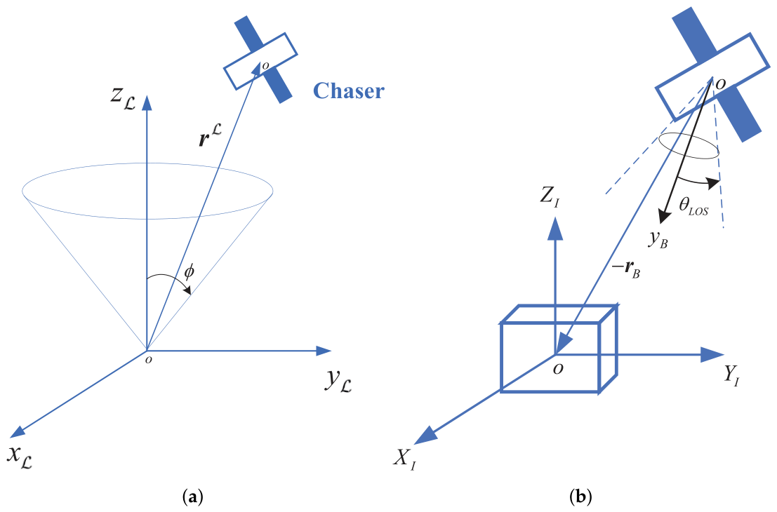
To ensure that the spacecraft does not collide with the asteroid upon reaching the target point during the proximity operation while simultaneously maintaining the target within the line of sight, this paper introduces a glide-slope constraint and an attitude–orbit coupled line-of-sight (LOS) constraint, as shown in Figure 1. The glide-slope constraint is defined in the orbital frame, and the formulation is given as follows:

$${\mathit{r}}_L·{\widehat{\mathit{z}}}_L\ge \parallel {\mathit{r}}_L\parallel cos\varphi$$

(12)

Here, $\varphi$ denotes the half-cone angle, and ${\mathit{z}}_L$ is the unit vector along the z-axis of the orbital frame. The LOS constraint, on the other hand, is defined in the body frame:

$$-{\mathit{r}}_B·{\mathit{y}}_B\ge \parallel {\mathit{r}}_B\parallel cos{\theta }_{LOS}$$

(13)

This constraint can be formulated as a conical region with a half-angle ${\theta }_{LOS}$ about the optical-axis ${\mathit{y}}_B$ direction in the body-fixed coordinate frame B.

The coupled dynamics are considered to properly capture the interaction between translational and rotational motions, which is essential for enforcing line-of-sight and attitude-pointing constraints during proximity operations. However, the proposed framework does not involve onboard navigation or orbit determination, and the system state is assumed to be available from an external estimator. Therefore, this study should be regarded as a tracking control framework rather than a full autonomous navigation and control system.

2.2. Tube-Based Model Predictive Control Framework

2.2.1. Standard Tube-Based Model Predictive Control

Tube-based model predictive control (TBMPC) is an effective control strategy for guaranteeing constraint satisfaction in the presence of system uncertainties. Regardless of whether open-loop control or closed-loop feedback control is employed, uncertainties give rise to a corresponding tube set during the system evolution. Although uncertainties evolve over time and continuously affect the system dynamics, the constructed tube ensures that the actual system state remains confined within it.

A linear discrete-time nominal system:

$${\mathit{z}}_{\mathit{k}+\mathit{1}}=\mathit{A}{\mathit{z}}_{\mathit{k}}+\mathit{B}{\mathit{v}}_{\mathit{k}},k=0,1,\dots$$

(14)

where $\mathit{z}\in {\mathbb{R}}^{n_x}$ denotes the nominal state, $\mathit{v}\in {\mathbb{R}}^{n_u}$ denotes the nominal control input, and k is the time step. The state and control dimensions are denoted by $n_x$ and $n_u$, respectively. Since MPC is fundamentally an optimization-based optimal control framework, one of its key features is its ability to systematically handle various constraints. The state constraints $\mathbb{Z}$ and input constraints $\mathcal{V}$ imposed on the system in Equation (1) are given by

$$\begin{array}{c}\hfill \mathit{z}\in \mathbb{Z}\subset {\mathbb{R}}^n\\ \hfill \mathit{v}\in \mathcal{V}\subset {\mathbb{R}}^m\end{array}$$

(15)

The linear discrete-time uncertain system can be represented as

$${\mathit{x}}_{k+1}=\mathit{A}{\mathit{x}}_k+\mathit{B}{\mathit{u}}_k+{\mathit{w}}_k$$

(16)

This paper focuses on systems subject to external bounded additive disturbances ${\mathit{w}}_k\in {\mathbb{R}}^n$, where ${\mathit{w}}_k$ is an unknown quantity, commonly referred to as the system’s exogenous input. Within the robust model predictive control framework, this additive exogenous input is assumed to be bounded; that is, there exists a bounded uncertainty set $\mathcal{W}$ such that the disturbance ${\mathit{w}}_k$ always satisfies

$$\mathit{w}\in \mathcal{W}\in {\mathbb{R}}^n$$

(17)

The disturbance set $\mathcal{W}$ does not have a well-defined geometric shape and is typically approximated by a polyhedral or ellipsoidal structure. For high-dimensional problems, an ellipsoidal approximation is more convenient. The ellipsoidal set is defined as

$$\mathcal{W}:=\left\{\mathit{w}\in {\mathbb{R}}^n:{\mathit{w}}_k^{\mathrm{T}}{\widehat{\Sigma }}_{\mathit{w},k}^{-1}{\mathit{w}}_k\le 1\right\}$$

(18)

In Equation (16), $\mathit{x}$ and $\mathit{u}$ denote the state and the control input of the disturbed system, respectively. The disturbance $\mathit{w}$ arises from external perturbations, system parameter uncertainties, or unmodeled dynamics and directly affects the evolution of the system state. The disturbed states and control inputs are required to satisfy the following constraints:

$$\begin{array}{c}\hfill \mathit{x}\in \mathcal{X}\subset {\mathbb{R}}^{n_x}\\ \hfill \mathit{u}\in \mathcal{U}\subset {\mathbb{R}}^{n_u}\end{array}$$

(19)

The objective of the nominal MPC is to drive the nominal system along the reference trajectory. To compensate for the effect of disturbances, a feedback term is introduced to apply an additional control action on top of the nominal controller output. The feedback control law at each sampling instant k can be expressed as

$${\mathit{u}}_k={\mathit{v}}_k+\mathit{K}({\mathit{x}}_k-{\mathit{z}}_k)$$

(20)

Here, $\mathit{K}\in {\mathbb{R}}^{n_u\times n_x}$ is the feedback gain matrix. The second term in the above equation represents a disturbance-rejection controller, whose purpose is to minimize the deviation between the actual system state ${\mathit{x}}_k$ and the nominal system state ${\mathit{z}}_k$. Essentially, the design objective of the feedback gain $\mathit{K}$ is to steer the disturbed system state back toward the nominal state, thereby compensating for external disturbances. This gives rise to a tube centered around the nominal state $\mathit{z}$. In practical design, it is generally desirable to select $\mathit{K}$ such that the size of the terminal tube is minimized, thereby enhancing robustness and control efficiency.

Proposition 1.

If $\mathcal{Z}\in {\mathbb{R}}^{n_x}$ is a robust positively invariant (RPI) set, then the following condition holds:

$$\forall {\mathit{x}}_k\in \mathcal{Z},{\mathit{x}}_{k+1}=\left(\mathit{A}+\mathit{B}\mathit{K}\right){\mathit{x}}_k+{\mathit{w}}_k\in \mathcal{Z},\forall {\mathit{w}}_k\in \mathcal{W}$$

(21)

To reduce the conservatism of the control strategy, the constructed set $\mathcal{Z}$ is desired to be as small as possible. The tube is centered around the nominal system trajectory, with its boundaries encompassing all feasible trajectories that satisfy the constraints. By properly designing the tube, it can be ensured that under any admissible disturbance, all disturbed system trajectories always satisfy the prescribed constraints and remain within the tube.

The objective of nominal MPC is to achieve tracking of a given reference trajectory $\overline{\mathit{z}}:=\{{\overline{\mathit{z}}}_0,{\overline{\mathit{z}}}_1,\dots \}$ by solving for the optimal control inputs and the corresponding system states. The associated performance index is generally formulated as

$$J\left(\mathit{z},\mathit{v}\right)={\displaystyle \sum _{i=0}^{N-1}}\left({∥{\mathit{z}}_{i|k}-{\overline{\mathit{z}}}_{i|k}∥}_Q^2+{∥{\mathit{v}}_{i|k}∥}_R^2\right)+{∥{\mathit{z}}_{N|k}-{\overline{\mathit{z}}}_{N|k}∥}_P^2$$

(22)

The prediction horizon is denoted by N, while $\mathit{z}=\left[\begin{array}{c}{\mathit{z}}_0,\dots ,{\mathit{z}}_N\end{array}\right]$ and $\mathit{v}=\left[\begin{array}{c}{\mathit{v}}_0,\dots ,{\mathit{v}}_{N-1}\end{array}\right]$ represent the state and control variables over the prediction horizon, respectively. The terms inside the summation are commonly referred to as the stage cost, whereas the final term is known as the terminal cost. The quadratic term ${∥{\mathit{z}}_i-{\overline{\mathit{z}}}_i∥}_{\mathit{Q}}^2={\left({\mathit{z}}_i-{\overline{\mathit{z}}}_i\right)}^T\mathit{Q}\left({\mathit{z}}_i-{\overline{\mathit{z}}}_i\right)$ defines a weighted Euclidean norm with a positive definite matrix $\mathit{Q}$, which is used to measure the magnitude of the state deviation. In the terminal cost, $P\in {\mathbb{R}}^{n\times n},P\succ 0$ denotes the weighting matrix for the terminal state. In the conventional MPC framework, $\mathit{P}$ is typically chosen as the solution to the discrete-time algebraic Riccati equation to ensure closed-loop stability.

The optimization problem of the nominal TBMPC can be formulated as

Problem 1.

$$\begin{array}{c}\left({\mathit{v}}_i^{*},{\mathit{z}}_{0|k}^{*}\right)=\mathit{arg}\mathit{min}{\displaystyle \sum _{i=0}^{N-1}}\left({∥{\mathit{z}}_{i|k}-{\overline{\mathit{z}}}_{i|k}∥}_Q^2+{∥{\mathit{v}}_{i|k}∥}_R^2\right)+{∥{\mathit{z}}_{N|k}-{\overline{\mathit{z}}}_{N|k}∥}_P^2\\ \mathrm{s}.t.{\mathit{z}}_{i+1|k}=\mathit{A}{\mathit{z}}_{i|k}+\mathit{B}{\mathit{v}}_{i|k},i=0,\dots ,N-1\\ g\left({\mathit{z}}_{i|k}\right)\le \mathit{0},i=0,\dots ,N\\ {\mathit{z}}_{i|k}\in \mathbb{Z},i=1,\dots ,N\\ {\mathit{v}}_{i|k}\in \mathcal{V},i=0,\dots ,N-1\\ {\mathit{z}}_{0|k}\in \left\{{\mathit{x}}_k\right\}\ominus \mathcal{Z}\end{array}$$

(23)

where $\mathbb{Z}=\mathcal{X}\ominus \mathcal{Z},\mathcal{V}=\mathcal{U}\ominus K\mathcal{Z}$. It follows from the above equation that ${\mathit{z}}_N\in {\mathcal{X}}_f\subseteq \mathbb{Z}$. The constraints of the nominal system are determined jointly by the original constraint sets of the disturbed system and the scaling and geometry of $\mathcal{Z}$ through constraint tightening. In this optimal control problem, the initial state $z_{0|k}$ is no longer the current system state but is treated as a decision variable in the optimization. The above optimization yields the optimal control sequence ${\mathit{V}}^{*}\triangleq \left\{{\mathit{v}}_{0|k}^{*},{\mathit{v}}_{1|k}^{*},\dots ,{\mathit{v}}_{N-1|k}^{*}\right\}$ and the optimal state sequence $\mathit{Z}\triangleq \left\{{\mathit{z}}_{0|k}^{*},{\mathit{z}}_{1|k}^{*},\dots ,{\mathit{z}}_{N|k}^{*}\right\}$. If the current state is ${\mathit{x}}_k$, the control input ${\mathit{u}}_k={\mathit{v}}_{0|k}^{*}+\mathit{K}\left({\mathit{x}}_k-{\mathit{z}}_{0|k}^{*}\right)$ is applied to the system, and the next state ${\mathit{x}}_{k+1}$ is updated using Equation (16).

The computation of the feedback gain matrix is crucial for enhancing the robustness of the controller. To obtain an optimal feedback gain K, a systematic design can be carried out based on a disturbance-rejection criterion. In this work, the minimization of the mRPI set is adopted as the robustness evaluation metric. Therefore, the selection of K should satisfy the following conditions:

• Ensure the existence of the minimal RPI set $\mathcal{Z}$ such that the sets $\mathcal{X}-\mathcal{Z}$ and $\mathcal{U}-K\mathcal{Z}$ are non-empty;
• Minimize the size of the RPI set $\mathcal{Z}$ while satisfying the above feasibility conditions.

This criterion helps guarantee the existence and uniqueness of the minimal invariant set and ensures that the constructed invariant set achieves minimal size under the given disturbance bounds. The computation of the ellipsoidal invariant set can be formulated as an ellipsoidal set minimization problem. Specifically, subject to robust positive invariance and constraint feasibility, the parameters of the ellipsoid characterizing the invariant set are optimized so as to minimize its size with respect to a chosen metric (e.g., volume or trace). The ellipsoidal set is defined as follows:

$$\mathcal{Z}=\left\{\mathit{x}\in {\mathbb{R}}^n\mid {\mathit{x}}^{\mathrm{T}}{\mathbf{P}}_e^{-1}\mathit{x}\le 1\right\}$$

(24)

where ${\mathbf{P}}_e$ is the unique symmetric positive definite matrix that defines the ellipsoidal set. The disturbance-rejection gain K and the ellipsoidal invariant set ${\mathbf{P}}_e$ can be jointly computed via a convex LMI formulation. By introducing appropriate variable substitutions, the originally coupled problem is transformed into a convex optimization problem, enabling the simultaneous optimization of K and ${\mathbf{P}}_e$ while ensuring robust invariance and minimizing the invariant set.

According to references [28,35], the convex linear matrix inequality can be expressed as

$$\begin{array}{c}{\displaystyle \underset{{\mathbf{P}}_e,Y,\mathit{Z}}{min}}\mathrm{Tr}\left({\mathbf{CP}}_e{\mathbf{C}}^{\mathrm{T}}+{\mathbf{B}}_2\mathbf{Z}{\mathbf{B}}_2\right)\\ s.t.{\displaystyle \frac{1}{\alpha }}(\mathit{A}{\mathit{P}}_{\mathit{e}}{\mathit{A}}^{⊺}+\mathit{B}\mathit{Y}{\mathit{A}}^{⊺}+\mathit{A}{\mathit{Y}}^{⊺}{\mathit{B}}^{⊺}+\mathit{B}\mathit{Z}{\mathit{B}}^{⊺})-{\mathit{P}}_e+{\displaystyle \frac{1}{1-\alpha }}{\mathit{P}}_{\mathcal{W}}=0\\ \left(\begin{array}{cc}\mathit{Z}& \mathit{Y}\\ {\mathit{Y}}^{\mathrm{T}}& {\mathit{P}}_{\mathit{e}}\end{array}\right)⪰0\\ \left[\begin{array}{cc}{\mathit{P}}_{\mathit{e}}& {\mathbf{Y}}^{\mathrm{T}}\\ \mathbf{Y}& u_{\max }^2\mathbf{I}\end{array}\right]⪰0\end{array}$$

(25)

where Tr(·) denotes the trace of a matrix, $\mathit{Z}$ is an auxiliary matrix variable, and $\mathbf{Y}=\mathbf{K}{\mathbf{P}}_e$. $\mathit{C}$ and ${\mathit{B}}_{\mathit{2}}$ are the coefficient matrices corresponding to the state and control input in the system output ${\mathit{y}}_k=\mathit{C}{\mathit{x}}_k+{\mathit{B}}_{\mathit{2}}{\mathit{u}}_k$, where $\mathit{C}$ and ${\mathit{B}}_{\mathit{2}}$ are chosen such that ${{\mathit{B}}_{\mathit{2}}}^{\mathrm{T}}\mathit{C}=0$. By solving the above optimization problem, the disturbance-rejection gain is obtained as $\mathit{K}=\mathit{Y}{\mathit{P}}_e^{-1}$.

2.2.2. Tube-Based Model Predictive Control with Uncertainty Model Identification

For the autonomous proximity operations in asteroid exploration, TBMPC is employed to track the nominal trajectory in the presence of bounded external disturbances. In conventional TBMPC, the tube remains fixed once constructed, making system robustness highly dependent on the initial estimation of the disturbance set. An underestimated bound may fail to capture actual disturbances, potentially leading to a loss of robustness. To overcome this limitation, a forgetting factor algorithm (FFA) is employed to identify external disturbances and enable online adaptation of the tube. As a result, the bounded disturbance set is no longer predefined but dynamically updated based on measurement data, yielding an adaptive tube $\mathcal{Z}$. When the disturbance bound is conservative, the tube gradually shrinks; conversely, when it is underestimated, the proposed TBMPC-FFA method expands the tube online to accommodate actual disturbances.

In this paper, an online identification method based on a forgetting factor is employed to estimate the exogenous input. Following the approaches in References [28,36], the disturbance at the next time step, ${\widehat{\mathit{w}}}_{k+1}$, and its covariance, ${\widehat{\Sigma }}_{\mathit{w},k+1}$, are estimated using a forgetting factor algorithm. The notation $\widehat{·}$ denotes the predicted values of the disturbance and its covariance, while variables without the hat represent their true values. Unlike [28], the uncertainty identification model adopted in this work only addresses exogenous input uncertainties and does not consider “epistemic uncertainty”.

The exogenous input at time step k arises from the deviation between the actual state and the reference state at time step k + 1:

$${\mathit{w}}_k={\mathit{x}}_{k+1}-{\overline{\mathit{z}}}_{k+1}$$

(26)

Define the recursive sum of a geometric series:

$$\zeta (k+1):={\displaystyle \sum _{i=0}^k}{e}^{(\lambda -1)(k+1-i)}={\displaystyle \frac{e^{(\lambda -1)}\left[1-e^{(\lambda -1)(k+1)}\right]}{1-e^{(\lambda -1)}}}$$

(27)

where $\lambda \in (0,1)$ denotes the forgetting factor. The exogenous input estimate and its covariance at the next time step can be obtained by

$${\widehat{\mathit{w}}}_{k+1}={\displaystyle \frac{e^{(\lambda -1)}}{\zeta (k+1)}}(\zeta \left(k\right){\widehat{\mathit{w}}}_k+{\mathit{w}}_k)$$

(28)

$${\widehat{\Sigma }}_{\mathit{w},k+1}={\displaystyle \frac{e^{(\lambda -1)}}{\zeta (k+1)}}\left(\zeta \left(k\right){\widehat{\Sigma }}_{\mathit{w},k}+({\mathit{w}}_k-{\widehat{\mathit{w}}}_{k+1}){({\mathit{w}}_k-{\widehat{\mathit{w}}}_{k+1})}^{\top }\right)$$

(29)

The estimated covariance obtained above can be used to construct a new disturbance ellipsoid $\widehat{\mathcal{W}}(k+1)$, which not only reflects the central value of the disturbance estimate but also captures the statistical characteristics of the estimation uncertainty. As such, it provides effective bounded disturbance information for subsequent robust or model predictive control design:

$$\widehat{\mathcal{W}}(k+1):=\left\{\mathit{w}\in {\mathbb{R}}^n:{({\mathit{w}}_{k+1}-{\widehat{\mathit{w}}}_{k+1})}^{\top }{\left({\widehat{\Sigma }}_{\mathit{w},k+1}\right)}^{-1}({\mathit{w}}_{k+1}-{\widehat{\mathit{w}}}_{k+1})\le 1\right\}$$

(30)

Based on the above steps, the system can update the tube set and control feedback gains online using the latest disturbance estimates, thereby preserving robustness at the next instant while ensuring constraint satisfaction under exogenous disturbances.

2.3. TBMPC with Uncertainty Identification for Autonomous Proximity

Based on the uncertainty model identification tube-based model predictive control method introduced in Section 2.2, and combined with the coupled orbit–attitude dynamics model established in Section 2.1 of this paper, a nominal tube-based model predictive control framework for autonomous proximity to asteroid exploration missions is constructed. Since the model constructed in this paper is nonlinear, it cannot be solved within a single discrete time step. To address this issue, the problem is reformulated based on a tube-based MPC approach as a sequence of convex optimization problems using linearization.

Define the actual state variables as $\mathit{x}={\mathit{x}}_r,{\mathit{x}}_p,{\mathit{x}}_p={\left[{\mathit{r}}^{\mathrm{T}},{\dot{\mathit{r}}}^{\mathrm{T}}\right]}^{\mathrm{T}},{\mathit{x}}_r={\left[{\mathit{\varphi }}^{\mathrm{T}},{\mathit{\omega }}_{\mathcal{B}/\mathcal{L}}^{\mathrm{BT}}\right]}^{\mathrm{T}}$, and the nominal states are defined as $\mathit{z}$. The nominal model obtained by linearizing the nonlinear model about the reference trajectory ${\mathit{z}}_{ref}$ is given by

$$\dot{\mathit{z}}=\mathit{A}\mathit{x}+\mathit{B}\mathit{u}+\mathit{c}\left({\mathit{z}}_{ref}\right)$$

(31)

where $f_v=\left[\begin{array}{ccc}0& 2n& 0\\ -2n& 0& 0\\ 0& 0& 0\end{array}\right]$, $f_r=\left[\begin{array}{ccc}3n^2& 0& 0\\ 0& 0& 0\\ 0& 0& -n^2\end{array}\right]+{C_A}^L\ast (G_g\rho {\sum }_{e\in edges}{E}_e{L}_e-G_g\rho {\sum }_{f\in faces}{F}_f{\Omega }_f)\ast {{C_A}^L}^T$, $\mathit{A}=\left[\begin{array}{cc}{\mathit{0}}_{3\times 3}& {\mathit{I}}_{3\times 3}\\ f_r& f_v\end{array}\right]$, ${C_A}^L$ is the rotation matrix from the asteroid frame A to the orbital frame L, which is parameterized by the quaternion ${\mathit{q}}_{\mathrm{L}/\mathrm{A}}$. $\mathit{c}\left({\mathit{z}}_{ref}\right)=\mathit{f}\left(z_{ref}\right)-\mathit{A}\mathit{x}$. $\mathit{f}\left(z_{ref}\right)$ denotes the original nonlinear equation.

Then, the problem is discretized using a zero-order hold such that

$$\mathit{u}\left(t\right)={\mathit{u}}_k,t\in [t_k,t_{k+1}),k=0,\dots ,T-1,T=t_f\Delta t,\Delta t=t_{k+1}-t_k$$

(32)

The discrete-time form of Equation (31) is given by

$${\mathit{z}}_{k+1}={\mathit{A}}_k{\mathit{z}}_k+{\mathit{B}}_k{\mathit{v}}_k+{\mathit{c}}_k$$

(33)

The corresponding disturbed linear discrete system is

$${\mathit{x}}_{k+1}={\mathit{A}}_k{\mathit{x}}_k+{\mathit{B}}_k{\mathit{u}}_k+{\mathit{c}}_k+{\mathit{w}}_k$$

(34)

where

$$\begin{array}{c}{\mathit{A}}_k=e^{\mathit{A}\Delta t}\hfill \\ {\mathit{B}}_k={\int }_{t_k}^{t_{k+1}}{e}^{\mathit{A}s}\mathit{B}\left(s\right)\mathrm{d}s\hfill \\ {\mathit{c}}_k={\int }_{t_k}^{t_{k+1}}{e}^{\mathit{A}s}\mathit{c}\left({\mathit{z}}_{ref}\right)\mathrm{d}s\hfill \end{array}$$

(35)

Since the glide-slope constraint and the line-of-sight constraint are nonlinear, they need to be convexified when incorporated into the TBMPC framework. The linear discrete form of the approach cone constraint is

$$f_g\left({\mathit{r}}_{ref,k}\right)+\nabla f_g{\left({\mathit{r}}_{ref,k}\right)}^{\mathrm{T}}\left({\mathit{r}}_{\mathit{k}}-{\mathit{r}}_{ref,k}\right)\le 0$$

(36)

where $f_g=\parallel {\mathit{r}}_L\parallel cos\varphi -{\mathit{r}}_L·{\widehat{\mathit{z}}}_L,\nabla f_g={\mathit{r}}_{L}cos\varphi /\parallel {\mathit{r}}_L\parallel -{\mathit{z}}_L$. The linear discrete form of the line-of-sight constraint is

$$f_{Los}\left({\mathit{x}}_{ref,k}\right)+\nabla f_{Los}{\left({\mathit{x}}_{ref,k}\right)}^{\mathrm{T}}\left({\mathit{x}}_{\mathit{k}}-{\mathit{x}}_{ref,k}\right)\le 0$$

(37)

where $\nabla f_{Ls}^{\mathrm{T}}=\left[\nabla f_{Ls,L}^{\mathrm{T}},{\mathit{0}}_{1\times 5},\nabla f_{Ls,{\varphi }_t},{\mathit{0}}_{1\times 3}\right],i=1,2,3,\nabla f_{Ls,\mathcal{L}}=C_{\mathcal{L}}^{\mathrm{BT}}{\displaystyle \frac{{\mathit{r}}_{\mathcal{B}}}{∥{\mathit{r}}_{\mathcal{B}}∥}}cos{\theta }_{LOS}+C_L^{\mathrm{BT}}{\mathit{y}}_{\mathcal{B}},\nabla f_{Ls,{\varphi }_i}={\displaystyle \frac{{\mathit{r}}_{\mathcal{B}}^{\mathrm{T}}}{∥{\mathit{r}}_{\mathcal{B}}∥}}{\displaystyle \frac{\partial C}{\partial {\varphi }_i}}{\mathit{r}}_L+{\mathit{y}}_{\mathcal{B}}^{\mathrm{T}}{\displaystyle \frac{\partial C}{\partial {\varphi }_i}}{\mathit{r}}_L,i=x,y,z$.

The reference trajectory adopted in this paper is a fixed-time energy-optimal trajectory, which will be presented in Section 3.1. However, most MPC problems are typically formulated as open-loop regulation problems with the equilibrium point of the state variables as the origin, and the resulting control strategies are not suitable for the trajectory-tracking task considered in this paper. Therefore, it is necessary to adjust the optimization problem accordingly. Based on the discrete form of Equation (32), when the current time $k<T-N$ (where N is the prediction horizon), the following optimization problem is constructed:

Problem 2.

$$\left({\mathit{v}}_i^{*},{\mathit{z}}_k^{*}\right)=argmin{\displaystyle \sum _{i=k}^{k+N-1}}\left({∥{\mathit{z}}_i-{\overline{\mathit{z}}}_i∥}_{\mathit{Q}}^2+{∥{\mathit{v}}_i∥}_{\mathit{R}}^2\right)+{∥{\mathit{z}}_{\mathit{k}+\mathit{N}}-{\overline{\mathit{z}}}_{k+N}∥}_{\mathit{P}}^2$$

(38)

$$s.t.Equations\left(33\right),\left(36\right)and\left(37\right),z_i\in \mathbb{Z},i=k,k+1,\dots ,k+N$$

(39)

$${\mathit{v}}_i\in \mathcal{V},i=k,k+1,\dots ,k+N-1,{\mathit{z}}_k\in \left\{{\mathit{x}}_k\right\}\ominus \mathcal{Z}$$

(40)

When $T-N\le k<T$

Problem 3.

$$\left({\mathit{v}}_i^{*},{\mathit{z}}_k^{*}\right)=argmin{\displaystyle \sum _{i=k}^{T-1}}\left({∥{\mathit{z}}_i-{\overline{\mathit{z}}}_i∥}_Q^2+{∥{\mathit{v}}_i∥}_R^2\right)+{∥{\mathit{z}}_T-{\overline{\mathit{z}}}_T∥}_P^2$$

(41)

$$s.t.Equations\left(33\right),\left(36\right)and\left(37\right),z_i\in \mathbb{Z},i=k,k+1,\dots ,T$$

(42)

$${\mathit{v}}_i\in \mathcal{V},i=k,k+1,\dots ,T-1,{\mathit{z}}_k\in \left\{{\mathit{x}}_k\right\}\ominus \mathcal{Z}$$

(43)

The TBMPC implementation in this paper is achieved by reducing the prediction horizon of the problem and repeatedly solving it throughout the entire proximity process. The algorithm is solved starting from the current time k over a finite prediction horizon $[k,k+N]$ to obtain the optimal trajectory. This process is repeated, and when the current time satisfies $k<T-N$, the prediction horizon is shortened so that the spacecraft reaches the desired position ${\mathit{x}}_{\mathit{f}}$ at the final time T.

Due to the approximation errors introduced by linearizing the nonlinear model, the proposed tube-based model predictive control with forgetting factor-based identification (TBMPC-FFA) framework consists of an inner sequential iteration loop and an outer disturbance identification loop. First, the nominal trajectory $\overline{\mathit{z}}$ for tracking, the linearized reference trajectory ${\mathit{z}}_{\mathit{ref}}$, and an initial estimate of the external disturbances are provided. Then, Problem 2 or Problem 3 is solved using sequential convex programming in an iterative manner until the deviation between the optimal trajectory ${\mathit{z}}^{*}$ and the reference trajectory ${\mathit{z}}_{\mathit{ref}}$ falls below a predefined threshold $ϵ$, at which point the iteration terminates.

The resulting optimal state and control inputs are then used to update the system state at the next time step. Meanwhile, the disturbance estimate is updated according to Equations (26)–(29). This process is repeated iteratively until the end of the time horizon.

The TBMPC-FFA framework for autonomous proximity operations in asteroid exploration established in this section is shown in Algorithm 1.

Algorithm 1. TBMPC-FFA

Determine initial ${\widehat{\mathit{w}}}_0$, ${\widehat{\Sigma }}_{\mathit{w},0}$, $k_0$ = 0, reference trajecotry $\overline{\mathit{z}}$, ${\mathit{z}}_{\mathit{ref}}$

while $k<=T-1$, do

Compute ${\mathit{A}}_k,{\mathit{B}}_k,{\mathit{c}}_k$ and $\mathit{P}$ using $\overline{\mathit{z}}$. Solve Equation (25) to obtain $\mathit{Pe}$ and $\mathit{K}$;

m = 1;

while 1

Solve Problem 2 or Problem 3 to obtain $\left({\mathit{v}}_i^{*},{\mathit{z}}_k^{*}\right);$

if ${\mathit{z}}_k^{*}-{\mathit{z}}_{\mathit{ref}}<ϵ$

break;

else ${\mathit{z}}_{\mathit{ref}}={\mathit{z}}_k^{*}$

m = m + 1

end

end

compute ${\mathit{u}}_k={\mathit{v}}_k^{*}+\mathit{K}({\mathit{x}}_k-{\mathit{z}}_k^{*})$, update the states using Equation (34) at $k+1$;

get true exogenous input using Equation (26), the estimated external input and disturbance

are obtained by Equations (28) and (29);

$k=k+1$

end

2.4. Recursive Feasibility and Stability Analysis

This section establishes the recursive feasibility of the proposed algorithm and proves that the error converges exponentially to the invariant set [37].

Theorem 1 (Recursive Feasibility).

If Problem 2 has a feasible solution at time k, it remains feasible at time $k+1$.

Proof of Theorem 1.

Assume that at time k, the Problem 2 has the feasible solution $\{{\mathit{v}}_0^{*},{\mathit{v}}_1^{*},\dots ,{\mathit{v}}_{N-1}^{*}\}$ and the corresponding nominal state sequence $\{{\mathit{z}}_0^{*},{\mathit{z}}_1^{*},\dots ,{\mathit{z}}_N^{*}\}$, satisfying $z_i^{*}\in \mathcal{X}\ominus \mathcal{Z},v_i^{*}\in \mathcal{U}\ominus K\mathcal{Z},i=0,\dots ,N-1,z_N^{*}\in {\mathcal{X}}_f,{\mathit{z}}_0^{*}\in \left\{{\mathit{x}}_k\right\}\ominus \mathcal{Z}$.

For the system ${\mathit{x}}_{k+1}=\mathit{A}{\mathit{x}}_k+\mathit{B}{\kappa }^{*}\left(\mathit{z}\right)\oplus \mathcal{W}$, where ${\kappa }^{*}\left(\mathit{z}\right)={\mathit{v}}_0^{*}+\mathit{K}({\mathit{x}}_k-{\mathit{z}}_0^{*})$, with the candidate control sequence defined by $\tilde{\mathit{v}}=\{{\mathit{v}}_1^{*},{\mathit{v}}_2^{*},\dots ,{\mathit{v}}_{N-1}^{*},\mathit{K}{\mathit{z}}_N^{*}\}$ is still feasible for Problem 2 at $k+1$. Since the first $N-1$ elements of $\tilde{\mathit{v}}$ satisfy the constraints in Problem 2, and ${\mathit{z}}_{\mathit{N}}^{*}\in {\mathcal{X}}_f$, it follows that $\mathit{K}{\mathit{z}}_{\mathit{N}}^{*}\in \mathcal{U}\ominus K\mathcal{Z}$. Therefore, the last element of $\tilde{\mathit{v}}$ also satisfies the constraints in Problem 2. The state sequence corresponding to the candidate control sequence is $\tilde{\mathit{z}}=\{{\mathit{z}}_1^{*},{\mathit{z}}_2^{*},\dots ,{\mathit{z}}_N^{*},{\mathit{A}}_k{\mathit{z}}_N^{*}\}$, where ${\mathit{A}}_k=\mathit{A}+\mathit{B}\mathit{K}$. Since $z_N^{*}\in {\mathcal{X}}_f$, it follows that ${\mathit{A}}_k{\mathit{z}}_N^{*}\in {\mathcal{X}}_f$. Since ${\mathit{z}}_0^{*}\in \left\{{\mathit{x}}_k\right\}\ominus \mathcal{Z}$, with the above control law, it follows that ${\mathit{z}}_1^{*}\in \left\{{\mathit{x}}_{k+1}\right\}\ominus \mathcal{Z}$. Therefore, the constructed control sequence and the corresponding state sequence are also feasible solutions to Problem 2. □

Theorem 2.

The deviation between the actual state and the nominal state exponentially converges to the invariant set $\mathcal{Z}$.

Proof of Theorem 2.

Defining the deviation as ${\mathit{e}}_k={\mathit{x}}_k-{\mathit{z}}_{0|k}^{*}$. ${\mathit{x}}_k$ denotes the actual state at time step k, ${\mathit{z}}_{0|k}^{*}$ is the first state in the optimal state sequence obtained by solving Problem 2. Define the Lyapunov function $V\left({\mathit{e}}_k\right)={\mathit{e}}_k^{\mathrm{T}}\mathit{P}{\mathit{e}}_k,\mathit{P}>0$, where $\mathit{P}$ satisfies

$${\left(\mathit{A}+\mathit{B}\mathit{K}\right)}^{\mathrm{T}}\mathit{P}\left(\mathit{A}+\mathit{B}\mathit{K}\right)-\mathit{P}=-\mathit{Q}$$

(44)

Then, the difference of the Lyapunov function along the trajectories of the error dynamics is given by

$$V\left({\mathit{e}}_{k+1}\right)-V\left({\mathit{e}}_k\right)=-{\mathit{e}}_k^{\mathrm{T}}\mathit{Q}{\mathit{e}}_k+{\mathit{w}}_k^{\mathrm{T}}\mathit{P}{\mathit{w}}_k+2{\mathit{e}}_k^{\mathrm{T}}{(A+\mathit{B}\mathit{K})}^{\mathrm{T}}\mathit{P}{\mathit{w}}_k$$

(45)

By applying the properties of eigenvalues, we can bound the quadratic terms as

$$\begin{array}{cc}\hfill {\mathit{e}}_k^{\mathrm{T}}\mathit{Q}{\mathit{e}}_k& \ge {\lambda }_{min}\left(\mathit{Q}\right)\parallel {\mathit{e}}_k{\parallel }^2\Rightarrow -{\mathit{e}}_k^{\mathrm{T}}\mathit{Q}{\mathit{e}}_k\le -{\lambda }_{min}\left(\mathit{Q}\right){\parallel {\mathit{e}}_k\parallel }^2,\hfill \\ \hfill {\mathit{w}}_k^{\mathrm{T}}\mathit{P}{\mathit{w}}_k& \le {\lambda }_{max}\left(\mathit{P}\right){\parallel {\mathit{w}}_k\parallel }^2.\hfill \end{array}$$

(46)

Applying the Cauchy–Schwarz inequality to the cross term gives

$$2{\mathit{e}}_k^{\mathrm{T}}{(A+\mathit{B}\mathit{K})}^{\mathrm{T}}\mathit{P}{\mathit{w}}_k\le 2\parallel {\mathit{e}}_k\parallel ∥{(A+\mathit{B}\mathit{K})}^{\mathrm{T}}\mathit{P}∥∥{\mathit{w}}_k∥$$

(47)

Then, applying Young’s inequality, this can be further bounded as

$$2{\mathit{e}}_k^{\mathrm{T}}{\left(\mathit{A}+\mathit{B}\mathit{K}\right)}^{\mathrm{T}}\mathit{P}{\mathit{w}}_k\le \epsilon {∥{\mathit{e}}_k∥}^2+{\displaystyle \frac{1}{\epsilon }}{∥{\left(\mathit{A}+\mathit{B}\mathit{K}\right)}^{\mathrm{T}}\mathit{P}∥}^2{∥{\mathit{w}}_k∥}^2$$

(48)

Based on $V\left({\mathit{e}}_k\right)\ge {\lambda }_{min}\left(\mathit{P}\right){\parallel {\mathit{e}}_k\parallel }^2$, it follows that

$$\parallel {\mathit{e}}_k{\parallel }^2\le {\displaystyle \frac{1}{{\lambda }_{min}\left(\mathit{P}\right)}}V\left({\mathit{e}}_k\right)$$

(49)

Combining these bounds, we obtain a recursive inequality for the Lyapunov function

$$V\left({\mathit{e}}_{k+1}\right)\le \lambda V\left({\mathit{e}}_k\right)+c$$

(50)

where $\lambda =1-{\displaystyle \frac{{\lambda }_{min}\left(\mathit{Q}\right)-\epsilon }{{\lambda }_{min}\left(\mathit{P}\right)}}\le 1,c=\left({\displaystyle \frac{1}{\epsilon }}{\parallel {(A+BK)}^{\mathrm{T}}P\parallel }^2+{\lambda }_{max}\left(P\right)\right){\parallel {\mathit{w}}_k\parallel }^2$. Recursively applying this inequality yields

$$V\left({\mathit{e}}_k\right)\le {\lambda }^{k}V\left({\mathit{e}}_0\right)+{\displaystyle \frac{c}{1-\lambda }}$$

(51)

Equivalently, in terms of the error norm, we have

$$\parallel {\mathit{e}}_k\parallel \le C{\rho }^k\parallel {\mathit{e}}_0\parallel +\overline{e}$$

(52)

where $\rho =\sqrt{\lambda }$. The constants C and $\rho$ can be approximately obtained by fitting the error data. Here, $\overline{e}$ represents the upper bound of the steady-state error. This result shows that the error ${\mathit{e}}_{\mathit{k}}$ converges exponentially to the invariant set while maintaining a bounded steady-state error.

It should be noted that the recursive feasibility and convergence analyses are established based on the linearized error dynamics and bounded disturbance assumptions, which provide local theoretical guarantees within the validity region of the linear approximation. □

3. Results

In this section, in the presence of bounded external disturbances, a nominal TBMPC scheme is first employed to achieve trajectory tracking of the nominal reference in the close proximity to the asteroid mission. Subsequently, a forgetting factor algorithm (FFA) is introduced to perform online identification of external disturbances, and it is combined with TBMPC (TBMPC-FFA) to further improve the tracking performance of the nominal trajectory. Numerical simulations are conducted to validate the effectiveness and superiority of the proposed improved algorithm.

3.1. Reference Trajectory

The reference trajectory in this paper is obtained by solving the following convex problem:

$$\begin{array}{c}{\displaystyle \underset{\mathit{u},\mathit{T}}{min}}{\displaystyle \sum _{k=0}^{T-1}}∥{\mathit{u}}_k+{\mathit{T}}_k∥\Delta t\\ s.t.Equations\left(33\right),\left(36\right)and\left(37\right),k=0,\dots ,T-1\\ \left|\right|{\mathit{u}}_{p,k}\left|\right|\le u_{max},\left|\right|{\mathit{T}}_k\left|\right|\le T_{max}\\ {\mathit{x}}_{p,0}={\mathit{x}}_{\mathit{p}}\left(t_0\right),{\mathit{x}}_{p,T}={\mathit{x}}_{\mathit{p}}\left(t_f\right)\\ {\mathit{x}}_{r,0}={\mathit{x}}_{\mathit{r}}\left(t_0\right),{\mathit{x}}_{r,T}={\mathit{x}}_{\mathit{r}}\left(t_f\right)\end{array}$$

(53)

The reference trajectory in this paper is a fixed-time energy-optimal trajectory, where the final time $t_f$ is specified a priori. The objective function minimizes the control effort over the entire time horizon, which can effectively reduce energy consumption during the proximity operation. The system dynamics and constraints are incorporated through Equations (33), (36) and (37), while the control inputs are bounded to ensure physical feasibility. In addition, the boundary conditions enforce the spacecraft to transfer from the given initial state to the desired terminal state within the prescribed time. Due to the convex formulation of the above optimization problem, it can be efficiently solved using convex optimization solvers, such as MOSEK. The optimal trajectory was obtained by sequential convex optimization. This reference trajectory will serve as both the tracking trajectory $\overline{\mathit{z}}$ and the initial reference trajectory ${\mathit{z}}_{ref}$ in Algorithm 1.

3.2. Simulation Results

Bennu is a widely recognized near-Earth object and one of the primary targets in current deep-space exploration and planetary defense research. Therefore, this paper selects Bennu as the object of study and exploration. The mission scenario considered in this paper is based on the mission design of NASA’s OSIRIS-REx spacecraft for asteroid Bennu exploration [38]. In the actual mission, the spacecraft first performed global mapping of Bennu in order to select a suitable landing and sampling site. The landing site considered in this work is inspired by the “Nightingale” site selected by OSIRIS-REx. This region is located in the northern hemisphere of the asteroid and is relatively flat, with a diameter of approximately 16 m, while the area considered truly safe for sampling is only about 8 m wide. To simplify the scenario setup, the landing site in this paper is placed in the north pole region of the asteroid. According to the asteroid-shape model data, the target position is defined as [0, 0, 246 m], where 246 m approximately corresponds to the mean radius of the asteroid.

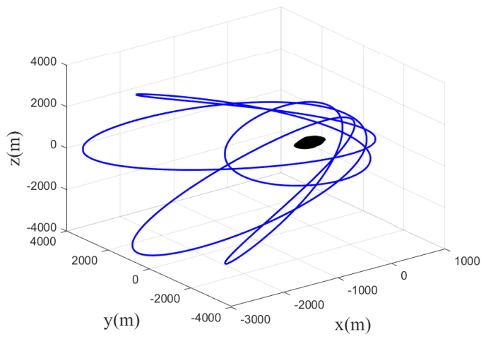
Due to the microgravity environment of asteroids and the perturbation caused by solar radiation pressure, numerous quasi-terminator or quasi-periodic orbits can exist around the asteroid. These orbits exhibit favorable stability properties under solar radiation pressure and are well-suited for global mapping missions around asteroids. In this work, a 4:1 resonant periodic orbit (as shown in Figure 2) is adopted, meaning that the spacecraft completes four revolutions around the asteroid before the orbit closes. The initial position is selected as the lowest point of a quasi-periodic orbit located above the landing site.

During the spacecraft’s proximity operations around the asteroid, the nominal attitude is defined such that the spacecraft’s Z-axis points toward the asteroid, while the X-axis points toward the Sun. This design is based on the attitude-pointing strategy adopted by OSIRIS-REx during the reconnaissance phase. According to the above attitude definition, the quaternion representing the spacecraft body frame relative to the orbital frame can be calculated and further converted into $\varphi$. On this basis, a small perturbation is added to the initial attitude parameters.

The asteroid-shape model data was obtained from http://sbn.psi.edu/pds/shape-models/ (accessed on 1 June 2025). The parameters used in this section are shown in

Table 1. Parameters for TBMPC and TBMPC-FFA.

Parameters	Value
$t_f$	600 s
$\rho$	1260 kg/m3
${\beta }_{SRP}$	1.7744 × 1015
R	1.685 × 1011 m
N	30
$\Delta t$	2 s
$\varphi$	${70}^{\circ }$
${\theta }_{LOS}$	${80}^{\circ }$
$u_{max}$	0.55 m/s2
$T_{max}$	3 Nm
$ϵ$	1$\times {10}^{-3}$
${\mathit{Q}}_{\mathit{p}}$	${\mathit{I}}_6$
${\mathit{Q}}_{\mathit{r}}$	${\mathit{I}}_3$
${\mathit{R}}_{\mathit{p}}$	${10}^3{\mathit{I}}_6$
${\mathit{R}}_{\mathit{r}}$	${10}^4{\mathit{I}}_3$
${\lambda }_p$	0.96
${\lambda }_r$	0.98
${\widehat{\mathit{w}}}_{p,0}$	$\mathit{0}$
${\widehat{\mathit{w}}}_{r,0}$	$\mathit{0}$
${\widehat{\Sigma }}_{{\mathit{w}}_{\mathit{p}},0}$	$\mathrm{diag}\left(4\times {10}^{-2}{\mathbf{I}}_{1\times 3}{\mathrm{m}}^2,2.5\times {10}^{-3}{\mathbf{I}}_{1\times 3}{\left(\mathrm{m}/\mathrm{s}\right)}^2\right)$
${\widehat{\Sigma }}_{{\mathit{w}}_{\mathit{r}},0}$	$\mathrm{diag}\left(1\times {10}^{-6}{\mathbf{I}}_{1\times 3},1\times {10}^{-8}{\mathbf{I}}_{1\times 3}{\left(\mathrm{rad}/\mathrm{s}\right)}^2\right)$

.

Both state constraints and control input constraints are modeled in polyhedral form. The control constraints for both orbital and attitude dynamics are bounded within a polyhedral set defined by $u_{max}$ and $T_{max}$. The initial and terminal states are listed in

Table 2. The initial and terminal states.

Parameters	Value
${\mathit{r}}_{\mathit{0}}$	[959.2404 162.4966 752.7547] m
${\dot{\mathit{r}}}_{\mathit{0}}$	[7.7649$\times {10}^{-4}$ 0.0844 −0.0192] m/s
${\mathit{\varphi }}_{\mathit{0}}$	[0.3142 2.925 0.3142]
${\mathit{\omega }}_{\mathit{0}}$	[1$\times {10}^{-3}$ 0 3$\times {10}^{-3}$] rad/s
${\mathit{r}}_{\mathit{f}}$	[0 0 246.5] m
${\dot{\mathit{r}}}_{\mathit{f}}$	[0 0 0] m/s
${\mathit{\varphi }}_{\mathit{f}}$	[0 3.1416 0]
${\mathit{\omega }}_{\mathit{f}}$	[0 0 0] rad/s

. In this study, the actuators are assumed to be ideal continuously variable actuators, such that the control forces and torques can vary continuously within the specified bounds. This assumption simplifies the control implementation and does not explicitly account for practical actuator characteristics. Therefore, this assumption represents a limitation of the current study.

The sampling time and the update frequency are both 2 s. The bounded disturbance is modeled as a lumped uncertainty term, mainly including asteroid gravity modeling errors caused by the irregular gravitational field, linearization errors of the nonlinear coupled translational–attitudinal dynamics, actuator execution errors, and other unmodeled dynamics. The disturbance covariance matrix ${\widehat{\Sigma }}_{\mathit{w},0}$ used in this study is adopted from Ref. [28]. Due to the lack of actual flight data and validated disturbance statistics for the asteroid proximity operations considered in this work, the covariance parameters listed in the table are intended to represent typical disturbance levels commonly adopted in the literature rather than the exact disturbance characteristics of a specific mission environment. These disturbance parameters are primarily selected to demonstrate the effectiveness and superiority of the proposed algorithm under uncertain conditions. In future work, as data and references from real asteroid exploration missions become available, the initial disturbance estimation can be further refined and calibrated to better reflect the disturbance characteristics encountered in realistic mission environments. The corresponding parameter values are listed in Table 1.

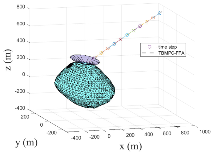
Figure 3 illustrates the close-proximity trajectory with glide-slope constraints, where the circles represent the trajectories over the entire prediction horizon at different update instants. The computational burden of the proposed framework mainly arises from the iterative sequential convex optimization and the online uncertainty identification process. The proposed algorithm converges within an average of two sequential convex optimization iterations at each control step, with an average computation time of approximately 7 s. The current implementation is evaluated in a ground-based simulation environment. According to the simulation results, the average computation time for a single optimization step is approximately 7 s, while the control update period is 2 s. Therefore, the current method does not yet satisfy strict real-time onboard application requirements. Future work will focus on improving computational efficiency through solver optimization and embedded implementation strategies. In addition, adjusting the MPC control update period according to mission requirements and onboard computational capabilities will also be investigated to support practical real-time onboard deployment.

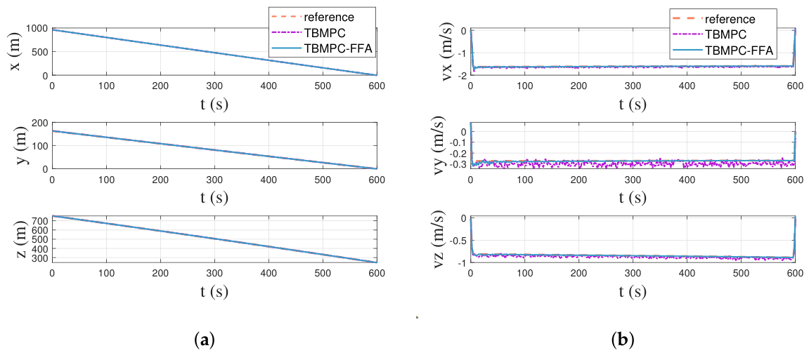
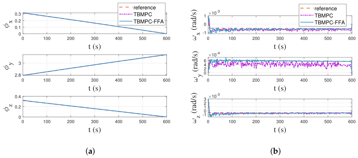
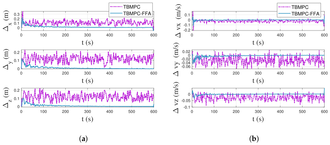
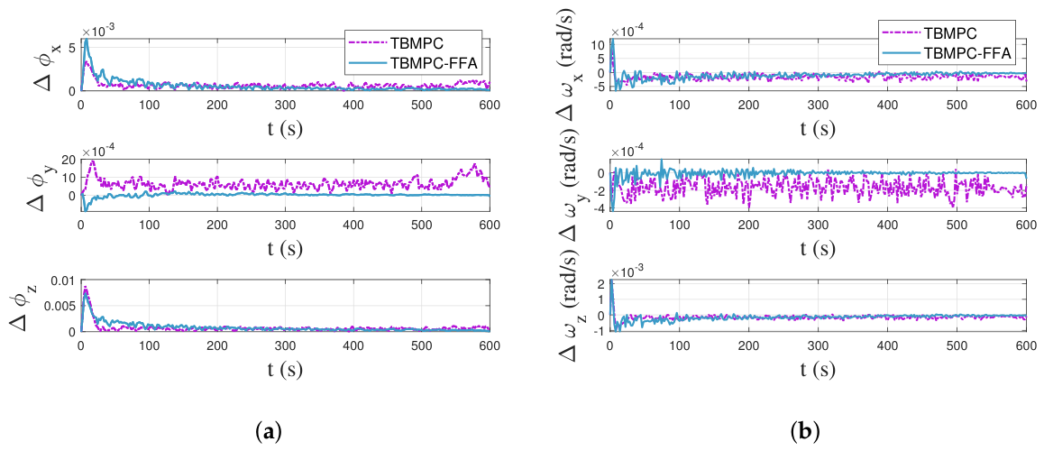
Figure 4 and Figure 5 show the position and attitude trajectories generated by TBMPC-FFA and nominal TBMPC. To more clearly demonstrate the superiority of the proposed algorithm, Figure 6 and Figure 7 further present the tracking errors of TBMPC and TBMPC-FFA with respect to the reference trajectory in Figure 4 and Figure 5. Although the deviations of both methods from the reference trajectory are relatively small, it can still be observed from the figures that TBMPC-FFA achieves better trajectory-tracking performance than TBMPC for the position-related state variables, exhibiting smaller tracking errors. In particular, for the Lie algebra and angular velocity along the y-axis, the nominal TBMPC trajectory exhibits significant deviations from the reference, whereas TBMPC-FFA closely follows it. These observations highlight the improved tracking accuracy of TBMPC-FFA, demonstrating its effectiveness in maintaining tracking accuracy under dynamic conditions.

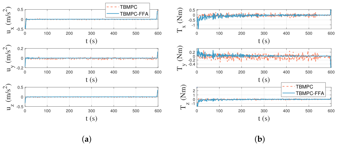
Figure 8 presents the control inputs generated by TBMPC-FFA and nominal TBMPC. For position control, TBMPC-FFA requires smaller input magnitudes compared to the nominal TBMPC, indicating more efficient control. In contrast, for attitude control along the x and z axes, TBMPC-FFA applies significantly larger inputs during the initial phase. This proactive allocation of control effort allows the system to better counteract increased external disturbances, thereby improving disturbance-rejection and overall tracking performance. These observations highlight the superior effectiveness of TBMPC-FFA in achieving precise and robust control.

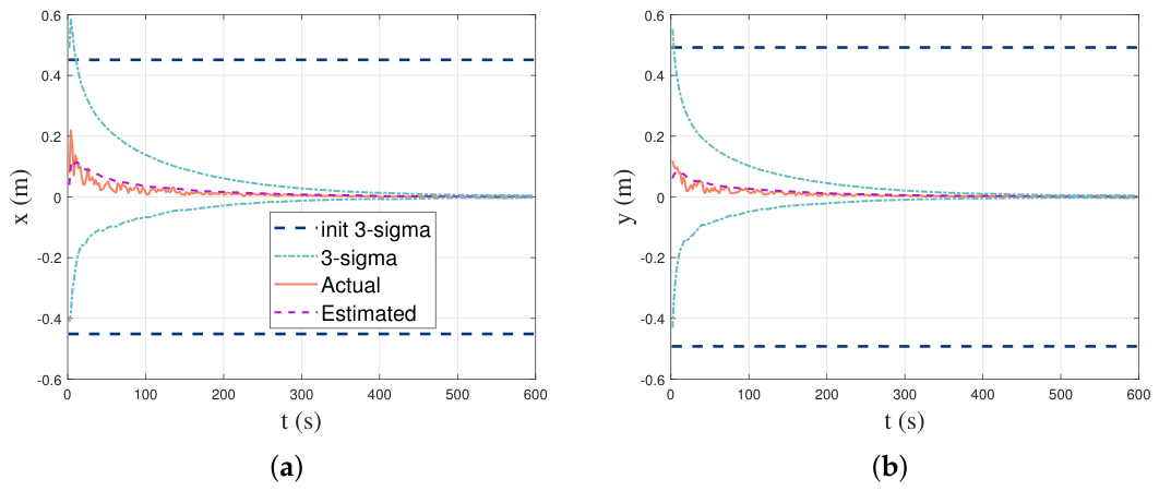
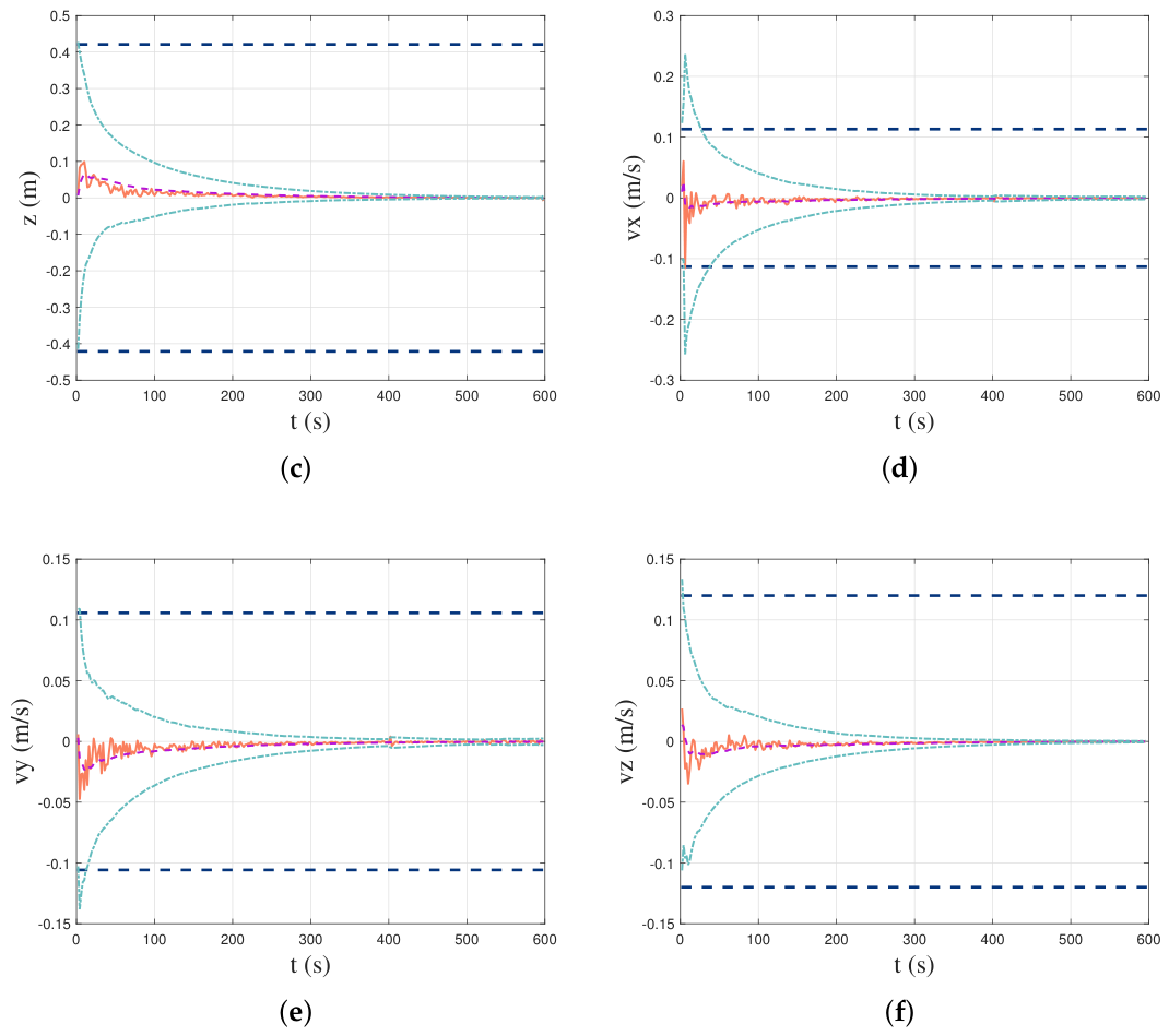
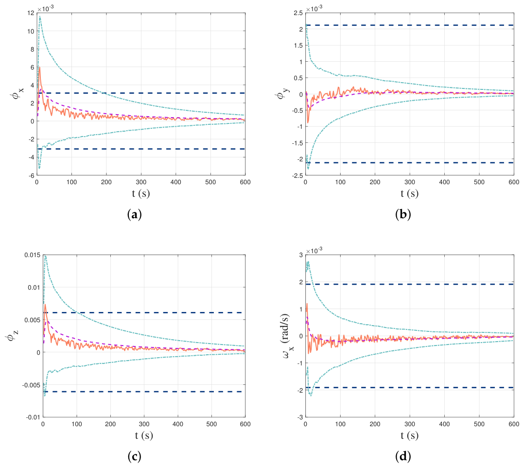
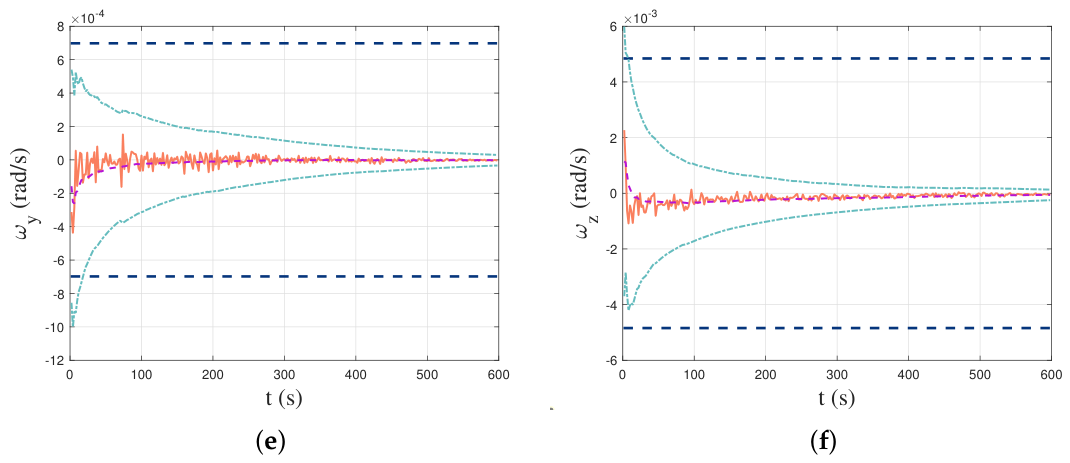
Figure 9 and Figure 10 present the actual and estimated exogenous inputs for position and attitude, along with uncertainty bounds derived from the estimated disturbance covariance. These bounds, proportional to the tube size in each dimension, describe the uncertainty range of the estimates, with dotted lines indicating the nominal TBMPC bounds. Initially, large exogenous inputs cause the tubes to expand. As the estimates converge, the covariance decreases and the bounds shrink, reducing constraint conservativeness. Throughout, the estimated inputs accurately capture the actual disturbance levels. It is worth noting that the disturbance set must enclose the future disturbance; if the disturbance exceeds the boundary, it indicates that the trajectory is not robust. Therefore, the parameters ${\lambda }_p$ and ${\lambda }_r$ need to be tuned to ensure this condition is satisfied. Not all choices of ${\lambda }_p$ and ${\lambda }_r$ can guarantee that the disturbance set contains the future disturbance. We must identify an appropriate set of parameters such that the disturbance set always encloses the future disturbance at all times. Once such a suitable set of parameters is selected, this guarantee becomes deterministic.

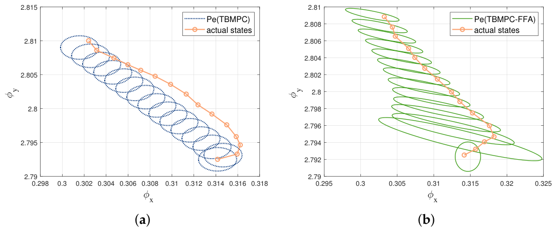
For ${\varphi }_x,{\varphi }_y,{\varphi }_z$ in Figure 11, at certain moments, the exogenous inputs exceed the 3-sigma uncertainty bounds of the nominal TBMPC, indicating that the initial disturbance set ${\widehat{\Sigma }}_{\mathbf{w}}\left(0\right)$ was underestimated relative to the true disturbance range. Consequently, the nominal trajectory does not guarantee robustness, as shown in Figure 10, because the initial tube based on ${\widehat{\Sigma }}_{\mathit{w},\mathit{0}}$ is too small to cover the actual disturbances. In contrast, TBMPC-FFA updates the disturbance set ${\widehat{\Sigma }}_{\mathit{w}}$ online using measured inputs. When actual disturbances exceed the initial estimate, it enlarges the disturbance set and dynamically adjusts the tube size, ensuring robust system behavior.

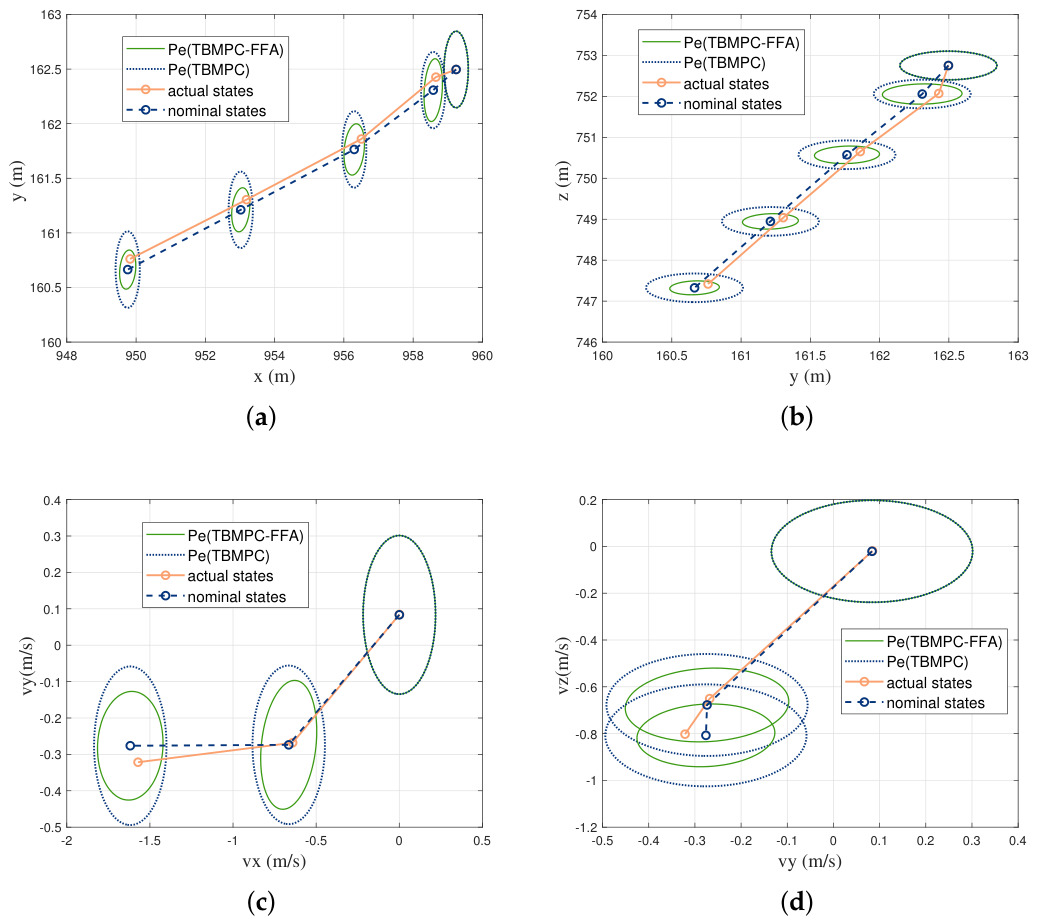
Figure 12 shows the projection of the robust positively invariant (RPI) sets obtained by the nominal TBMPC and TBMPC-FFA onto the x-y plane. To provide a clearer illustration of the relationship between the RPI sets, the actual trajectory, and the reference trajectory, the trajectories are displayed in segments on the x-y plane. The tube generated by the nominal TBMPC remains constant throughout the control process, whereas the TBMPC-FFA tube is adaptively scaled based on the identified exogenous inputs. Simulation results indicate that, at all times, the deviation of the actual trajectory from the reference trajectory remains within the RPI set, satisfying Proposition 1 and thereby ensuring robust tracking performance.

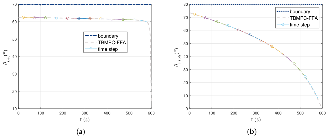
Figure 13 illustrates the glide-slope constraints and line-of-sight constraints. The circles denote the update nodes. For each update node, the plotted trajectory represents the predicted trajectory over the entire prediction horizon N. It can be observed that, at different time instants k, the constraint values within the corresponding prediction horizons are generally consistent with those of the overall trajectory, and they continuously satisfy both the glide-slope constraints and line-of-sight constraints.

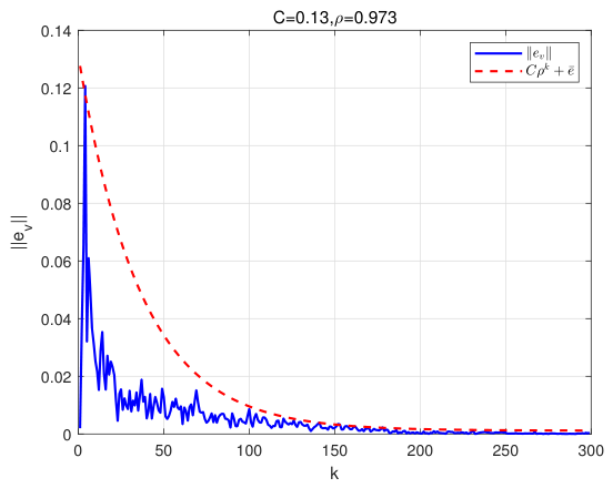
Figure 14 illustrates the convergence of the velocity error, where the constants C and $\rho$ satisfying equation Equation (46) have been determined. In the figure, C in the legend corresponds to $C\parallel e_0\parallel$ the in Equation (46). It can be seen that during the initial stage, the error decays rapidly, exhibiting an overall exponential convergence behavior. In the later stage, the error gradually stabilizes and fluctuates within a small range. This phenomenon is mainly due to the presence of bounded disturbances in the system, which prevent the error from converging to zero and instead constrain it within a bounded set. The exponential upper bound, shown as a red dashed line, consistently lies above the actual error curve, indicating that the system demonstrates good exponential convergence characteristics.

3.3. Sensitivity Analysis

To further analyze the influence of the forgetting factor on the performance of the proposed method, a sensitivity analysis is conducted in this section. By varying the value of the forgetting factor, comparative studies on the tracking performance and control effort of the system are carried out. The corresponding metrics are used to evaluate the effects of different forgetting factors on the robustness and control performance of the system.

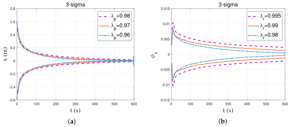
For the scenario considered in this paper, when the forgetting factor $\lambda$ is chosen too small, the computations of the sets $\mathbb{Z}=\mathcal{X}\ominus \mathcal{Z}$ may become infeasible. Therefore, the feasible range of $\lambda$ is limited and can only be selected within a finite interval. In the considered simulation scenario, the optimization problem becomes infeasible when $\lambda <0.95(\lambda ={\lambda }_p,{\lambda }_r)$, indicating that the feasible range of $\lambda (\lambda ={\lambda }_p,{\lambda }_r)$ is approximately [0.95, 1). It should be noted that the feasible interval depends on the specific mission scenario, disturbance magnitude, system constraints, and controller parameter settings. Therefore, the above range is scenario-dependent rather than a universal theoretical bound. Based on this, ${\lambda }_p=0.97,{\lambda }_r=0.99$ and ${\lambda }_p=0.98,{\lambda }_r=0.995$ are selected in this section for sensitivity analysis.

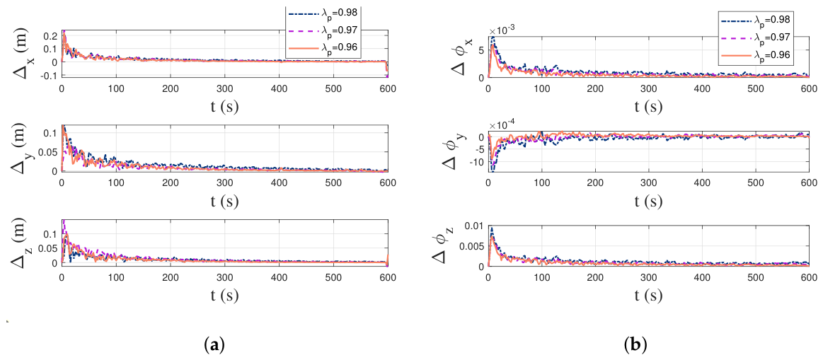
Taking x and ${\varphi }_x$ as examples, Figure 15 and Figure 16 present the error curves and the $3\sigma$ values of the disturbance-invariant sets under different values of $\lambda$, respectively. It can be observed from the error curves that the tracking errors corresponding to different $\lambda$ values are quite similar, whereas the disturbance-invariant set decreases as $\lambda$ decreases.

To quantitatively evaluate the control performance of the proposed method, the following performance indices are introduced to characterize the overall system performance:

$$J_p={\displaystyle \sum _{k=0}^{t_f}}\left({∥{\mathit{x}}_p\left(k\right)-{\overline{\mathit{z}}}_p\left(k\right)∥}_{\mathit{Q}}^2+{∥\mathit{u}\left(k\right)∥}_{\mathit{R}}^2\right)$$

(54)

$$J_r={\displaystyle \sum _{k=0}^{t_f}}\left({∥{\mathit{x}}_r\left(k\right)-{\overline{\mathit{z}}}_r\left(k\right)∥}_{\mathit{Q}}^2+{∥\mathit{T}\left(k\right)∥}_{\mathit{R}}^2\right)$$

(55)

In this equation, both $\mathit{Q}$ and $\mathit{R}$ are chosen as identity matrices. To quantitatively analyze the influence of different $\lambda$ values on system performance, the performance index values in Equations (54) and (55), the total control effort ${\left|\right|\mathit{u}\left|\right|}_2$, terminal error, and root mean square (RMS) error under different $\lambda$ values are further compared. The detailed values of the performance metrics under different $\lambda$ values are listed in

Table 3. Performance comparison under different $\lambda$ values.

		J	Total Control Effort (m/s2/Nm)	Terminal Error (m, m/s, /, rad/s)	RMS (m, m/s, /, rad/s)
TBMPC	Position	16.2627	1.8441	0.1865 0.1192	0.2148 0.0620
	Attitude	16.3634	6.9919	0.0013 3.5802$\times {10}^{-4}$	0.0016 3.7628$\times {10}^{-4}$
${\lambda }_p=0.96$	Position	1.4787	1.5734	0.0686 0.0885	0.0374 0.0130
	Attitude	21.2822	7.4815	1.8661$\times {10}^{-4}$ 7.8690$\times {10}^{-5}$	0.0016 3.2974$\times {10}^{-4}$
${\lambda }_p=0.97$	Position	1.5708	1.5861	0.1393 0.1026	0.0397 0.0143
	Attitude	22.2176	7.6231	4.1732$\times {10}^{-4}$ 2.6344$\times {10}^{-4}$	0.0018 3.8261$\times {10}^{-4}$
${\lambda }_p=0.98$	Position	1.6187	1.5815	0.1389 0.1254	0.0419 0.0154
	Attitude	24.2805	8.0887	5.8147$\times {10}^{-4}$ 2.1704$\times {10}^{-4}$	0.0021 4.507$\times {10}^{-4}$

.

As shown in Table 3, compared with the conventional TBMPC, the proposed TBMPC-FFA achieves significant improvements in position-related performance metrics. The position performance index decreases from 16.2627 to approximately 1.5–1.6, corresponding to a reduction of about 90%. In addition, the terminal position error is reduced by approximately 30–60%. The terminal velocity error shows a noticeable improvement only when $\lambda =0.96$ and $\lambda =0.97$, with a reduction of approximately 14–45%. Meanwhile, the root mean square (RMS) errors of both position and velocity are reduced by about 80%. The total control effort is slightly reduced. Meanwhile, both the terminal error and RMS are significantly decreased. These results indicate that TBMPC-FFA improves position-tracking accuracy and reduces position control effort while maintaining system robustness. In addition, as $\lambda$ increases, the disturbance-invariant tube gradually expands, and the performance index values, total control effort, terminal error, and RMS for both position and attitude all exhibit increasing trends. This indicates that a smaller $\lambda$ can generate a tighter disturbance-invariant tube, thereby reducing the deviation between the actual trajectory and the nominal trajectory and achieving higher tracking accuracy and lower control effort while satisfying robust constraints.

Regarding the attitude control effort, although TBMPC-FFA requires relatively larger attitude torques, this behavior improves the robustness of the closed-loop system by ensuring that the actual trajectory remains within the disturbance-invariant tube under bounded disturbances. In contrast, the conventional TBMPC achieves lower attitude control consumption, but part of the actual trajectory violates the robustness requirement, i.e., it partially exceeds the disturbance-invariant tube (Figure 11). Therefore, the additional attitude control effort in TBMPC-FFA can be interpreted as a trade-off between control consumption and robust constraint satisfaction.

3.4. Monte Carlo Analysis

To further verify the robustness of the proposed method under bounded disturbances, 100 Monte Carlo simulations are added in this paper. In each simulation run, the disturbances are randomly sampled according to Equation (18), and the actual system trajectory is propagated accordingly. By analyzing the trajectory distributions under different disturbance realizations, it is verified whether the actual trajectories always remain within the boundary of the robust invariant set.

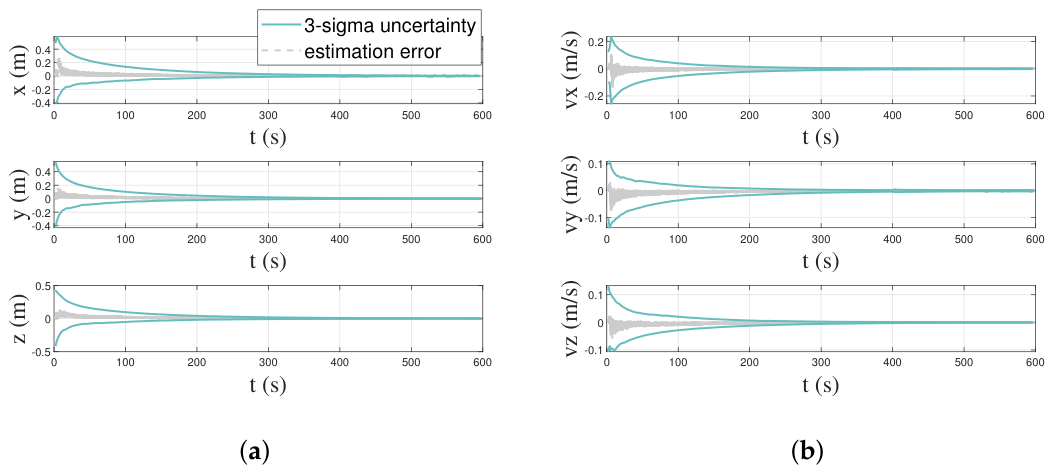
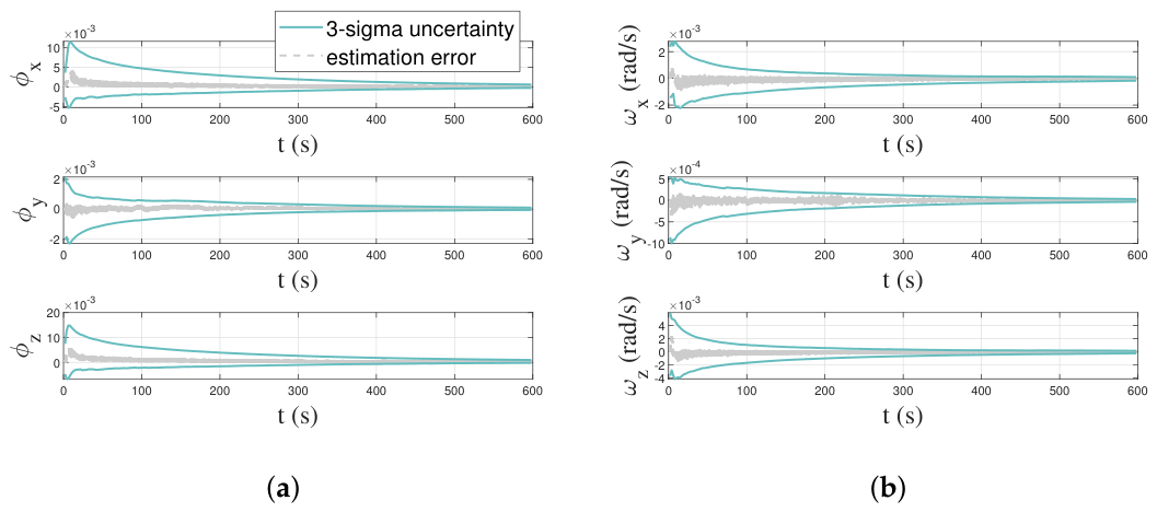
The figure presents the $3\sigma$ boundary of the disturbance set corresponding to ${\lambda }_p=0.96, {\lambda }_r=0.98$ together with 100 Monte Carlo simulation trajectories to verify the robustness of the proposed method. As shown in Figure 17 and Figure 18, the trajectories generated from 100 Monte Carlo simulations all remain within the boundary of the robust invariant set, which demonstrates that the proposed method can effectively guarantee system robustness and constraint satisfaction under the bounded disturbance condition defined in Equation (18). In Figure 17a, the position errors are all positive during the initial stage, causing the error curves to remain above zero. As the system gradually stabilizes, the position errors converge to the vicinity of zero and exhibit small fluctuations during the latter part of the simulation. Due to the scale and resolution of the original figure, these small-amplitude fluctuations are not clearly visible.

Table 4. Monte Carlo simulation statistics.

Performance Indices	Statistic	TBMPC	TBMPC-FFA
Position $J_p$	Mean	12.2953	1.1763
	$3\sigma$	0.9761	0.1054
Attitude $J_r$	Mean	16.4749	20.9028
	$3\sigma$	2.3100	2.88102

presents the Monte Carlo statistical results of the performance indices for the TBMPC and TBMPC-FFA methods. Compared with TBMPC, TBMPC-FFA significantly improves the position performance. The mean value and the 3 $\sigma$ statistic of the position performance index $J_p$ are reduced by approximately 90.4% and 89.2%, respectively, indicating substantial improvements in both tracking accuracy and robustness.

The Monte Carlo simulations are conducted to evaluate the statistical performance and robustness of the proposed method under uncertain conditions. The results demonstrate that the proposed TBMPC-FFA not only achieves a lower mean position performance index but also significantly reduces the corresponding 3 $\sigma$ value, indicating reduced sensitivity to disturbances and improved consistency across different uncertainty realizations. Therefore, the Monte Carlo results provide statistical evidence that the proposed method offers enhanced robustness and position-tracking performance compared with the conventional TBMPC.

According to the results presented in the table, the attitude control effort obtained from the Monte Carlo simulations is consistent with the conclusions drawn from the nominal simulations. Specifically, TBMPC-FFA achieves a significant improvement in position-tracking performance, while the attitude control effort is slightly higher than that of the conventional TBMPC. This observation is consistent with the previous analysis: although the larger attitude control torques increase energy consumption, they effectively ensure that the actual trajectory remains within the disturbance-invariant tube, thereby preserving the robustness of the system. Therefore, the Monte Carlo simulation results further validate the robustness of the proposed method under bounded disturbances and are in good agreement with both the theoretical analysis and the nominal simulation results.

It should be noted that the proposed method assumes that the uncertainties can be represented within bounded disturbances. Therefore, its applicability may be limited in scenarios involving large epistemic uncertainties or severe model mismatch.

To further extend the proposed framework, state-estimation uncertainty can be incorporated through covariance-based constraint tightening or chance-constrained MPC formulations. In these approaches, the estimation error is typically characterized by a covariance matrix and propagated over time to quantify the uncertainty of the system state. The resulting chance constraints can then be transformed into deterministic equivalent constraints, leading to a stochastic MPC formulation. Nevertheless, it represents an important direction for future research toward a fully integrated navigation–control framework.

4. Conclusions

This paper addresses the problem of robust trajectory tracking for asteroid proximity exploration missions under bounded external disturbances and proposes a disturbance-identification-based tube nonlinear model predictive control method. For the six-degree-of-freedom translational–attitudinal coupled nonlinear dynamics model of the spacecraft, the inner layer employs a sequential convex optimization-based nonlinear MPC framework to solve the nominal trajectory optimization problem, while the outer layer dynamically estimates the disturbance set through an online external disturbance identification mechanism and adaptively adjusts the size of the disturbance-invariant tube, thereby effectively reducing the conservatism introduced by conventional TBMPC with fixed disturbance bounds.

By constructing a robust positively invariant (RPI) set, a tube-based robust constraint mechanism is established to ensure that the actual trajectory remains within the vicinity of the nominal trajectory under bounded disturbances, thereby guaranteeing strict satisfaction of both state and control constraints. To address the complex mission requirements during asteroid proximity operations, glide-slope constraints and line-of-sight constraints are further incorporated to improve the safety and feasibility of trajectory planning.

Simulation results demonstrate that the proposed method can effectively guarantee system robustness and constraint satisfaction under bounded external disturbances. Compared with the conventional TBMPC, the proposed TBMPC-FFA exhibits significant advantages in position-related performance metrics. In addition, the sensitivity analysis indicates that a smaller $\lambda$ can generate a tighter disturbance-invariant tube, thereby reducing the deviation between the actual trajectory and the nominal trajectory and significantly improving the position-tracking performance with lower control consumption under guaranteed robust constraint satisfaction. Although the proposed method requires relatively larger attitude control effort, the additional attitude control torque enhances the robustness of the closed-loop system by ensuring that the actual trajectory always remains within the disturbance-invariant tube under bounded disturbances.

Finally, the robustness of the proposed method is further validated through Monte Carlo simulations. The results show that, under randomly sampled bounded disturbances, all actual trajectories remain within the disturbance-invariant tube, thereby verifying the robustness, stability, and engineering applicability of the proposed method for complex asteroid proximity operation missions.

References

1. Lauretta, D.S.; Balram-Knutson, S.S.; Beshore, E.; Boynton, W.V.; Drouet d’Aubigny, C.; DellaGiustina, D.N.; Enos, H.L.; Golish, D.R.; Hergenrother, C.W.; Howell, E.S.; et al. OSIRIS-REx: Sample Return from Asteroid (101955) Bennu. Space Sci. Rev. 2017, 212, 925–984. [Google Scholar] [CrossRef] [Scilit]
2. Yuichi, T.; Makoto, Y.; Masanao, A.; Hiroyuki, M.; Satoru, N. System design of the Hayabusa 2—Asteroid sample return mission to 1999 JU3. Acta Astronaut. 2013, 91, 356–362. [Google Scholar] [CrossRef] [Scilit]
3. Szmuk, M.; Eren, U.; Acikmese, B. Successive Convexification for Mars 6-DoF Powered Descent Landing Guidance. In Proceedings of the AIAA Guidance, Navigation, and Control Conference, Grapevine, TX, USA, 9–13 January 2017. [Google Scholar]
4. Xie, L.; Zhou, X.; Zhang, H.B.; Tang, G.J. Hybrid-order soft trust region-based sequential convex programming for reentry trajectory optimization. J. Guid. Control. Dyn. 2024, 73, 3195–3208. [Google Scholar] [CrossRef] [Scilit]
5. Zhang, Y.; Zhu, B.; Cheng, M.; Li, S. Trajectory optimization for spacecraft autonomous rendezvous and docking with compound state-triggered constraints. Aerosp. Sci. Technol. 2022, 127, 107733. [Google Scholar] [CrossRef] [Scilit]
6. Sagliano, M. Pseudospectral Convex Optimization for Powered Descent and Landing. J. Guid. Control. Dyn. 2018, 41, 320–334. [Google Scholar] [CrossRef] [Scilit]
7. Sagliano, M. Generalized hp pseudospectral-convex programming for powered descent and landing. J. Guid. Control. Dyn. 2019, 42, 1562–1570. [Google Scholar] [CrossRef] [Scilit]
8. Zhang, Y.; Cheng, M.; Nan, B.; Li, S. Stochastic trajectory optimization for 6-DOF spacecraft autonomous rendezvous and docking with nonlinear chance constraints. Acta Astronaut. 2023, 208, 62–73. [Google Scholar] [CrossRef] [Scilit]
9. Acciarini, G.; Baresi, N.; Lloyd, D.J.B.; Izzo, D. Nonlinear Propagation of Non-Gaussian Uncertainties. J. Guid. Control. Dyn. 2024, 48, 903–913. [Google Scholar] [CrossRef] [Scilit]
10. Jones, B.A.; Doostan, A.; Born, G.H. Nonlinear Propagation of Orbit Uncertainty Using Non-Intrusive Polynomial Chaos. J. Guid. Control. Dyn. 2013, 36, 430–444. [Google Scholar] [CrossRef] [Scilit]
11. Boone, S.; McMahon, J.; Boone, S.; McMahon, J. Directional state transition tensors for capturing dominant nonlinear effects in orbital dynamics. J. Guid. Control. Dyn. 2023, 46, 431–442. [Google Scholar] [CrossRef] [Scilit]
12. Valli, M.; Armellin, R.; di Lizia, P.; Lavagna, M.R. Nonlinear filtering methods for spacecraft navigation based on differential algebra. Acta Astronaut. 2014, 94, 363–374. [Google Scholar] [CrossRef] [Scilit]
13. Zhou, X.; Armellin, R.; Qiao, D.; Li, X. Time-Varying Directional State Transition Tensor for Orbit Uncertainty Propagation. J. Guid. Control. Dyn. 2026, 49, 3. [Google Scholar]
14. Eren, U.; Prach, A.; Koçer, B.B.; Raković, S.V.; Kayacan, E.; Açıkmeşe, B. Model Predictive Control in Aerospace Systems: Current State and Opportunities. J. Guid. Control. Dyn. 2017, 40, 1541–1566. [Google Scholar] [CrossRef] [Scilit]
15. Di Cairano, S.; Park, H.; Kolmanovsky, I. Model predictive control approach for guidance of spacecraft rendezvous and proximity maneuvering. Int. J. Robust Nonlinear Control 2012, 22, 1398–1427. [Google Scholar] [CrossRef] [Scilit]
16. Lee, U.; Mesbahi, M. Constrained autonomous precision landing via dual quaternions and model predictive control. J. Guid. Control. Dyn. 2017, 40, 292–308. [Google Scholar] [CrossRef] [Scilit]
17. Morgan, D.; Chung, S.J.; Hadaegh, F.Y. Model predictive control of swarms of spacecraft using sequential convex programmin. J. Guid. Control. Dyn. 2014, 37, 1725–1740. [Google Scholar] [CrossRef] [Scilit]
18. Morato, M.M.; Feli, M.S. Data Science and Model Predictive Control:: A survey of recent advances on data-driven MPC algorithms. J. Process Control 2024, 144, 103327. [Google Scholar] [CrossRef] [Scilit]
19. Bujarbaruah, M.; Rosolia, U.; Stürz, Y.R.; Zhang, X.; Borrelli, F. Robust MPC for LPV systems via a novel optimization-based constraint tightening. Automatica 2022, 143, 110459. [Google Scholar] [CrossRef] [Scilit]
20. Liao-McPherson, D.; Dunham, W.D.; Kolmanovsky, I. Model predictive control strategies for constrained soft landing on an asteroid. In Proceedings of the AIAA/AAS Astrodynamics Specialist Conference, Grapevine, TX, USA, 13–16 September 2016. [Google Scholar]
21. Specht, C.; Bishnoi, A.; Lampariello, R. Autonomous spacecraft rendezvous using tube-based model predictive control: Design and application. J. Guid. Control. Dyn. 2023, 46, 1243–1261. [Google Scholar] [CrossRef] [Scilit]
22. Mayne, D.Q.; Kerrigan, E.C.; van Wyk, E.J.; Falugi, P. Tube-based robust nonlinear model predictive control. Int. J. Robust Nonlinear Control 2011, 21, 1341–1353. [Google Scholar]
23. Raković, S.V. Model predictive control: Classical, robust, and stochastic. IEEE Control Syst. Mag. 2016, 36, 102–105. [Google Scholar]
24. Lishkova, Y.; Cannon, M. Robust receding horizon control for convex dynamics and bounded disturbances. arXiv 2023, arXiv:2302.07744. [Google Scholar]
25. Mammarella, M.; Capello, E.; Park, H.; Guglieri, G.; Romano, M. Tube-based robust model predictive control for spacecraft proximity operations in the presence of persistent disturbance. Aerosp. Sci. Technol. 2018, 77, 585–594. [Google Scholar] [CrossRef] [Scilit]
26. Rakovi, S.V. The implicit rigid tube model predictive control. Automatica 2023, 157, 585–594. [Google Scholar] [CrossRef] [Scilit]
27. Lopez, B.T. Adaptive Robust Model Predictive Control for Nonlinear Systems. Ph.D. Thesis, Massachusetts Institute of Technology, Cambridge, MA, USA, 2019. [Google Scholar]
28. Oestreich, C.E.; Linares, R.; Gondhalekar, R. Tube-Based Model Predictive Control with Uncertainty Identification for Autonomous Spacecraft Maneuvers. J. Guid. Control. Dyn. 2023, 46, 6–20. [Google Scholar] [CrossRef] [Scilit]
29. Jiang, Y.; Zhou, Q.; He, Y.; Zhang, B. Path-tracking control based on adaptive tube-based robust MPC for high-speed intelligent vehicles. Proc. Inst. Mech. Eng. Part J. Mech. Eng. Sci. 2025, 239, 10016–10033. [Google Scholar] [CrossRef] [Scilit]
30. Sieber, J.; Zanelli, A.; Leeman, A.P.; Bennani, S.; Zeilinger, M.N. Asynchronous Computation of Tube-based Model Predictive Control. IFAC-PapersOnLine 2023, 56, 8432–8438. [Google Scholar] [CrossRef] [Scilit]
31. Hazra, S. Autonomous Guidance for Asteroid Descent Using Successive Convex Optimisation. Ph.D. Thesis, Delft University of Technology, Delft, The Netherlands, 2019. [Google Scholar]
32. Takahashi, S.; Scheeres, D.J. Autonomous Exploration of a Small Near-Earth Asteroid. J. Guid. Control. Dyn. 2021, 44, 701–718. [Google Scholar] [CrossRef] [Scilit]
33. Yang, H.; Baoyin, H. Fuel-optimal control for soft landing on an irregular asteroid. IEEE Trans. Aerosp. Electron. Syst. 2015, 51, 1688–1697. [Google Scholar] [CrossRef] [Scilit]
34. Scheeres, D.J. Constant Density Polyhedron. In Orbital Motion in Strongly Perturbed Environments: Applications to Asteroid, Comet and Planetary Satellite Orbiters; Publishing House: Berlin/Heidelberg, Germany, 2012; pp. 51–52. [Google Scholar]
35. Polyak, B.T.; Nazin, A.V.; Topunov, M.V.; Nazin, S.A. Rejection of Bounded Disturbances via Invariant Ellipsoids Technique. In Proceedings of the 45th IEEE Conference on Decision and Control, San Diego, CA, USA, 13–15 December 2006. [Google Scholar]
36. Gavilan, F.; Vazquez, R.; Camacho, E.F. Chance-constrained model predictive control for spacecraft rendezvous with disturbance estimation. Control Eng. Pract. 2012, 20, 111–122. [Google Scholar] [CrossRef] [Scilit]
37. Mayne, D.Q.; Seron, M.M.; Raković, S.V. Robust model predictive control of constrained linear systems with bounded disturbances. Automatica 2005, 41, 219–224. [Google Scholar] [CrossRef] [Scilit]
38. Williams, B.; Antreasian, P.; Carranza, E.; Jackman, C.; Leonard, J.; Nelson, D.; Page, B.; Stanbridge, D.; Wibben, D.; Williams, K.; et al. OSIRIS-REx Flight Dynamics and Navigation Design. Space Sci. Rev. 2018, 214, 69. [Google Scholar] [CrossRef] [Scilit]
Figure 1. (a) Glide- slope; (b) Line-of-sight.
Aerospace 13 00523 g001
Figure 2. A 4:1 resonant periodic orbit.
Aerospace 13 00523 g002
Figure 3. Close-proximity trajectory with glide-slope constraints.
Aerospace 13 00523 g003
Figure 4. TBMPC, TBMPC-FFA and nominal trajectory: (a) position; (b) velocity.
Aerospace 13 00523 g004
Figure 5. TBMPC, TBMPC-FFA and nominal trajectory: (a) Lie algebra; (b) angular velocity.
Aerospace 13 00523 g005
Figure 6. Error between the trajectories generated by TBMPC and TBMPC-FFA and the reference trajectory: (a) position; (b) velocity.
Aerospace 13 00523 g006
Figure 7. Error between the trajectories generated by TBMPC and TBMPC-FFA and the reference trajectory: (a) Lie algebra; (b) angular velocity.
Aerospace 13 00523 g007
Figure 8. The control input of TBMPC and TBMPC-FFA: (a) force; (b) torque.
Aerospace 13 00523 g008
Figure 9. Estimated values of the exogenous input: (ac) position; (df) velocity.
Aerospace 13 00523 g009aAerospace 13 00523 g009b
Figure 10. Estimated values of the exogenous input: (ac) Lie algebra; (df) angular velocity.
Aerospace 13 00523 g010aAerospace 13 00523 g010b
Figure 11. Positively invariant sets of TBMPC and TBMPC-FFA and actual states: (a) TBMPC; (b) TBMPC-FFA.
Aerospace 13 00523 g011
Figure 12. Robust trajectories: (a) x-y plane; (b) y-z plane; (c) vx-vy; (d) vy-vz.
Aerospace 13 00523 g012
Figure 13. Two constraint values and their boundaries: (a) glide-slope constraint; (b) line-of-sight constraint.
Aerospace 13 00523 g013
Figure 14. Exponential convergence of velocity error.
Aerospace 13 00523 g014
Figure 15. Error trajectories corresponding to different values of λ : (a) position; (b) Lie algebra.
Aerospace 13 00523 g015
Figure 16. Robust invariant set boundaries corresponding to different values of λ : (a) position-x. (b) Lie algebra- ϕ x .
Aerospace 13 00523 g016
Figure 17. Robust invariant set boundary and Monte Carlo trajectories: (a) position; (b) velocity.
Aerospace 13 00523 g017
Figure 18. Robust invariant set boundary and Monte Carlo trajectories (a) Lie algebra. (b) angular velocity.
Aerospace 13 00523 g018