Article

Transformer-Augmented MCTS for Aircraft Landing Problem
by
Jie Hu
1,2,
Shuai Zhang
3,
Xiaorong Feng
3,* and
Xinglong Wang
3
1
The 28th Research Institute of China Electronics Technology Group Corporation, Nanjing 210007, China
2
State Key Laboratory of Air Traffic Management System, Nanjing 210007, China
3
School of Air Traffic Management, Civil Aviation University of China, Tianjin 300300, China
*
Author to whom correspondence should be addressed.
Aerospace 2026, 13(5), 438; https://doi.org/10.3390/aerospace13050438
Submission received: 10 February 2026 / Revised: 14 April 2026 / Accepted: 1 May 2026 / Published: 8 May 2026
(This article belongs to the Special Issue AI, Machine Learning and Automation for Air Traffic Control (ATC))

Abstract

The aircraft landing problem (ALP) poses significant challenges for traditional Monte Carlo Tree Search (MCTS) due to its vast search space and reliance on inefficient random simulations. To overcome these limitations, this paper proposes a novel Transformer-Augmented Monte Carlo Tree Search (TMCTS) algorithm. Our approach integrates a reinforcement learning framework that incorporates key operational constraints, including wake turbulence separation and time windows, and employs a cost function aimed at minimizing both delay time and fuel consumption. A core innovation is the replacement of the conventional random simulation phase in MCTS with a Transformer-based value predictor. This leverages the Transformer’s superior ability to model sequences and capture global dependencies among flights, thereby dramatically accelerating search convergence. Specifically, we designed a two-head Transformer network (comprising policy and value heads) to provide informed prior knowledge, which effectively guides the selection and expansion steps of the MCTS tree. The model is trained within an Actor–Critic framework, utilizing behavior cloning for pre-training followed by reinforcement learning for fine-tuning. Experimental evaluations on the standard OR-Library benchmark demonstrate that our TMCTS method significantly reduces scheduling deviation compared to state-of-the-art baselines (including FCFS, DPALO+GA, DPALO+PSO, and CPLEX). Moreover, it achieves a 93.7% reduction in computation time relative to the CPLEX method, highlighting its superior efficiency and practical applicability for real-time scheduling.

1. Introduction

In 2024, China’s civil aviation industry achieved a total transport turnover of 1485.17 billion t-km, 730 million passenger trips, and 8.9816 million t of cargo and mail volume, representing year-on-year increases of 25.0%, 17.9%, and 22.1%, respectively. These figures reflect steady growth in the industry’s transportation operations [1]. During the same year, Chinese passenger airlines operated a cumulative total of 5.0031 million flights, of which 4.3577 million were punctual, resulting in an average flight punctuality rate of 87.1%. Runway resource constraints have been identified as a primary cause of flight delays at hub airports, and so this decline in punctuality underscores a pressing need to enhance runway throughput and scheduling efficiency [2].
To mitigate the risks posed by wake turbulence during approach and landing phases, aircraft must maintain a minimum separation distance from preceding flights. The International Civil Aviation Organization (ICAO) categorizes aircraft into three classes based on maximum takeoff weight (MTOW):
  • Light (L): MTOW less than 7 t;
  • Medium (M): MTOW between 7 and 136 t;
  • Heavy (H): MTOW greater than 136 t.
The wake vortices generated by a leading aircraft can significantly affect the takeoff and landing performance of following aircraft. Therefore, during the approach phase, the required separation between aircraft must satisfy both the wake turbulence separation minima and the standard aircraft safety separation requirements.
In 2010, Balakrishnan [3] reformulated the wake separation distance criteria into equivalent wake time separation intervals, as detailed in Table 1. This conversion facilitates integration into runway scheduling models.
The core optimization problem addressed in this paper is the determination of an optimal aircraft sequencing schedule. This schedule must do the following:
  • Satisfy all prescribed wake time separation constraints;
  • Minimize the total completion time for takeoff and landing operations;
  • Reduce associated landing costs.
According to references [4,5], the aircraft landing problem (ALP) is subject to two primary constraints:
  • Time Window Constraint: Each flight must land within a specified time interval bounded by an Earliest Landing Time (ELT) and a Latest Landing Time (LLT).
  • Wake separation constraint: Successive landings must adhere to the minimum wake turbulence separation intervals.
The Earliest Landing Time (ELT) is defined as the earliest theoretical time at which the flight could arrive and land without any delays. Conversely, the Latest Landing Time (LLT) represents the maximum allowable time an aircraft can remain airborne, typically involving holding patterns, before it must land [6].
Deviations from an ideal schedule incur operational costs. Landing earlier than planned can increase airport congestion and air traffic controller workload, leading to higher associated labor costs. Landing later typically results in increased fuel consumption due to extended flight time. Consequently, for each flight i, there exists an Optimal Landing Time (Ti) that minimizes the total operational cost. The cost function for flight i is typically modeled as a piecewise linear function:
C i t i = g i × T i t i i f t π i < T π i   ( e a r l y   l a n d i n g ) 0 i f t π i = T π i h i × t i T i i f t π i > T π i   ( l a t e   l a n d i n g )
where ti is the actual landing time, Ei and Li are the Earliest and Latest Landing Time, and gi and hi are the unit costs for earliness and tardiness. This creates a V-shaped convex cost profile centered at Ti, as illustrated in Figure 1.
The ALP is a well-known NP-hard combinatorial optimization problem characterized by multiple operational constraints and strict time-sensitivity requirements. Extensive research has been conducted over the past two decades, leading to the development of various models and solution methodologies. Beasley [7,8] established a foundational mixed-integer programming (MIP) model for the ALP and created the widely used OR-Library benchmark dataset. This dataset formally defines the key temporal parameters—Earliest Landing Time (ELT), Optimal Landing Time (OLT), and Latest Landing Time (LLT)—enabling the optimization of objectives for different stakeholders.
To tackle the computational complexity, numerous heuristic algorithms have been proposed. H. Pinol [9] introduced a population-based heuristic, demonstrating its capability on a large-scale instance with 500 aircraft and 5 runways, though its performance degraded with over 50 aircraft. Sheng-Peng Yu [10] developed a cellular automata-based optimization algorithm, which achieved optimal solutions for small-scale cases (test cases 1–7) and near-optimal solutions for large-scale datasets from the OR-Library. Gui D et al. [11] proposed a novel meta-heuristic for the ALP, integrating tabu search to improve solution quality and a rolling time horizon method to enhance computational speed. Daniel A et al. [12] presented a fast greedy heuristic, the Closest Aircraft Sequence with Time Windows (CAS-TW), designed to minimize total delay while respecting operational constraints through a discretization strategy.
Recognizing the multi-faceted nature of the problem, several studies have incorporated multiple objectives. Chen Xiaodao et al. [13] formulated the problem as an integer linear program and transformed it into a multi-objective optimization, proposing an uncertainty-aware scheduling algorithm. Zhang Junfeng et al. [14] constructed a multi-objective ranking and scheduling model for a Parallel Machine Scheduling (PMS) analogy and proposed a multi-objective Imperial Competition Algorithm (ICA), showing significant improvement over First-Come-First-Served (FCFS). Wang Jianzhong et al. [15] proposed a multi-objective time index model, using a genetic algorithm to minimize overall delay and controller workload by weighting different objectives. Chen K et al. [16] established a multi-objective model for the complex interdependent runway ASP (ASP-CIR) and developed an Improved Multi-Objective Restarted Variable Neighborhood Search (IMORVNS) algorithm.
Recent work has increasingly focused on fairness and integrated arrival–departure operations. Liu Jixin et al. [17] addressed four combined operational scenarios, introducing fairness metrics—“equalized delay time for arrivals” and “equalized satisfaction for departures”—and established a two-level planning model to balance fairness and efficiency. Zhou Dingkai et al. [18] applied reinforcement learning to a static terminal area sequencing model, incorporating “flight satisfaction” to enhance fairness in resource allocation between airports and airlines.
Advanced computational methods have been employed to address large solution spaces and real-time requirements. Kang Rui [19] integrated an EoR (Earliest on Route) approach with sequencing strategies and proposed an S-shaped function-based Adaptive Particle Swarm Optimization (SA-PSO) algorithm to minimize flight delay. Zhang C et al. [20] introduced two prescription analysis methods—Estimation-Trial-Optimization (ETO) and Estimation-Trial-Distributionally Robust Optimization (ETDRO)—to improve the efficiency and robustness of sequencing under uncertainty. Dönmez K et al. [21] applied a Multi-Criteria Decision-Making (MCDM) approach, using the MEREC method for criteria weighting and the MARCOS technique to rank solutions, aiming to find a single objective representing an optimal compromise for all stakeholders. Feng Xiaorong et al. [6] developed a time-window-constrained optimization model and proposed a compact subsequence-based algorithm. This method demonstrated high accuracy and speed for small datasets but exhibited lower computational efficiency on large-scale problems.
Although the aforementioned methods have achieved satisfactory performance in addressing the ALP, their high computational complexity often leads to substantial processing time when handling large-scale instances. This limitation poses significant challenges for real-time scheduling and dynamic adjustments in practical operational environments. Consequently, improving algorithmic efficiency and reducing computational overhead remain critical and unresolved issues in this field of research.
In 2006, French computer scientist Coulom [22] first proposed Monte Carlo Tree Search (MCTS), a heuristic search algorithm designed for optimal decision-making in complex scenarios. MCTS efficiently approximates optimal policies through iterative random sampling and tree structure optimization, without requiring complete prior knowledge of the state space. Initially gaining prominence in artificial intelligence, MCTS has achieved groundbreaking success in domains such as the game of Go [23]. A notable milestone was reached in 2016 when AlphaGo, leveraging MCTS, defeated world champion Lee Sedol 4–1, marking the first time an AI system surpassed top human performance in Go.
Beyond game playing, MCTS has been effectively adapted to various optimization and scheduling problems. For instance, Song Wenshuai et al. [24] addressed the dynamic adjustment of reservoir surface sorting strategies under changing environmental conditions by proposing a method based on deep Monte Carlo Tree Search, which integrates deep neural networks to predict prior action probability and evaluate policies. In railway operations, Wang Guanghui et al. [25] introduced a hybrid reinforcement learning–Monte Carlo Tree Search approach for route optimization, employing a breadth-first followed by depth-first selection strategy to balance global and local benefits. For military logistics, Peng Jian et al. [26] designed a heuristic algorithm incorporating MCTS to optimize task sequences for fleet support, using Monte Carlo Trees to record evaluation outcomes and guide subsequent search directions. Similarly, Yu Ze et al. [27] applied an improved MCTS method to unmanned aerial vehicle (UAV) task planning in complex three-dimensional environments, introducing normalized reward ranges to handle parameter uncertainty and balance exploration versus exploitation. Pang et al. [28] proposed a machine learning-enhanced traveling salesman problem framework aimed at reducing total landing time compared to the FCFS approach.
For ALP, existing Arrival Management (AMAN) systems primarily achieve time sequencing through terminal area spatial path expansion and employ speed management when sufficient planning scope is available. In practice, it typically requires air traffic controllers (ATCs) to perform unified, globally optimized sequencing and scheduling of multiple incoming flights when they enter the radar range (radar visibility) of the airport ATC system, assigning each flight a landing time and corresponding time slot. The most widely used strategy for the ALP is the FCFS rule, which schedules aircraft based on their order of entry into the radar range. Current mainstream algorithms predominantly rely on heuristics [7,8,9,10,11,12,29]. There is a demand for aircraft landing scheduling algorithms based on deep reinforcement learning to minimize landing costs. Therefore, this paper proposes a Transformer-Augmented Monte Carlo Tree Search (TMCTS) algorithm to solve the flight sequencing scheduling problem. By considering constraints such as wake separation standards and time windows, combined with estimated arrival times in the terminal area, the algorithm aims to minimize the total cost of the flight sequence. The TMCTS method is employed to calculate the optimal landing sequence and landing time for each flight, The main contributions of this work are threefold:
  • Model Formulation: A reinforcement learning-based optimization model is established for aircraft sequencing, framing the scheduling task as a sequential decision-making process.
  • Algorithm Design: A novel flight scheduling methodology is proposed, which integrates the structural strengths of the Transformer architecture with the strategic search capability of MCTS.
  • Architecture Innovation: A specialized two-head output module is designed, comprising a policy head, and a value head, to effectively capture the unique dependencies and priority constraints inherent in flight scheduling.
The proposed TMCTS algorithm operates as a deterministic search method, demonstrating strong robustness and stability in handling large-scale scheduling instances. We employed the Airland test case from the OR-Library benchmark to train the model and validate the effectiveness and efficiency of our proposed algorithm. Results were compared against FCFS, heuristic algorithms (GA, PSO, CAO), and a commercial mixed-integer programming (MIP) solver (CPLEX).
The remainder of this paper is organized as follows: Section 2 details the workflow of the proposed TMCTS framework, including its algorithmic architecture and model components. Section 3 describes the experimental setup, covering data sources, parameter configurations, and training procedures. Section 4 presents the computational results and provides a comparative analysis with benchmark methods. Finally, Section 5 concludes the paper by summarizing the findings and suggesting directions for future research.

2. Methodology

2.1. Algorithm Framework

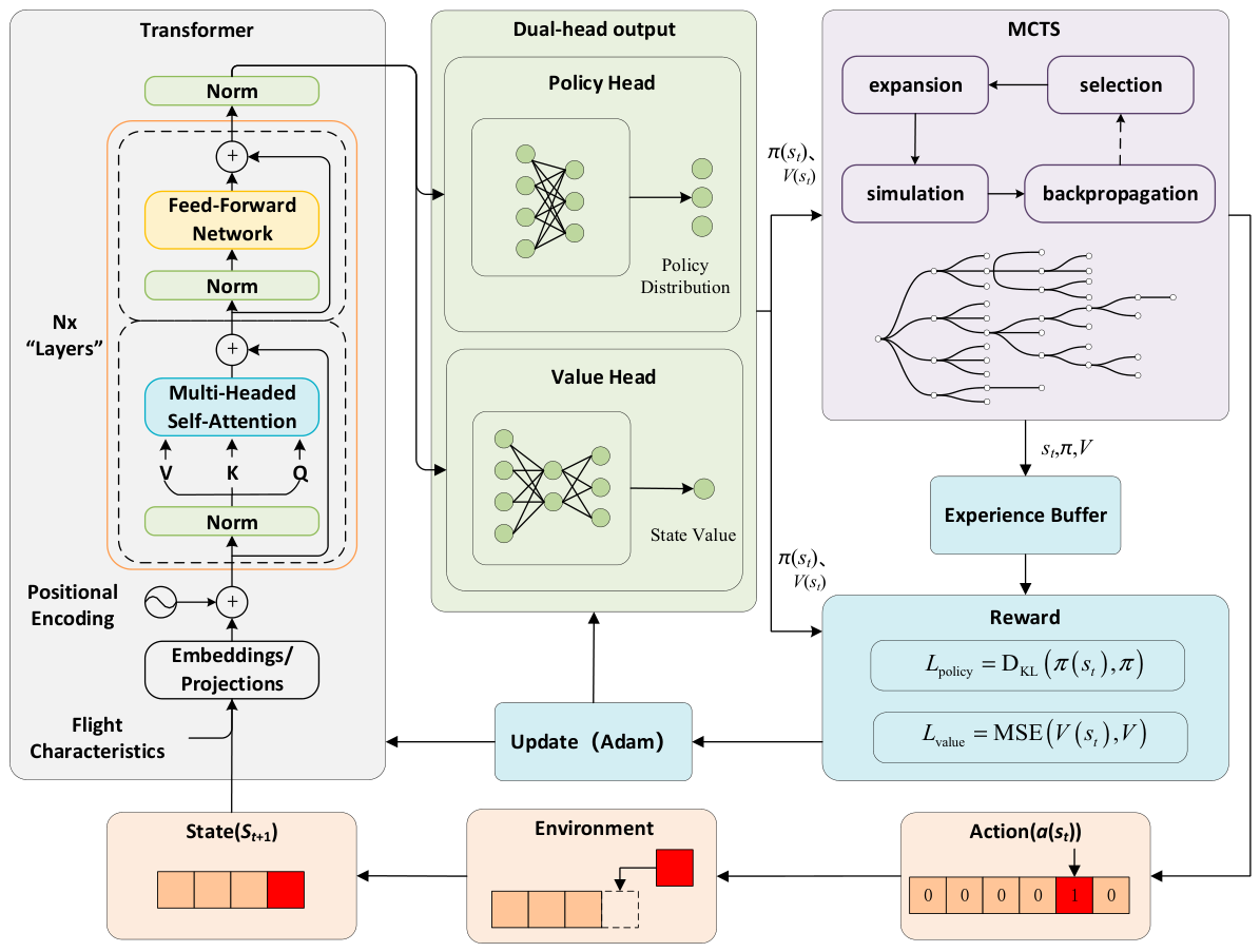
Figure 2 illustrates a deep reinforcement learning-based research framework for flight scheduling, which comprises the following three core components.
  • Transformer-based Scheduling Architecture: Flight data are initially encoded into feature vectors. These vectors are then processed through multiple encoder layers, each consisting of multi-head attention mechanisms and feed forward neural networks, to simultaneously capture the constraints of paired wake separation and the relationship between delay time and cost.
After multi-layer transformations, two output heads generate prior knowledge and state-value estimates, respectively.
2.
MCTS-Guided Strategy Optimization: Leveraging the prior probabilities provided by the Transformer, MCTS iteratively refines flight scheduling strategies through a cyclic process of selection, expansion, simulation, and backpropagation. At each decision node, the improved policy and corresponding value derived from MCTS serve as supervisory signals to train the Transformer network.
3.
Actor–Critic Reinforcement Learning with Transformer Core: An Actor–Critic architecture, integrated with policy gradient methods, employs the Transformer as its central model. Decision-making is guided by MCTS during exploration, while collected trajectory data are used to update the Transformer parameters, thereby facilitating continuous policy optimization for the scheduling agent.
This integrated framework enables synergistic interaction between representation learning, strategic search, and policy improvement, enhancing both the efficiency and robustness of flight scheduling under complex operational constraints.

2.2. Aircraft Landing Issues and Reinforcement Learning Models

2.2.1. Mathematical Model for ALP

This paper focuses on the single-runway, arrival-only aircraft landing problem, where the runway is dedicated to landing operations and departure flights are not considered. The objective of the time-window-constrained multi-flight optimization model is to determine an optimal scheduling sequence π * for N flights and compute the corresponding optimal landing time t π * i for each flight under sequence π * , such that the total cost T C π * N for all N flights is minimized. This objective can be formulated as follows:
T C π * N = argmin t   c π π Π
where N denotes the total number of aircraft to be scheduled, π denotes a candidate landing sequence, Π represents the set of all feasible sequences of N flights, and t c π (total cost) is the minimum total landing cost under sequence π , which can be expressed as
t c π = min i = 1 N f t π i
Here, f t π i represents the cost incurred when the i-th flight in sequence π lands at time t π i , expressed as
f t π i = g π i m a x 0 , T π i t π i + h π i m a x 0 , t π i T π i
where T π i denotes the optimal landing time for flight i under sequence π , and g π i and h π i are the unit cost coefficients for earliness and tardiness, respectively, relative to T π i .
The model is subject to the following operational constraints:
  • Wake separation interval constraint:
t π j t π i S π i , j , i , j 1 , , N , i j
where S π ( i , j ) denote the minimum wake turbulence separation interval between flights i and j under sequence π .
2.
Earliest Landing Time constraint:
t π i E π i , i N
where E π i is the earliest permissible landing time for flight i.
3.
Latest Landing Time constraint:
t π i L π i , i N
where L π i is the latest permissible landing time for flight i.
These constraints ensure that the scheduling sequence respects safety, operational, and time window requirements while minimizing the total landing cost.

2.2.2. Markov Decision Process (MDP) Modeling

The ALP is formulated as a Markov Decision Process (MDP), defined by the quadruple (S, A, R, P):
  • State space
The state space integrates all essential aircraft information and scheduling progress. Each aircraft is represented by a 7-dimensional state vector, defined as
s i t = E π i t , T π i t , L π i t , g π i t , h π i t , m π i t , d π i t
where E π i , T π i , and L π i denote the time window information; g π i and h π i are penalty coefficients; m π i is a binary indicator of whether flight i has been scheduled; and d π i represents the required wake separation between unscheduled flight i and the last scheduled flight.
2.
Action Space
The action space comprises the set of aircraft that can be selected for landing in the current state. A valid action must satisfy two conditions: the aircraft has not yet been assigned a landing, and it complies with safety separation constraints relative to the preceding aircraft. The action space is formally expressed as
A t = a i t | a i t { 0 , 1 } , n a i t = 1
Here ai(t) denotes the action for the i-th flight. ai(t) = 0 indicates that the i-th flight is not selected, while ai(t) = 1 indicates selection.
3.
Reward function
The reward function R(t) is designed to guide the agent toward minimizing cost and completing the scheduling task. It consists of three components:
  • Cost penalty: A negative reward proportional to the cumulative cost incurred at the current scheduling step, with dynamically adjusted weighting throughout the process.
  • Completion reward: A positive reward granted upon successful scheduling of all flights. The global reward is computed using the method described in the previous section for fixed-order ALP, yielding the total cost under the constructed sequence.
  • Deviation Bonus: An additional reward provided when the final scheduling cost outperforms the historical best recorded value.
4.
State transition.
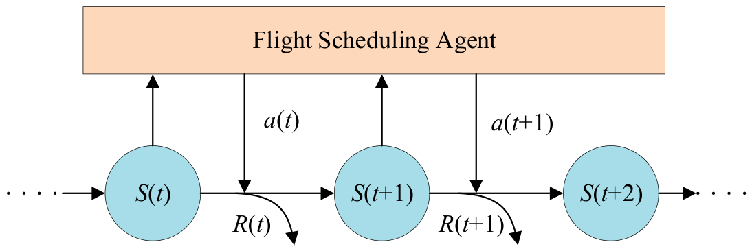
For the current flight scheduling state S(t), after executing action ai(t), the i-th aircraft is marked as “scheduled”; the DPALO module is invoked to calculate the landing time for that aircraft; the flight sequence and the set of unscheduled flights are updated; the wake separation constraints between each unscheduled aircraft and the last scheduled aircraft are calculated; and a new state S(t + 1) is formed. In this paper, action selection follows a stochastic policy with probabilities summing to 1. At each decision step, the agent samples an action a(t) from the action distribution, with the action probability provided by the Transformer’s policy head. The state transition is deterministic: given the current state and the selected next arriving flight, the next state (the set of scheduled flights and the set of remaining unscheduled flights) is uniquely determined, i.e., P(S(t + 1)|S(t),a(t)) = 1. The time period from t to t + 1 represents a discrete decision step in the MCTS process.
The overall reinforcement learning-based decision-making process for flight scheduling is illustrated in Figure 3.

2.3. Solving for Aircraft Landing Times Under Fixed Sequence

ALP can be decomposed into two subproblems: the first is to determine optimal landing time given a sequence, and the second is to find the optimal landing sequence. In the proposed algorithm, MCTS selects an aircraft and appends it to the current landing sequence, and then computes the cost of the resulting partial sequence. At the end of a complete round, the final cost is normalized to the value target range [−1, 1]. This target is then used to train the value head of the Transformer network using mean squared error loss.
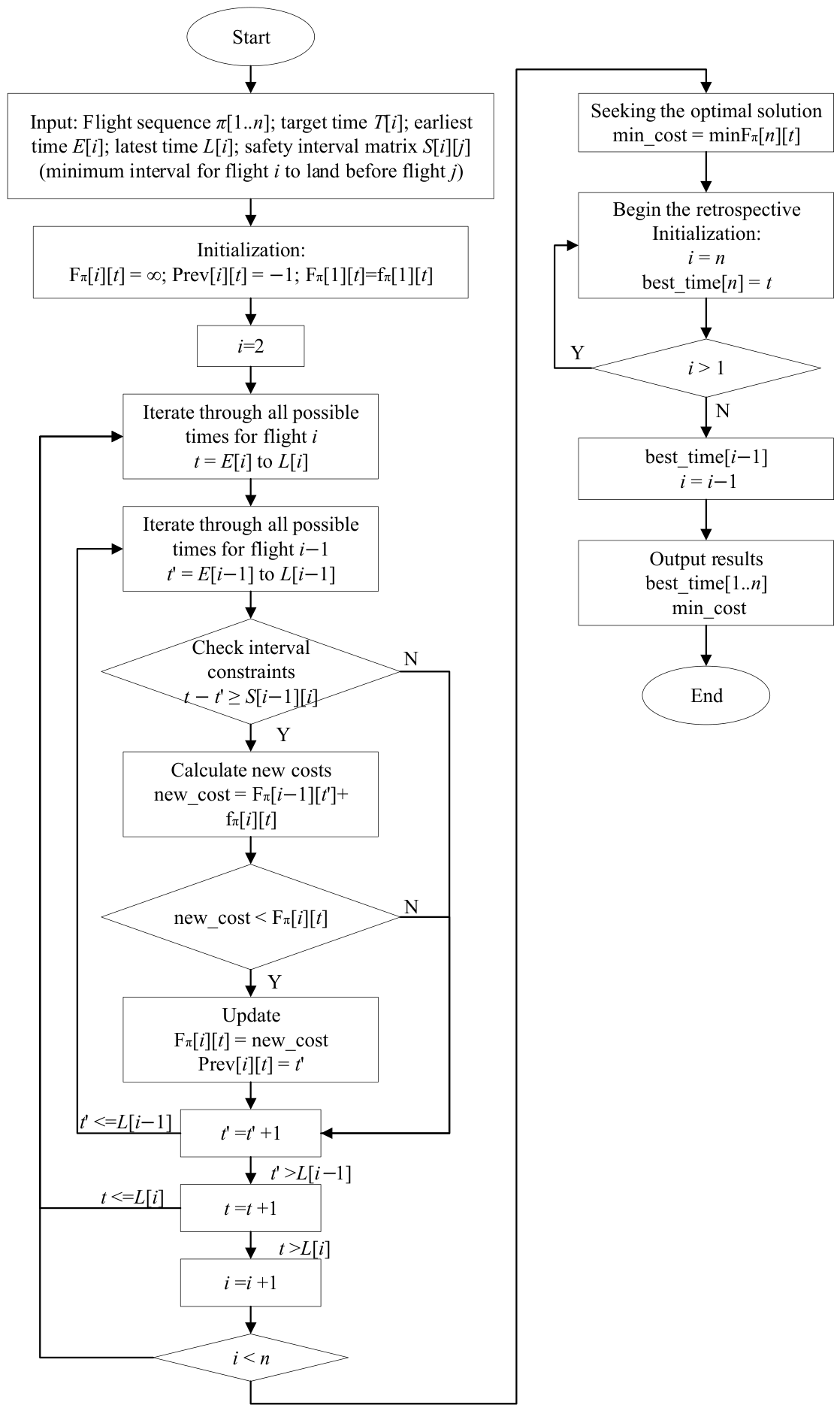
To address the problem of determining aircraft landing times under a fixed sequence, we used the Dynamic Programming Approach to Limit Optimization (DPALO) [29]. First, the landing scheduling problem with a fixed flight sequence is formulated as an integer programming problem for determining the landing time of each flight. This problem is then solved using the Dynamic Programming Algorithm (DPA), which can determine the cost of this sequence with certainty. The DP model consists of N stages (each stage corresponds to a single aircraft). In each stage i, the number of states equals the number of feasible discrete landing times within the time window and interval constraints, with an upper bound determined by the reduced time window length; assuming 1-s discretization, the number of states per stage is ∆T. The total time complexity for solving this fixed-order subproblem is O(N × ∆T).
Let F t π i denote the minimum cumulative total cost generated by the first i flights when the i-th flight in sequence π lands at time t π i . Given that the cost of the first flight in the sequence is F t π 1   =   f t π 1 , the cost of the i-th flight is F t π i = f t π i + min F t π i 1 . Then, establish a time-based recursive function for F t π i as follows:
F t π i = f t π i i = 1 f t π i + min E π i 1 t π i 1 min t π i S π ( i 1 , i ) , L π i 1 F t π i 1 1 < i n
Equation (2) can be further simplified to Equation (11).
t c π = min F t π i π Π
Based on Equations (5) and (6), the range of values for dependent variable t π i of function f t π i is determined to be E π i , L π i . Considering Equation (4) and the optimal value of objective function t c π , the range of values for dependent variable t π i can be further narrowed. This section will further analyze the range of values for dependent variable t π i . Figure 4 shows the flowchart of the dynamic programming algorithm for solving the ALP. In Figure 4, f π [ i ] [ t ] equals f t π i , where f π [ i ] [ t ] represents the cost of landing a flight at that time. For example, f E π i denotes the cost of landing the i-th flight in sequence π at its earliest possible landing time. F π [ i ] [ t ] equals F t π i , where F π [ i ] [ t ] represents the landing time of a flight at that moment and the minimum cumulative total cost generated by all preceding flights. For example, F E π i denotes the minimum cumulative total cost generated by the preceding i − 1 flights when flight i lands at its earliest possible landing time. By calculation, the optimal landing time and total cost for flights under a fixed sequence can be determined.
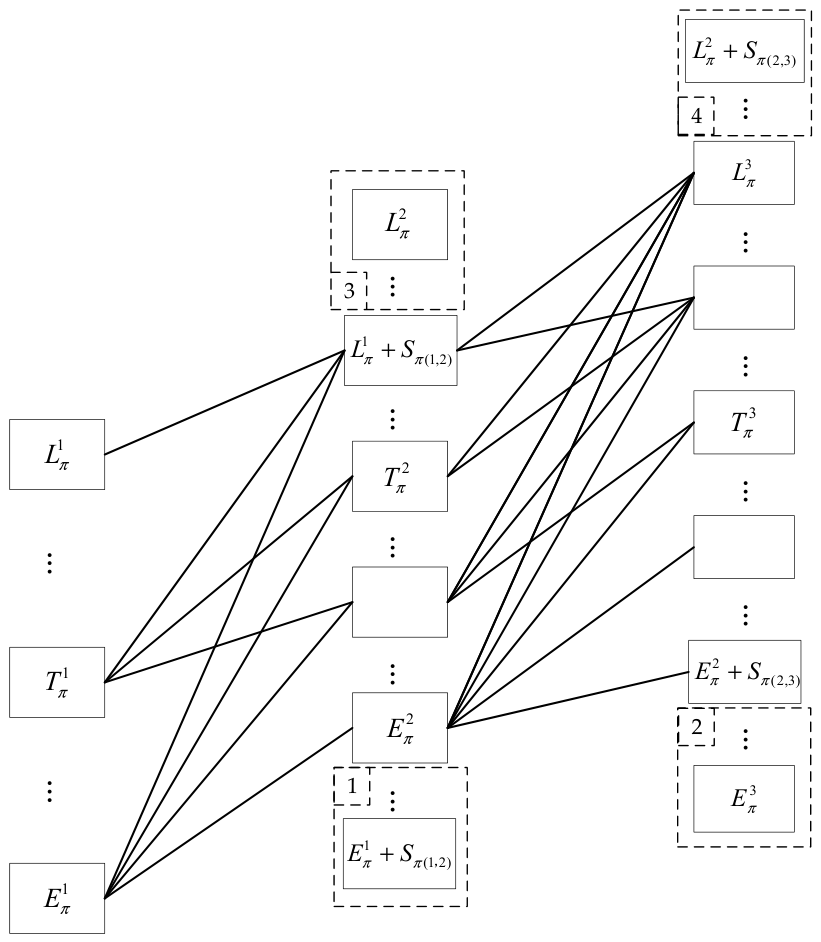
Figure 5 illustrates the search range for flight landing costs under the discretized π sequence, using three flights as an example. Flight landing times must simultaneously satisfy constraints (4), (5), and (6). When E π 2 > E π 1 + S π ( 1 , 2 ) occurs, the second flight cannot land at time E π 2 ,   E π 1 + S π ( 1 , 2 ) , as shown in dashed box 1. When E π 3 < E π 2 + S π ( 2 , 3 ) occurs, the third flight cannot land at time E π 3 ,   E π 2 + S π ( 2 , 3 ) , as shown in dashed box 2. When L π 2 > L π 1 + S π ( 1 , 2 ) occurs, since deviation costs increase linearly with time, f L π 2 > f L π 1 + S π ( 1 , 2 ) holds. Therefore, when calculating the total landing cost for the first two flights, L π 1 + S π ( 1 , 2 ) ,   L π 2 within the second flight’s time window can be omitted from the calculation, as shown in dashed box 3. When L π 1 + S π ( 1 , 2 ) ,   L π 2 occurs, the third flight cannot land at time L π 3 ,   L π 2 + S π ( 2 , 3 ) , as indicated by dashed box 4.
Proposition 1.
Let  π  denote a fixed landing sequence for flights. Under constraints (3), (4), and (5), sequence  t = { t π i * | i = 1 , 2 , 3 , , n ) }  represents the landing times  t c π = i = 1 n f ( t π i * ) = min F t π n = F t π n *  for each flight that minimize  t c π . Then,  t π 1 * T π 1 . Prove by contradiction as follows: First assume that under sequence  π , there exists sequence  t = { t π 1 | i = 1 , 2 , 3 , , n }  such that the minimum value  t c π  is obtained,  t c π = i = 1 n f ( t π i ) , and  t π 1 > T π 1 . Then, the landing time of the first flight is advanced from  t π 1  to  T π 1 . Since this adjustment does not affect the safety intervals or landing times of subsequent flights, their arrival times remain unchanged. Thus, the  π  sequence lands in the order determined by  t = { T π 1 , t π 1 , , t π n } . At this point,  t c π = f ( T π 1 ) + i = 2 n f ( t π i ) = 0 + i = 2 n f ( t π i ) < h π 1 × t π 1 T π 1 + i = 2 n f ( t π i ) , and sequence  t  can achieve a lower cost. Assuming this contradicts Proposition 1,  t π 1 T π 1  is proven. The time window for the first flight can be optimized to  E π 1 ,   T π 1 .
Inference 1.
Similarly, by contradiction, the optimal landing time for the last flight n cannot be earlier than its Earliest Landing Time. Therefore, the time window for the nth flight can also be constrained to optimize to  T π n ,   L π n  
Inference 2.
Based on Proposition 1, Corollary 1, Constraint (3), and Constraint (4), Equations (12) and (13) can be derived.
e π i = T π i i = n max E π i , min T π i , e π i + 1 S π ( i + 1 , i ) i < n
l π i = T π i i = 1 min L π i , max T π i , l π i 1 + S π ( i 1 , i ) i > 1
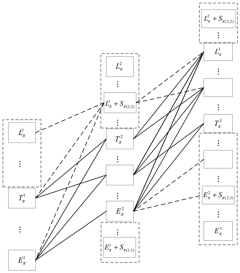
Inference 2 provides the landing time window e π i , l π i after boundary optimization. Figure 6 shows the search range after boundary optimization, using three flights as an example. For Flight 1, the search range is narrowed to E π 1 , T π 1 ; for Flight 3, it is narrowed to T π 3 , L π 3 . For Flight 2, if T π 2 > e π 3 S π ( 2 , 3 ) , E π 2 > e π 3 S π ( 2 , 3 ) and T π 2 > l π 1 + S π ( 1 , 2 ) occurs, its search range is narrowed to E π 2 , T π 2 . The dashed box indicates the search range eliminated compared to DPA optimization, while the dashed line denotes omitted search steps. The search strategy for the remaining portions remains unchanged. The search range required to find the minimum landing cost for the first i + 1 flights also correspondingly decreases, t c π i + 1 = min F e π i + 1 , , F l π i + 1 . Compared to DPA, this approach significantly reduces computational steps and simplifies algorithmic complexity.
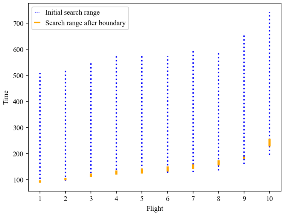
Figure 7 shows the initial time windows [ E π i , L π i ] and the boundary-optimized time windows [ e π i , l π i ] for 10 flights in the Airland1 dataset from OR-Library [7]. The dashed lines indicate the search range for DPA, while the solid lines represent the search range for DPALO. Boundary optimization significantly reduces the computational scope of the algorithms. It reduces ∆T and lowers the algorithm’s complexity.

2.4. Solving for the Optimal Landing Sequence

2.4.1. Monte Carlo Tree Search

To solve for the optimal landing sequence, the TMCTS approach is employed. The landing cost computed using the method in Section 2.3 serves as the primary optimization metric for evaluating candidate landing sequences during the MCTS.
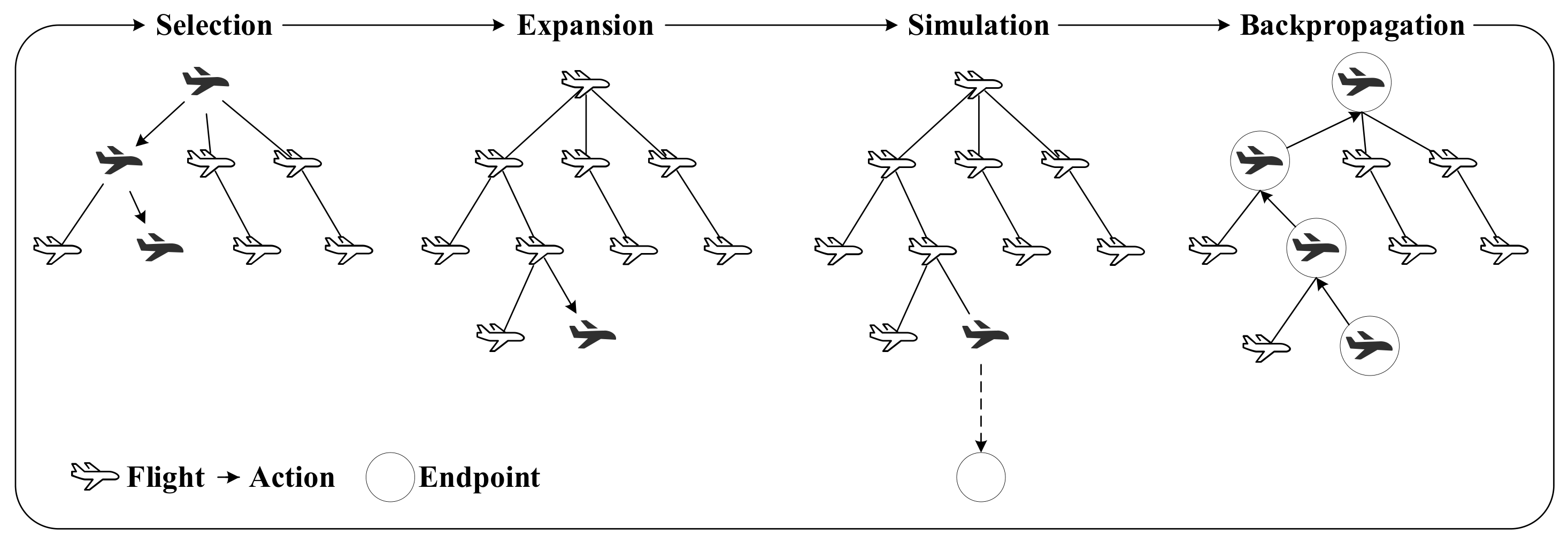
MCTS is a heuristic search algorithm based on random simulation and tree structures, particularly suitable for scenarios with large state spaces where exhaustive search methods are computationally infeasible. Figure 8 illustrates the workflow of the MCTS process. The specific steps are as follows:
(1) Selection. Starting from the root node, where a “node” represents a scheduling state at a given decision step. The algorithm traverses downward through the tree structure to identify a node worthy of further exploration. The core action selection principle is based on the Upper Confidence Bound (UCB), which balances exploration and exploitation. The UCB formula is defined as follows:
UCB =   Q n N n + C × ln N p n N n
Among these, Q(n) represents the cumulative reward of node n; N(n) denotes the number of visits to node n; Q n N n is the utilization term; C is the exploration coefficient; Np(n) indicates the number of visits to the parent node; ln N p n N n is the exploration term.
Traditional MCTS relies on fully random simulations to evaluate node values, resulting in numerous futile searches that reduce computational efficiency. This paper employs a Transformer to generate action policies, state value estimates, and specialized decisions, providing MCTS with prior probabilities. This optimizes search logic during expansion and simulation phases, reducing ineffective exploration. The optimized UCB formula is
UCB = Q n N n + C × p a × ln N p n N n
Among these, p(a) is the prior probability of selecting action a at node n.
(2) Expansion. When node n is not in a terminal state and unexplored actions exist, perform tree extension on node n. Randomly select an action a from the unexplored action set of node n, generate the corresponding child node n′, and initialize the utility and exploration values of the new node. After simulation, proceed with scoring. The scoring calculation process for each node is as follows:
Q = V a l n n × e c c g c g
Among these, Valnn is the normalized cost advantage of the value-head output (with a range of [−1, 1]); a higher value indicates that the expected final cost of the current sub-sequence is more favorable than the Target Time Sequence (TTS) baseline. c represents the cost of selecting this node, and cg represents the cost of TTS at this step. TTS is a sorting method that arranges flights to land in the target time order and serves as the baseline for evaluation.
(3) Simulation. The potential reward of a newly expanded node n′ is rapidly evaluated through simulation. Starting from node n′, actions are continuously executed according to a predefined policy until a terminal state is reached, ultimately yielding the reward value R for that trajectory. By repeatedly performing simulations, MCTS progressively explores different ordering strategies.
(4) Backpropagation. During the backpropagation phase, the reward R obtained from the simulation is propagated backward through all ancestral nodes along the path (from n′ back to the root node). This process updates the node ratings and visit counts of each node, providing evaluation criteria for subsequent selection phases.
By iteratively executing these four steps, a search tree is progressively constructed. Through a finite number of iterations, the tree structure gradually converges toward high-value paths, ultimately yielding an optimal sequencing result.

2.4.2. Transformer Architecture

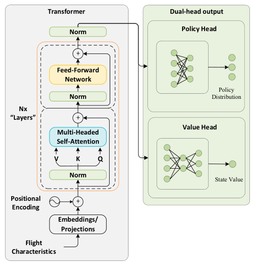
The ALP involves multiple constraints, strong interdependencies, and sequential dependencies. This paper proposes a Transformer-based flight sequencing algorithm. The Transformer architecture is primarily employed to address aircraft scheduling decisions by capturing the features and interdependencies of each aircraft within the sequence. It outputs action policies and state values, providing prior probabilities for MCTS.
The Transformer architecture, as illustrated in Figure 9, primarily consists of two components:
(1) Transformer Encoder
The model architecture consists of stacked encoder layers, each comprising a multi-head attention module, a feed forward neural network, residual connections, and layer normalization. Through multi-layer stacking, feature encoding progressively becomes more abstract and global in scope.
The Embeddings Projections Layer maps the multidimensional features of each flight into a fixed-dimensional space via linear transformation, generating flight feature vectors. This enables the model to process features as numerical representations. Sine–cosine positional encoding is applied to incorporate the positional information of flights within the sequence, endowing the model with awareness of temporal order. Positional encodings are combined with state embeddings before being fed into the model, as defined by the following equations:
P E p o s , 2 i = sin ( p o s 10000 2 i / d model )
P E p o s , 2 i + 1 = cos ( p o s 10000 2 i / d m o d e l )
where pos denotes the position of a flight within the sequence, and i represents the feature dimension index.
The Multi-Headed Self-Attention layer enables each flight feature to attend to all other flight features, capturing global dependencies. It allows the model to identify relationships between aircraft while simultaneously handling interactions between individual and multiple flights. Flight features, after positional encoding and embedding, are used as Query, Key, and Value inputs. Attention weights are computed between each flight and every other flight in the sequence.
The feed forward network layer applies a nonlinear transformation to the output vectors from the self-attention mechanism, enhancing the model’s expressive capacity to learn more complex feature patterns. Residual connections and layer normalization are incorporated to mitigate gradient vanishing during training, ensuring stable feature extraction for flight states.
(2) Multi-Task Output Layer
Based on the learned decision features, the model outputs two types of result. The policy head outputs a probability distribution over aircraft to be selected as the next action, which guides the MCTS in choosing subsequent moves. The value head estimates the value of the current state. This value is used to compute node scores within MCTS.

3. Model Training

3.1. Training Framework

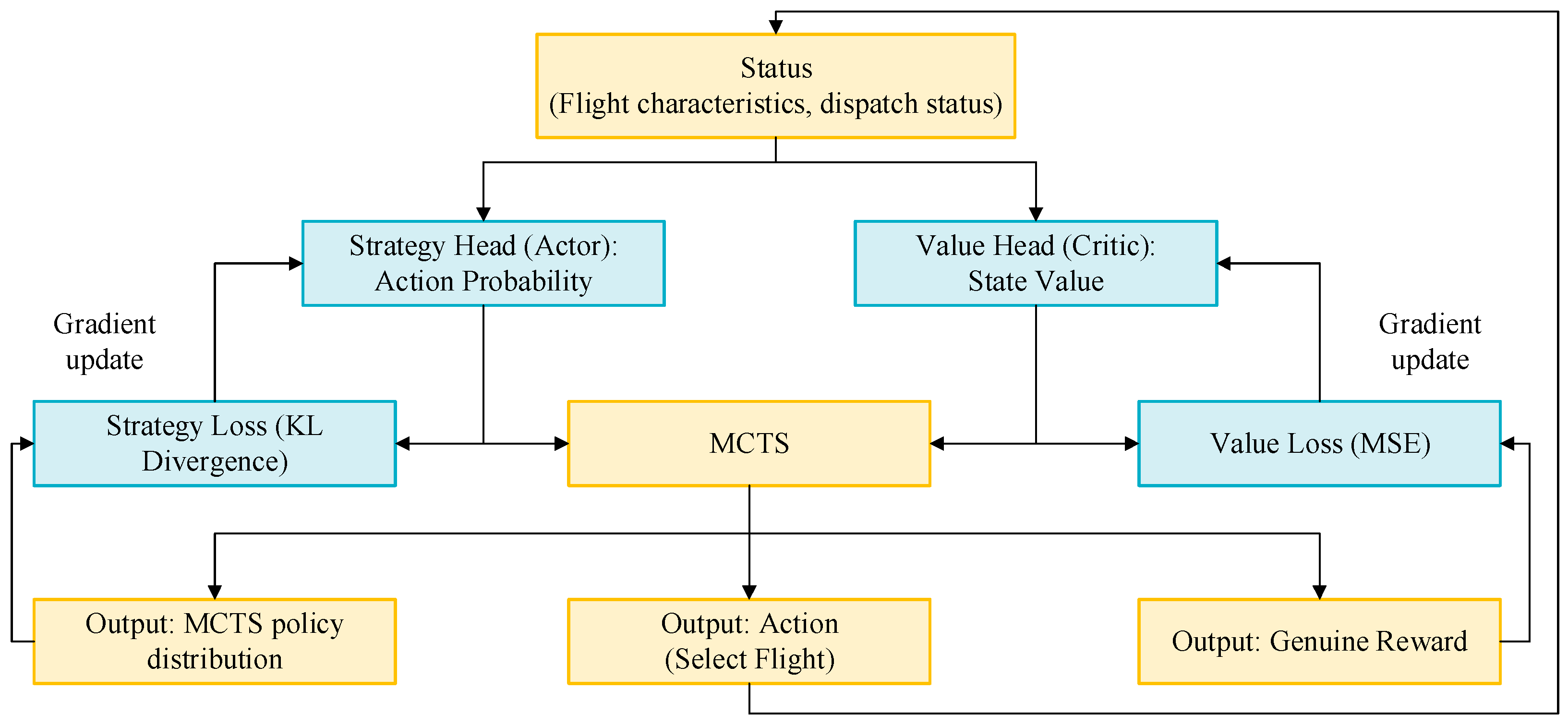
During training, an Actor–Critic framework guided by MCTS is employed. As illustrated in Figure 10, the Transformer simultaneously outputs a policy distribution and a state value estimate. By interacting with the environment to collect data optimized through MCTS, the network is updated via the joint optimization of policy loss and value loss, enabling the agent to improve its policy within the target environment.
First, flight information and state representations are encoded into feature vectors by the Transformer encoder, which outputs both a policy distribution and a value estimate for the current state. The policy output provides prior action probabilities for MCTS, while the value estimate guides MCTS in action selection. MCTS constructs a search tree and ultimately outputs an MCTS policy distribution, a ground-truth value target, and a selected action.
A multi-objective loss function is defined to jointly optimize the policy network and the value network. The policy loss employs Kullback–Leibler (KL) divergence, encouraging the policy network’s prior probabilities to converge toward the optimal action distribution discovered by MCTS through deep search. Value loss is trained using Mean Squared Error (MSE) to bring the value head’s predictions closer to the calculated target values. A target value is calculated for each complete round based on the final scheduling result. If the round generates a feasible landing sequence, the final total cost of that sequence is compared with the cost of the TTS baseline. The difference between the two is scaled to the range [−1, 1] via a tanh transformation: when the final cost is significantly lower than the TTS baseline, the target value approaches +1; when it is on par with the baseline, it approaches 0; it approaches −1 when it is significantly higher than the baseline. If no feasible schedule can be generated, the target value is directly set to −1. The value head is trained to predict this target from any intermediate state, thereby learning to estimate the normalized cost advantage of the current partial sequence.
Network parameters are optimized via gradient descent, with Transformer parameters updated through backpropagation. Through multiple training iterations, the network progressively approximates the decision-making capability and value estimation accuracy of MCTS.

3.2. Experimental Data

The experimental data were obtained from the ALP dataset in J.E. Beasley’s OR-Library, accessible via http://people.brunel.ac.uk/~mastjjb/jeb/orlib/airlandinfo.html (accessed on 20 January 2024). The dataset consists of 13 flight sequences, each containing a varying number of flights. Sequences 1 through 8 constitute the small-scale subset, with 10, 15, 20, 20, 20, 30, 44, and 50 flights, respectively. The remaining five sequences form the large-scale subset, comprising 100, 150, 200, 250, and 500 flights, respectively.
Each flight in the dataset is characterized by seven attributes. The final attribute specifies the required wake separation time interval between the current flight and its predecessor. This information is structured as a matrix where n denotes the number of flights, and nij represents the wake separation interval required for flight j to follow flight i. The value of nij depends on the aircraft types of both flights.

3.3. Parameter Settings

In the flight scheduling analysis based on deep MCTS, a Transformer model combined with an MCTS strategy is employed, with the corresponding parameters listed in Table 2.
The parameter design of the model balances the complexity of the ALP with computational efficiency. For the search strategy, the MCTS module uses a simulation search depth of 128 and a batch size of 32, enabling thorough exploration and exploitation of the decision space with limited computational resources. The exploration constant is set to 1.414, achieving a balanced trade-off between exploration and exploitation based on the classic Upper Confidence Bound (UCB) formula, thereby preventing premature convergence to local optima.
Regarding the model architecture, a Transformer-based encoder structure is adopted with an embedding dimension of 256. It consists of six encoding layers, each equipped with eight self-attention heads. Each attention head focuses on feature representations within a 32-dimensional subspace, enabling the parallel capture of multidimensional scheduling features such as time window constraints, penalty cost weights, and separation requirements. The hidden layer of the feed forward network has a dimension of 512. During training, dropout regularization is applied with a rate of 0.1 to mitigate overfitting. Positional encoding supports sequences of up to 500 elements, accommodating large-scale scheduling scenarios.
The experimental setup employs the Adam optimizer with a learning rate of 3 × 10⁻⁴, an experience replay buffer capacity of 10,000, and a batch size of 128.

3.4. Training Methods

The training process adopts a hybrid approach combining behavior cloning and reinforcement learning. It is divided into two main stages: pre-training (distillation phase) and reinforcement learning training.
Given the limited volume of data in existing datasets and the fact that Transformer models require substantial data to learn effective strategies, a pre-training phase is conducted before the main training. A large amount of flight-like data was generated based on the original dataset. For ALPs of different scales, genetic algorithms were used to produce extensive trajectory data. These trajectories include sequences of decisions from initial to terminal states, along with corresponding expert actions for each decision. The Transformer network then underwent behavior cloning training on this trajectory data, learning to imitate the decision-making of the genetic algorithm. The goal of this phase is to enable the network to initially capture basic scheduling decision patterns, providing a solid foundation for subsequent reinforcement learning. In this work, 200,000 simulated flight data points were generated, and the dataset was trained for 300 epochs.
Following pre-training, MCTS is employed as the policy improvement algorithm. Data is generated through the “select-expand-simulate-backtrack” process, and this data is used to further train the network. At each training step, the current network guided the MCTS. The network was then updated based on the policy distribution obtained from the MCTS and the final outcome. An experience replay buffer was used to store training data, with samples periodically drawn from the buffer for training. Curriculum learning was employed, starting with a small dataset and gradually increasing its size as model performance improved.

4. Results and Discussion

4.1. Results

The experimental setup includes an Intel Core i5-12400F processor (Intel Corporation, Santa Clara, CA, USA) and an NVIDIA GeForce RTX 4060 Ti graphics card (NVIDIA Corporation, Santa Clara, CA, USA), and 16 GB of RAM. All implementations were developed in Python 3.10.16.
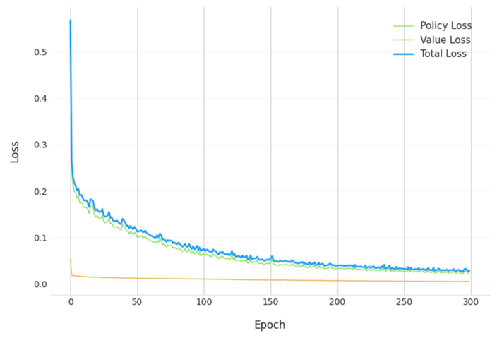
Figure 11 illustrates the loss curves of the TMCTS model over 300 training epochs. The policy network loss converged to 0.0275, the value network loss converged to 0.0046, and the total loss converged to 0.0229. The value network loss decreased rapidly, converging and stabilizing within the first 10 epochs. The policy network loss gradually converged to 0.0275 as training progressed, stabilizing after approximately 250 epochs.
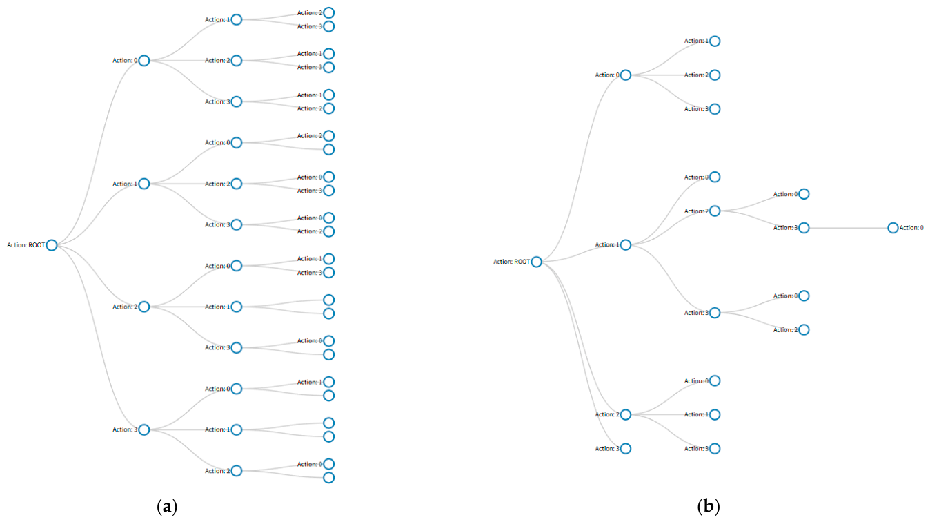
For the ALP, MCTS should prioritize depth-first over breadth-first search logic. The decision tree structure generated by MCTS is illustrated in Figure 12, which depicts the action selection process. A key characteristic of ALP lies in the sequential dependency of decisions: selecting a specific aircraft for landing not only affects the scheduling window of adjacent aircraft but also alters the feasible time intervals for distant aircraft through the propagation of separation constraints. Therefore, the search algorithm must thoroughly explore the complete outcomes of decision sequences. While a breadth-first strategy can evaluate more actions at shallow levels, fully exploring the scheduling sequences of each branch leads to an exponential increase in computational complexity.
The number of MCTS simulations influences both model accuracy and computational time. In this study, MCTS simulations were performed with 32, 64, 128, and 256 iterations. The results obtained for each simulation count, compared against the best-known values (BKV) [30], are presented in Table 3.
As shown in Table 3, when the number of simulations is 128, the average difference reaches −398.298, and the computation time is relatively fast.
On small-sample datasets (first 8 datasets), achieving BKV is possible with 128 simulations, and outperforming BKV occurs in the 8th dataset. When simulations exceed 128, computational results remain unchanged while average computation time increases from 4.234 s to 8.21 s—a 93.9% rise significantly reducing computational efficiency. When the simulation count is below 128, computational efficiency improves only marginally while compromising accuracy. For the eighth dataset, a simulation count of 64 yields a cost of 2025, exceeding the cost of 1860 achieved at 128 simulations.
For large-scale datasets (the last five datasets), the number of simulations substantially affects computation time, which approximately doubles with each doubling of the simulation count. Comparisons indicate that 128 simulations provide both shorter computation times and higher computational accuracy. Therefore, the results obtained with 128 simulations are selected for subsequent comparative analysis.
To verify whether the MCTS-guided reinforcement learning fine-tuning phase can provide incremental gains for pre-trained policies, we compared the performance of T-only (which uses only the Transformer policy head to directly output actions without MCTS) and TMCTS across different-scale cases. The results are presented in Table 4.
The results show that, in large-scale complex scheduling scenarios, TMCTS achieved lower total costs than T-only across all test cases, with an average improvement of 12.01%. This demonstrates that the MCTS-guided RL fine-tuning phase can effectively optimize pre-trained strategies and overcome their performance bottlenecks in large-scale problems.
We compared five algorithms—FCFS, DPALO+GA [29], DPALO+PSO [29], and CPLEX [5]—against the proposed TMCTS approach. The mean interpolation values and average computation times of these algorithms, along with BKV, were calculated on the same dataset. The comparison results are presented in Table 5.
Table 4 demonstrates that the TMCTS approach achieves a significant improvement in average deviation compared to FCFS. Adhering to FCFS under large sample sizes would incur substantial landing costs—specifically, a landing cost of 99,776.58 when handling 500 flights, more than double that of the adjusted methods. Compared to heuristic algorithms DPALO+GA and DPALO+PSO, improvements of 142.938 and 475.755 were achieved, respectively. In terms of computational time, TMCTS achieved a 93.7% improvement over the MIP solver CPLEX, though it still lags behind other algorithms. This is primarily because relying solely on the Transformer’s direct output leads to significant computational inaccuracies. On certain datasets, it may fail to complete the sequencing task, requiring MCTS to search for the optimal ordering sequence. During MCTS simulation, the complexity of the action space and state space grows exponentially. To achieve higher computational accuracy, substantial time is required for MCTS to explore better paths.
When the sample size is less than 50 (first 8 datasets), optimal results can be provided directly. All algorithms achieved the BKV value in the first 7 datasets. For the eighth dataset, the TMCTS computation yielded 1860, outperforming both BKV’s 1950 and previous algorithms while simultaneously ensuring computational accuracy and speed. When the sample size exceeded 100 (the last five datasets), the TMCTS results showed minimal deviation from existing algorithms, maintaining computational accuracy. However, computational efficiency was limited due to algorithmic constraints.

4.2. Discussion

The hybrid learning framework proposed in this paper consists of two stages: behavior cloning pre-training based on genetic algorithm (GA) trajectories, and MCTS-guided reinforcement learning fine-tuning. A potential concern is that, as a stochastic heuristic algorithm, GA may converge to a local optimum, and the trajectory data it generates may impart this “expert bias” to the pre-trained policy. Therefore, it is necessary to verify whether the RL fine-tuning stage can effectively overcome this bias. Theoretically, the UCB formula in the MCTS process encourages the algorithm to actively deviate from the pre-trained prior policy and explore under-visited regions of the action space. When exploratory selections lead to better scheduling outcomes, positive reward signals are backpropagated through the Actor–Critic framework to update the Transformer’s policy network. In terms of experimental evidence, if RL fine-tuning fails to effectively overcome pre-training bias, the performance of TMCTS should not significantly outperform the GA that generated the pre-training data. However, the comparison results in Table 4 show that in Case 8, TMCTS (total cost 1860) outperformed the DPALO+GA results reported in the literature (1863.75); in Case 13, TMCTS (38,629.45) also outperformed DPALO+GA (38,724.21). Furthermore, in Cases 10–12, TMCTS achieved lower total costs than DPALO+GA. These results indicate that MCTS-guided RL fine-tuning successfully guided the agent to explore policy spaces not fully covered by the GA pre-training data, thereby discovering optimal scheduling sequences.
A notable result is evident in the performance of Case 8: the total cost of the TMCTS algorithm proposed in this paper is only 1860, surpassing the known optimal value (BKV) of 1950. Looking at the sequence results, all flights in Case 8 satisfy the minimum separation requirements. The change in cost is due to a shift in the position of Flight 15. Flight 15 has a target landing time of 409, with early arrival and late arrival penalties of 10 each. In the 1950 sequence, Flight 15 lands at 387, with a cost of 220. In the 1860 sequence, Flight 15 is advanced to land at 422, with a cost of 130, reducing the total cost by 90. This also results in the separation matrix violating the triangle inequality (i.e., S1860(25,24) > S1950(25,15) + S1950(15,24)). The structural property that the separation matrix follows the triangle inequality may pose a challenge to classical solution methods (such as CPLEX) that rely on convexity assumptions, and may also mislead certain heuristic algorithms that depend on transitive relationships. The TMCTS algorithm proposed in this paper, based on a Transformer architecture, exhibits stronger robustness to such data anomalies. The multi-head self-attention mechanism enables the model to directly learn and represent dependencies between flights without the need to satisfy assumptions such as the triangle inequality. The MCTS then explores the sequence space based on these learned representations.

5. Conclusions

For the ALP, this paper proposes a deep reinforcement learning method based on MCTS and Transformers. The model outputs the landing sequence and landing times for flights to minimize landing costs. The approach formulates flight scheduling as an MDP and designs a dual-head Transformer network comprising policy and value heads. Leveraging its global attention mechanism, the network captures dependencies among flights and provides prior policy guidance for MCTS. Training is conducted within an Actor–Critic framework, combining behavior cloning pretraining with reinforcement learning optimization.
The experiment utilized the OR-Library dataset. Results indicate that the TMCTS approach achieved a significant improvement in average deviation compared to FCFS, with relative improvements of 142.938 and 475.755 over DPALO+GA and DPALO+PSO, respectively. In terms of computation time, TMCTS achieved a 93.7% improvement over the MIP solver CPLEX, though it remains slower than other benchmark algorithms. The proposed method is able to approximate or outperform known optimal solutions in most cases. However, the number of MCTS simulations constrains the algorithm’s search efficiency. Future improvements could involve expanding training data and extending training time to enhance the quality of the initial policy, thereby reducing the reliance on MCTS simulations and improving overall algorithmic efficiency. The proposed method can assist the AMAN system. First, by statistically analyzing historical flight trajectory information and integrating aircraft performance data with the terminal area route network, it calculates the landing time window (i.e., the earliest and latest possible landing times) for each flight. Second, by receiving real-time flight trajectory data, it computes the landing sequence and timing with the minimum cost for each flight. Compared to traditional rule-based optimization methods, the proposed approach is data-driven and capable of identifying optimization patterns from historical data, resulting in a flight sequence with a lower total cost. This provides new technical support for practical air traffic arrival management and holds significant reference value.
Future improvements could involve expanding the training dataset with more diverse flight scenarios and extending the training epochs to further enhance the quality of the initial policy. This would reduce the reliance on MCTS simulations during inference and improve overall algorithmic efficiency.

Author Contributions

Conceptualization, J.H. and S.Z.; methodology, S.Z. and X.F.; software, J.H. and S.Z.; validation, S.Z., X.F. and X.W.; formal analysis, S.Z.; investigation, S.Z.; resources, J.H., X.F. and X.W.; data curation, S.Z.; writing—original draft preparation, S.Z.; writing—review and editing, J.H., X.F. and X.W.; supervision, X.F. and X.W. All authors have read and agreed to the published version of the manuscript.

Funding

This research was funded by [Jiangsu Province’s Major Science and Technology Project], grant number [BG2025007]; [The State Key Laboratory of Air Traffic Management System], grant number [SKLATM202402]; and the [The National Natural Science Foundation of China], grant number [62173332]. The APC was funded by [Jiangsu Province’s Major Science and Technology Project], grant number [BG2025007].

Data Availability Statement

Publicly available datasets were analyzed in this study. This data can be found here: http://people.brunel.ac.uk/~mastjjb/jeb/orlib/airlandinfo.html (accessed on 11 October 2025).

Conflicts of Interest

The authors declare no conflicts of interest.

References

  1. 2023 Statistical Bulletin on the Development of the Civil Aviation Industry. Available online: http://www.caac.gov.cn/XXGK/XXGK/TJSJ/202505/t20250515_227513.html (accessed on 1 January 2026).
  2. Li, Y.Y. Analysis and Prediction of Airport Delay Based on Big Data Mining. Master’s Thesis, Nanjing University of Aeronautics and Astronautics, Nanjing, China, 2019. [Google Scholar]
  3. Balakrishnan, H.; Chandran, B.G. Algorithms for Scheduling Runway Operations Under Constrained Position Shifting. Oper. Res. 2010, 58, 1650–1665. [Google Scholar] [CrossRef] [Scilit]
  4. Xu, B. An Efficient Ant Colony Algorithm Based on Wake-Vortex Modeling Method for Aircraft Scheduling Problem. J. Comput. Appl. Math. 2017, 317, 157–170. [Google Scholar] [CrossRef] [Scilit]
  5. Girish, B.S. An Efficient Hybrid Particle Swarm Optimization Algorithm in a Rolling Horizon Framework for the Aircraft Landing Problem. Appl. Soft Comput. 2016, 44, 200–221. [Google Scholar] [CrossRef] [Scilit]
  6. Feng, X.R.; Gao, Z.D.; Wang, J.; Wang, X.L.; Hui, K.H. Research on Flight Landing Scheduling Problem Based on Compact Subsequences. J. Beijing Univ. Aeronaut. Astronaut. 2024, 50, 2421–2431. [Google Scholar] [CrossRef]
  7. Beasley, J.E.; Krishnamoorthy, M.; Sharaiha, Y.M.; Abramson, D. Scheduling Aircraft Landings—The Static Case. Transp. Sci. 2000, 34, 180–197. [Google Scholar] [CrossRef] [Scilit]
  8. Beasley, J.E.; Krishnamoorthy, M.; Sharaiha, Y.M.; Abramson, D. Displacement Problem and Dynamically Scheduling Aircraft Landings. J. Oper. Res. Soc. 2004, 55, 54–64. [Google Scholar] [CrossRef] [Scilit]
  9. Pinol, H.; Beasley, J.E. Scatter Search and Bionomic Algorithms for the Aircraft Landing Problem. Eur. J. Oper. Res. 2006, 171, 439–462. [Google Scholar] [CrossRef] [Scilit]
  10. Yu, S.-P.; Cao, X.-B.; Zhang, J. A Real-Time Schedule Method for Aircraft Landing Scheduling Problem Based on Cellular Automation. Appl. Soft Comput. 2011, 11, 3485–3493. [Google Scholar] [CrossRef] [Scilit]
  11. Gui, D.; Le, M.; Luo, X.; Huang, Z. A Metaheuristic Algorithm for Efficient Aircraft Sequencing and Scheduling in Terminal Maneuvering Areas. Optim. Lett. 2025, 19, 579–604. [Google Scholar] [CrossRef] [Scilit]
  12. Pamplona, D.A.; Alves, C.J.P. A Fast Heuristic for Aircraft Landing Scheduling with Time Windows: Application to Guarulhos Airport. Aerospace 2025, 12, 1008. [Google Scholar] [CrossRef] [Scilit]
  13. Chen, X.; Yu, H.; Cao, K.; Zhou, J.; Wei, T.; Hu, S. Uncertainty-Aware Flight Scheduling for Airport Throughput and Flight Delay Optimization. IEEE Trans. Aerosp. Electron. Syst. 2020, 56, 853–862. [Google Scholar] [CrossRef] [Scilit]
  14. Zhang, J.; You, L.; Zhou, M.; Yang, C.; Kang, B. Multi-objective arrival sequencing and scheduling based on point merge system. J. Beijing Univ. Aeronaut. Astronaut. 2021, 49, 66–73. [Google Scholar] [CrossRef]
  15. Wang, J.; Ding, X.; Wang, S. Collaborative Sequencing of Arrival and Departure Aircraft Considering Potential Conflicts. J. Transp. Syst. Eng. Inf. Technol. 2023, 23, 312. [Google Scholar] [CrossRef]
  16. Chen, K.; Situ, T.; Fang, Y. An Improved Multi-Objective Restart Variable Neighborhood Search Algorithm for Aircraft Sequencing Problem with Complex Interdependent Runways. J. Air Transp. Manag. 2025, 127, 102807. [Google Scholar] [CrossRef] [Scilit]
  17. Jiang, H.; Liu, J.X.; Zhou, W.S. Bi-level Programming Model for Joint Scheduling of Arrival and Departure Flights Based on Traffic Scenario. Trans. Nanjing Univ. Aeronaut. Astronaut. 2021, 38, 671–684. [Google Scholar] [CrossRef]
  18. Zhou, D.K. Terminal Area Arrival and Departure Flight Sequencing Based on Reinforcement Learning. Master’s Thesis, Civil Aviation Flight University of China, Guanghan, China, 2024. [Google Scholar]
  19. Kang, R.; Yang, M.; Lin, Z.Y.; Yang, Z.Y. Optimization of Arrival Flight Sequencing Based on EoR Operations. Sci. Technol. Eng. 2025, 25, 8289–8296. [Google Scholar] [CrossRef]
  20. Zhang, C.; Jin, Z.; Ng, K.K.; Tang, T.; Tang, Q. Distributionally robust optimisation approach for aircraft sequencing and scheduling with learning-driven arrival and departure time predictions. Omega 2026, 138, 103415. [Google Scholar] [CrossRef] [Scilit]
  21. Dönmez, K.; Bakır, M.; Cecen, R.K. A Comprehensive Data-Driven MCDM Approach to Determine the Best Single Objective Function for the Aircraft Sequencing and Scheduling Problem. Expert Syst. Appl. 2026, 296, 129172. [Google Scholar] [CrossRef] [Scilit]
  22. Coulom, R. Efficient Selectivity and Backup Operators in Monte-Carlo Tree Search. In Computers and Games; Van Den Herik, H.J., Ciancarini, P., Donkers, H.H.L.M., Eds.; Lecture Notes in Computer Science; Springer: Berlin/Heidelberg, Germany, 2007; Volume 4630, pp. 72–83. ISBN 978-3-540-75537-1. [Google Scholar]
  23. Silver, D.; Huang, A.; Maddison, C.J.; Guez, A.; Sifre, L.; Van Den Driessche, G.; Schrittwieser, J.; Antonoglou, I.; Panneershelvam, V.; Lanctot, M.; et al. Mastering the Game of Go with Deep Neural Networks and Tree Search. Nature 2016, 529, 484–489. [Google Scholar] [CrossRef] [Scilit]
  24. Song, W.S.; Ren, B.Y.; Guan, T. Research on Arch Dam Placement Sequencing Based on Deep Monte Carlo Tree Search. J. Hydroelectr. Eng. 2024, 43, 120–130. [Google Scholar] [CrossRef]
  25. Wang, G.; Pu, H.; Song, T.; Li, W.; Zhang, H.; Hu, G.; Wang, G.; Pu, H.; Song, T.; Li, W.; et al. Integrated Method Based on Reinforcement Learning and Monte Carlo Tree Search for Railway Alignment Optimization. Tiedao Xuebao/J. China Railw. Soc. 2025, 47, 103–110. [Google Scholar]
  26. Peng, J.; Zhu, G.L.; Wu, Q.S.; Li, Y.F.; He, S.; Jin, Y.Y.; Xu, M.L. Scheduling Method for Carrier Aircraft Support Operations Based on Monte Carlo Tree Search. Acta Aeronaut. Astronaut. Sin. 2026, 47, 332444. [Google Scholar] [CrossRef]
  27. Yu, Z.; Huo, M.; Wang, Y.; Wang, S.; Li, Z.; Zhao, Y.; Qi, B.; Qi, N. A UAV Mission Planning Method Based on Improved Monte Carlo Tree Search. J. Astronaut. 2025, 46, 874–883. [Google Scholar] [CrossRef]
  28. Pang, Y.; Zhao, P.; Hu, J.; Liu, Y. Machine Learning-Enhanced Aircraft Landing Scheduling under Uncertainties. Transp. Res. Part C Emerg. Technol. 2024, 158, 104444. [Google Scholar] [CrossRef] [Scilit]
  29. Feng, X.R.; Zhang, S.; Qiu, D.L.; Wang, X.L. A Bounding Optimization Method for Solving Flight Landing Scheduling Problems. J. Nanjing Univ. Aeronaut. Astronaut. 2024, 56, 1024–1035. [Google Scholar] [CrossRef]
  30. Sabar, N.R.; Kendall, G. An Iterated Local Search with Multiple Perturbation Operators and Time Varying Perturbation Strength for the Aircraft Landing Problem. Omega 2015, 56, 88–98. [Google Scholar] [CrossRef] [Scilit]
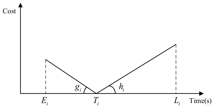
Figure 1. Plot of flight landing time versus cost.
Aerospace 13 00438 g001
Figure 2. Research Framework.
Aerospace 13 00438 g002
Figure 3. Reinforcement learning decision process for flight scheduling.
Aerospace 13 00438 g003
Figure 4. Flowchart of the Dynamic Programming Algorithm.
Aerospace 13 00438 g004
Figure 5. Initial search range.
Aerospace 13 00438 g005
Figure 6. Search range after limit optimization.
Aerospace 13 00438 g006
Figure 7. Algorithm search range.
Aerospace 13 00438 g007
Figure 8. Schematic Diagram of MCTS.
Aerospace 13 00438 g008
Figure 9. Transformer architecture.
Aerospace 13 00438 g009
Figure 10. Actor–Critic Training Framework.
Aerospace 13 00438 g010
Figure 11. Loss of the TMCTS model.
Aerospace 13 00438 g011
Figure 12. Decision tree structure: (a) breadth-first search; (b) depth-first search.
Aerospace 13 00438 g012
Table 1. Wake separation interval(s).
The Aircraft AheadThe Aircraft Behind
HeavyMediumLight
Heavy96157196
Medium6069131
Light606982
Table 2. Parameter settings.
Model ParameterValue
MCTSNumber of simulations128
Exploration constant1.414
Batch search quantity32
TransformerBasic feature dimensions256
Number of attention heads8
Number of encoder stacking layers6
Dropout0.1
Initial learning rate0.0003
Experience replay buffer capacity10,000
Number of training batches128
Table 3. Computational results for different simulation runs.
GroupBKVTMCTS
Num = 32Num = 64Num = 128Num = 256
TCTCt (s)TCt (s)TCt (s)TCt (s)
17007000.757000.9777001.5737002.517
2148014800.35114800.68314801.51114802.804
38208200.4578200.9628201.9198203.677
4252025200.53625200.88425202.03225203.675
5310062600.45131000.88931002.11131003.656
624,44224,4423.11424,4426.30124,44212.84424,44025.559
7155015501.56915503.21415506.686155013.819
8195022851.22120252.49918605.19618609.972
956115907.855.8215861.5111.4235748.7324.8115706.4458.409
1012,32914,142.5811.90213,696.7622.5212,703.5853.38212,793.52119.577
1112,41812,698.9220.69112,675.5439.03512,503.9285.72512,503.92172.669
1216,20917,192.6931.11417,318.3666.42816,725.44121.3616,803.22256.906
1344,83238,134.56145.91838,549.12302.50438,629.45644.30738,444.891221.15
Average difference——13.277——−247.9——−398.298——−403——
Average time————17.22——35.255——74.112——145.722
Average time for the first 8 groups————1.056——2.051——4.234——8.21
Average time for the last 5 groups————43.089——88.382——185.917——365.742
Table 4. Performance comparison between T-only and TMCTS.
GroupT-OnlyTMCTSImprovements
96892.785748.7316.60%
1018,060.0012,703.5829.66%
1113,417.1612,503.586.81%
1217,594.7216,725.444.94%
1339,435.0438,629.452.04%
Average19,079.9417,262.2212.01%
Table 5. Comparison of results from various algorithms.
GroupBKVFCFSTMCTSDPALO+GADPALO+PSOCPLEX
TCt (s)TCt (s)TCt (s)TCt (s)
170012807001.5737000.0047000.0067000.8
21480179014801.51114800.02814820.04614800.8
382017908201.9198200.0258200.0588201.3
42520489025202.03225200.00425200.00625202.3
53100647031002.11131000.04332440.15931003.7
624,44224,44224,44212.84424,4420.00424,4420.00624,4420.7
71550155015506.68615500.00515500.00715501.2
8195018,87018605.1961863.750.0561863.250.18519502.2
9561118,937.165748.7324.8115694.522.5415675.013.2235611.7932.2
1012,32927,66012,703.5853.38213,826.425.72714,799.944.61512,292.23600
1112,41835,532.9112,503.9285.72512,671.364.70612,922.425.50612,418.33600
1216,20946,471.7216,725.44121.3617,249.116.7217,626.096.84916,122.23600
1344,83299,776.5838,629.45644.30738,724.2121.9141,323.2312.05237,848.93600
Average difference——12,423.03−398.298——−255.36——77.457——−546.6——
Average time——————74.112——3.214——2.517——1180.4
Disclaimer/Publisher’s Note: The statements, opinions and data contained in all publications are solely those of the individual author(s) and contributor(s) and not of MDPI and/or the editor(s). MDPI and/or the editor(s) disclaim responsibility for any injury to people or property resulting from any ideas, methods, instructions or products referred to in the content.