Aerodynamic Optimization of a Folding Tandem-Wing UAV: Parameter Interaction Analysis and Surrogate Modeling

Abstract

Folding-wing Unmanned Aerial Vehicles (UAVs) have become a key platform in modern aerial applications, owing to their superior portability and rapid deployment capabilities. While the tandem-wing configuration offers a compact solution for strict folding constraints, the resulting high wing loading necessitates a maximized lift coefficient (C_L) to ensure efficient low-speed loitering. This study presents an aerodynamic optimization framework aiming to maximize the C_L of a folding tandem-wing UAV. A combined optimization strategy integrating Optimal Latin Hypercube Sampling (OLHS), orthogonal polynomial surrogate models, and the Multi-Island Genetic Algorithm (MIGA) is established. With aft wing parameters determined, global sensitivity analysis identifies the fore wing span as the dominant factor, contributing 47.40% to lift performance. Crucially, although vertical separation contributes only 6.53% to C_L and sweep angle just −1.22% to drag coefficient, their strong interaction effects with wing span confirm their non-negligible role. Finally, the flow field characteristics at the wing root of the optimized configuration undergo significant changes, resulting in a 4.28% increase in the C_L. This work validates the important role of parameter interaction effects in aerodynamic optimization and provides a theoretical basis for the design of geometrically constrained aerial vehicles requiring high lift coefficients.

1. Introduction

In recent years, small-scale folding-wing Unmanned Aerial Vehicles (UAVs) have gained significant attention in fields such as remote sensing, environmental monitoring, and emergency rescue due to their portability and rapid deployment capabilities [1]. Unlike conventional fixed-wing aircraft, these platforms are often required to loiter in a specific area for extended periods to perform continuous data acquisition tasks. To maximize operational flexibility and portability, these platforms are often designed with tube-launched capabilities, necessitating compact, foldable aerodynamic configurations that can deploy rapidly post-launch. Integrating sufficient payloads within such geometrically restricted configurations imposes higher demands on their aerodynamic lift capacity to ensure effective loitering. Among various configurations, the tandem-wing layout—characterized by fore and aft wings—has been widely favored for its ability to provide sufficient lift within a constrained span while maintaining longitudinal stability under varying center-of-gravity conditions.

The theoretical foundation for tandem-wing aerodynamics traces back to the pioneering works of Munk [2] and Prandtl [3], who established that multi-surface configurations could minimize induced drag and enhance lift capacity through optimal load distribution. Specifically, for folding tandem-wing UAVs, flight operations typically occur in a low Reynolds number regime (Re = 10⁴–10⁵). As highlighted by Jones et al. [4] and Zhang et al. [5], the flow field in this domain is dominated by boundary layer characteristics and transition phenomena, rendering the aerodynamic performance highly sensitive to geometric variations. Within this context, the aerodynamic interference between the fore and aft wings becomes the governing factor. Early experimental studies by Scharpf and Mueller [6] and Broering [7] verified that the relative positioning—specifically vertical and horizontal separation—drastically alters the downwash field and wake trajectory, thereby determining the lift-to-drag ratio. Cai et al. [8] and Delikan et al. [9] further quantified these interference effects through numerical simulations, demonstrating that improper wing separation can lead to severe performance penalties. In terms of flow interference mechanisms and theoretical modeling, Shah and Ahmed [10] analyzed the secondary stall mechanism induced by the downstream wing suppressing the vortex shedding of the upstream wing, while Cheng et al. [11] refined prediction models based on lifting-line theory to better capture these interactions. Additionally, Figat and Kwiek [12] emphasized that the longitudinal dynamic stability of tandem layouts under varying flight conditions is strongly influenced by aerodynamic coupling. Despite extensive analyses on flow physics, stability characteristics, and other relevant aspects in existing studies [13,14], there remains a lack of systematic geometric parameter optimization schemes specifically aimed at performance enhancement under strict dimensional constraints. Furthermore, as noted by Kostić et al. [15] and Shi et al. [16], the multi-parameter design space of tandem wings exhibits complex coupling relationships, and it is difficult to efficiently grasp the global laws merely through single-parameter analysis and Computational Fluid Dynamics (CFD) calculations. Therefore, it is necessary to adopt targeted optimization strategies to improve the efficiency and accuracy of design optimization.

To address the challenge of prohibitive computational costs associated with high-fidelity CFD simulations in multi-parameter design spaces, Surrogate-Based Optimization (SBO) has evolved into a standard methodology in aeronautical engineering. Existing studies have explicitly clarified the efficacy of SBO strategies in improving optimization efficiency by replacing expensive numerical simulations with mathematical approximations [17]. The selection of appropriate surrogate models is critical. Simpson et al. [18] and Forrester et al. [19] developed theoretical frameworks for model selection, highlighting the trade-offs between accuracy and computational expense. Regarding model types, Han et al. [20] validated the capability of advanced Kriging strategies in accurately modeling complex global aerodynamic landscapes, while Krishnamurthy [21] verified the effectiveness of the augmented and compactly supported Radial Basis Function (RBF) in local response surface construction. Furthermore, Giunta and Watson [22] provided comparative insights between polynomial response surfaces and interpolation models, offering guidance for engineering applications. To ensure the prediction fidelity of these models with limited computational resources, efficient sampling strategies are indispensable. Latin Hypercube Sampling (LHS), as originally established by McKay et al. [23], serves as the fundamental benchmark for space-filling designs due to its efficient stratification properties. Building upon this foundational mechanism, Optimal Latin Hypercube Sampling (OLHS) further enhances spatial uniformity by mathematically optimizing the inter-site distances to effectively prevent sample clustering. However, to effectively locate the global optimum within the surrogate-predicted landscape, it is necessary to introduce a robust evolutionary algorithm to drive the search process.

In terms of global search algorithms coupled with surrogates, the Genetic Algorithm (GA), originally proposed by Holland [24], serves as a foundational evolutionary strategy. Gong and Gu [25] successfully applied GA to Multidisciplinary Design Optimization (MDO) systems, validating their robustness in addressing nonlinear and coupled non-convex problems. Yan et al. [26] introduced machine learning techniques into aerodynamic shape optimizers, further pushing the boundaries of design automation. These advanced SBO frameworks have been successfully implemented in various complex aerodynamic designs: Zhang et al. [27] achieved efficient shape optimization for hypersonic lifting bodies, and Liang et al. [28] conducted robust multi-objective design for wing planforms. Addressing complex flow control challenges, Du et al. [29] optimized a high-lift configuration with circulation control, further verifying the capability of SBO strategies in capturing strong aerodynamic nonlinearities. Furthermore, Gong and Ma [30] performed shape optimization and sensitivity analysis for morphing-wing aircraft, demonstrating the method’s capability in handling variable geometric configurations. Additionally, Qian et al. [31] emphasized the importance of building surrogates based on detailed simulations to ensure engineering validity. Collectively, these established methodologies provide a solid theoretical foundation for solving complex aerodynamic optimization problems.

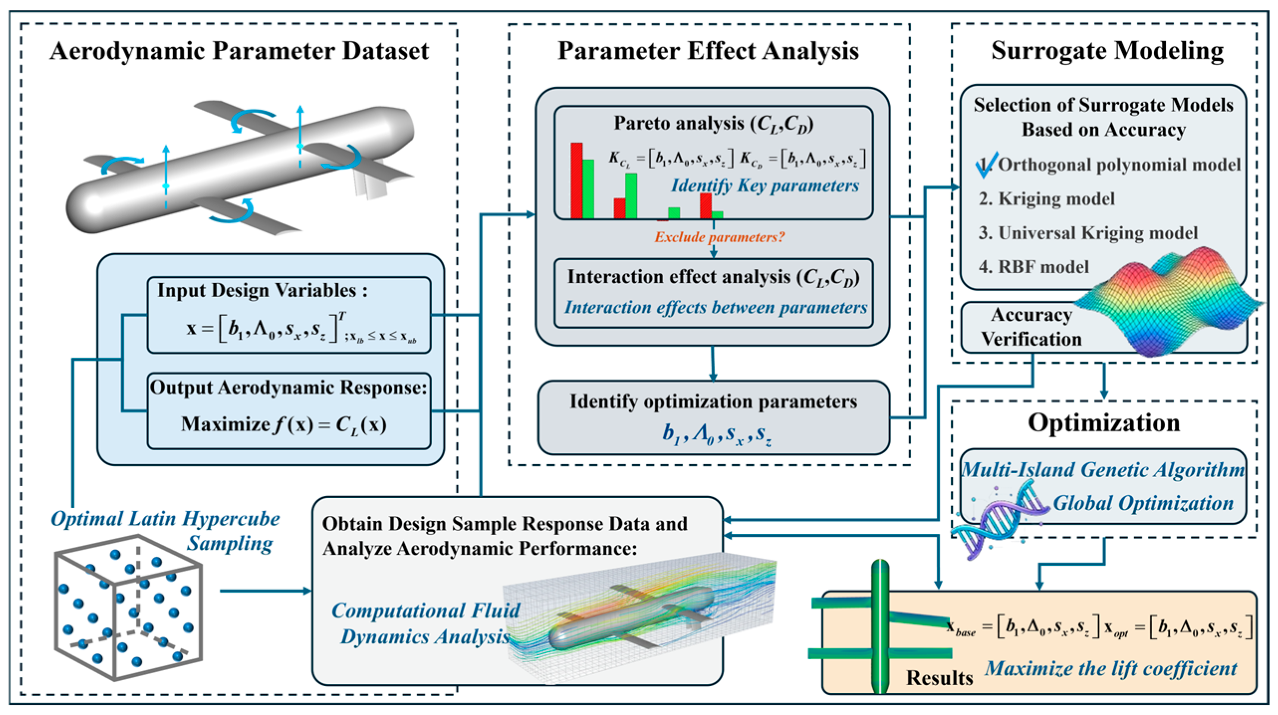
However, despite these extensive applications in aviation, the application of systematic SBO frameworks specifically to folding tandem-wing UAVs remains relatively limited. Most existing studies focus on single-element wings or conventional layouts, often neglecting the complex aerodynamic coupling unique to tandem configurations under strict geometric constraints. Therefore, this study integrates OLHS with a Multi-Island Genetic Algorithm (MIGA) to construct a high-precision aerodynamic optimization framework. By systematically analyzing the mapping relationship between geometric parameters and aerodynamic characteristics, this approach aims to efficiently identify the optimal configuration that maximizes lift capability under strict tube-launch folding constraints. The overall technical route and research methodology adopted in this paper are schematically illustrated in Figure 1. The remainder of this paper is organized as follows: Section 2 details the geometric configuration of the folding tandem-wing UAV and the numerical simulation methods used for aerodynamic analysis. Section 3 elaborates on the surrogate-based optimization strategy, including the experimental design, parameter sensitivity analysis, and the discussion of optimization results. Finally, Section 4 summarizes the key findings and conclusions of this study.

2. Models and Numerical Simulation

2.1. Configuration and Baseline Design

The geometric model of the folding tandem-wing UAV established in this study is based on the design of a representative tandem-wing system reported in the open literature [32]. To meet the design requirements of individual portability and tube-launch capability, the UAV utilizes a high-aspect-ratio cylindrical fuselage integrated with a folding tandem-wing and twin vertical tail configuration. This design ensures efficient payload space utilization while achieving compact storage before launch and rapid deployment post-launch, balancing structural compactness with aerodynamic efficiency [33].

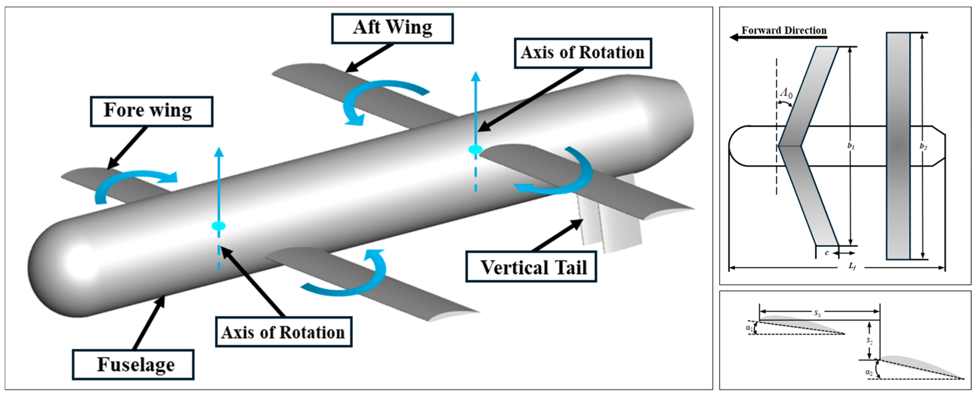
The UAV primarily operates in a low Reynolds number environment; therefore, the NACA 6409 airfoil, known for its favorable low-speed stall characteristics, is selected for both fore and aft wings [34]. Regarding the aerodynamic layout, a vertical stagger configuration with a “low-placed fore wing and high-placed aft wing” is adopted. This provides necessary clearance for the longitudinal rotation of the fuselage and nose during the transition from folding to deployment, preventing mechanical interference inside the canister. Aerodynamically, this vertical stagger ensures that the fore wing stalls before the aft wing, generating a nose-down restoring moment that guarantees longitudinal stability. The geometry and component illustrations are shown in Figure 2.

The aerodynamic performance of the tandem-wing configuration is highly sensitive to the relative arrangement of the wing surfaces. With reference to the design method proposed by Wang et al. [35], to simplify the design process and mitigate the complexity of parameter coupling, the design parameters of the aft wing were initially fixed. Subsequently, four key geometric parameters were defined to describe the configuration: fore wing span (b₁), fore wing sweep angle (Λ₀), horizontal separation (s_x), and vertical separation (s_z) between the fore wing and aft wing, as illustrated in Figure 2. The verification configuration, as the initial design scheme for verifying the rationality and reliability of the numerical solution method, has its parameters summarized in

Table 1. Geometric Parameters of the UAV.

Parameter	Verification Configuration	Bounds
Fuselage Length (Lf)	2.200 m	-
Chord Length (c)	0.186 m	-
Angle of Attack (AOA)	4°	-
Aft Wing Span (b2)	2.518 m	-
Fore Wing Span (b1)	1.916 m	7.4c–13.4c
Fore Wing Sweep Angle (Λ0)	0°	0°–6°
Horizontal Separation between Fore and Aft wings (sx)	0.940 m	2c–6c
Vertical Separation between Fore and Aft Wings (sz)	0.093 m	−0.2c–0.8c

. It is worth noting that, due to constraints imposed by structural dimensions and the folding mechanism, the physically feasible ranges of these geometric parameters are strictly limited. These constraints define the practical design boundaries for the subsequent aerodynamic optimization.

2.2. Governing Equations and Solution

CFD simulations are employed to obtain design sample response data and analyze aerodynamic performance. The core solution objective is the steady-state incompressible Reynolds-averaged Navier–Stokes (RANS) equations [36], which aim to capture boundary layer evolution and flow field characteristics over the wing surface. For steady incompressible flow, the governing equations comprise the mass conservation equation and the momentum conservation equation, expressed as (1) and (2). Key flow conditions set during the solution process, tailored to the cruise flight conditions of the UAV, are as follows: The free stream velocity V = 30 m/s is determined based on the design cruise speed, with Reynolds number Re ≈ 3.70 × 10⁵. Velocity Inlet and Pressure Outlet boundary conditions are applied. Non-slip wall conditions were applied to the surfaces of the leading edge, trailing edge, and fuselage to accurately simulate viscous flow near the wall and boundary layer development. Given the symmetric nature of the flow field during cruise conditions, a half-model computational approach was adopted to enhance computational efficiency in solving the flow field.

Mass Conservation Equation:

$${\displaystyle \frac{\partial {\overline{u}}_i}{\partial x_i}}=0$$

(1)

Momentum Conservation Equation:

$$\rho {\overline{u}}_j{\displaystyle \frac{\partial {\overline{u}}_i}{\partial x_j}}=-{\displaystyle \frac{\partial \overline{p}}{\partial x_i}}+{\displaystyle \frac{\partial }{\partial x_j}}\left(\mu {\displaystyle \frac{\partial {\overline{u}}_i}{\partial x_j}}-\rho \overline{{u^{\prime }}_i{u^{\prime }}_j}\right)$$

(2)

where ${\overline{u}}_i$ and ${\overline{u}}_j$ are time-averaged velocity components, $\overline{p}$ is time-averaged pressure, $\rho$ is fluid density, $\mu$ is dynamic viscosity, and $-\rho \overline{u_i^{\mathrm{\prime }}{u}_j^{\mathrm{\prime }}}$ is the Reynolds stress, representing the effect of turbulent fluctuations on the mean flow field. This term is closed by introducing a turbulence model.

To balance numerical simulation accuracy and efficiency, the Shear Stress Transport (SST) k-ω turbulence model is selected [37]. This model combines the near-wall precision of the k-ω model with the far-field stability of the k-ε model, enabling accurate capture of flow field variations and boundary layer separation. The convective term in the governing equations is discretized using a Second-Order Upwind Scheme to enhance computational accuracy in regions with high flow gradients. The diffusion term is discretized using a central differencing scheme to ensure conservation in numerical discretization. The SIMPLE algorithm is adopted for pressure-velocity coupling. Through the iterative solution of the pressure correction equation and momentum equations, this method effectively ensures pressure-velocity consistency in incompressible flow fields, enhancing computational convergence stability.

2.3. Verification and Validation

2.3.1. Grid Independence Verification

To minimize the influence of grid quantity on simulation results and eliminate numerical errors caused by discretization, a grid independence study was conducted. The objective was to select a meshing scheme that balances low numerical error with high computational efficiency for subsequent simulations. The first layer height of the grid near the wall was set to 0.02 mm, to ensure Y⁺ ≈ 1. Three sets of unstructured grids, ranging from coarse to fine, were generated using the method proposed by Wang et al. [38]. The total cell counts for the three grids were 2.51 million, 3.56 million, and 4.88 million, respectively. Under the cruise condition, the lift coefficient (C_L) of the UAV was calculated using these three grid sets, with the results summarized in

Table 2. Grid Independence Verification.

Grid Cells	Lift Coefficient (CL)	CL Deviation
2.51 million	0.569	-
3.56 million	0.577	1.41%
4.88 million	0.582	0.87%

.

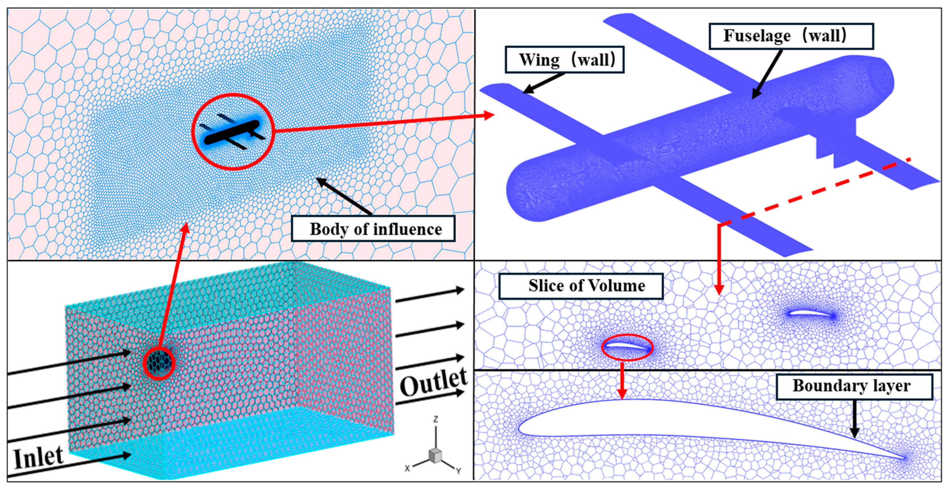
At a grid size of 3.56 million, the deviation in C_L relative to the refined 4.88 million grid is only 0.87%, which satisfies engineering accuracy requirements. Therefore, considering the trade-off between computational accuracy and cost, the 3.56 million cell grid scheme (flow field mesh details are shown in Figure 3) was selected for the subsequent automated solution process.

2.3.2. Experimental Validation

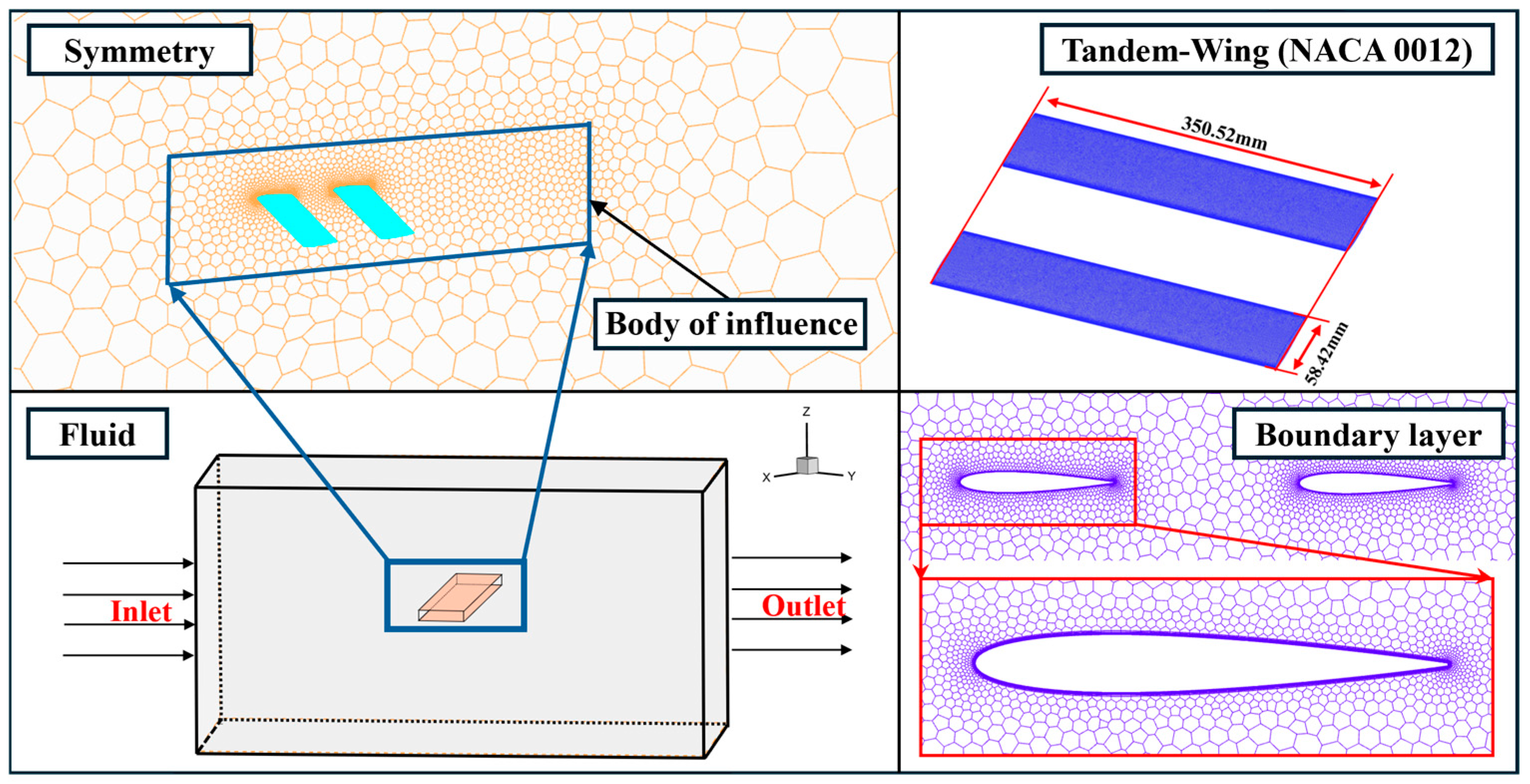
To ensure the reliability of the numerical method, the CFD results were validated against the wind tunnel experimental data of a tandem-wing configuration. The experiment conducted by Shah [39] on NACA 0012 tandem wings was selected as the benchmark case to verify the accuracy of the adopted numerical calculation method. This experiment specifically investigated the aerodynamic coupling effects by varying the fore wing incidence angle (φ) while keeping the aft wing fixed, which is consistent with the research in this paper. Numerical settings strictly followed the experimental parameters (listed in

Table 3. Parameters of the Validation Model.

Parameter	Value
Chord Length (c)	58.42 mm
Aspect Ratio (AR)	6
Free-stream Velocity (V)	25 m/s
Fore wing incidence angle (φ)	0°–10°
Reynolds Number (Re)	1.00 × 105
Density (ρ)	1.225 kg/m3
Dynamic viscosity (μ)	1.789 × 10−5 Pa·s

), utilizing the SST k-ω model and ensuring Y⁺ ≈ 1 near the wall, which guarantees the accuracy of the near-wall flow simulation. The Reynolds number is 1.0 × 10⁵, which lies within the same low-Reynolds-number regime as the target UAV (Re ≈ 3.7 × 10⁵), ensuring the similarity of flow characteristics between the two. The validation grid details are shown in Figure 4.

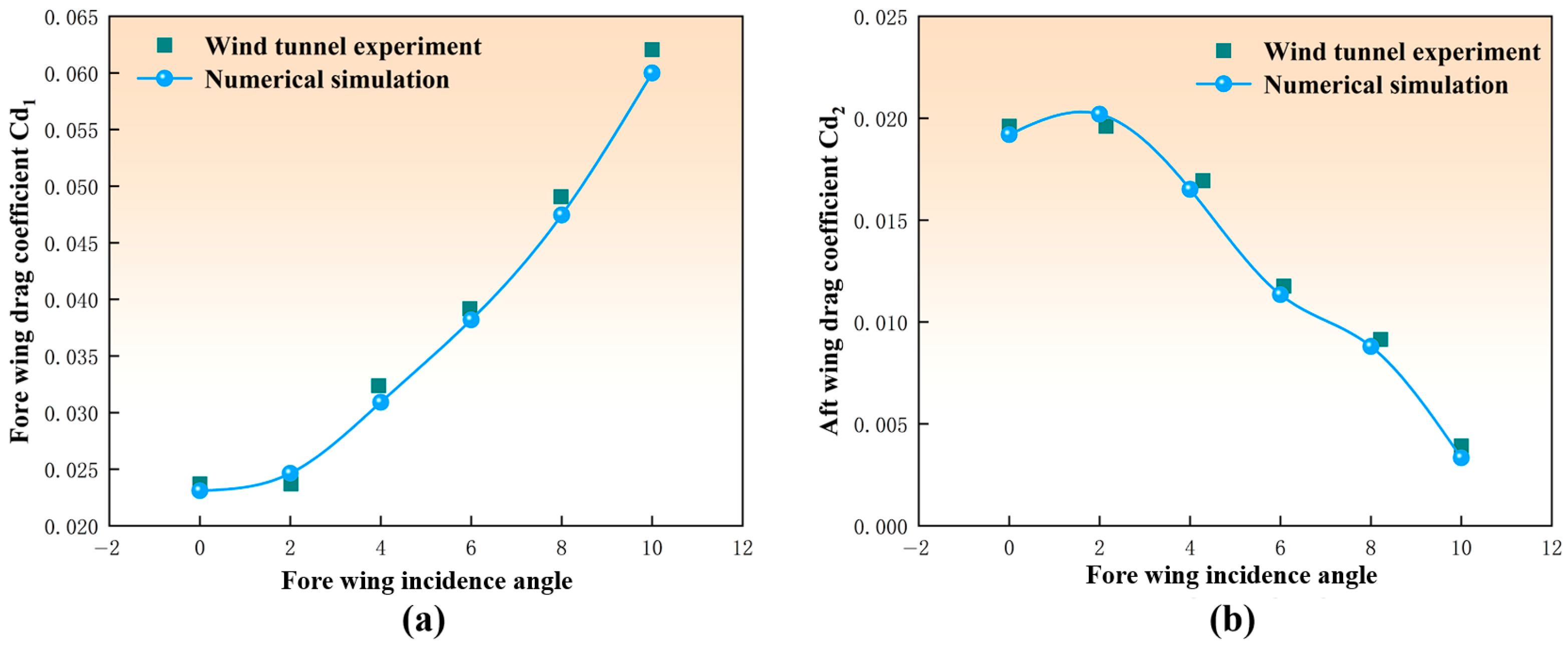
Considering the complex aerodynamic coupling between the fore and aft wings of the tandem configuration, it is necessary to separately validate the simulation results of the fore and aft wings, as shown in Figure 5. The comparative analysis reveals good agreement between the numerical simulation results in this study and the wind tunnel experimental data from Shah, S.H.R. [39]. The deviation in the drag coefficient between the wings, when varying the fore wing incidence angle, is within 5%, which meets the engineering accuracy requirements.

It is well recognized in low-Reynolds-number aerodynamics that drag coefficient prediction is inherently more sensitive to numerical setup and flow conditions than lift coefficient. Therefore, achieving a drag coefficient deviation within 5% between CFD and experimental data (as shown in Figure 5) provides strong evidence that the numerical framework accurately captures not only the primary lift characteristics but also the more delicate drag-related flow physics, including boundary layer development and wake interference. This level of agreement confirms the overall reliability of the aerodynamic simulations for the tandem-wing configuration.

3. Optimization Framework and Strategy

3.1. Optimization Problem Definition

To enhance the aerodynamic efficiency and payload capacity of the folding UAV, the design task is formulated as a constrained non-linear programming problem. Based on the geometric characteristics and physical constraints described in Section 2.1, the four key parameters governing the tandem-wing configuration are selected as the design variables.

Let $\mathrm{x}\in {\mathrm{R}}^4$ be the design vector defined as:

$$x={\left[b_1,{\Lambda }_0,s_x,s_z\right]}^T$$

(3)

where b₁ represents the fore wing span, Λ₀ is the fore wing sweep angle, s_x and s_z denote the horizontal and vertical separations between the tandem wings. The search space for these variables is strictly confined by geometric constraints to ensure the feasibility of the folding mechanism and compatibility with the launch canister. These physical limitations, as detailed in Table 1, are translated into mathematical side constraints (i.e., upper and lower bounds):

$$\begin{array}{cc}\mathrm{Fore} \mathrm{wing} \mathrm{span},& b_1: 7.4\mathrm{c} \le b_1 \le 13.4\mathrm{c}\\ \mathrm{Fore} \mathrm{wing} \mathrm{sweep} \mathrm{angle},& {\Lambda }_0: 0° \le {\Lambda }_0 \le 6°\\ \mathrm{Horizontal} \mathrm{separation},& s_x: 2\mathrm{c} \le s_x \le 6\mathrm{c}\\ \mathrm{Vertical} \mathrm{separation},& s_z: -0.2\mathrm{c} \le s_z \le 0.8\mathrm{c}\end{array}$$

It should be emphasized that the wing reference area is not set as an independent design variable. Instead, it is determined by the geometric layout parameters, which are strictly bounded by the folding mechanism and launch canister constraints listed in Table 1. The fore wing span is constrained by 7.4 ≤ b₁ ≤ 13.4c, and the aft wing span is fixed at 2.518 m. These constraints ensure that the total wing area varies within a very narrow range.

The definition of the optimization objective is strictly driven by the unique flight profile and geometric constraints of the folding tandem-wing UAV. Unlike conventional cruise UAVs where the lift-to-drag ratio (L/D) is maximized for range, this platform faces a specific challenge: the strict span limit imposed by the launch canister, combined with the requirement for a high-density payload (e.g., optical pods or long-endurance batteries), results in a significantly high wing loading (W/S) [1]. According to the stall speed equation V_stall (Equation (4)), increasing the C_L is the primary aerodynamic means to lower the minimum flight speed without compromising payload capacity. This not only expands the low-speed flight envelope for extended observation missions but also provides a critical lift margin for agile maneuvers during complex flight phases, preventing accelerated stall (Equation (5)). Consequently, this study defines the maximization of the C_L as the primary optimization objective.

$$V_{stall}=\sqrt{{\displaystyle \frac{2W}{\rho S{C}_{L,max}}}}$$

(4)

$$n_{max}={\displaystyle \frac{\frac{1}{2}\rho V^{2}S{C}_{L,max}}{W}}$$

(5)

Based on the above definitions, the mathematical model of the aerodynamic optimization problem is established as follows:

$$\left\{\begin{array}{l}\mathrm{Find} x={\left[b_1,{\Lambda }_0,s_x,s_z\right]}^T\hfill \\ \mathrm{Maximize} f(x)=C_L(x)\hfill \\ \mathrm{Subject} \mathrm{to} x_{lb}\le x\le x_{ub}\hfill \end{array}\right.$$

(6)

where C_L(x) is the lift coefficient predicted by the surrogate model (detailed in Section 3.3), and x_lb and x_ub represent the lower and upper bounds of the design variables, respectively, ensuring the optimized geometry remains within the manufacturable and deployable limits.

3.2. Surrogate-Based Optimization Methodology

3.2.1. Optimal Latin Hypercube Sampling

The quality of the surrogate model is critically dependent on the spatial distribution of the training samples [40]. To accurately capture the aerodynamic nonlinearities across the design space, the Design of Experiments (DOE) is performed using the OLHS method.

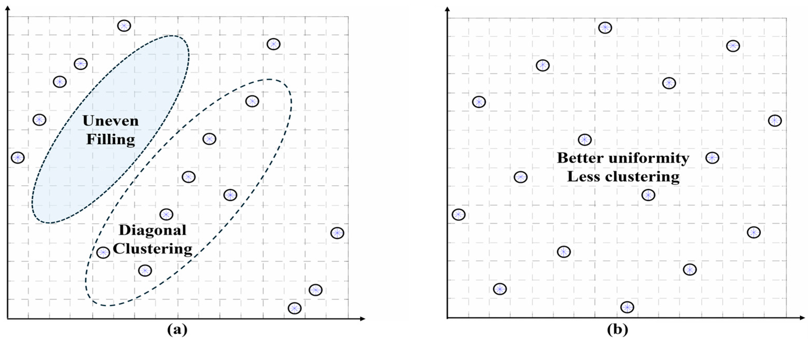
The fundamental principle of standard LHS [23] operates within an m-dimensional design space. The range of each design variable $x_k\left(k\in [1,m]\right)$, denoted as $[x_k^{min},x_k^{max}]$, is divided into n uniform sub-intervals, with the i-th sub-interval denoted as $\left[x_k^{i-1},x_k^i\right]\left(i\in [1,n]\right)$. Subsequently, n sample points are randomly selected such that each sub-interval of every factor contains exactly one sample. However, due to this random selection process, standard LHS often suffers from uneven spatial filling or diagonal clustering, as illustrated in Figure 6, which can degrade the prediction accuracy in sparse regions.

In contrast, OLHS introduces an optimization adjustment stage [41] upon the LHS framework. While retaining the constraint that each sub-interval $\left[x_k^{i-1},x_k^i\right]$ for every dimension must contain strictly one sample point, OLHS employs an optimization algorithm to iteratively adjust the positions of these points. This process aims to satisfy specific optimality criteria, typically maximizing the minimum Euclidean Distance between sample points, thereby achieving optimal spatial coverage [42]. Consequently, as shown in Figure 6, OLHS constructs an m-dimensional sampling space that achieves both superior multidimensional uniformity and statistical independence, ensuring robust coverage of the design space.

Considering that the flow field of a tandem-wing configuration is characterized by complex vortex interference and strong non-linearities [14], a sufficient sample size (N) is required to accurately capture the response landscape. To ensure high prediction fidelity and prevent under-fitting in regions with steep gradients, a robust sampling strategy is adopted. Consequently, a total of 70 sample points are generated. This sample size is selected to strike an optimal balance between computational cost and modeling accuracy, providing a robust and dense coverage of the four-dimensional design space.

3.2.2. Surrogate Model Construction and Accuracy

The core of the surrogate model lies in fitting the mapping relationship between design inputs and output responses via mathematical modeling methods. By replacing computationally expensive CFD simulations, it enables efficient exploration of the design space during the iterative optimization process. Due to the complex nonlinear nature of the flow field, no single surrogate model is universally superior for all aerodynamic responses. Therefore, to identify the suitable predictor for the UAV, four representative surrogate models are evaluated: Orthogonal Polynomials [43], Kriging [44], Universal Kriging [45], and Radial Basis Functions (RBF) [46].

The Orthogonal Polynomial Model approximates the response y(x) using a linear combination of basis functions:

$$\widehat{y}(x)={\displaystyle \sum _{j=1}^K{\beta }_j}{\varphi }_j(x)$$

(7)

where ${\beta }_j$ are the regression coefficients determined by least squares, and ${\varphi }_j$ are orthogonal basis functions suitable for capturing global quadratic trends.

The RBF Model constructs the approximation based on the Euclidean Distance from sample points:

$$\widehat{y}(x)={\displaystyle \sum _{i=1}^N{w}_i}\psi \left(\Vert x-x_i\Vert \right)$$

(8)

where $\psi$ is the basis function (e.g., Gaussian or Multiquadric) and w_i are weight coefficients. This method is particularly effective for highly nonlinear landscapes.

Additionally, Kriging and Universal Kriging models are based on Gaussian process regression (GPR) [20], treating the response as a combination of a global trend and a local stochastic deviation.

The accuracy of these models is assessed using a strictly independent validation strategy. Based on the OLHS method described in Section 3.2.1, a training set consisting of 70 samples is generated to construct the surrogates. Additionally, a separate validation set of 8 independent samples is generated to test the generalization capability of the models. The Coefficient of Determination (R²) and Root Mean Square Error (RMSE) are adopted as the evaluation metrics.

Table 4. Comparison of Surrogate Model Accuracy.

Surrogate Model	CL		CD
	R2	RMSE	R2	RMSE
Orthogonal polynomial model	0.8884	0.0962	0.5460	0.2193
Kriging model	0.8767	0.1140	0.7247	0.1892
Universal Kriging model	0.7831	0.1512	0.6811	0.2036
RBF model	0.8532	0.1241	0.7816	0.1685

presents the comparison of prediction accuracy among the four models. The results reveal distinct performance characteristics for different aerodynamic objectives.

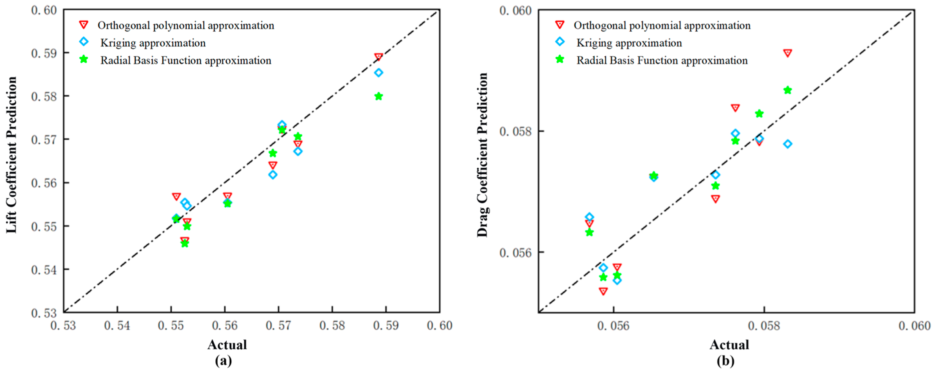
While the RBF Model proves superior for the drag coefficient (C_D) with an R² of 0.7816 due to its ability to interpolate complex local non-linearities, the Orthogonal Polynomial Model demonstrates the highest fidelity for C_L, achieving an R² of 0.8884 and an RMSE of 0.0962. This indicates that the lift variation within the design space is dominated by second-order global trends efficiently captured by polynomial functions. The selection of the OPM is based on a holistic evaluation of both predictive accuracy and global stability. While other models such as Kriging exhibit only a relatively small difference in prediction accuracy compared to the OPM, the OPM is inherently superior in capturing the global trends of the design space and the relationships between the geometric parameters and aerodynamic responses. This ensures more stable and reliable predictions across the entire optimization domain, which is critical for the robustness of the optimization framework, especially when navigating the complex design space of the folding tandem-wing UAV. To visually verify the prediction fidelity, the C_L values predicted by the three types of surrogate models with better accuracy are plotted against the actual CFD validation data in Figure 7. As observed in the plot, the data points for the Orthogonal Polynomial Model are tightly clustered around the diagonal line, indicating superior agreement. Although the subsequent optimization focuses on lift maximization to ensure flight feasibility, the successful modeling of the highly non-linear drag characteristics serves as a rigorous verification of the proposed DOE framework. It confirms that the OLHS strategy provides sufficient coverage of the complex flow field, thereby reinforcing confidence in the reliability of the primary lift model. Consequently, the Orthogonal Polynomial Model is selected as the surrogate driver for the optimization.

3.2.3. Multi-Island Genetic Algorithm

Based on the established high-fidelity surrogate model, the global search for the optimal geometric parameters is conducted using the Multi-Island Genetic Algorithm (MIGA). The aerodynamic design space of the tandem-wing configuration typically exhibits high non-linearity and multiple local optima due to complex wing interference. Traditional gradient-based methods or Standard Genetic Algorithms (SGA) are often prone to premature convergence in such landscapes [25]. MIGA addresses this by introducing a distributed population structure. Unlike SGA, MIGA divides the total population into several sub-populations, termed “islands”. Evolution operations are performed independently within each island, and a migration operation periodically transfers individuals between them to maintain genetic diversity. The specific configuration parameters governing these operations are detailed in

Table 5. Configuration Parameters of MIGA.

Parameter	Value
Population Size	10
Number of Islands	4
Evolution Generations	80
Crossover Probability	0.8
Mutation Probability	0.02
Inter-Island Migration Rate	0.2
Migration Interval Generations	5

. Selected to balance exploration robustness and computational cost, the algorithm is configured with 4 islands, a migration rate of 0.2, and a total evolution of 80 generations.

To further enhance the optimization efficiency, a population seeding strategy is adopted. Instead of starting with a completely random population, the initial generation is seeded with the top 10 elite individuals screened from the OLHS dataset (Section 3.2.1). During the evolutionary process, the fitness of each individual is evaluated using the constructed Orthogonal Polynomial Model. This combined optimization strategy circumvents the prohibitive computational costs of repetitive calculations, ensuring that the global search remains both efficient and feasible.

3.3. Parameter Sensitivity Analysis

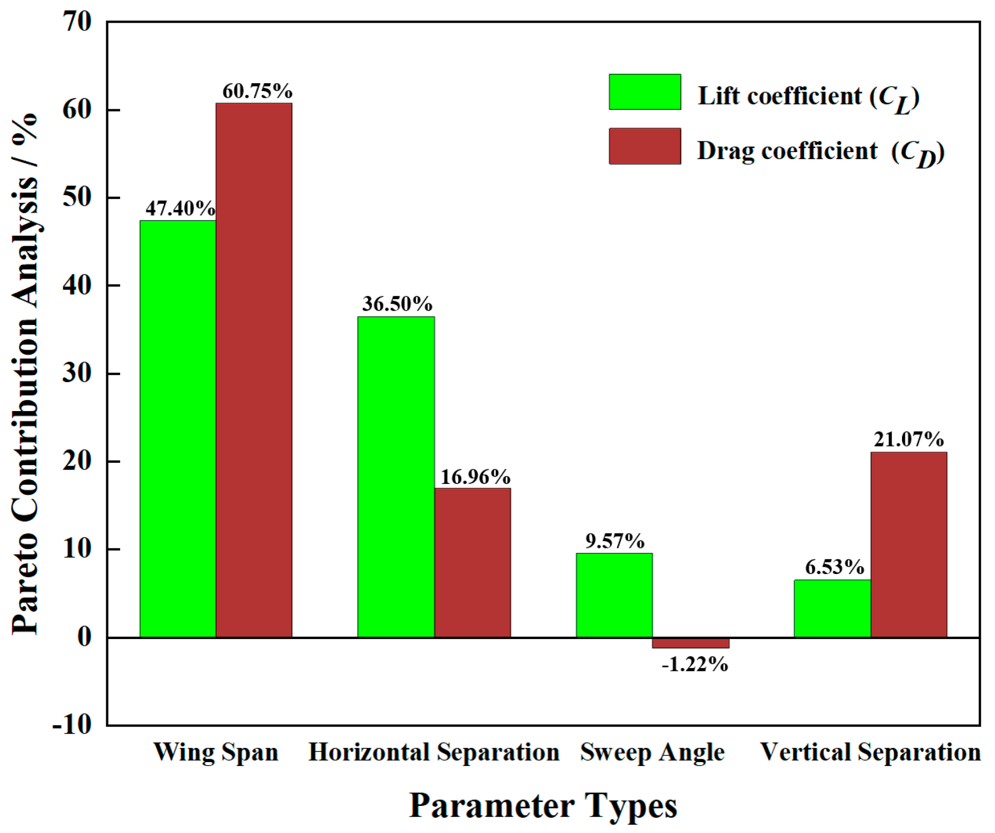
To ensure the effectiveness of the global optimization, it is essential to rigorously evaluate the influence of the design variables before executing the MIGA. The primary objective of this sensitivity analysis is not merely to analyze parameter contributions and clarify the optimization direction, but also to validate the necessity of the selected design space. Specifically, it aims to determine whether parameters with low apparent contribution should be excluded to simplify the model, or retained due to potential interaction effects. Based on the OLHS dataset, the Pareto contribution analysis quantifies the relative sensitivity of the aerodynamic characteristics to variations in the design parameters, as illustrated in Figure 8.

Focusing first on the C_L, the b₁ exhibits the most significant relative positive influence, accounting for approximately 47.40% of the total variation. The lift of a traditional single-wing configuration is primarily influenced by the lift area, whereas a tandem-wing configuration operates differently. In this study, the Λ₀ contributes 9.57%, the s_z accounts for 6.53%, while the s_x accounts for 36.50%. This distribution indicates that lift generation is governed by a complex spatial topology. The substantial contributions from the sweep angle and horizontal separation highlight that the aerodynamic performance is influenced by the streamwise distribution of the lifting surfaces, which affects the effective aspect ratio and the intensity of fore-aft wing interference.

Although the subsequent optimization focuses on lift maximization, analyzing the C_D offers a comprehensive view of the flow field complexity. Notably, the Λ₀ exerts a weak inverse effect, contributing only −1.22% to the drag variation. Based solely on this main-effect analysis, a simplified optimization strategy might inadvertently exclude the sweep angle variable to reduce dimensionality. However, such a decision would expose the limitations of Pareto analysis in complex aerodynamic systems, as it overlooks the potential for parameter coupling. It should be noted that this is only a main-effect sensitivity reference, and the potential coupling interactions between parameters cannot be fully reflected. Therefore, the Pareto analysis serves as a preliminary tool rather than a decisive basis for variable reduction or simplification.

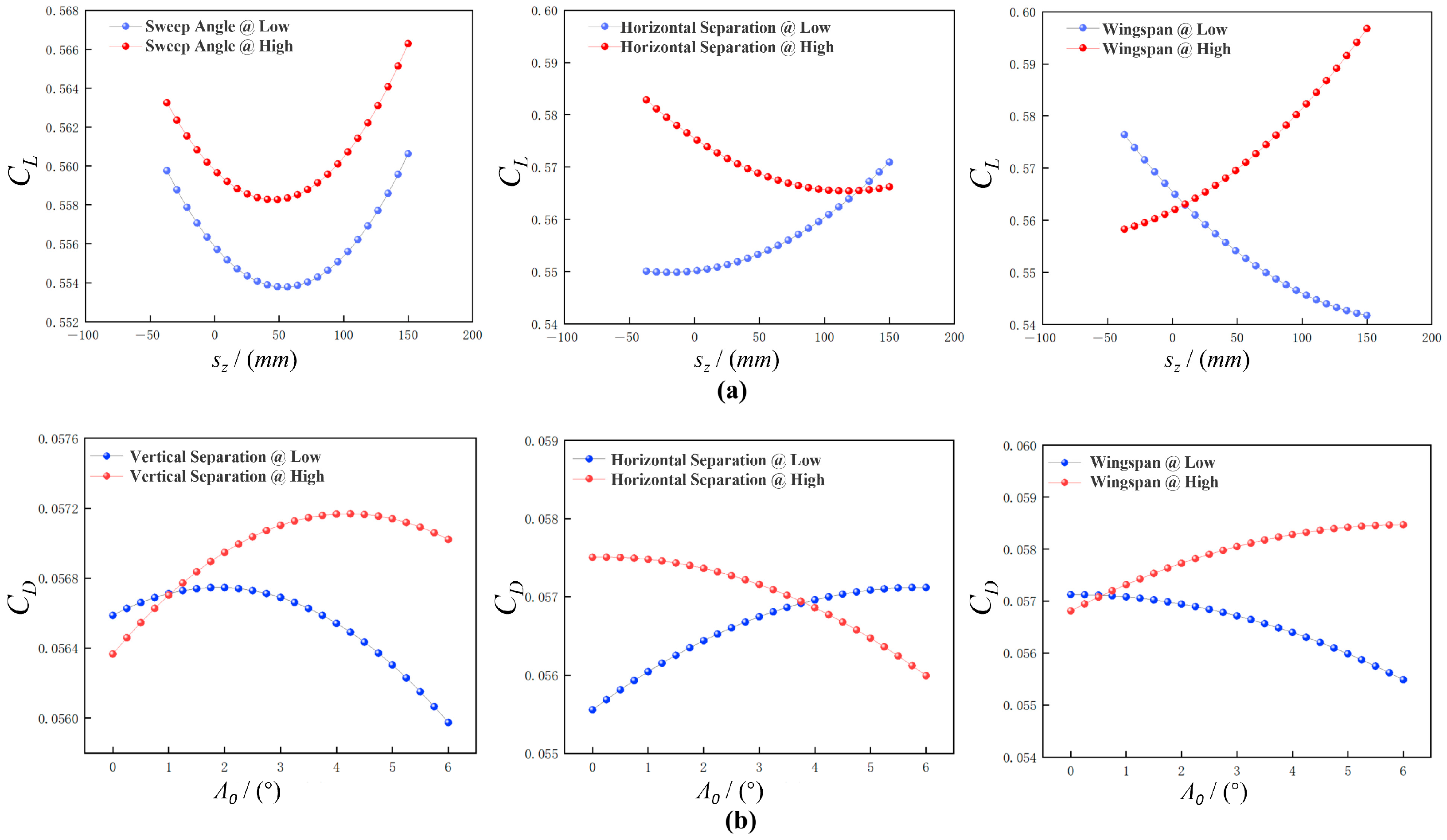
Relying solely on isolated contributions is insufficient for the tandem-wing configuration characterized by complex interference. Therefore, the analysis further incorporates interaction effects to characterize the dependency between parameters. This coupling intensity is manifested by the non-parallelism or crossing features of the response curves; a significant deviation from parallelism implies that the sensitivity of the objective function to one parameter is substantially modulated by the magnitude of another parameter, rather than being an independent superposition. Applying this principle to Figure 9, a significant crossing feature is observed in the interaction curves between the s_z and the b₁. This marked non-parallelism implies that the lift-generating efficiency of the wing span is strictly constrained by the s_z. Physically, this indicates that s_z controls the vertical location of the fore wing’s downwash wake. If s_z is not optimized in coordination with the span, the aft wing may fall directly into the wake deficit region, negating the aerodynamic benefits of a larger span.

Consequently, the analysis confirms that the four design parameters are dynamically coupled rather than independent. Despite its relatively low individual contribution, the vertical separation plays an essential synergistic role in influencing the aerodynamic lift. Therefore, all four geometric parameters are retained for the MIGA global optimization. This comprehensive variable selection ensures that the algorithm can fully exploit these parameter interaction effects, thereby facilitating the identification of the optimal configuration and maximizing the aerodynamic lift.

3.4. Optimization Results and Analysis

Prior to global optimization, the configuration yielding the maximum lift coefficient within the OLHS dataset was selected as the baseline design vector X_base, defined as:

$$x_{base}=\left[b_1,{\Lambda }_0,s_x,s_z\right]=\left[2.438 \mathrm{m},5°,0.664 \mathrm{m},0.091 \mathrm{m}\right]$$

(9)

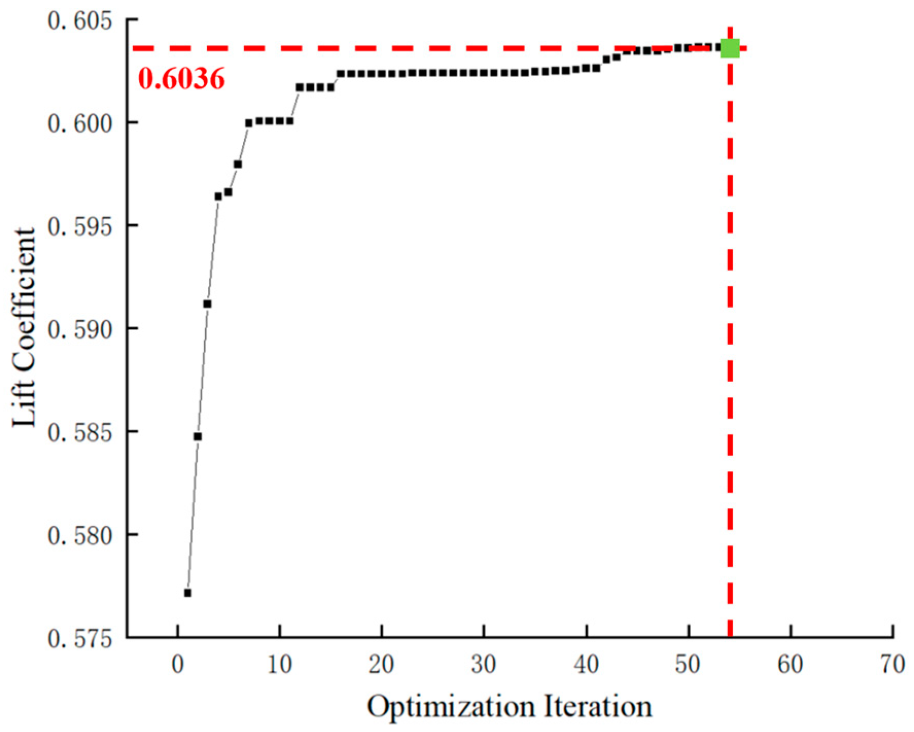
The iterative history of the lift coefficient optimization is illustrated in Figure 10. The population demonstrates a rapid performance improvement in the initial stages, driven by the elite seeding strategy. The algorithm achieves convergence approximately at the 53rd generation, stabilizing at a global optimum. The corresponding optimal design vector X_opt is identified as:

$$x_{opt}=\left[b_1,{\Lambda }_0,s_x,s_z\right]=\left[2.394 \mathrm{m},1°,0.852 \mathrm{m},0.070 \mathrm{m}\right]$$

(10)

For quantitative verification, the projected wing areas of the baseline and optimized configurations are 0.7752 m² and 0.7723 m², respectively, with a relative difference of only 0.37%. This negligible variation confirms that the observed improvement in the lift coefficient mainly arises from the improved aerodynamic efficiency under the interaction of the tandem-wing layout, rather than the change of the wing area. To ensure the consistency and comparability of aerodynamic coefficients, all coefficients (C_L, C_D, C_L/C_D, C_L^3/2/C_D) in this study are calculated based on a fixed wing reference area S_ref = 0.7752 m² corresponding to total wing area of the baseline configuration. This reference area remains constant throughout the optimization and analysis, eliminating the influence of actual wing area variation on the aerodynamic coefficients. To validate the reliability of the optimization, a high-fidelity CFD simulation is performed using the identified optimal parameters. The quantitative comparison results are summarized in

Table 6. Aerodynamic Performance Comparison between Baseline and Optimized Configurations.

Case	Method	CL	Deviation	CD	CL/CD	CL3/2/CD
Baseline	CFD Simulation	0.5841	-	0.0488	11.9693	9.1477
Optimized	Surrogate Prediction	0.6036	0.90%	-	-	-
	CFD Validation	0.6091 (+4.28%)	-	0.0465 (−4.71%)	13.0989 (+9.44%)	10.2230 (+11.76%)

Note: Values in parentheses indicate the relative change compared to the baseline configuration. Deviation = (C_L,pred − C_L,CFD)/C_L,CFD × 100%. All aerodynamic coefficients are calculated based on a fixed reference area S_ref = 0.7752 m² (baseline reference area) to eliminate the influence of actual wing area variation.

.

As indicated in Table 6, the surrogate model predicted a C_L of 0.6036, while the CFD validation yielded 0.6091. The relative deviation is merely 0.90%, demonstrating the high precision of the proposed optimization framework. Furthermore, compared to the baseline C_L of 0.5841, the optimized configuration achieves a net performance gain of 4.28%, which fully realizes the core objective of lift coefficient maximization under strict folding constraints.

In addition, the optimized configuration obtains additional improvements in range and endurance-related aerodynamic performance while achieving the core lift enhancement objective. Specifically, the lift-to-drag ratio (C_L/C_D) is the core parameter that determines the maximum flight range of fixed-wing UAVs according to the classical Breguet range equation. As shown in Table 6, C_L/C_D increases from 11.9693 of the baseline to 13.0989 of the optimized configuration, corresponding to a 9.44% improvement. This means that the optimized UAV can achieve a longer mission range under the same battery or fuel capacity, which is of high engineering value for the long-distance reconnaissance and patrol tasks of the folding UAV. Meanwhile, the parameter C_L^3/2/C_D directly governs the maximum loitering endurance of the UAV via the Breguet endurance equation. The optimized configuration achieves an 11.76% increase in this parameter, from 9.1477 to 10.2230. This substantial enhancement in endurance performance directly matches the core operational requirement of the folding tandem-wing UAV for long-time continuous loitering in the target area.

Notably, the above improvements in range and endurance performance are additional aerodynamic benefits brought by the geometric parameter adjustment for C_L maximization, with no additional drag reduction optimization design carried out in this study. This further verifies that the optimized configuration can not only meet the core lift demand under strict geometric constraints, but also obtain better comprehensive flight performance, which significantly improves the engineering application value of the proposed optimization scheme.

To further elaborate on the practical significance of the observed lift coefficient increment, the 4.28% increase in C_L directly translates to a 4.28% improvement in the maximum lift force at the same flight speed. For a small folding-wing UAV in the 10 kg takeoff weight class, this increment enables the UAV to carry an additional payload of approximately 0.43 kg under identical flight conditions. This is of critical importance for platforms with strict weight and volume constraints, as the extra payload can be used to enhance mission capabilities (e.g., adding sensors) or extend endurance by increasing fuel capacity. Meanwhile, as an additional benefit of the optimized layout, C_L/C_D improves by 9.44% and C_L^3/2/C_D by 11.76%, which contributes to extending both the cruise range and endurance of the UAV.

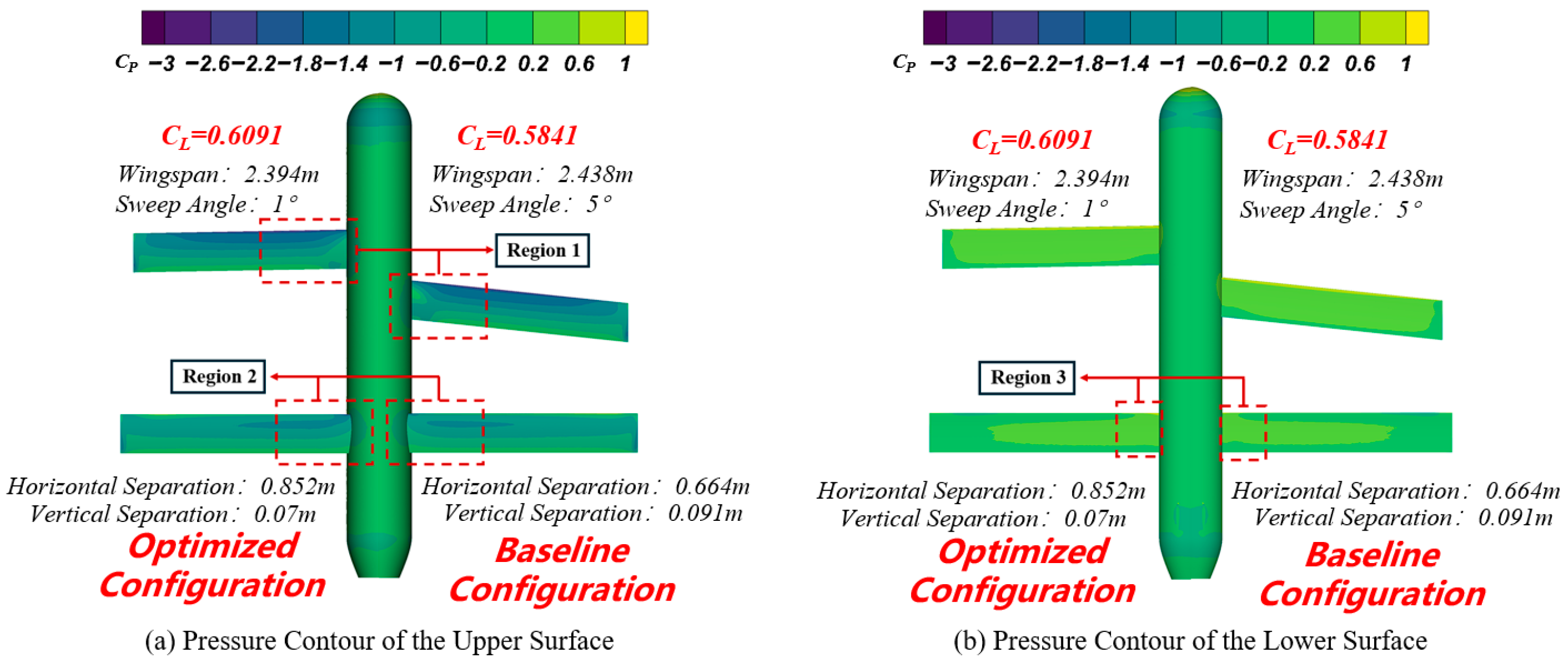
To elucidate the physical mechanism responsible for this performance gain, the surface pressure coefficient (C_P) contours of the baseline and optimized configurations are compared in Figure 11. A global inspection reveals that the pressure distribution on the fuselage remains relatively stable. The significant aerodynamic alterations are spatially concentrated at the wing root regions of both the fore and aft wings, and these variations gradually diminish along the spanwise direction towards the wingtips. Variations in the pressure distribution over partial regions reveal the changes in lift: On the upper surface (Figure 11a), particularly in Region 1 (fore wing root) and Region 2 (aft wing root), the optimized configuration exhibits a noticeable expansion and intensification of the low-pressure zones. This suggests that the flow acceleration over the upper surfaces has been effectively enhanced. Concurrently, inspection of the lower surface (Figure 11b) indicates that in Region 3 (aft wing root), the high-pressure area displays a slight increase compared to the baseline configuration. These favorable pressure topology changes are attributed to the optimized spatial arrangement. The adjustments in s_x and s_z effectively modified the aerodynamic coupling between the tandem wings. This improved interference environment specifically alleviated the suppression at the aft wing root, resulting in an enlarged low-pressure zone and, consequently, a measurable increase in the total lift coefficient.

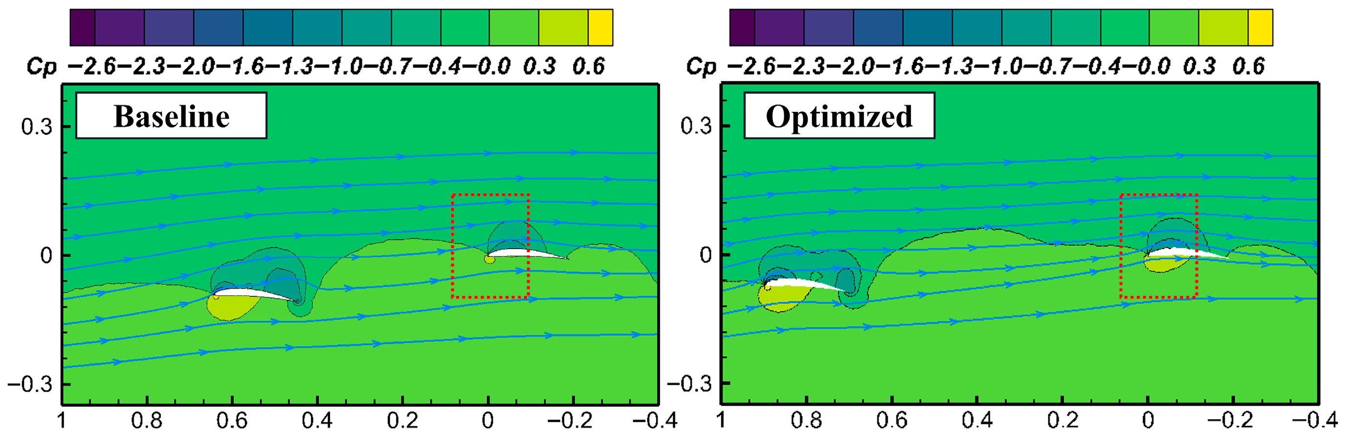
To visually elucidate the flow mechanisms driving these pressure variations, Figure 12 presents the streamlines and pressure coefficient contours at the 17% semi-span station. In the optimized configuration—characterized by increased s_x, reduced s_z, and a decreased Λ₀—the interaction between the fore wing wake and the aft wing is improved. Specifically, the modified wake effect from the fore wing induces an increase in the effective angle of attack for the aft wing. Consequently, both the high-pressure region on the lower surface and the low-pressure region on the upper surface of the aft wing are markedly expanded compared to the baseline configuration, leading to a substantial enhancement in the lift coefficient. Furthermore, the reduction in s_z helps delay flow separation on the fore wing, thereby maintaining superior aerodynamic efficiency across the tandem-wing system.

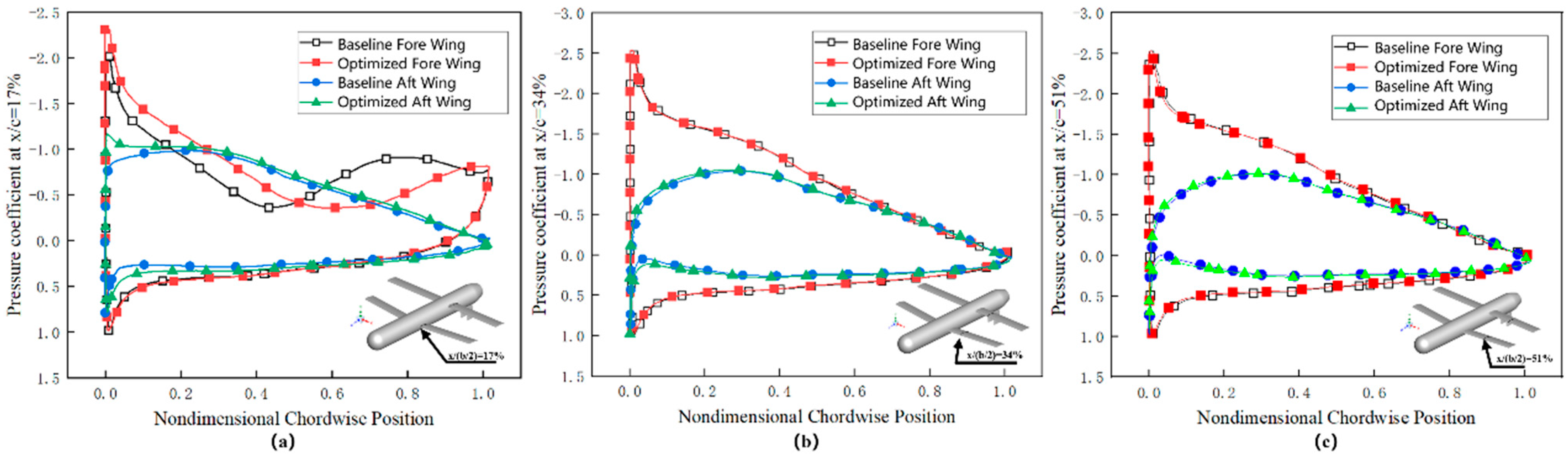
From the perspective of local analysis, pressure coefficient distributions are extracted at representative spanwise sections (17%, 34%, and 51% of the semi-span). The comparative analysis at the 17% spanwise location (Figure 13a) validates the variation of aerodynamic characteristics at the wing root, which is substantiated by the relative variation in the enclosed areas of the C_P curves. Regarding the fore wing, the optimized configuration exhibits a significantly expanded C_P envelope near the leading edge compared to the baseline, whereas in the aft chord region, it presents a faster pressure recovery gradient, indicating significant changes in the flow field characteristics at this location. Concurrently, a more distinct lift improvement is achieved on the aft wing. The optimized configuration demonstrates a comprehensive expansion of the pressure coefficient envelope across the majority of the chord length relative to the baseline. Consequently, the accumulated sectional C_L achieves a significant gain of approximately 11.4%. Conversely, the pressure distributions at the outboard sections (34% and 51%) remain nearly identical. The analysis indicates that the total lift increment of the UAV is predominantly driven by the aerodynamic improvements at the wing root region. Consequently, future optimization efforts should prioritize geometric parameters associated with the wing root to further exploit the potential for aerodynamic.

4. Conclusions

This study proposes an aerodynamic optimization method specifically for a folding tandem-wing UAV. By employing an optimization strategy that integrates a high-fidelity surrogate model with the MIGA, the search for a configuration maximizing lift under strict geometric constraints was successfully realized. The primary conclusions are summarized as follows:

(1) Global sensitivity analysis identifies the fore wing span as the dominant factor, contributing approximately 47.40% to lift performance. The fore wing sweep angle, horizontal separation, and vertical separation contribute 9.57%, 36.50%, and 6.53%, respectively. Notably, parameter analysis reveals significant interaction effects between the vertical separation—despite its lowest individual contribution—and other parameters This indicates that for low-Reynolds-number tandem wings with constrained spans, synergistically optimizing vertical separation is critical for aerodynamic enhancement.

(2) The optimization strategy, utilizing the Orthogonal Polynomial Model and MIGA with elite seeding, demonstrated high efficiency. The final configuration showed a marginal CFD prediction deviation of 0.90%, verifying the method’s reliability. Compared to the baseline, the optimized design achieved a net lift coefficient gain of 4.28%, significantly improving both payload capacity and low-speed cruising performance.

(3) The lift increment is primarily driven by flow improvements at the wing root, with minimal variation near the wing tips. The optimized configuration enhances overall lift by modulating the chordwise and spanwise pressure distributions in the root region. Consequently, the wing root remains a critical area for aerodynamic potential, and future research should focus on its geometric refinement to achieve further performance breakthroughs.

It should be noted that the current optimization focuses exclusively on the aerodynamic performance of the folding tandem-wing UAV, treating the entire airframe as a rigid body. Given the inherent structural characteristics of the folding mechanism and the complex coupling effects observed at the wing root, future research will expand into MDO. By comprehensively integrating structural stiffness and flight control stability, subsequent efforts aim to explore a broader range of conceptual design solutions with high engineering application value. Additionally, future work will also investigate the integration of modern high-performance airfoils, aiming to further enhance the aerodynamic efficiency of the tandem-wing system.

References

1. Finigian, M.; Kavounas, P.A.; Ho, I.; Smith, C.C.; Witusik, A.; Hopwood, A.; Avent, C.; Ragasa, B.; Roth, B. Design and Flight Test of a Tube-Launched Unmanned Aerial Vehicle. Aerospace 2024, 11, 133. [Google Scholar] [CrossRef]
2. Munk, M.M. The Minimum Induced Drag of Aerofoils; NACA Technical Report 121; National Advisory Committee for Aeronautics: Washington, DC, USA, 1923.
3. Prandtl, L. Applications of Modern Hydrodynamics to Aeronautics; NACA Technical Report 116; National Advisory Committee for Aeronautics: Washington, DC, USA, 1923.
4. Jones, R.; Cleaver, D.J.; Gursul, I. Aerodynamics of biplane and tandem wings at low Reynolds numbers. Exp. Fluids 2015, 56, 124. [Google Scholar] [CrossRef]
5. Zhang, Q.; Xue, R.; Li, H. Aerodynamic Exploration for Tandem Wings with Smooth or Corrugated Surfaces at Low Reynolds Number. Aerospace 2023, 10, 427. [Google Scholar] [CrossRef]
6. Scharpf, D.F.; Mueller, T.J. Experimental study of a low Reynolds number tandem airfoil configuration. J. Aircr. 1992, 29, 231–236. [Google Scholar] [CrossRef]
7. Broering, T.M.; Lian, Y. The effect of wing spacing on tandem wing aerodynamics. In Proceedings of the 28th AIAA Applied Aerodynamics Conference, Chicago, IL, USA, 28 June–1 July 2010. AIAA Paper 2010-4385. [Google Scholar] [CrossRef]
8. Cai, Y.; Liu, G.; Zhu, X.; Tu, Q.; Hong, G. Aerodynamic interference significance analysis of two-dimensional front wing and rear wing airfoils with stagger and gap variations. J. Aerosp. Eng. 2019, 32, 04019098. [Google Scholar] [CrossRef]
9. Delikan, M.; Bal, Ş. A comprehensive CFD analysis of tandem foils with and without ground effect. J. Nav. Archit. Mar. Technol. 2025, 227, 1–21. [Google Scholar] [CrossRef]
10. Shah, S.H.R.; Ahmed, A. On the secondary stall of a wing in tandem configuration. Aeronaut. J. 2024, 128, 1729–1742. [Google Scholar] [CrossRef]
11. Cheng, H.; Wang, H. Prediction of lift coefficient for tandem wing configuration or multiple-lifting-surface system using Prandtl’s lifting-line theory. Int. J. Aerosp. Eng. 2018, 2018, 3104902. [Google Scholar] [CrossRef]
12. Figat, M.; Kwiek, A. Analysis of longitudinal dynamic stability of tandem wing aircraft. Aircr. Eng. Aerosp. Technol. 2023, 95, 1411–1422. [Google Scholar] [CrossRef]
13. Goetzendorf-Grabowski, T. Flight dynamics of unconventional configurations. Prog. Aerosp. Sci. 2023, 137, 100885. [Google Scholar] [CrossRef]
14. Cheng, H.; Wang, H.; Shi, Q.; Zhang, M. Unsteady aerodynamics investigation of deploying tandem-wing with different methods. Proc. Inst. Mech. Eng. Part G J. Aerosp. Eng. 2019, 233, 3714–3733. [Google Scholar] [CrossRef]
15. Kostić, I.; Simonović, A.; Kostić, O.; Ivković, D.; Tanović, D. Lateral-directional aerodynamic optimization of a tandem wing UAV using CFD analyses. Aerospace 2024, 11, 223. [Google Scholar] [CrossRef]
16. Shi, Y.; Lan, X.; Wang, Y.; Yang, T.; Liu, Y. Data mining-based design space exploration and optimization for tandem airfoils. Int. J. Aerosp. Eng. 2023, 2023, 3513507. [Google Scholar] [CrossRef]
17. Queipo, N.V.; Haftka, R.T.; Shyy, W.; Goel, T.; Vaidyanathan, R.; Tucker, P.K. Surrogate-based analysis and optimization. Prog. Aerosp. Sci. 2005, 41, 1–28. [Google Scholar] [CrossRef]
18. Simpson, T.W.; Poplinski, J.D.; Koch, P.N.; Allen, J.K. Metamodels for computer-based engineering design: Survey and recommendations. Eng. Comput. 2001, 17, 129–150. [Google Scholar] [CrossRef]
19. Forrester, A.I.J.; Sóbester, A.; Keane, A.J. Engineering Design via Surrogate Modelling: A Practical Guide; Wiley: Chichester, UK, 2008. [Google Scholar] [CrossRef]
20. Han, Z.-H.; Görtz, S.; Zimmermann, R. Improving variable-fidelity surrogate modeling via gradient-enhanced kriging and a generalized hybrid bridge function. Aerosp. Sci. Technol. 2013, 25, 177–189. [Google Scholar] [CrossRef]
21. Krishnamurthy, T. Response surface approximation with augmented and compactly supported radial basis functions. In Proceedings of the 44th AIAA/ASME/ASCE/AHS/ASC Structures, Structural Dynamics, and Materials Conference, Norfolk, VA, USA, 7–10 April 2003. AIAA Paper 2003-1748. [Google Scholar] [CrossRef]
22. Giunta, A.A.; Watson, L.T. A comparison of approximation modeling techniques: Polynomial versus interpolating models. In Proceedings of the 7th AIAA/USAF/NASA/ISSMO Symposium on Multidisciplinary Analysis and Optimization, St. Louis, MO, USA, 2–4 September 1998. AIAA Paper 98-4758. [Google Scholar] [CrossRef]
23. McKay, M.D.; Beckman, R.J.; Conover, W.J. A comparison of three methods for selecting values of input variables in the analysis of output from a computer code. Technometrics 1979, 21, 239–245. [Google Scholar] [CrossRef] [PubMed]
24. Holland, J.H. Adaptation in Natural and Artificial Systems: An Introductory Analysis with Applications to Biology, Control, and Artificial Intelligence; The MIT Press: Cambridge, MA, USA, 1992. [Google Scholar] [CrossRef]
25. Gong, C.L.; Gu, L.X. Genetic algorithm based global optimization algorithm used to solving system analysis of multi-disciplinary optimization. In Proceedings of the 2010 IEEE International Conference on Intelligent Computing and Intelligent Systems (ICICIS), Xiamen, China, 29–31 October 2010; pp. 325–329. [Google Scholar] [CrossRef]
26. Yan, X.; Zhu, J.; Kuang, M.; Wang, X. Aerodynamic shape optimization using a novel optimizer based on machine learning techniques. Aerosp. Sci. Technol. 2019, 86, 826–835. [Google Scholar] [CrossRef]
27. Zhang, B.; Feng, Z.; Xu, B.; Yang, T. Efficient aerodynamic shape optimization of the hypersonic lifting body based on free form deformation technique. IEEE Access 2019, 7, 147991–148003. [Google Scholar] [CrossRef]
28. Liang, Y.; Cheng, X.; Li, Z.; Xiang, J. Robust multi-objective wing design optimization via CFD approximation model. Eng. Appl. Comput. Fluid Mech. 2011, 5, 286–300. [Google Scholar] [CrossRef]
29. Du, Y.M.; Li, Z.H.; Wang, H.; Huang, L.T.; Gao, P. Shape and parameter optimizations on a high-lift configuration with flap-based circulation control. Phys. Fluids 2025, 37, 087113. [Google Scholar] [CrossRef]
30. Gong, C.; Ma, B.-F. Shape optimization and sensitivity analysis of a morphing-wing aircraft. Int. J. Aeronaut. Space Sci. 2019, 20, 57–69. [Google Scholar] [CrossRef]
31. Qian, Z.; Seepersad, C.C.; Joseph, V.R.; Allen, J.K.; Wu, C.F.J. Building surrogate models based on detailed and approximate simulations. J. Mech. Des. 2006, 128, 668–677. [Google Scholar] [CrossRef]
32. Karatzas, E.; Nikolaou, E.; Pitsis, A.; Alexopoulos, S.; Roussos, S.; Georgantakis, E.; Lappas, V.; Kostopoulos, V. Conceptual design and analysis of a tube-launched fixed-wing UAV with integrated folding wing systems. Aerosp. Sci. Technol. 2026, 168, 111248. [Google Scholar] [CrossRef]
33. Karatzas, E.; Nikolaou, E.; Pitsis, A.; Alexopoulos, S.; Lappas, V.; Kostopoulos, V. Wing Design for Class I Mini Unmanned Aerial Vehicles—Special Considerations for Foldable Wing Configuration at Low Reynolds Numbers. Eng. Proc. 2025, 90, 96. [Google Scholar] [CrossRef]
34. Selig, M.S.; Guglielmo, J.J. High-lift low Reynolds number airfoil design. J. Aircr. 1997, 34, 72–79. [Google Scholar] [CrossRef]
35. Wang, X.; Lu, W.; Liu, W.; Chen, C.; Zhao, L. Aerodynamic analysis of a logistics UAV with foldable bi-wing configuration. Int. J. Aerosp. Eng. 2023, 2023, 3304048. [Google Scholar] [CrossRef]
36. Reynolds, O. On the dynamical theory of incompressible viscous fluids and the determination of the criterion. Philos. Trans. R. Soc. A 1895, 186, 123–164. [Google Scholar] [CrossRef]
37. Menter, F.R. Two-equation eddy-viscosity turbulence models for engineering applications. AIAA J. 1994, 32, 1598–1605. [Google Scholar] [CrossRef]
38. Wang, X.; Liu, W.; Chen, C.; Liu, Y. Rotor position aerodynamics research of a hybrid configuration electric UAV. Aircr. Eng. Aerosp. Technol. 2025, 97, 739–749. [Google Scholar] [CrossRef]
39. Shah, S.H.R. Aerodynamics of Wings in Tandem at Low Reynolds Numbers. Ph.D. Dissertation, Auburn University, Auburn, AL, USA, 2023. [Google Scholar]
40. Giunta, A.A.; Wojtkiewicz, S.F.; Eldred, M.S. Overview of modern design of experiments methods for computational simulations. In Proceedings of the 41st Aerospace Sciences Meeting and Exhibit, Reno, NV, USA, 6–9 January 2003. AIAA Paper 2003-649. [Google Scholar] [CrossRef]
41. Jin, R.; Chen, W.; Sudjianto, A. An efficient algorithm for constructing optimal design of computer experiments. J. Stat. Plan. Inference 2005, 134, 268–287. [Google Scholar] [CrossRef]
42. Morris, M.D.; Mitchell, T.J. Exploratory designs for computational experiments. J. Stat. Plan. Inference 1995, 43, 381–402. [Google Scholar] [CrossRef]
43. Sayal, A.; Jha, J.; Chaithra, N.; Nithin, A.; Shankar, B.; Gupta, A. Orthogonal polynomials and their engineering applications. In Business Data Analytics; Singh, R., Gehlot, A., Eds.; Communications in Computer and Information Science; Springer: Cham, Switzerland, 2025; pp. 169–186. [Google Scholar] [CrossRef]
44. Krige, D.G. A statistical approach to some basic mine valuation problems on the Witwatersrand. J. S. Afr. Inst. Min. Metall. 1951, 52, 119–139. [Google Scholar]
45. Cressie, N. Spatial prediction and ordinary kriging. Math. Geol. 1988, 20, 405–421. [Google Scholar] [CrossRef]
46. Mullur, A.A.; Messac, A. Extended radial basis functions: More flexible and effective metamodeling. AIAA J. 2005, 43, 1306–1315. [Google Scholar] [CrossRef]
Figure 1. Technical Route and Research Methodology.
Aerospace 13 00224 g001
Figure 2. Aerodynamic Configuration of the UAV.
Aerospace 13 00224 g002
Figure 3. Flow Field Grid of the UAV.
Aerospace 13 00224 g003
Figure 4. Grid Details of the Validation Model.
Aerospace 13 00224 g004
Figure 5. Validation of CFD Method. (a) Fore wing validation; (b) Aft wing validation.
Aerospace 13 00224 g005
Figure 6. Comparison of Sampling Characteristics. (a) Latin Hypercube Sampling; (b) Optimal Latin Hypercube Sampling.
Aerospace 13 00224 g006
Figure 7. Comparison between Actual and Predicted Lift-Drag Characteristics. (a) Comparison between Actual and Predicted Values of Lift Coefficient; (b) Comparison between Actual and Predicted Values of Drag Coefficient.
Aerospace 13 00224 g007
Figure 8. Pareto Contribution of Parameters to Aerodynamic Characteristics.
Aerospace 13 00224 g008
Figure 9. Analysis of Parameter Interaction Effects. (a) Interaction Effects between sz and Other Parameters for CL; (b) Interaction Effects between Λ0 and Other Parameters for CD.
Aerospace 13 00224 g009
Figure 10. Iterative Process for CL.
Aerospace 13 00224 g010
Figure 11. Comparison of Pressure Coefficient Distributions. (a) Pressure Contour of the Upper Surface; (b) Pressure Contour of the Lower Surface.
Aerospace 13 00224 g011
Figure 12. Pressure Coefficient Contours and Velocity Streamlines at the 17% Semi-span Section.
Aerospace 13 00224 g012
Figure 13. Comparison of Pressure Coefficients on Representative Sections. (a) CP Comparison for the Cross Section at 17% Spanwise Position; (b) CP Comparison for the Cross Section at 34% Spanwise Position; (c) CP Comparison for the Cross Section at 51% Spanwise Position.
Aerospace 13 00224 g013