Effects of Expansion Corner on Linear and Non-Linear Three-Dimensional Boundary Layer Stability

Abstract

The transition of hypersonic boundary layers remains a significant unresolved challenge in fluid mechanics, particularly regarding the influence of expansion corners on three-dimensional boundary layer instability. The present work investigates a hypersonic swept wing configuration with an expansion corner using linear stability theory (LST) and direct numerical simulations (DNSs). A high-order shock-fitting method provides the laminar base flow for sweep angles of ${30}^{\circ }$, ${45}^{\circ }$ and ${60}^{\circ }$ and expansion corner angles of $0^{\circ }$, $3^{\circ }$ and $6^{\circ }$. As the sweep and expansion angles increase, both the favourable pressure gradient and crossflow intensity are strengthened. LST reveals that, while the expansion corner suppresses disturbance growth locally, it promotes the development of subharmonic modes downstream, with the dominant spanwise wavelength doubling across the corner. Crossflow instability intensifies with increasing sweep and expansion angles. DNSs accounting for non-parallel effects confirm a sharp reduction in growth rate at the corner itself, while upstream and downstream trends remain consistent with LST predictions. Nonlinear simulations with finite-amplitude perturbations show saturated crossflow vortex structures. The subharmonic mode develops into mushroom-shaped vortices distinct from those in conventional studies. The expansion corner weakens the vortex intensity for both spanwise wavelengths, exerting a complex effect on the transition process.

1. Introduction

For more than a century, the problems of flow stability and transition have captivated applied mathematicians and fluid dynamicists. Beyond the inherent theoretical and experimental challenges, a primary drive for research into boundary layer stability is the need to understand, predict, and control the transition to turbulence. The origin of turbulence and the transition from laminar to turbulent flow remain among the most significant unsolved problems in fluid mechanics and aerodynamics [1,2]. This challenge is particularly acute in the context of hypersonic vehicles, where boundary layer instability and transition are critical phenomena affecting skin friction drag, aerodynamic heating, and ultimately the success of a flight mission. Consequently, the instability and transition of high-speed flows are regarded as fundamental scientific issues in the design of hypersonic vehicles.

In low-disturbance environments typical of hypersonic flight, transition often follows the classical route involving the linear growth of instability waves, their nonlinear interactions, and eventual breakdown to turbulence [3]. For high-speed vehicles, understanding the linear and nonlinear mechanisms governing the evolution of these instabilities is paramount. While transition models [4,5] offer practical tools for engineering design, a deeper mechanistic understanding relies heavily on stability theory. This is especially true for three-dimensional boundary layers, where the crossflow instability often dominates the transition process on swept wings and other relevant configurations [1,6].

The crossflow instability arises in three-dimensional boundary layers due to the imbalance between the pressure gradient perpendicular to the inviscid streamline and centrifugal forces, leading to a secondary flow within the boundary layer [7]. The crossflow velocity profile has inherently an inflection point, making it susceptible to inviscid instability mechanisms [8]. This instability manifests as co-rotating vortices aligned approximately with the inviscid flow direction. Crossflow modes are typically categorized into stationary waves (zero frequency), often excited by surface roughness, and travelling waves (non-zero frequency), by freestream turbulence noise. Although linear stability theory (LST) often predicts higher growth rates for travelling waves, transition in low-turbulence flight conditions is frequently initiated by the subcritical growth of stationary modes [9]. The nonlinear evolution of these stationary crossflow vortices modifies the base flow, creating strong shear layers that are susceptible to high-frequency secondary instabilities, which ultimately lead to breakdown [7,10,11]. This saturation and secondary instability process have been extensively studied in low-speed flows using tools such as nonlinear parabolized stability equations (NPSE), secondary instability theory (SIT), and direct numerical simulation (DNS) [12,13,14].

In the hypersonic regime, the compressibility introduces additional complexity. For three-dimensional hypersonic boundary layers, both crossflow and Mack-type instabilities can coexist and potentially interact [15,16,17]. Recent flight experiments (e.g., HIFiRE, BOLT) and ground-test studies have provided valuable data, but measuring the small-scale crossflow structures within the boundary layer remains challenging [18,19]. Numerical studies have successfully applied LST, PSE, and DNS to hypersonic crossflow problems. While in some cases modulated by high-enthalpy and thermal-chemical non-equilibrium effects, the fundamental saturation and secondary instability mechanisms are revealed to share key similarities with their incompressible counterparts [20,21].

Despite these advances, most fundamental studies on crossflow instability have focused on idealized geometries like disks, swept cylinders, swept wings, primarily in the incompressible or transonic regime. The understanding of crossflow instability on practical hypersonic vehicle geometries, which often feature complex surface contours, is still limited. In particular, expansion corners, which are common features at the wings of hypersonic vehicles, can significantly alter the development of the boundary layer instability modes. Although the influence of compression corners on flow stability has been investigated to some extent, the effect of expansion corners is relatively unexplored [22], particularly within the context of three-dimensional hypersonic boundary layers. Early studies suggested that expansion corners can re-laminarize turbulent flow by accelerating the flow and weakening turbulent structures [23]. In contrast to incompressible case, recent experiments and LST analyses for two-dimensional supersonic flows indicate that expansion corners can have a strong stabilizing effect on the second mode [24,25]. However, their effect on the linear and nonlinear development of three-dimensional crossflow instabilities in hypersonic flows is essentially unknown.

This study is therefore motivated to systematically investigate the effects of an expansion corner on the stability of a three-dimensional hypersonic boundary layer, focusing on the linear and nonlinear evolution of crossflow vortices. We establish a representative swept wing configuration with an expansion corner and compute laminar base flows using high-accuracy numerical methods, examining the influence of sweep and expansion angles through a parametric study. Linear stability analysis is employed to identify stationary crossflow modes, quantify the impact of the expansion corner on their growth, and elucidate the underlying physical mechanisms via energy budget analysis, with results validated against DNS to account for non-parallel effects. Finally, DNS is used to investigate the nonlinear evolution of the most unstable modes, focusing on how the expansion corner affects the saturation process and the emergence of secondary instabilities across different spanwise wavelengths.

The remainder of this paper is organized as follows. Section 2 describes the geometrical models, the numerical methods for base flow computation, and the theoretical frameworks for linear stability analysis and DNS. Section 3 outlines the key characteristics of the base flow. The linear and nonlinear evolution of the stationary crossflow modes are presented in Section 4 and Section 5, respectively. Finally, Section 6 summarizes the key findings and discusses their implications.

2. Mathematical Formulation

2.1. Problem Statement

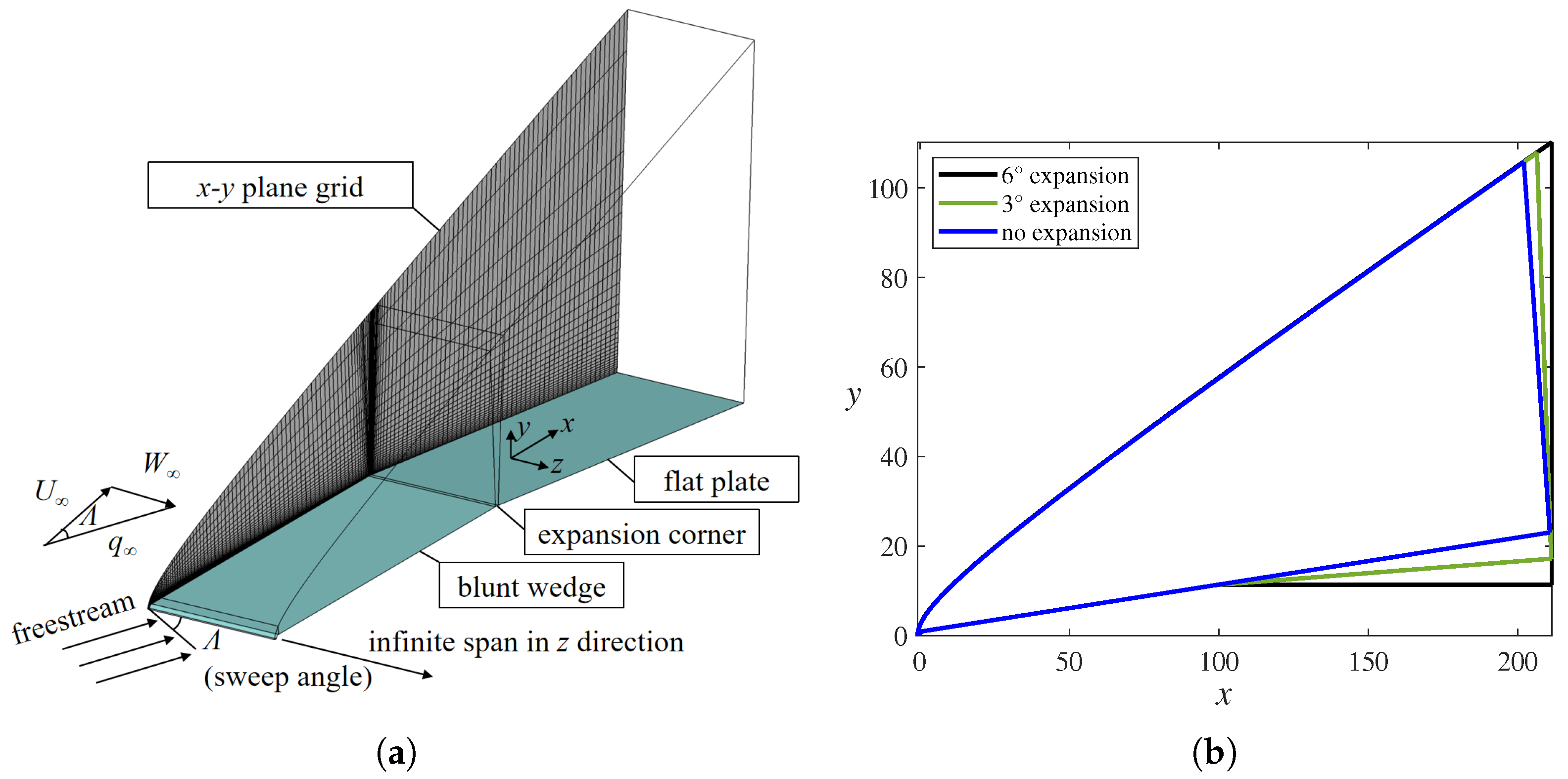
To simulate the boundary layer flow over an infinite swept wing, the computational model employed in this study is illustrated in Figure 1a. The model features a blunt-nosed wedge connecting to a flat plate, forming an expansion corner that is the focus of this research. The relevant characteristic scales of the model include the leading-edge radius $R^{*}$, the half-wedge angle $\theta$, the streamwise domain size $L_s^{*}$, and the curvature radius at the expansion corner $R_e^{*}$. Unless stated otherwise, all lengths are non-dimensionalized by $R^{*}$.

For the computation of the unperturbed laminar base flow, the assumption of spanwise invariance (infinite swept wing) allows the problem to be solved in a two-dimensional plane. Consequently, the spanwise length ${\lambda }_z^{*}$ is irrelevant for this step. However, all three velocity components are computed, hence this base flow calculation is often referred to as a quasi-two-dimensional computation. In the present setup, the z-axis is aligned with the leading-edge stagnation line, the x-axis is perpendicular to the leading edge within the wing plane, and the y-axis is normal to the $x-z$ surface. Since the computational x-y plane is defined perpendicular to the leading edge, the freestream velocity must be decomposed within this plane as $U_{\infty }=q_{\infty }cos\Lambda$ and $W_{\infty }=q_{\infty }sin\Lambda$, where $q_{\infty }$ is the total freestream velocity magnitude, $U_{\infty }$ is its component in the x-direction, $W_{\infty }$ is its spanwise component, and $\Lambda$ is the sweep angle of the leading edge. All cases considered in this study have zero angle of attack; thus, the freestream velocity has no component in the y-direction.

When introducing flow disturbances for stability analysis, the assumption of spanwise invariance is no longer valid, and full three-dimensional computations are necessary. In these simulations, the spanwise domain length, $L_z^{*}$, is determined by the spanwise wavelength of the introduced perturbations, and is set to accommodate exactly two spanwise wavelengths in the present study. The final parameters defining the model are summarized in

Table 1. Parameters of the swept wing model in the current study.

${\mathit{R}}^{*}\left(\mathbf{mm}\right)$	$\mathit{\theta } {(}^{\circ })$	${\mathit{L}}_{\mathit{s}}^{*}\left(\mathbf{mm}\right)$	${\mathit{R}}_{\mathit{e}}^{*}\left(\mathbf{mm}\right)$
2	6	424.92	22.7

.

The working conditions are selected to simulate the realistic inflow conditions of a hypersonic vehicle at a flight altitude of 27 km, as shown in

Table 2. Working conditions.

Freestream Mach Number $\mathbf{Ma}$	Freestream Reynolds Number ${\mathit{\Re }}_{\mathit{\infty }}(/\mathbf{m})$	Freestream Static Temperature ${\mathit{T}}_{\mathit{\infty }}^{*}$(K)	Prandtl Number Pr	Specific Heat Ratio $\mathit{\gamma }$
6	$3.521\times {10}^6$	224	0.72	1.4

. The relevant parameters are listed in the table below. Additionally, the freestream density is $0.0293\mathrm{kg}/{\mathrm{m}}^3$ and the static pressure is $1880\mathrm{Pa}$. The sweep angles studied are ${30}^{\circ }$, ${45}^{\circ }$, and ${60}^{\circ }$, with particular emphasis on the stability characteristics at ${60}^{\circ }$ sweep. To isolate the effect of the expansion corner magnitude, comparative cases with expansion angles of $0^{\circ }$ (i.e., no expansion effect) and $3^{\circ }$ are also investigated to examine the influence of a progressively increasing expansion angle on crossflow stability. A schematic of the computational domains for different expansion angles is shown in Figure 1b. The streamwise extent is consistent across the three different cases, and the sweep angle is fixed at ${60}^{\circ }$, resulting in nearly identical shock wave positions.

2.2. Governing Equations

2.2.1. Base Flow Calculation

Hypersonic stability analysis requires high-quality laminar base flow calculation. To obtain a smooth and accurate fundamental flow field, this paper employs a high-order accurate shock-fitting finite difference method for the calculation of the three-dimensional boundary layer base flow. Since this method uses moving shocks as the far-field boundary, the program adopts a dynamic grid method, and there exists the following transform relationship between the physical coordinates and the computational coordinates:

$$\left\{\begin{array}{c}\xi =\xi \left(x,y,t\right)\\ \eta =\eta \left(x,y,t\right)\\ \zeta =z\\ \tau =t\end{array}\right., J=\left|\begin{array}{cccc}{x}_{\xi }& x_{\eta }& 0& x_{\tau }\\ y_{\xi }& y_{\eta }& 0& y_{\tau }\\ 0& 0& 1& 0\\ 0& 0& 0& 1\end{array}\right|.$$

(1)

The control equations are the compressible Navier–Stokes equations, which can be expressed as follows:

$${\displaystyle \frac{1}{J}}{\displaystyle \frac{\partial U}{\partial \tau }}+{\displaystyle \frac{\partial F_{inv}}{\partial \xi }}+{\displaystyle \frac{\partial G_{inv}}{\partial \eta }}+{\displaystyle \frac{\partial H_{inv}}{\partial \zeta }}+U{\displaystyle \frac{\partial }{\partial \tau }}\left({\displaystyle \frac{1}{J}}\right)={\displaystyle \frac{1}{\mathrm{Re}}}\left[{\displaystyle \frac{\partial F_{vis}}{\partial \xi }}+{\displaystyle \frac{\partial G_{vis}}{\partial \eta }}+{\displaystyle \frac{\partial H_{vis}}{\partial \zeta }}\right],$$

(2)

where $U={[\rho ,\rho u,\rho v,\rho w,\rho E]}^{\top }$. The flow quantities are non-dimensionalized using the freestream values except that the reference pressure is $\gamma M{a}^2{p}_{\infty }$.

The wall is treated as adiabatic. Owing to the zero angle of attack, a symmetry condition is imposed along the centerline. The Rankine-Hugoniot relation is satisfied at the shock boundary, and a characteristic-based outflow condition is applied at the downstream boundary.

The working fluid is air, satisfying the assumptions of the calorically perfect gas. Under the present freestream conditions, the maximum temperature within the boundary layer remains well below 2000 K, ensuring that real gas effects such as vibrational excitation and dissociation are negligible, thereby justifying the calorically perfect gas assumption. The viscosity is calculated by Sutherland’s law.The base flow is calculated using in-house shock-fitting DNS code [26]. The fifth-order upwind scheme (for inviscid flux) together with the sixth-order centre scheme (for viscous flux) is used to compute the flow field [27]. A fourth-order Runge–Kutta method is applied for the time integration.

2.2.2. Stability Analysis

The stability theory investigates the spatio-temporal evolution of small disturbances introduced into a laminar base flow. The total flow field is decomposed into a steady base flow $q_B$ and a disturbance q:

$$q_{total}=q_B+q,$$

(3)

where $q={\left(\rho ,u,v,w,T\right)}^{\top }$ denotes the vector of perturbation quantities. Substituting this decomposition into the compressible Navier–Stokes equations and subtracting the equations satisfied by the base flow yields the governing equations for the perturbations:

$$\begin{array}{cc}\hfill \Gamma {\displaystyle \frac{\partial q}{\partial t}}+A{\displaystyle \frac{\partial q}{\partial x}}+B{\displaystyle \frac{\partial q}{\partial y}}+C{\displaystyle \frac{\partial q}{\partial z}}+Dq=& H_{xx}{\displaystyle \frac{{\partial }^{2}q}{\partial x^2}}+H_{yy}{\displaystyle \frac{{\partial }^{2}q}{\partial y^2}}+H_{zz}{\displaystyle \frac{{\partial }^{2}q}{\partial z^2}}+\hfill \\ \hfill & H_{xy}{\displaystyle \frac{{\partial }^{2}q}{\partial x\partial y}}+H_{yz}{\displaystyle \frac{{\partial }^{2}q}{\partial y\partial z}}+H_{xz}{\displaystyle \frac{{\partial }^{2}q}{\partial x\partial z}}+N,\hfill \end{array}$$

(4)

where the coefficient matrix can be found in Ref. [28], and the nonlinear term N is neglected in this study. For local analysis, the perturbation can be written in a wave-like form as:

$$q(x,y,z,t)=\widehat{q}\left(y\right)exp\left[i\theta (x,z,t)\right]+c.c.,$$

(5)

where $\widehat{q}$ is the shape function, c.c. denotes the complex conjugate, and the phase function $\theta$ is:

$$\theta (x,z,t)=\alpha x+\beta z-\omega t.$$

(6)

Here, $\alpha$ and $\beta$ are the wavenumbers along streamwise and spanwise directions, $\omega$ represents the angular frequency. For a spatial stability analysis, $\beta$ and $\omega$ are assumed to be real, whereas $\alpha$ is complex, $\alpha ={\alpha }_r+i{\alpha }_i$. Its real part ${\alpha }_r$ corresponds to the physical streamwise wavenumber, and its negative imaginary part $-{\alpha }_i$ gives the spatial growth rate of the perturbation. Since crossflow instability is typically dominated by stationary crossflow modes, the present study focuses primarily on the stability characteristics of the modes corresponding to $\omega =0$. Substituting Equation (5) into Equation (4), the perturbation equations reduce to a generalized eigenvalue problem as:

$$L\widehat{q}=\alpha R\widehat{q},$$

(7)

where L and R represents linear operators. Together with the boundary conditions of vanishing perturbations at the wall and in the freestream, the generalized eigenvalue problem is solved using the in-house code as in Ref. [26].

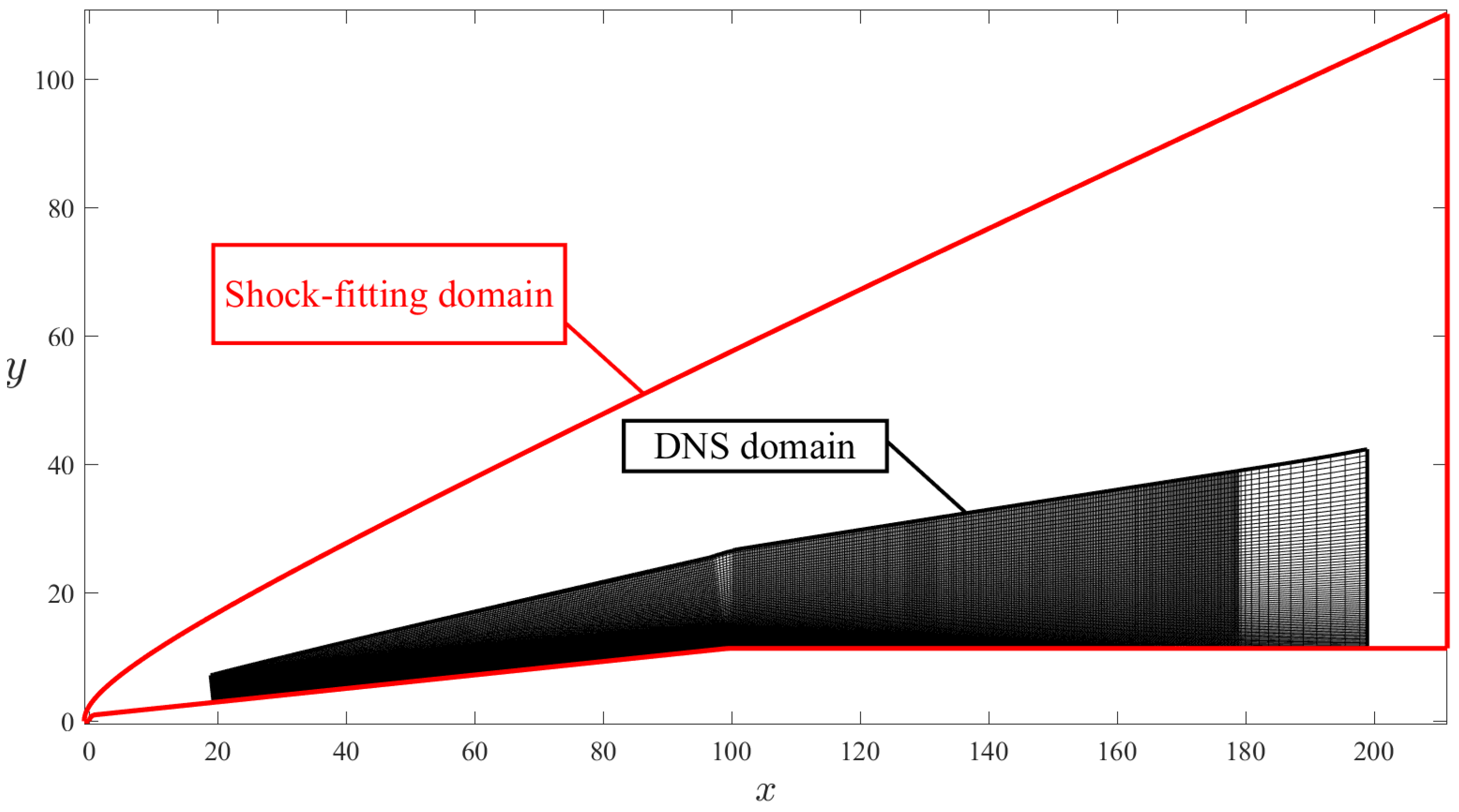
To accurately simulate the linear and nonlinear development of instability modes, three-dimensional high-fidelity direct numerical simulations (DNS) are performed in the near-wall region. The two-dimensional x-y planar slice of the computational domain is shown in Figure 2. At the inlet boundary ($s=20$, where s denotes the streamwise coordinate), disturbance profiles predicted by linear stability theory (LST) are imposed. The simulations are conducted using the well-validated CFD solver OpenCFD [29]. Spatial discretisation of the inviscid fluxes is performed with a seventh-order weighted essentially non-oscillatory (WENO) scheme in characteristic variables, while the viscous terms are discretised using a standard eighth-order central difference scheme. Time integration is carried out via an explicit third-order total variation diminishing Runge–Kutta method.

2.2.3. Simulation Strategy

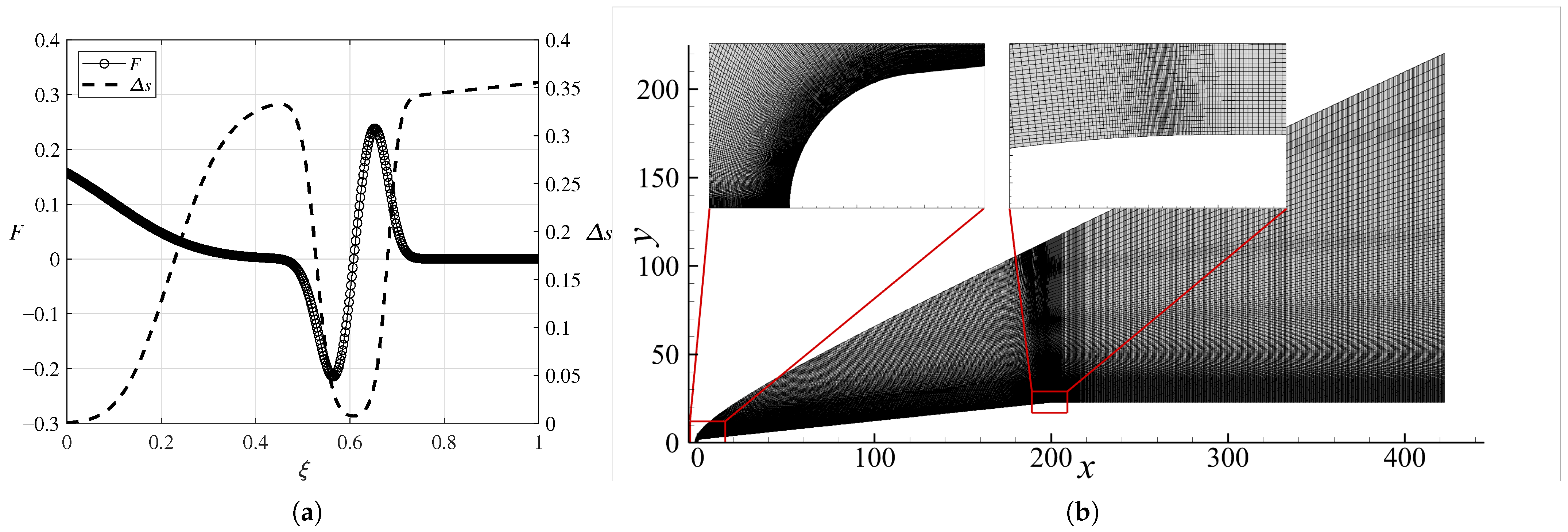
The computational grid for base flow calculation is a curvilinear body-fitted structured code-generated grid. The meshing strategy ensures a smooth transition in the distribution of grid spacing in the flow direction, and the spacing is densified near the leading edge and the expansion corner. The streamwise grid spacing is determined by

$$\begin{array}{c}F={\displaystyle \sum _{i=1}^4}{a}_i\mathrm{erf}\left[{\sigma }_i\left(\xi -b_i\right)+{(-1)}^{e_i}\right],\\ x_s=x_s\left(\xi \right),{\displaystyle \frac{d^2{x}_s}{d{\xi }^2}}={\displaystyle \frac{F}{2{\Delta }_{\xi }}}{\displaystyle \frac{d{x}_s}{d\xi }}, \\ x_s\left(0\right)=0, x_s\left(1\right)=1, \xi \in \left[0,1\right],\end{array}$$

(8)

where F is the grid-stretching function, $a_i$, $b_i$, ${\sigma }_i$, $e_i$ are the coefficients listed below in

Table 3. Parameters for the streamwise grid stretching of the swept wing model.

Index i	${\mathit{a}}_{\mathit{i}}$	${\mathit{\sigma }}_{\mathit{i}}$	${\mathit{b}}_{\mathit{i}}$	${\mathit{e}}_{\mathit{i}}$
1	−0.105	5	0.095	1
2	−0.27	20	0.552	2
3	0.45	20	0.502	2
4	−0.1797	30	0.677	2

, ${\Delta }_{\xi }$ is the grid spacing of $\xi$ coordinate, and the actual streamwise coordinate $s=x_s·L_s$, where s denotes the wall arc-length coordinate ranging from 0 (leading-edge) to $L_s$ (end of the swept wing).

In the wall-normal direction, grids cluster near the wall surface in the following manner:

$$y=a{\displaystyle \frac{1+\eta }{b-\eta }}, a={\displaystyle \frac{y_i{y}_{max}}{y_{max}-2y_i}}, b=1+{\displaystyle \frac{2a}{y_{max}}}, \eta \in \left[-1,1\right],$$

(9)

where $y_i=0.3y_{max}$.

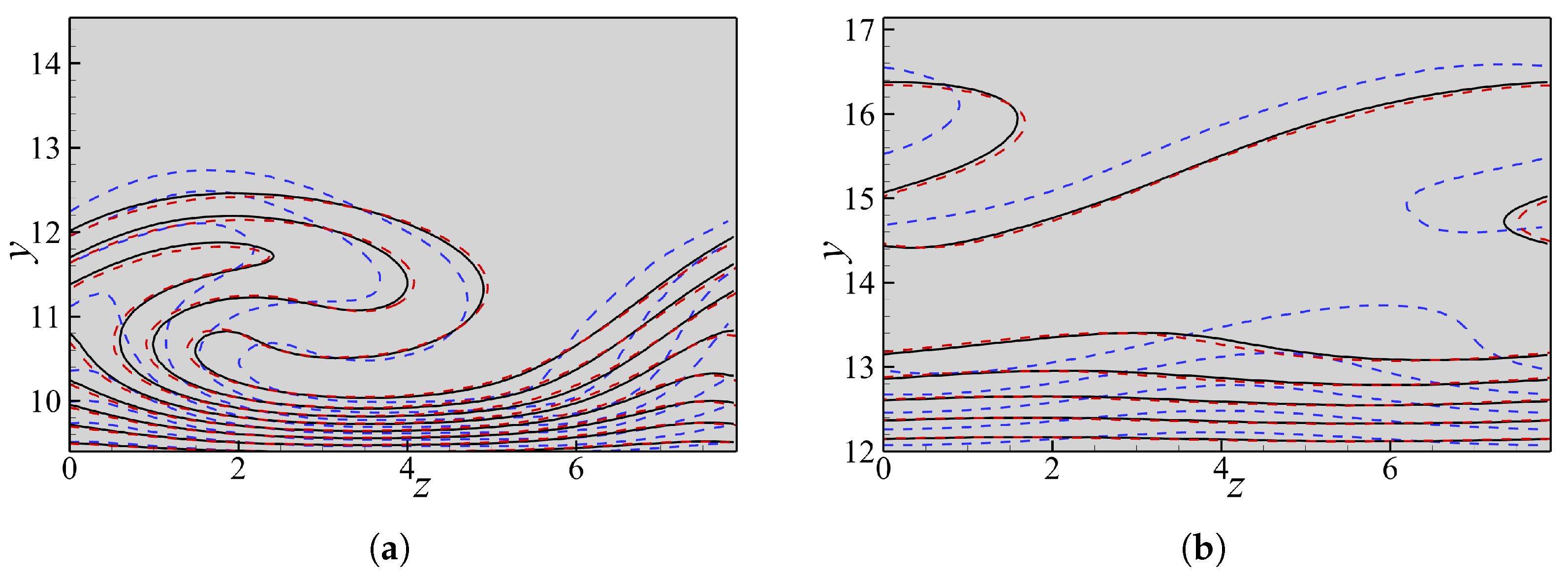
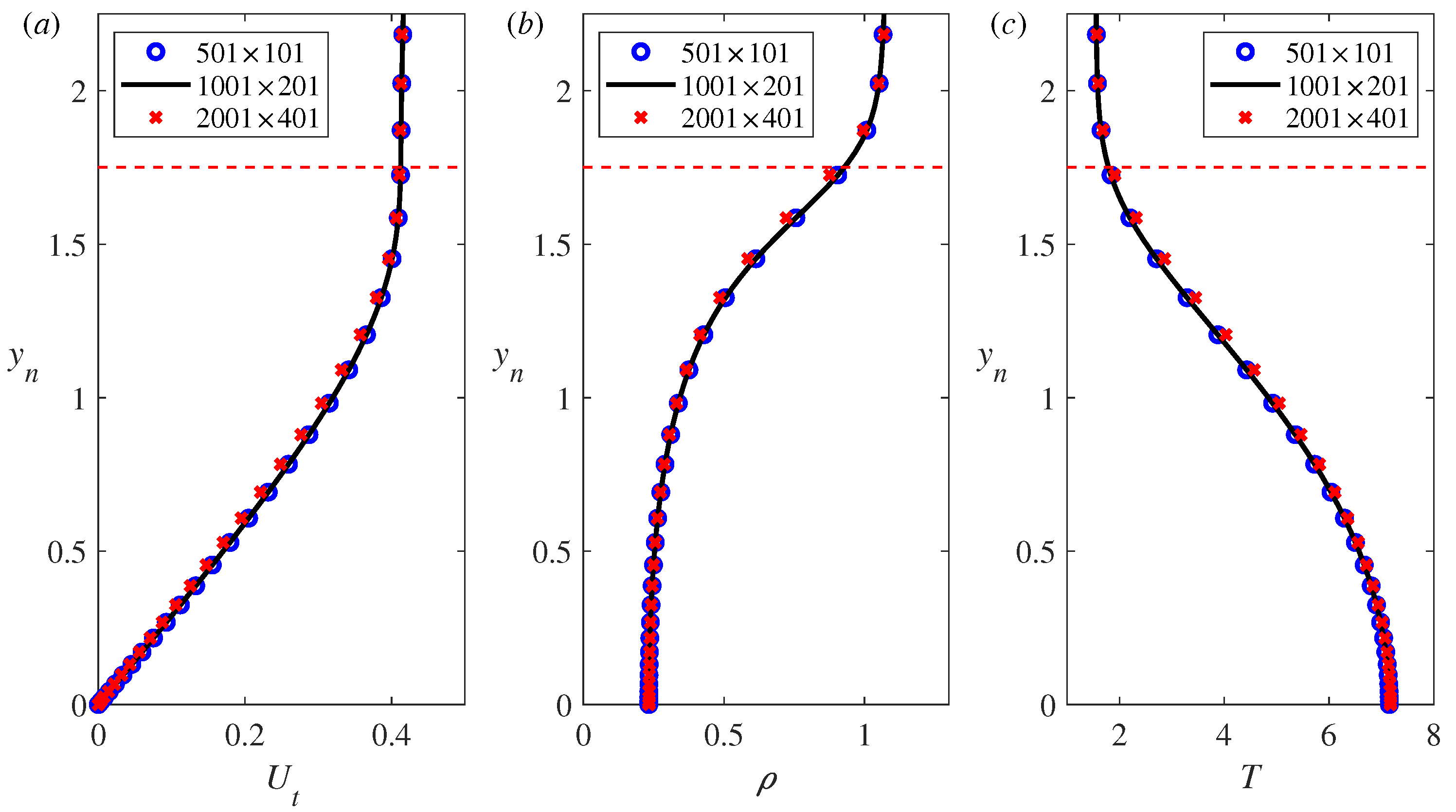
The distribution of the streamwise grid spacing and an overview of the computational grid are shown in Figure 3a. Following grid independence studies, the final mesh for the base flow computation consists of $1001\times 201$ points, as illustrated in Figure 4. For the DNS calculations, a grid with $2851\times 301\times 120$ points in the streamwise, wall-normal and spanwise directions is employed. Figure 5 presents a comparison of the crossflow vortex obtained with different meshes. It can be seen that the coarsest grid fails to adequately capture the crossflow vortex characteristics, whereas the two finer grids exhibit only minor differences. Consequently, the grid with $2851\times 301\times 120$ points is adopted for the DNS.

3. Base Flow Features

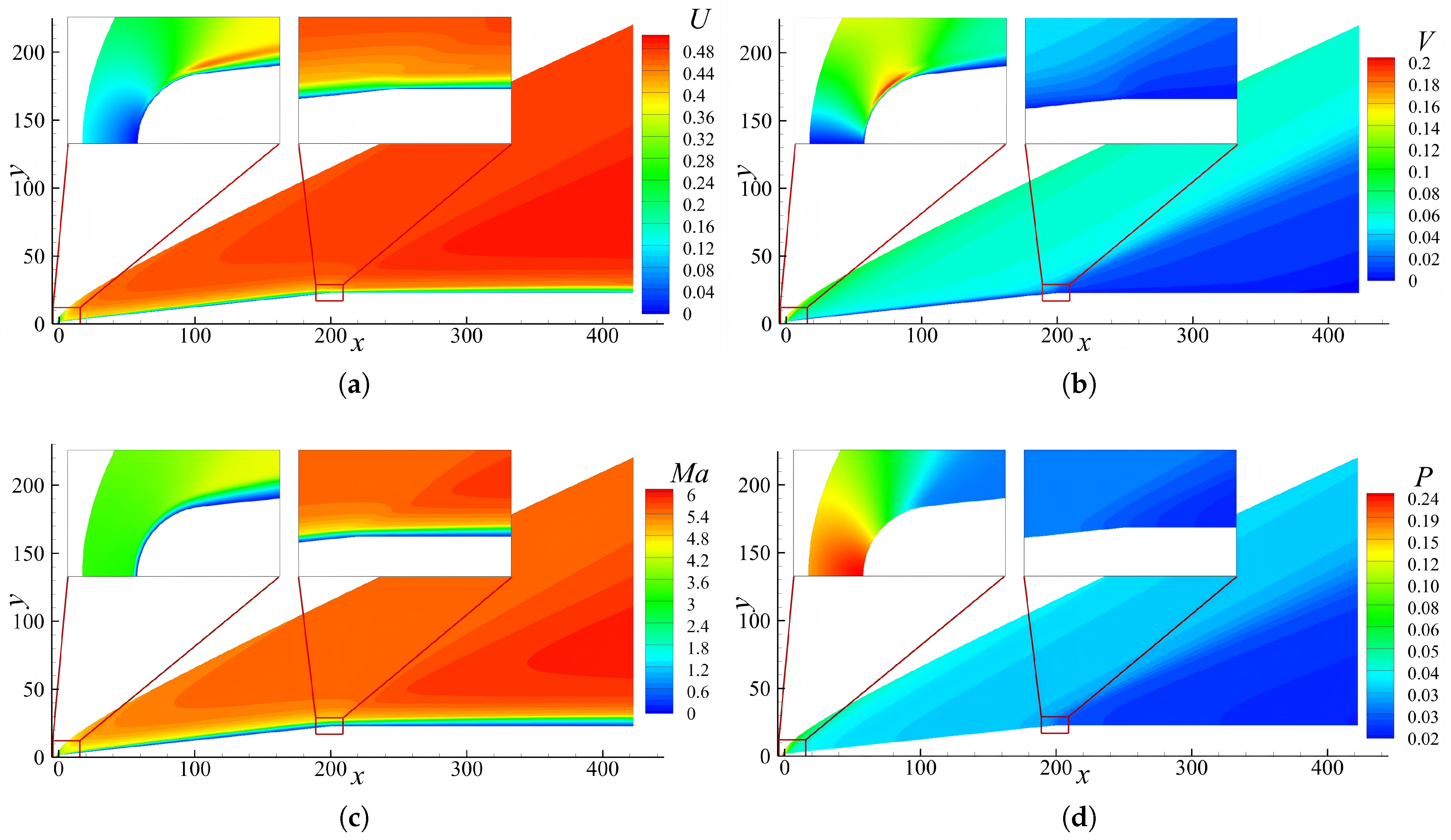
Taking the flow field with a ${60}^{\circ }$ sweep angle as an example, the overall flow structure is illustrated in Figure 6. It can be observed that the shock-fitting procedure employed in this study yields accurate flow field results, with no unphysical oscillations in the contour plots—an outcome that is often difficult to achieve with shock-capturing methods. At the expansion corner, the expansion effect leads to a reduction in boundary layer thickness, which subsequently increases downstream. Moreover, a distinct Mach wave structure generated by the expansion can be clearly seen near the wall propagating downstream from the corner.

Under the usual boundary layer approximation, the pressure is typically assumed to be constant across the boundary layer in the wall-normal direction, i.e., the $\partial p/\partial y_n$ term is neglected. However, it is worth noting that in the vicinity of the expansion corner, the pressure contours within the boundary layer are not everywhere perpendicular to the wall. At a small distance from the wall (while the pressure gradient normal to the wall is zero at the wall itself due to the boundary condition), the contour lines exhibit a distinct inclination within the boundary layer in this region, suggesting that the effects of wall-normal pressure and velocity variations should be additionally accounted for in the local boundary layer approximation.

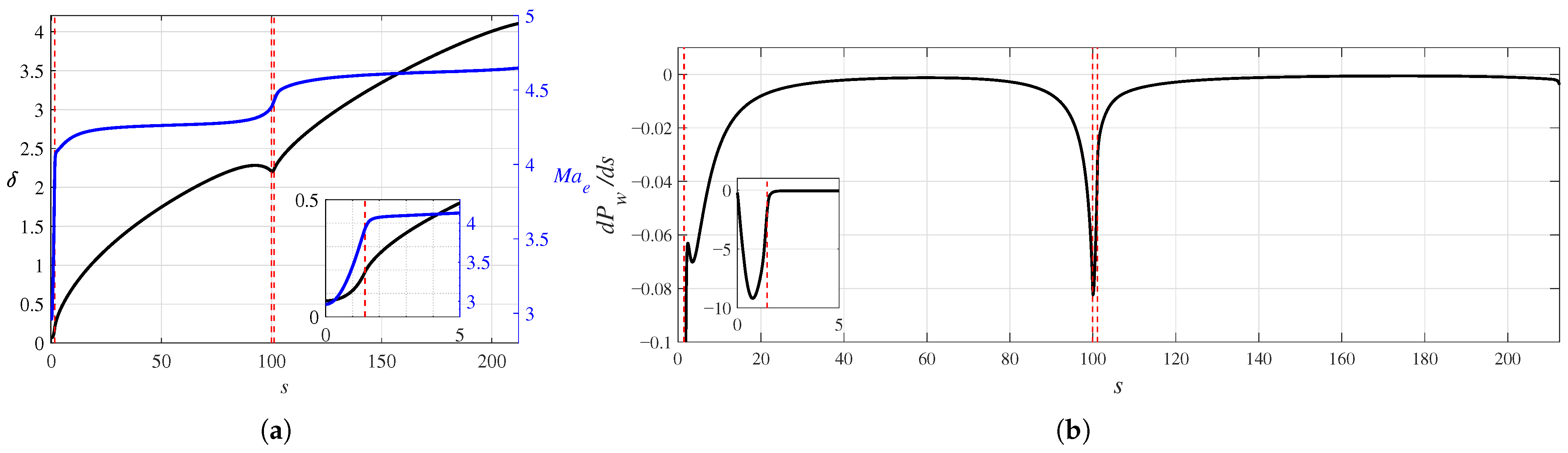
Further analysis is conducted on the streamwise variations of the flow parameters. Figure 7a presents the distributions of the boundary layer thickness and the edge Mach number for the swept wing with $\Lambda ={60}^{\circ }$. The boundary layer thickness is defined as the wall-normal distance at which the spanwise velocity reaches 99% of its freestream value, i.e., $W\left(\delta \right)=0.99W_{\infty }$. The red dashed lines in the figure indicate the locations where the surface curvature is discontinuous: the nose-wedge junction, the wedge–corner junction and the corner–plane junction. It can be seen that the boundary layer thickness begins to decrease upstream of the expansion corner, and the boundary layer accelerates under the influence of a favourable pressure gradient, becoming thinner, while the edge Mach number increases accordingly. Over most of the wedge and the flat plate, the edge Mach number exhibits only a modest increase, with significant variations confined to the nose region and the vicinity of the expansion corner. Figure 7b shows the corresponding streamwise pressure gradient. It is observed that upstream of the expansion corner, at approximately $s=70$, the pressure gradient begins to deviate from that on the wedge, giving rise to a significant favourable pressure gradient. This gradient reaches a peak value of approximately $-0.08$ for $d{P}_w/ds$ shortly after the geometric onset of the expansion corner, which is considerably smaller than the maximum pressure gradient of $-9.20$ observed at the nose. Downstream of the expansion corner, the favourable pressure gradient decreases sharply.

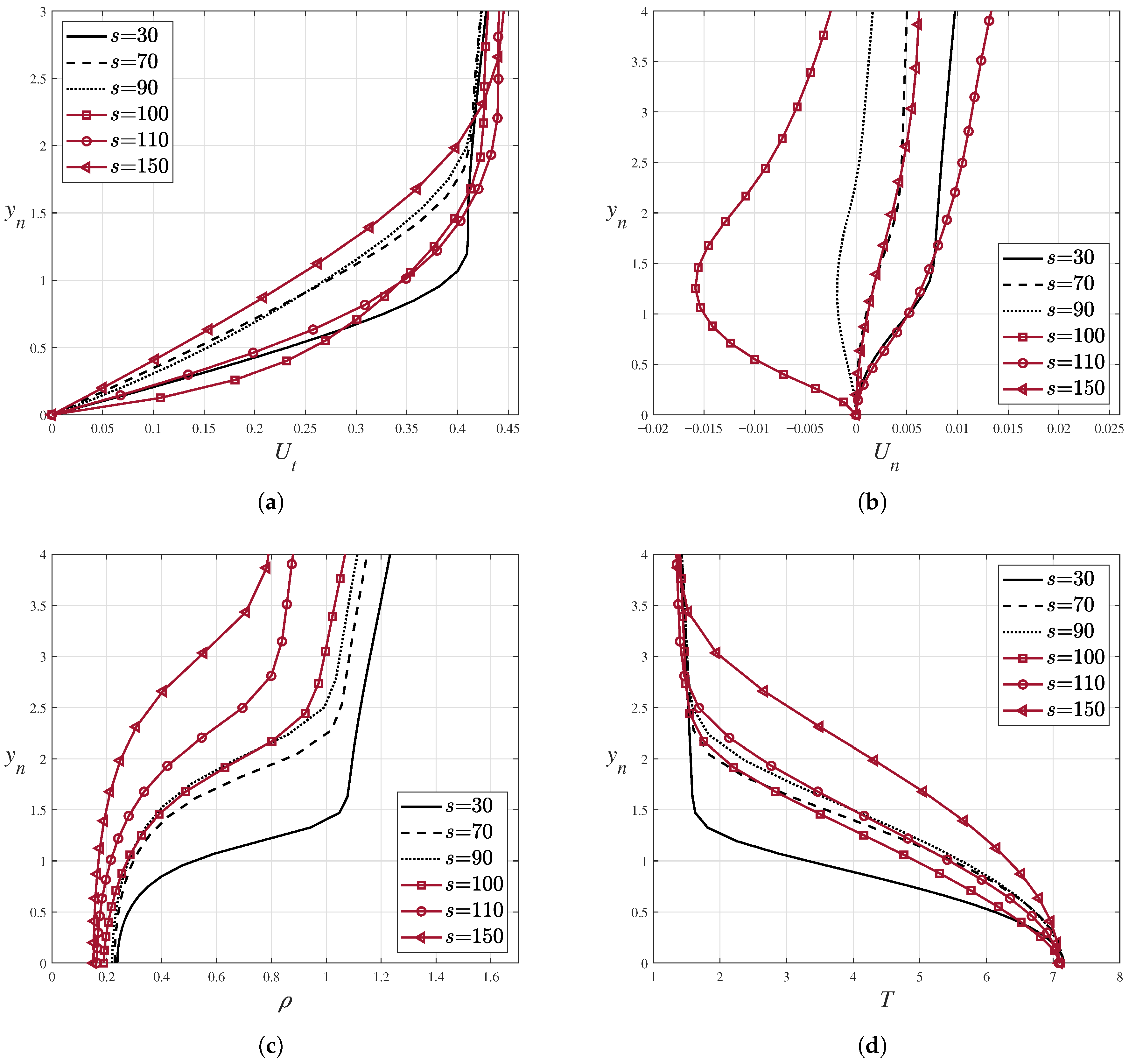
Figure 8 presents the profiles of the dimensionless velocity components tangential and normal to the wall, $U_t$ and $U_n$, together with the density $\rho$ and temperature T, at six selected locations upstream and downstream of the expansion corner for the baseline case. The first three stations, located upstream of the corner, are denoted by black lines; the remaining three, situated at and downstream of the corner, are denoted by red lines. According to Prandtl–Meyer expansion theory, in the inviscid region, the streamwise velocity increases, while the static pressure, density and temperature decrease, and the Mach number increases. From the streamwise velocity profiles shown in Figure 8a, it can be seen that, as the flow develops downstream, a distinct acceleration occurs near the wall upstream of the expansion corner (at $s=90$), leading to fuller velocity profiles. Between $s=100$ and $s=110$, the near-wall velocity decreases, whereas the velocity in the outer part of the boundary layer increases. Further downstream, at $s=150$, the overall velocity level is reduced and the boundary layer thickness has increased. The wall-normal velocity exhibits notable variations across these stations, as shown in Figure 8b. At $s=90$ and $s=100$, the wall-normal velocity becomes negative. In contrast to the classical boundary layer solution, where the wall-normal velocity is positive, the occurrence of negative values here is primarily attributed to the pressure gradient induced by the expansion corner. This implies that high-momentum fluid is transported towards the wall by the wall-normal velocity. Furthermore, as the flow evolves downstream, the density gradually decreases. The temperature, after a slight reduction near the corner, increases downstream. The wall temperature shows little variation along the streamwise direction, decreasing only slightly.

To investigate the evolution of the three-dimensional boundary layer in this study, it is necessary to examine several key flow quantities commonly used in crossflow analyses. First, the velocity vector is decomposed into a component aligned with the inviscid flow direction at the boundary layer edge and a component perpendicular to it, i.e., the crossflow. Specifically, the angle between the edge velocity direction and the streamwise direction s is denoted by ${\theta }_e$, where ${\theta }_e=arctan(W_e/U_e)$, with the subscript e denoting quantities at the boundary layer edge. The velocity within the boundary layer can then be decomposed with respect to the inviscid flow angle as:

$$\left\{\begin{array}{c}{U}_{pf}=Ucos{\theta }_e+Wsin{\theta }_e,\hfill \\ U_{cf}=-Usin{\theta }_e+Wcos{\theta }_e,\hfill \end{array}\right.$$

(10)

where $U_{pf}$ is the velocity component aligned with the potential flow direction and $U_{cf}$ is the crossflow velocity component.

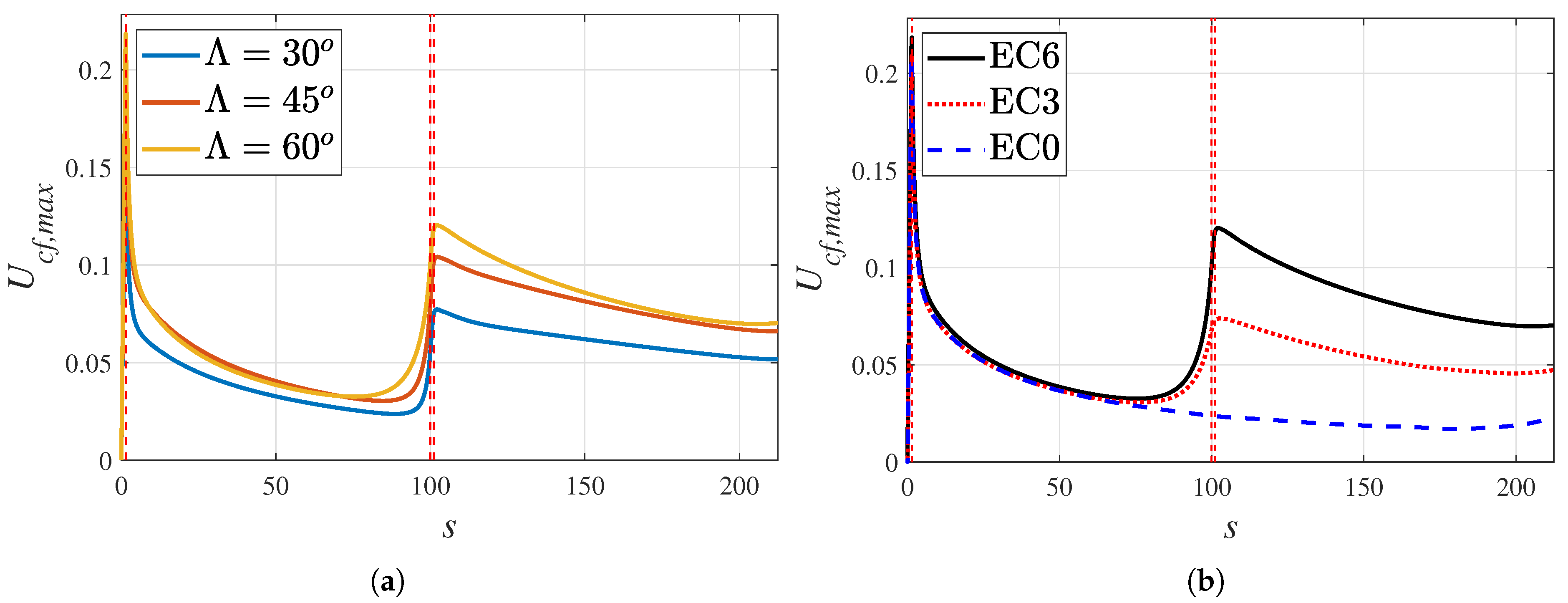
Figure 9 presents the streamwise development of the maximum crossflow velocity within the flow cross-section under different conditions. It can be observed that peaks in the maximum crossflow velocity occur at both the nose and the expansion corner, with the crossflow velocity already increasing upstream of the expansion corner. A larger sweep angle corresponds to a larger inviscid flow angle, which intensifies the imbalance between the centrifugal force and the pressure gradient within the boundary layer, thereby strengthening the crossflow. As the expansion corner angle increases, the crossflow also tends to become more pronounced.

4. Linear Evolution Features

4.1. Eigenmode Characteristics

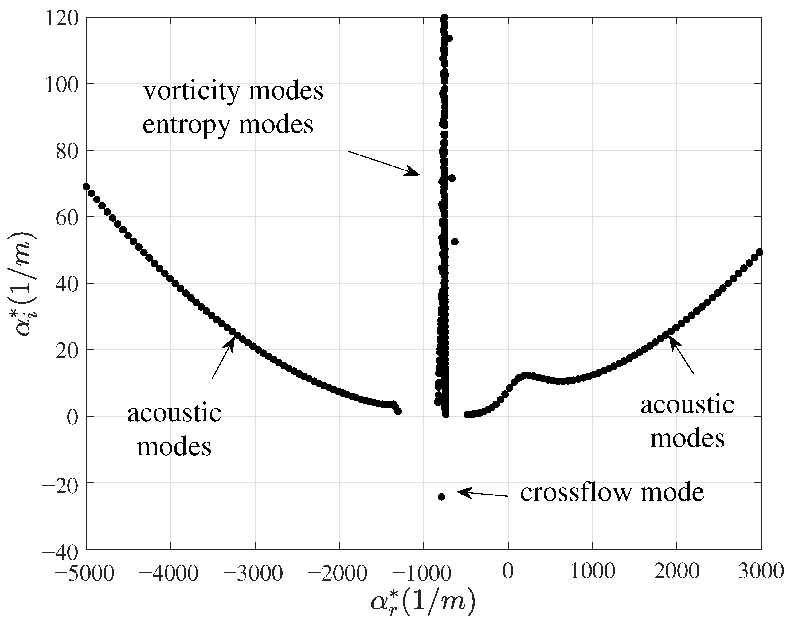
For the base flow over the swept wing with an expansion corner discussed in the preceding section, the computed eigenvalue spectrum and the characteristics of the unstable modes are first presented. Figure 10 shows the eigenvalue spectrum of the stationary (i.e., $\omega =0$) modes at $s=20$, with a spanwise wavelength of 16 mm. In the eigenvalue spectrum, the continuous spectra of acoustic, vorticity and entropy waves can be clearly distinguished [8]. In the unstable region, only one unstable disturbance is observed.

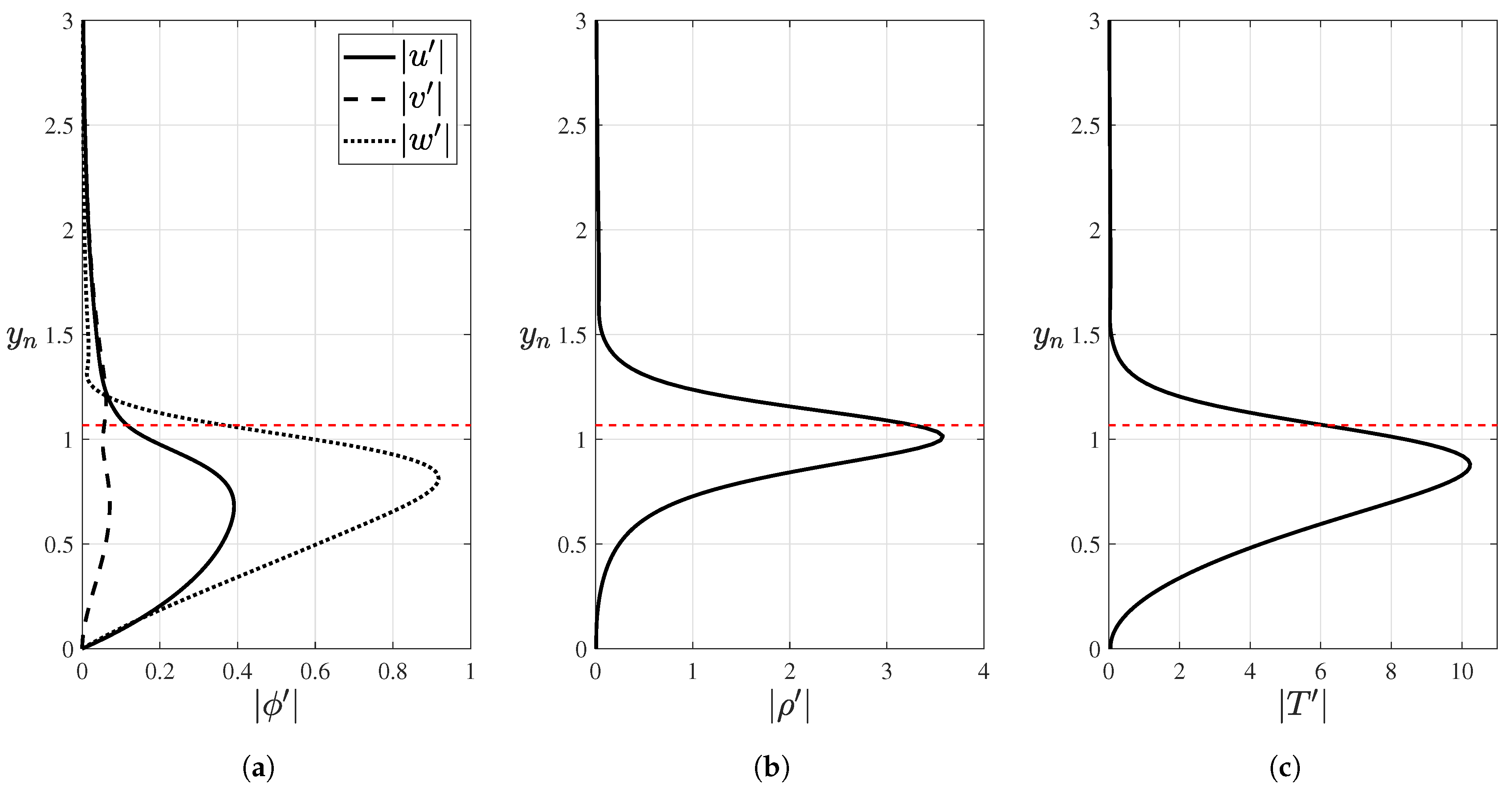
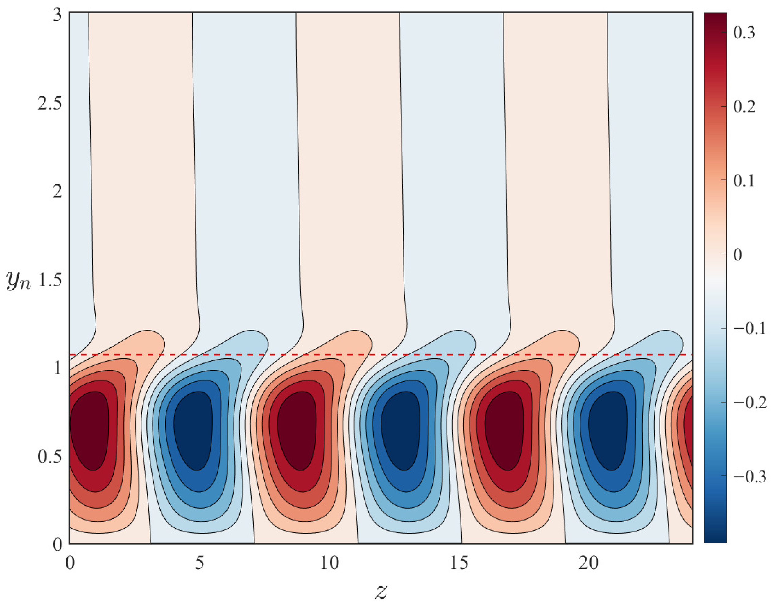
Figure 11 presents the disturbance eigenfunction profiles for this unstable mode, with the boundary layer thickness indicated by the red dashed line. In addition, Figure 12 shows the reconstructed spanwise–wall-normal contours of the velocity disturbances. Note that the contour levels represent normalized amplitudes, and the horizontal axis z corresponds to the spanwise spatial coordinate. It can be observed that this mode exhibits distinct characteristics of a crossflow instability, with the peak disturbance velocity located in the upper part of the boundary layer, consistent with the location of the maximum crossflow velocity. In contrast to the velocity disturbances, the density and temperature disturbances attain their maxima very close to the boundary layer edge. Among the velocity components, the spanwise disturbance velocity $w^{\prime }$ is considerably larger than the disturbance velocities in the other two directions.

Neutral Curves

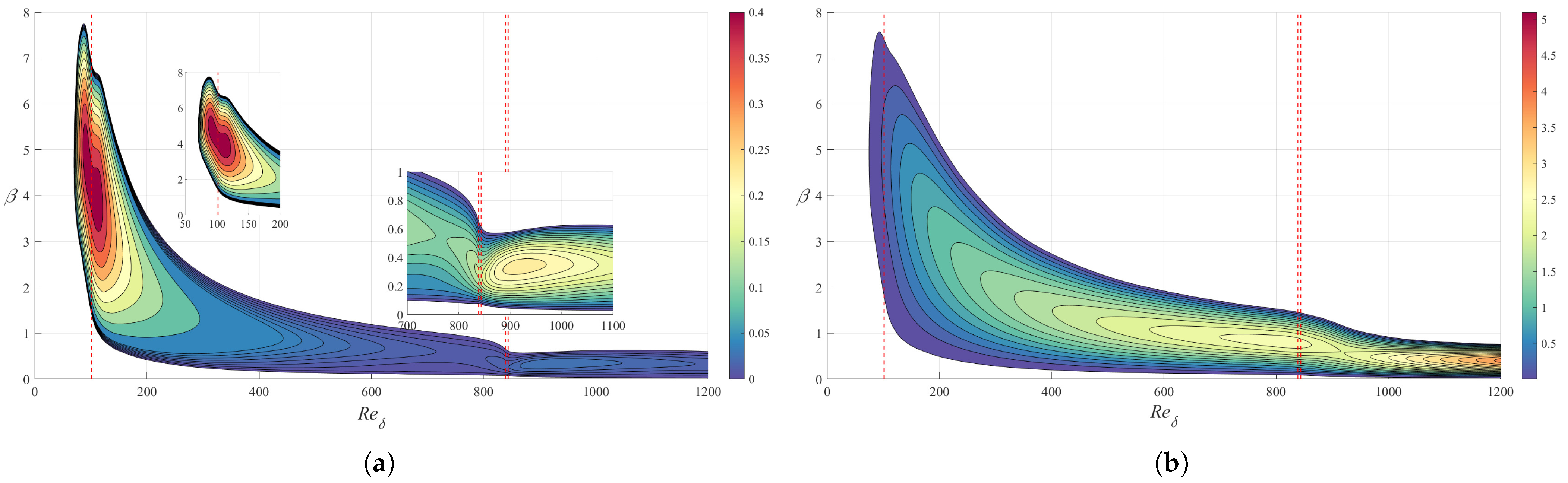
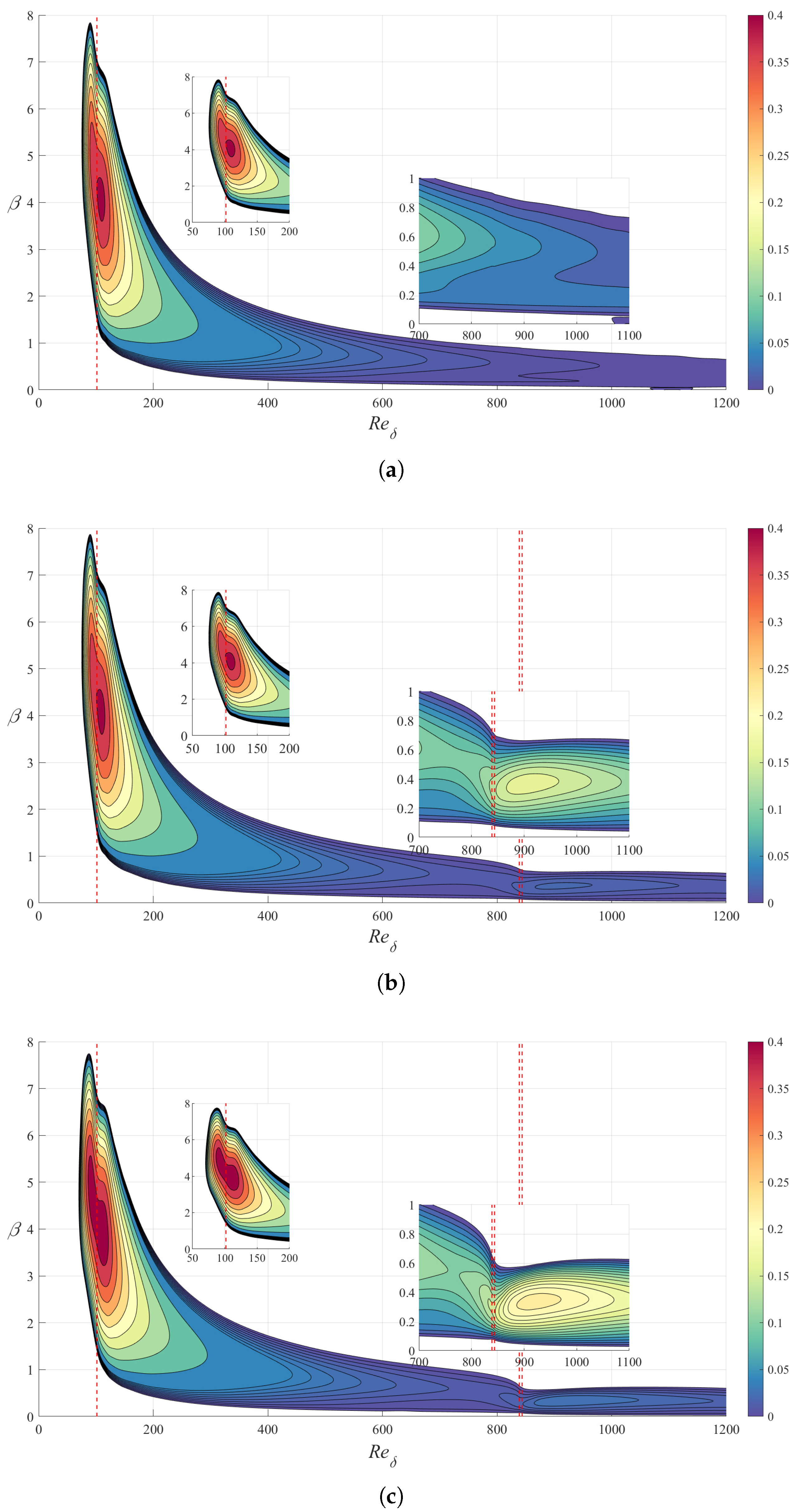
To further investigate the stability characteristics of the flow, Figure 13 presents the linear stability neutral curve for the sweep angle of ${60}^{\circ }$, with $R{e}_{\delta }=U_{\infty }\delta /{\nu }_{\infty }$ the Reynolds number based on the boundary layer thickness scale $\delta =\sqrt{{\nu }_{\infty }{s}^{*}/U_{\infty }}$. The ordinate denotes the spanwise wavenumber $\beta ={\beta }^{*}·R^{*}$, with $R^{*}$ refers to the dimensional leading-edge radius, and the spanwise wavelength ${\lambda }_z={\lambda }_z^{*}/R^{*}$. The critical Reynolds number is approximately 70. When the streamwise Reynolds number reaches approximately 840, the flow traverses the expansion corner, downstream of which a new peak in the growth rate can be observed. Figure 13b shows the distribution of the N factor obtained by integrating the growth rates. The first peak occurs at a local Reynolds number of approximately 810, while a second peak is observed near the downstream exit. The first peak corresponds to a spanwise wavelength of approximately 8, whereas the second peak corresponds to a wavelength of approximately 16. The dominant mode downstream of the corner, with a wavelength of 16, is precisely the subharmonic of the dominant ${\lambda }_z=8$ mode upstream of the corner. These two particular modes will be further investigated in the subsequent analysis of nonlinear evolution and secondary instability. The above observations indicate that the expansion corner further amplifies the crossflow instability within the boundary layer, with the subharmonic of the originally dominant crossflow mode becoming predominant downstream.

Theoretical and experimental studies generally suggest that expansion waves exert a stabilizing influence on the flow. Chuvakhov [25] conducted a linear stability analysis of a hypersonic two-dimensional expansion corner and found that, in the absence of sweep, the second mode is dominant. The primary effect of the expansion corner on the stability characteristics is mediated by the increase in boundary layer thickness, which significantly reduces the frequency of the second-mode disturbances. The growth rates of high-frequency modes drop sharply at the expansion corner, while previously stable low-frequency modes become unstable, ultimately rendering the flow more stable.

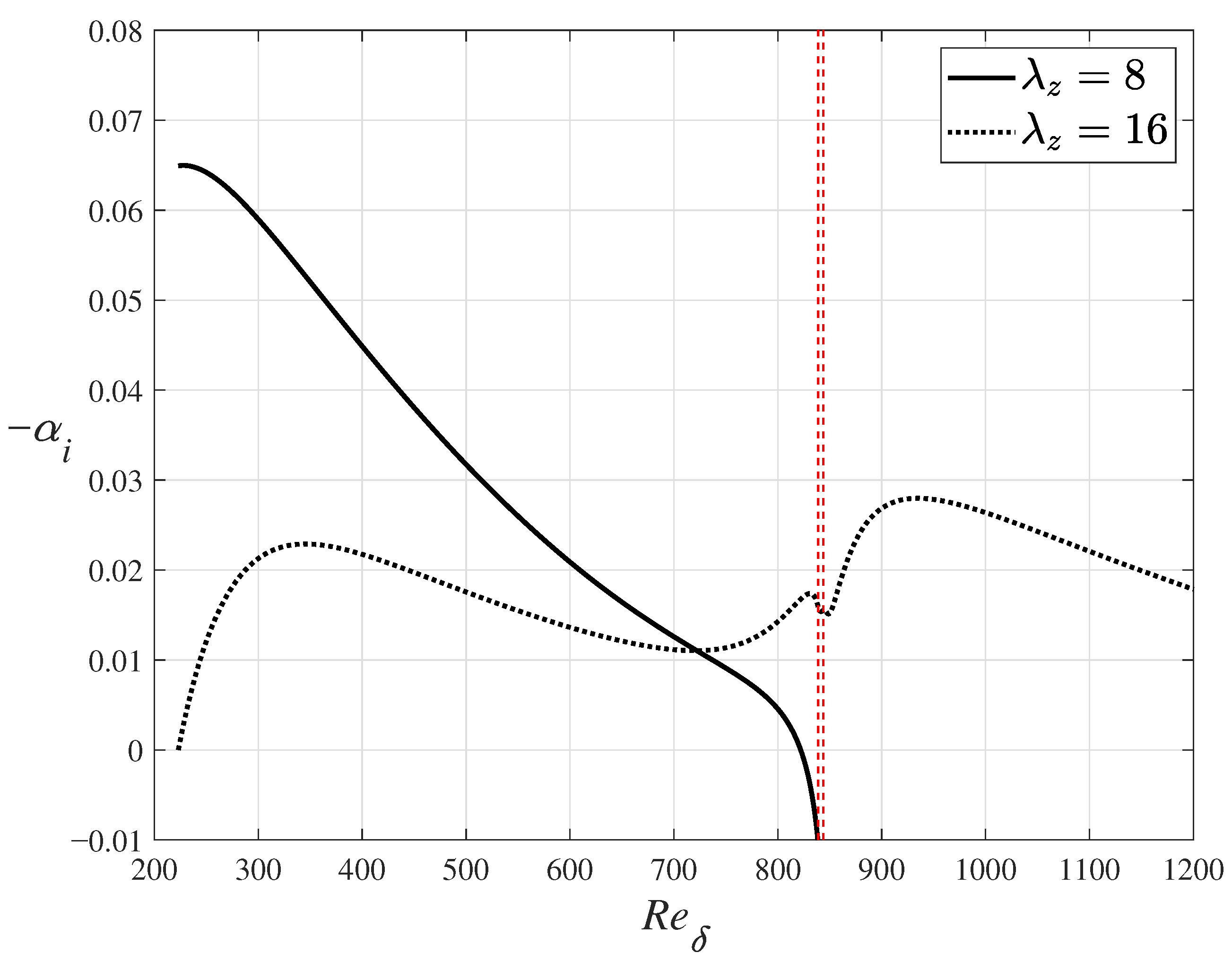
In contrast, the present local linear stability analysis yields a different conclusion for the stationary crossflow mode. As shown in Figure 14, on the wedge surface downstream of the nose, the growth rate of the unstable crossflow mode gradually decreases as the boundary layer develops downstream. As the flow traverses the expansion corner, the base flow quantities such as density and temperature undergo significant changes in their distributions, and the maximum crossflow velocity increases markedly, rendering the crossflow mode more unstable. The spanwise wavenumber of the most unstable mode in this region differs considerably from the previously dominant one, with a wavelength approximately twice that of its upstream counterpart. On the flat plate downstream of the expansion corner, as the boundary layer continues to develop downstream, the disturbance growth rate decreases once again.

Figure 15 presents the neutral curves for different sweep angles. It is evident from the figure that as the sweep angle increases, the crossflow instability is enhanced overall. This enhancement is first manifested in a reduction of the critical Reynolds number: as the sweep angle increases from ${30}^{\circ }$ to ${60}^{\circ }$, the critical Reynolds number decreases from approximately 105 to about 70. Furthermore, the maximum growth rate is also increased; the maximum growth rate for the ${30}^{\circ }$ sweep case is almost an order of magnitude smaller than that for the ${60}^{\circ }$ sweep case. In addition to the overall increase in disturbance growth rates, the neutral curves also reveal that, with increasing sweep angle, the spanwise wavenumber of the most unstable disturbance decreases, implying an increase in the spanwise wavelength. Moreover, the bandwidth of unstable spanwise wavenumbers within the unstable region is also reduced.

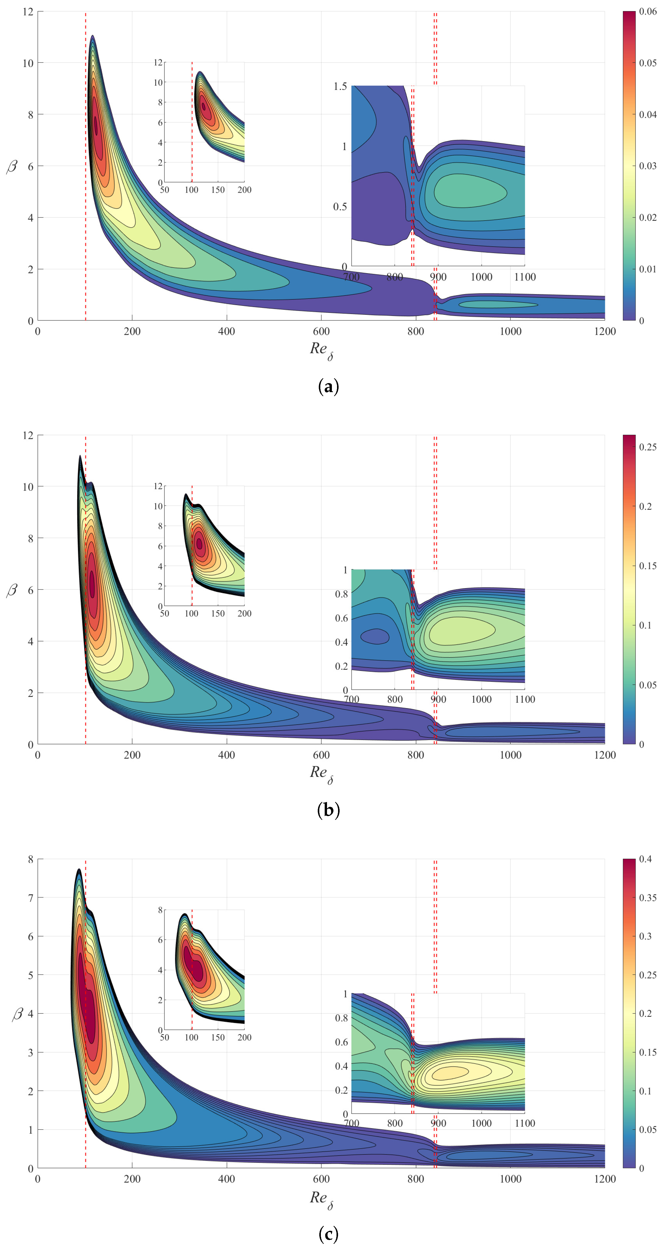
Figure 16 shows the neutral curves for different expansion corner angles. It can be seen that, up to a local Reynolds number of approximately 700, the results for the three cases are nearly identical. For local Reynolds numbers greater than 700, the stationary crossflow mode gradually decays in the case without an expansion corner, whereas a significant destabilisation is observed for both the $3^{\circ }$ and $6^{\circ }$ expansion corner cases. The enhancement becomes more pronounced as the corner angle increases. The locations of the maximum disturbance growth rates are almost the same for all cases. Overall, a stronger expansion effect leads to larger disturbance growth rates downstream of the corner, accompanied by smaller spanwise wavenumbers.

Based on the results obtained from LST, the two most relevant disturbance modes for the present case correspond to spanwise wavelengths of 8 and 16, respectively. According to LST predictions, the amplitude of the ${\lambda }_z=8$ mode reaches its maximum upstream of the expansion corner, while that of the ${\lambda }_z=16$ mode attains its maximum downstream of the corner. It is worth noting that the linear stability analysis presented above neglects non-parallel effects such as curvature and boundary layer growth. In the vicinity of the expansion corner in particular, this assumption may lead to substantial discrepancies between the predicted and actual disturbance growth. To further investigate the linear stability of stationary crossflow modes on swept wing configurations with an expansion corner, accounting for non-parallel effects, direct numerical simulations are required.

4.2. Linear DNS Analysis

For the base flow obtained from the shock-fitting procedure described above, the inflow boundary is placed at $s=20$. The unstable modes predicted by LST are superimposed onto the basic flow as initial disturbances for the DNS. The disturbance amplitude is defined as the ratio of the maximum streamwise disturbance velocity to the freestream velocity. To satisfy the small-disturbance assumption, the amplitude is set to $1\times {10}^{-5}$ in all cases. Since the disturbances of interest are stationary crossflow modes, time-accurate DNS is performed and marched until the flow field converges to a steady state. After obtaining the converged flow fields, a spatial Fourier decomposition is performed in the spanwise direction to extract the fundamental spanwise harmonic, which is then compared with the LST results.

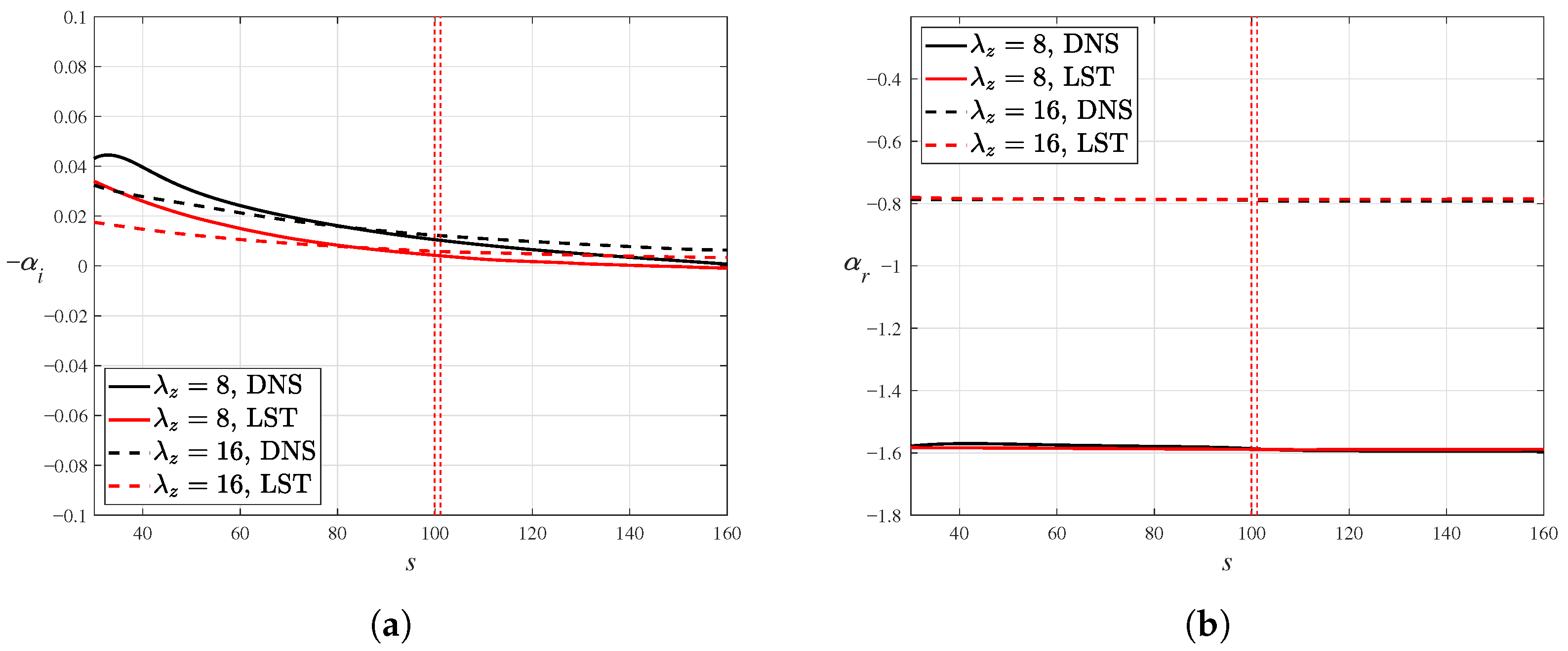
First, the DNS results for the case without an expansion corner are compared with the LST predictions. Figure 17 presents a comparison of the streamwise wavenumber and growth rate of the disturbance extracted from the DNS flow field with the corresponding eigenmode properties obtained from LST for the ${60}^{\circ }$ swept configuration without an expansion corner. It can be seen that the streamwise wavenumber obtained from the DNS is in good agreement with the LST result. However, the disturbance growth rate computed from the DNS is significantly larger than that predicted by LST.

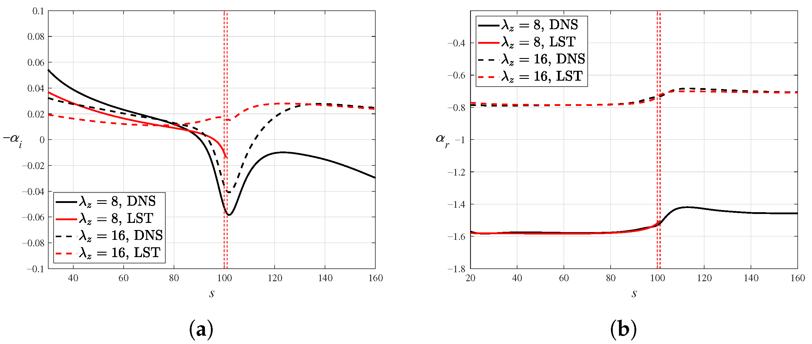
Next, the DNS results for the case with an expansion corner are compared with the LST predictions. The configuration analysed here features a $6^{\circ }$ expansion corner. Figure 18 shows a comparison of the growth rate and streamwise wavenumber. As previously observed for the case without an expansion corner, the growth rates obtained from DNS are higher than those predicted by LST upstream of the expansion corner. As the flow approaches the expansion corner, the growth rate predicted by DNS decreases rapidly, reaching a minimum at the corner itself. For the ${\lambda }_z=16$ case, the growth rate downstream of the corner returns to values consistent with the LST predictions. For the ${\lambda }_z=8$ case, however, the LST-predicted mode lies in a stable region downstream of the corner and heavily overlaps with the continuous spectrum, making it difficult to track. Therefore, only the DNS results are shown for this case. The DNS exhibits a trend similar to that observed for the ${\lambda }_z=16$ case, except that the disturbance growth rate remains negative downstream of the corner, indicating that the disturbance continues to decay. The difference between the results of the LST and DNS indicates that the LST is not valid between $s=80$ and $s=130$.

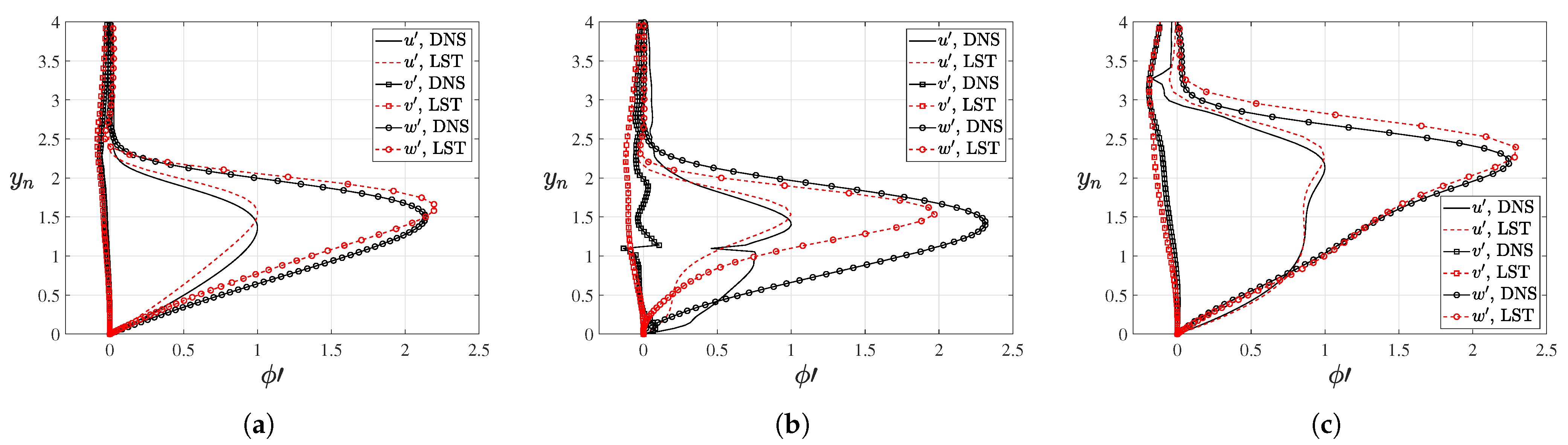
The disturbance profiles extracted at $s=80$, 100 and 140 are shown in Figure 19. At the expansion corner, i.e., at $s=100$, a localized discontinuity is observed in the DNS disturbances, which is attributed to the $C^2$ discontinuity of the surface geometry at the junction of the expansion corner, which can only be captured by DNS. Further downstream, the DNS disturbances are again in agreement with the LST results. The eigenfunction structure of the ${\lambda }_z=16$ mode changes across the expansion corner: the $u^{\prime }$ profile downstream of the corner exhibits two peaks, whereas upstream it exhibits only one. This change in eigenfunction structure ultimately leads to an increase in its growth rate.

Based on the above analysis, it can be concluded that, when non-parallel effects (including boundary layer growth, wall-normal pressure gradients, wall curvature, etc.) are taken into account, the disturbance growth rate undergoes a sharp decrease at the expansion corner. Upstream and downstream of the corner, however, the overall trend of the disturbance growth rate remains consistent with the LST predictions. At the expansion corner itself, local LST fails because it neglects non-parallel effects—in particular, the wall-normal pressure gradient and momentum transport induced by the expansion. Therefore, it is necessarily invalid in the vicinity of the corner, and approaches such as DNS, which incorporate a comprehensive set of physical factors, are required to properly capture the disturbance evolution in this region.

5. Nonlinear Evolution Features

5.1. Fundamental Disturbance Evolution

Based on the linear stability analysis presented in the previous section, the disturbance characteristics most likely to evolve into the stationary crossflow vortices observed in natural transition of hypersonic boundary layers have been identified. The focus of the present study is not on the receptivity mechanism of crossflow modes, but rather on the influence of the expansion corner on their linear and nonlinear stability. Therefore, a DNS approach is designed such that the stationary crossflow vortices reach saturation upstream of the expansion corner while maintaining a sufficient amplitude, enabling an investigation of the effect of the expansion corner on the nonlinear interactions among disturbances and on the development of crossflow vortices. Furthermore, since crossflow transition is typically triggered by high-frequency secondary instabilities of saturated crossflow vortices, it is important to examine the impact of the expansion corner on secondary instability.

To investigate the effect of the expansion corner on fully developed crossflow vortices, extensive trial computations were performed. It was ultimately determined that, for the case with ${\lambda }_z=8$ disturbances, the inflow amplitude is set to 5%, whereas for the ${\lambda }_z=16$ case, the inflow amplitude is set to 10%.

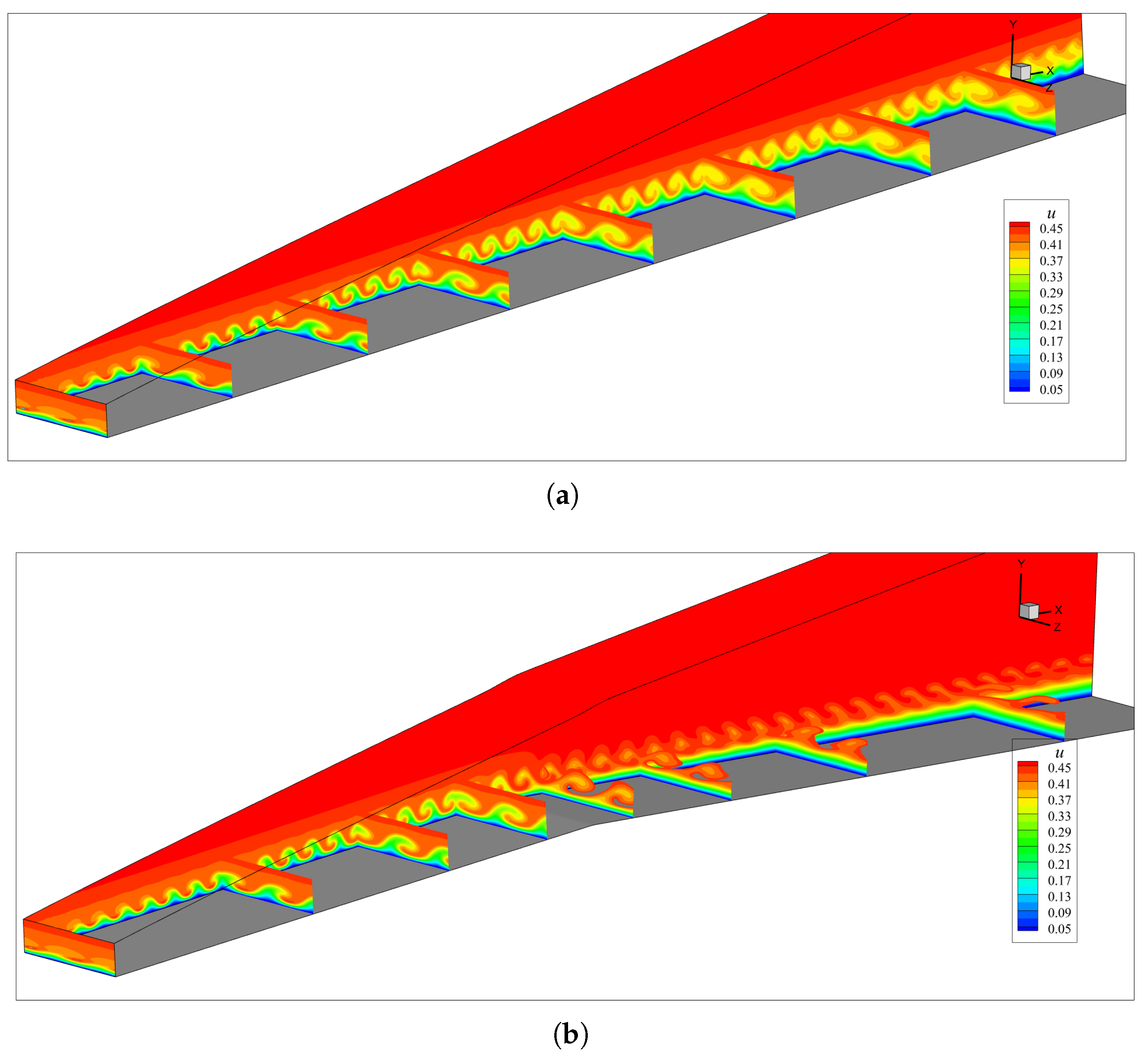
The nonlinear evolution of stationary crossflow vortices with a spanwise wavelength of ${\lambda }_z=8$ is first analysed. After introducing large-amplitude initial disturbances, the streamwise velocity contours for the two expansion corner configurations are shown in Figure 20. The crossflow vortex structures resulting from nonlinear evolution can be clearly observed in the figure. For the case without an expansion corner, the crossflow vortices continue to develop downstream. In contrast, for the case with an expansion corner, the crossflow vortices are significantly weakened downstream of the corner, which is qualitatively consistent with the conclusions drawn from the linear stability analysis.

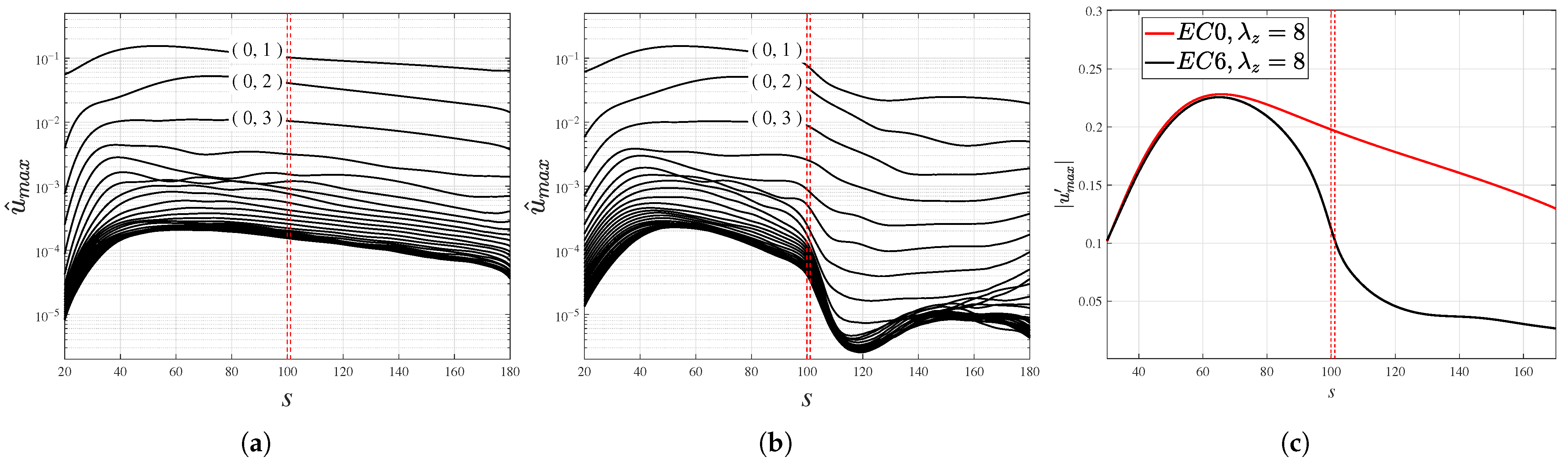
To examine the growth behaviour of the fundamental wave and its harmonics, a Fourier transform is performed on the flow field to extract the disturbance growth characteristics at various spanwise wavenumbers. Here, the maximum streamwise velocity at each spanwise wavenumber is taken as a measure of the disturbance amplitude. The streamwise evolution of these disturbance amplitudes is shown in Figure 21. In the figure, (0, 1) denotes the Fourier mode corresponding to zero temporal frequency and a spanwise wavenumber equal to $2\pi /{\lambda }_z$. It can be seen that the amplitude of the (0, 1) mode in both cases is nearly identical upstream of the corner. For higher-order modes, however, the influence of the expansion corner becomes apparent earlier than predicted by LST. At the expansion corner itself, the amplitudes of all modes decrease. Downstream of the corner, the amplitudes of the higher-order modes increase noticeably, and the overall amplitude decay is moderated, although the intensity of the crossflow vortices observed in the contours is substantially reduced.

The streamwise development of the overall disturbance streamwise velocity is shown in Figure 21c. It is evident from the figure that, although the two configurations are geometrically identical upstream of the corner, the nonlinear evolution of the disturbances differs at an early stage. Based on the analysis in previous sections, this indicates that even weak pressure gradient variations have a significant impact on the nonlinear evolution of stationary crossflow vortices. In both cases, the disturbance amplitude reaches a peak between $s=60$ and $s=70$, after which the saturated stationary crossflow vortices begin to decay. The decay is more rapid in the case with an expansion corner. As shown in Figure 21, the subsequent disturbance growth involves two stages. First, at approximately $s=120$ downstream of the corner, high-wavenumber modes are excited by the expansion effect; however, at this stage, the higher-amplitude modes such as (0, 1) and (0, 2) are still decaying, so the overall decay is merely slowed. Then, at $s=150$, the growth of the high-wavenumber modes levels off, while the low-wavenumber modes exhibit a weak recovery, though the overall disturbance amplitude continues to decrease. Compared with the linear small-disturbance DNS results discussed earlier, some signs of disturbance growth are observed downstream of the expansion corner in the present nonlinear case. Nevertheless, the overall trend remains consistent with the small-disturbance scenario: the disturbance amplitude continues to decrease, and the expansion corner weakens the intensity of the crossflow vortices associated with the mode that is dominant upstream of the corner.

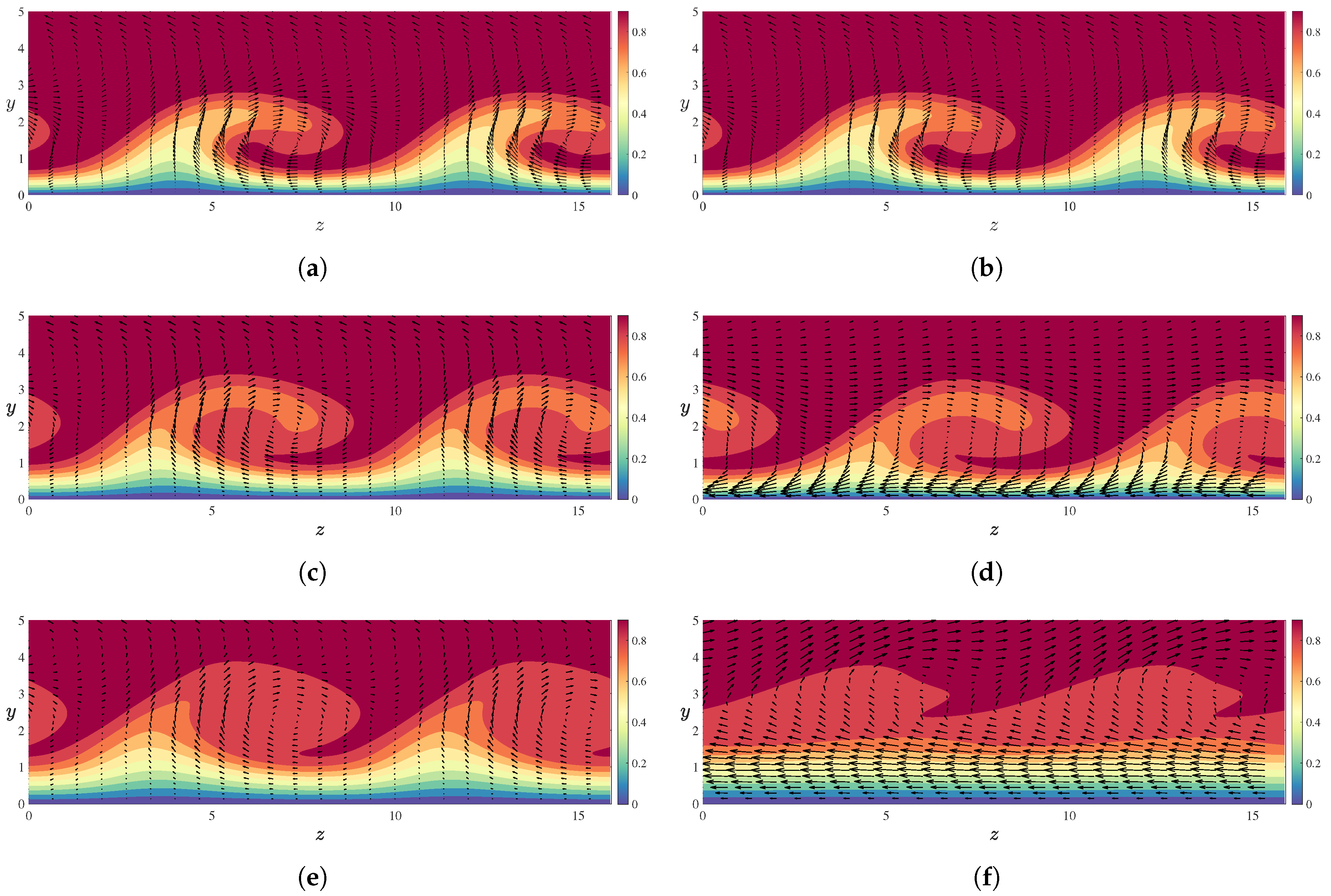
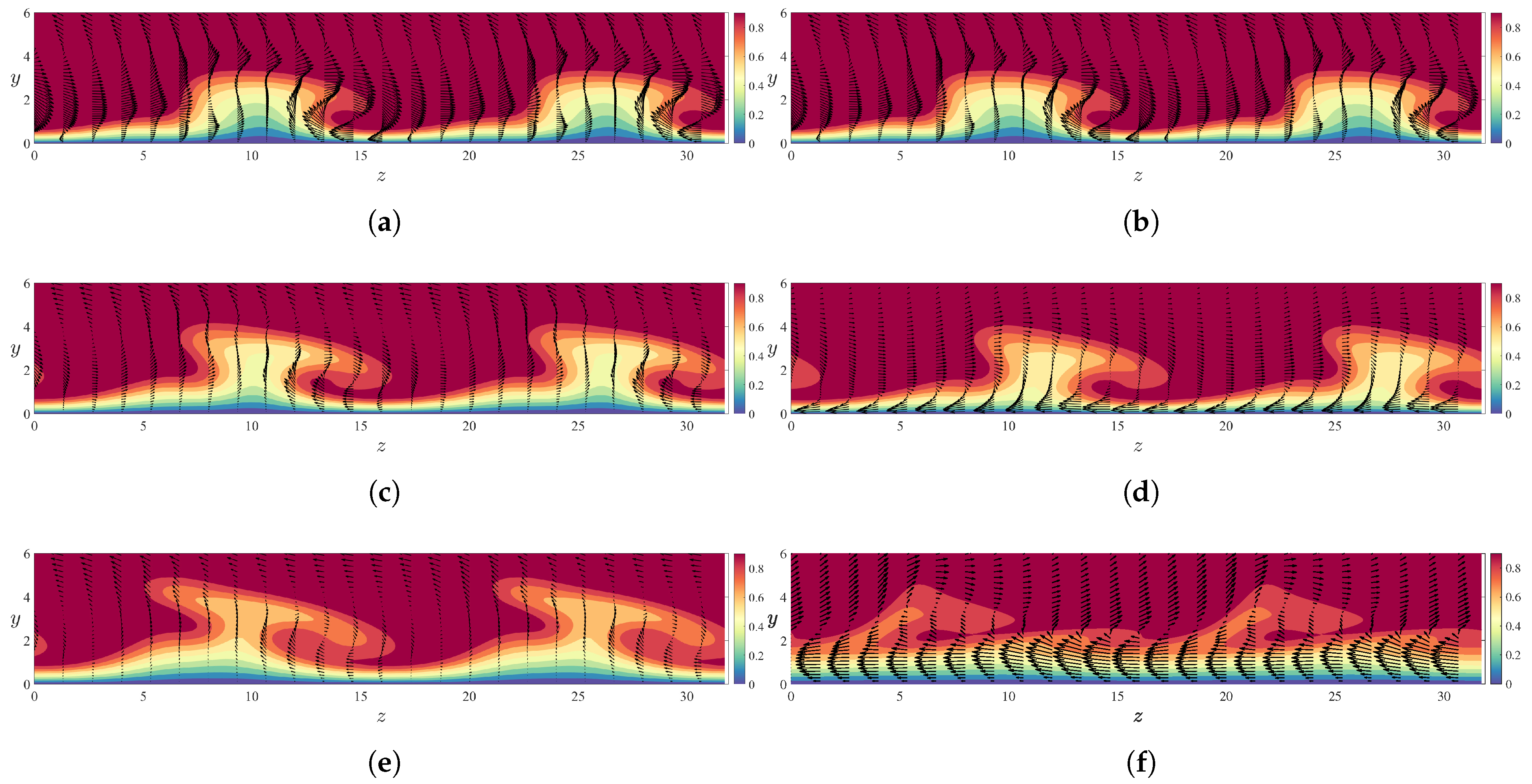
The flow field is transformed into the coordinate system aligned with the crossflow vortex axis, and the vortex velocity contours $u_v$ in the plane normal to the vortex axis are shown in Figure 22. Typical crossflow vortex structures, characterised by the upward and downward motions sweeping high-momentum fluid towards the wall and lifting low-momentum fluid away from it, are clearly observed, forming a series of co-rotating vortices. This structure is referred to as ‘rollover’ [1] or a ‘semi-mushroom’ structure [11]. In the absence of an expansion corner, the crossflow vortices grow in size as they develop downstream, with the associated lift-up and sweep-down effects becoming increasingly pronounced. In contrast, when an expansion corner is present, the crossflow vortex structures are significantly weakened; the favourable pressure gradient reduces the vortex intensity, and by $s=130$ downstream of the corner, the characteristic features of the crossflow vortices have almost entirely disappeared.

5.2. Subharmonic Disturbance Evolution

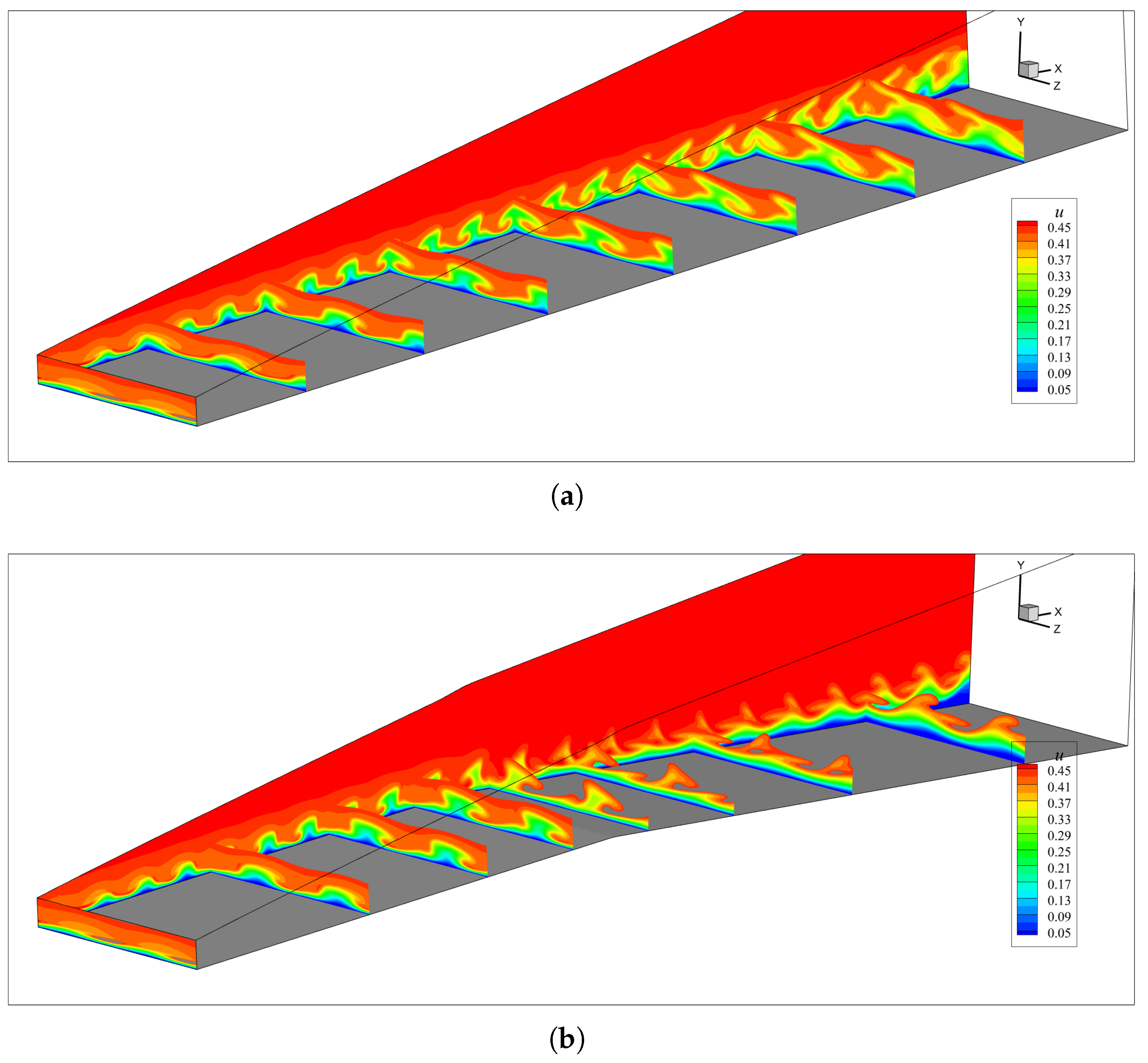
The nonlinear evolution of stationary crossflow vortices with a spanwise wavelength of 16 is now analysed. After introducing large-amplitude initial disturbances, the streamwise velocity contours for the two expansion corner configurations are shown in Figure 23. The crossflow vortex structures resulting from nonlinear evolution can again be clearly observed in the figure. However, their characteristics differ significantly from those of the ${\lambda }_z=8$ stationary crossflow vortices that are dominant upstream of the corner. For the case without an expansion corner, the crossflow vortices continue to develop downstream. In contrast, for the case with an expansion corner, the crossflow vortices are substantially weakened downstream of the corner. Nevertheless, they sustain a finite amplitude without further decay further downstream, resulting in a flow structure distinctly different from that observed in the configuration without a corner.

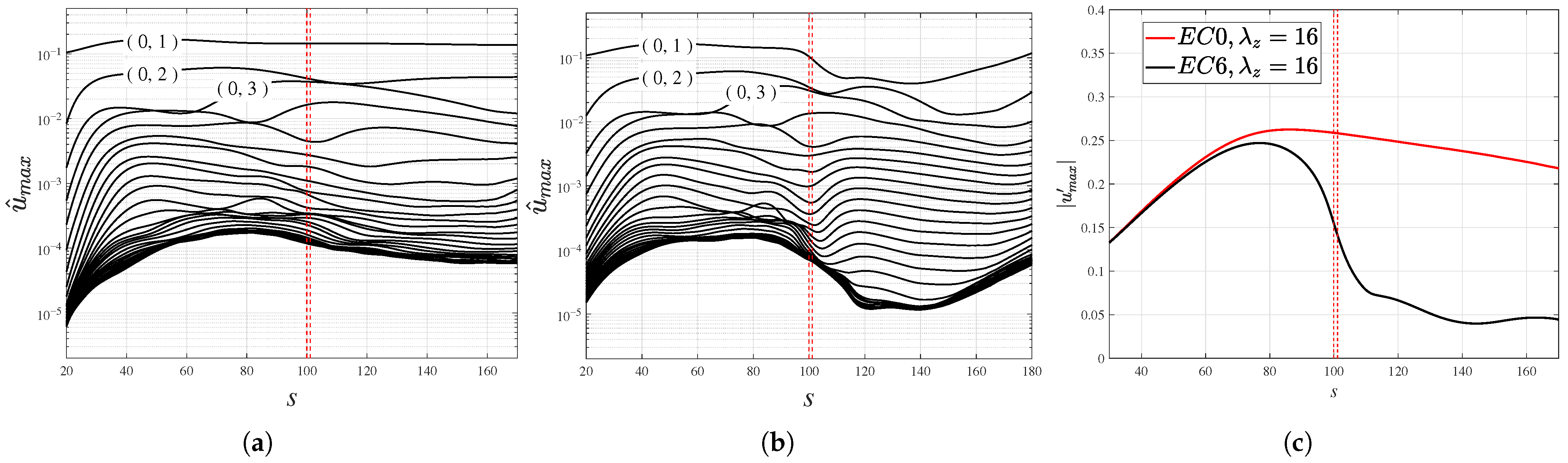
The disturbance growth characteristics at various spanwise wavenumbers are extracted by performing a Fourier transform on the flow field. The streamwise evolution of these disturbance amplitudes is shown in Figure 24. It can be observed that, upstream of the corner, the amplitudes of the dominant spanwise modes are nearly identical for both configurations. At the expansion corner itself, the amplitudes of all modes decrease. Downstream of the corner, a certain degree of amplification is observed for all modes, a behaviour similar to that seen in the evolution of the 16 mm crossflow vortices. However, the onset of this amplification occurs further upstream compared with the 16 mm case. Further downstream, at approximately $s=150$, renewed growth trend is observed across multiple spanwise wavenumbers.

The streamwise development of the overall disturbance streamwise velocity is shown in Figure 24c. It can be seen that, in the nonlinear evolution of the subharmonic disturbances with a spanwise wavelength of 16, the influence of the pressure gradient induced by the expansion corner extends further upstream than predicted by linear stability analysis. Downstream of the corner, the evolution undergoes two distinct stages. First, at approximately $s=110$, the overall amplitude decay moderates, followed by a period of accelerated decay. Then, after approximately $s=140$, the overall disturbance amplitude ceases to decay and begins to grow, before decaying again beyond $s=160$.

Similarly, the flow field is transformed into the coordinate system aligned with the crossflow vortex axis, and the vortex velocity contours $u_v$ in the plane normal to the vortex axis are shown in Figure 25. While the crossflow vortex structures observed in conventional studies are similar to those evolved from the ${\lambda }_z=8$ disturbances, the morphology of the vortices arising from the ${\lambda }_z=16$ disturbances—closely associated with the expansion corner—is distinctly different. Upstream at $s=70$, the vortical activity is concentrated on the right side of the vortex head. As the flow develops downstream, the structure gradually assumes a mushroom-type configuration, resembling the streaky structures commonly observed in turbulence studies. The clockwise-rotating vortex on the right side of the mushroom-type streak weakens, while a larger counter-rotating vortex emerges to its right (i.e., on the left side of the adjacent mushroom), resulting in an alternating pattern of counter-rotating vortices. In the presence of an expansion corner, the vortex structures are weakened, appearing more flattened and exhibiting smaller gradient magnitudes compared to the case without an expansion corner.

6. Conclusions

The effects of an expansion corner on the linear and nonlinear stability of a three-dimensional hypersonic boundary layer over a swept wing configuration have been investigated by means of LST and DNS. The base flow, computed using a high-order shock-fitting method, reveals that in the vicinity of the expansion corner the pressure contours exhibit a discernible inclination relative to the wall-normal direction, indicating the presence of a wall-normal pressure gradient. The boundary layer thickness decreases upstream of the corner owing to the favourable pressure gradient, while the edge Mach number increases. The maximum crossflow velocity is enhanced by both larger sweep angles and larger expansion corner angles.

Linear stability analysis for stationary crossflow modes shows that the expansion corner promotes the development of subharmonic disturbances downstream, with the dominant spanwise wavelength doubling from ${\lambda }_z=8$ upstream to ${\lambda }_z=16$ downstream of the corner. Increasing the sweep angle reduces the critical Reynolds number and narrows the bandwidth of unstable spanwise wavenumbers, while increasing the expansion corner angle amplifies the destabilisation downstream without altering the location of the maximum growth rate. Direct numerical simulations accounting for non-parallel effects confirm that the disturbance growth rate decreases sharply at the expansion corner itself, a feature not captured by local LST, whereas upstream and downstream trends remain consistent with LST predictions. The failure of LST at the corner is attributed to the strong non-parallel nature of the base flow in this region, characterized by abrupt streamwise variations induced by the sudden change in wall curvature.

Nonlinear simulations with finite-amplitude perturbations reveal saturated crossflow vortex structures for both the fundamental (${\lambda }_z=8$) and subharmonic (${\lambda }_z=16$) wavelengths. The subharmonic mode evolves into mushroom-type vortices, contrasting with the semi-mushroom structures typically observed in conventional crossflow studies. The expansion corner attenuates the vortex intensity for both wavelengths: at the corner all Fourier modes experience a decrease in amplitude, while downstream the higher-order modes undergo transient amplification. For the subharmonic disturbances, renewed growth is observed further downstream, indicating that the expansion corner not only weakens the dominant upstream mode but also promotes the emergence of its subharmonic counterpart downstream. Overall, the expansion corner exerts a dual effect—suppressing the initially dominant crossflow vortices while enhancing the subharmonic disturbances—thereby modifying the subsequent route to transition.

References

1. Saric, W.S.; Reed, H.L.; White, E.B. Stability and Transition of Three-Dimensional Boundary Layers. Annu. Rev. Fluid Mech. 2003, 35, 413–440. [Google Scholar] [CrossRef]
2. Xi, Y.; Lu, P.; Fu, S. Advances in the Study of High-speed Attachment-Line Boundary Layer Transition. Acta Mech. Sin. 2025, 41, 325323. [Google Scholar] [CrossRef]
3. Reshotko, E. Transition Issues for Atmospheric Entry. J. Spacecr. Rocket. 2008, 45, 161–164. [Google Scholar] [CrossRef]
4. Wang, L.; Fu, S. Development of an Intermittency Equation for the Modeling of the Supersonic/Hypersonic Boundary Layer Flow Transition. Flow Turbul. Combust. 2011, 87, 165–187. [Google Scholar] [CrossRef]
5. Wang, L.; Xiao, L.; Fu, S. A Modular RANS Approach for Modeling Hypersonic Flow Transition on a Scramjet-Forebody Configuration. Aerosp. Sci. Technol. 2016, 56, 112–124. [Google Scholar] [CrossRef]
6. Reed, H.L.; Saric, W.S. Stability of Three-Dimensional Boundary Layers. Annu. Rev. Fluid Mech. 1989, 21, 235–284. [Google Scholar] [CrossRef]
7. White, E.B.; Saric, W.S. Secondary Instability of Crossflow Vortices. J. Fluid Mech. 2005, 525, 275–308. [Google Scholar] [CrossRef]
8. Mack, L.M. Boundary-Layer Linear Stability Theory. In Proceedings of the AGARD Special Course on Stability and Transition of Laminar Flow, Rhode-Saint-Genese, Belgium, 26–30 March 1984; Volume 709, pp. 1–3. [Google Scholar]
9. Deyhle, H.; Bippes, H. Disturbance Growth in an Unstable Three-Dimensional Boundary Layer and Its Dependence on Environmental Conditions. J. Fluid Mech. 1996, 316, 73–113. [Google Scholar] [CrossRef]
10. Kohama, Y. Some Expectation on the Mechanism of Cross-Flow Instability in a Swept Wing Flow. Acta Mech. 1987, 66, 21–38. [Google Scholar] [CrossRef]
11. Malik, M.R.; Li, F.; Choudhari, M.M.; Chang, C.L. Secondary Instability of Crossflow Vortices and Swept-Wing Boundary-Layer Transition. J. Fluid Mech. 1999, 399, 85–115. [Google Scholar] [CrossRef]
12. Koch, W.; Bertolotti, F.P.; Stolte, A.; Hein, S. Nonlinear Equilibrium Solutions in a Three-Dimensional Boundary Layer and Their Secondary Instability. J. Fluid Mech. 2000, 406, 131–174. [Google Scholar] [CrossRef]
13. Bonfigli, G.; Kloker, M. Secondary Instability of Crossflow Vortices: Validation of the Stability Theory by Direct Numerical Simulation. J. Fluid Mech. 2007, 583, 229. [Google Scholar] [CrossRef]
14. Li, F.; Choudhari, M.M.; Duan, L.; Chang, C.L. Nonlinear Development and Secondary Instability of Traveling Crossflow Vortices. Phys. Fluids 2014, 26, 064104. [Google Scholar] [CrossRef]
15. Balakumar, P.; Owens, L. Stability of Hypersonic Boundary Layers on a Cone at an Angle of Attack. In Proceedings of the 40th Fluid Dynamics Conference and Exhibit, Chicago, IL, USA, 28 June–1 July 2010; p. 4718. [Google Scholar]
16. Paredes, P.; Gosse, R.; Theofilis, V.; Kimmel, R. Linear Modal Instabilities of Hypersonic Flow over an Elliptic Cone. J. Fluid Mech. 2016, 804, 442–466. [Google Scholar] [CrossRef]
17. Li, F.; Choudhari, M.; Paredes, P.; Duan, L. High-Frequency Instabilities of Stationary Crossflow Vortices in a Hypersonic Boundary Layer. Phys. Rev. Fluids 2016, 1, 053603. [Google Scholar] [CrossRef]
18. Kimmel, R.L.; Adamczak, D.W.; Borg, M.P.; Jewell, J.S.; Juliano, T.J.; Stanfield, S.A.; Berger, K.T. First and Fifth Hypersonic International Flight Research Experimentation’s Flight and Ground Tests. J. Spacecr. Rocket. 2019, 56, 421–431. [Google Scholar] [CrossRef]
19. Craig, S.A.; Saric, W.S. Crossflow Instability in a Hypersonic Boundary Layer. J. Fluid Mech. 2016, 808, 224. [Google Scholar] [CrossRef]
20. Xu, G.; Chen, J.; Liu, G.; Dong, S.; Fu, S. The Secondary Instabilities of Stationary Cross-Flow Vortices in a Mach 6 Swept Wing Flow. J. Fluid Mech. 2019, 873, 914–941. [Google Scholar] [CrossRef]
21. Chen, X.; Xi, Y.; Ren, J.; Fu, S. Cross-Flow Vortices and Their Secondary Instabilities in Hypersonic and High-Enthalpy Boundary Layers. J. Fluid Mech. 2022, 947, A25. [Google Scholar] [CrossRef]
22. Mason, W. Fundamental Issues in Subsonic/Transonic Expansion Corner Aerodynamics. In Proceedings of the 31st Aerospace Sciences Meeting, Reno, NV, USA, 11–14 January 1993. [Google Scholar] [CrossRef]
23. Gillis, J.C.; Johnston, J.P. Turbulent Boundary-Layer Flow and Structure on a Convex Wall and Its Redevelopment on a Flat Wall. J. Fluid Mech. 1983, 135, 123–153. [Google Scholar] [CrossRef]
24. Butler, C.; Laurence, S.J. Interaction of Hypersonic Boundary-Layer Instability Waves with Axisymmetric Compression and Expansion Corners. In Proceedings of the AIAA Aviation 2020 Forum, Virtual Event, 15–19 June 2020. [Google Scholar] [CrossRef]
25. Chuvakhov, P.V.; Egorov, I.V.; Ilyukhin, I.M.; Obraz, A.O.; Fedorov, A.V.; Fedorov, A.V. Boundary-Layer Instabilities in Supersonic Expansion Corner Flows. AIAA J. 2021, 59, 3398–3405. [Google Scholar] [CrossRef]
26. Xi, Y.; Ren, J.; Fu, S. Hypersonic Attachment-Line Instabilities with Large Sweep Mach Numbers. J. Fluid Mech. 2021, 915, A44. [Google Scholar] [CrossRef]
27. Zhong, X. High-Order Finite-Difference Schemes for Numerical Simulation of Hypersonic Boundary-Layer Transition. J. Comput. Phys. 1998, 144, 662–709. [Google Scholar] [CrossRef]
28. Ren, J.; Fu, S. Secondary Instabilities of Görtler Vortices in High-Speed Boundary Layer Flows. J. Fluid Mech. 2015, 781, 388–421. [Google Scholar] [CrossRef]
29. Li, X.; Fu, D.; Ma, Y. Direct Numerical Simulation of Hypersonic Boundary Layer Transition over a Blunt Cone. AIAA J. 2008, 46, 2899–2913. [Google Scholar] [CrossRef]
Figure 1. Schematic of the swept wing model. (a) overall model and (b) calculation domains.
Aerospace 13 00340 g001
Figure 2. 2D slice (in the x-y plane) of the DNS domain.
Aerospace 13 00340 g002
Figure 3. Computational grid. (a) Distribution of the grid-stretching function F and the grid spacing Δ s . (b) Detail of the two-dimensional mesh near the wall.
Aerospace 13 00340 g003
Figure 4. Comparison of flow quantity profiles obtained with different grids for the swept wing with Λ = 60 at s = 50 : (a) streamwise velocity; (b) density; (c) temperature. The red dashed lines indicate the boundary layer edge.
Aerospace 13 00340 g004
Figure 5. Comparison of streamwise velocity contours for saturated crossflow vortices obtained with different grids: (a) s = 80 , (b) s = 150 . The blue dashed line, black solid line and red dashed line represent results from the 1451 × 201 × 80 , 2851 × 301 × 120 and 4201 × 401 × 160 grids, respectively.
Aerospace 13 00340 g005
Figure 6. Distributions of flow quantities in the flow field with Λ = 60 : (a) U-velocity. (b) V-velocity. (c) Mach number. (d) Pressure.
Aerospace 13 00340 g006
Figure 7. Streamwise variations of (a) the boundary layer thickness (black line) and edge Mach number (blue line), and (b) the streamwise pressure gradient at the wall for the swept wing with Λ = 60 .
Aerospace 13 00340 g007
Figure 8. Profiles of flow quantities at selected streamwise locations for the swept wing with Λ = 60 : (a) streamwise velocity; (b) wall-normal velocity; (c) density; (d) temperature.
Aerospace 13 00340 g008
Figure 9. Streamwise development of the maximum crossflow velocity for various cases: (a) effect of sweep angle; (b) effect of expansion corner angle. The red vertical dashed line denotes the position of abrupt wall curvature variation.
Aerospace 13 00340 g009
Figure 10. Stationary eigenvalue spectrum for a sweep angle of 60 at s = 20 , with λ z = 8 .
Aerospace 13 00340 g010
Figure 11. Stationary crossflow mode eigenfunctions at s = 20 ( Λ = 60 , λ z = 8 ): (a) velocity; (b) density; (c) temperature. The red dashed lines indicate the boundary layer edge.
Aerospace 13 00340 g011
Figure 12. Stationary crossflow mode velocity disturbance contour ( Λ = 60 , λ z = 8 ). The red dashed lines indicate the boundary layer edge.
Aerospace 13 00340 g012
Figure 13. Neutral curves for the stationary crossflow mode at Λ = 60 : (a) growth rate; (b) N factor. The red vertical dashed line denotes the position of abrupt wall curvature variation.
Aerospace 13 00340 g013
Figure 14. Growth rate curves for the two dominant stationary crossflow modes versus local Reynolds number ( Λ = 60 ). The red vertical dashed line denotes the position of abrupt wall curvature variation.
Aerospace 13 00340 g014
Figure 15. Neutral curves of growth rate for the stationary crossflow mode at (a) Λ = 30 ; (b) Λ = 45 ; (c) Λ = 60 . The red vertical dashed line denotes the position of abrupt wall curvature variation.
Aerospace 13 00340 g015
Figure 16. Neutral curves of growth rate for the stationary crossflow mode at Λ = 60 with (a) no expansion; (b) 3 expansion; (c) 6 expansion. The red vertical dashed line denotes the position of abrupt wall curvature variation.
Aerospace 13 00340 g016
Figure 17. Comparison of streamwise growth rate and wavenumber between DNS and LST for the case without an expansion corner: (a) disturbance streamwise growth rate α i ; (b) disturbance streamwise wavenumber α r . The red vertical dashed line denotes the position of abrupt wall curvature variation.
Aerospace 13 00340 g017
Figure 18. Comparison of streamwise growth rate and wavenumber between DNS and LST for the case with 6 expansion corner: (a) disturbance streamwise growth rate α i ; (b) disturbance streamwise wavenumber α r . The red vertical dashed line denotes the position of abrupt wall curvature variation.
Aerospace 13 00340 g018
Figure 19. Comparison of disturbance velocity profiles between DNS and LST for the 6 expansion corner case with λ z = 16 at three streamwise locations: (a) s = 80 ; (b) s = 100 ; (c) s = 140 .
Aerospace 13 00340 g019
Figure 20. Comparison of streamwise velocity contours illustrating the nonlinear evolution of crossflow modes for cases with λ z = 8 : (a) without expansion; (b) with a 6 expansion corner.
Aerospace 13 00340 g020
Figure 21. Comparison of the streamwise development of disturbance amplitudes: (a) maximum streamwise disturbance velocity of selected Fourier modes without expansion; (b) maximum streamwise disturbance velocity of selected Fourier modes with a 6 expansion corner; (c) maximum streamwise disturbance velocity ( λ z = 8 ). The red vertical dashed line denotes the position of abrupt wall curvature variation.
Aerospace 13 00340 g021
Figure 22. Comparison of vortex velocity contours for the nonlinear evolution of crossflow modes with λ z = 8 : (a,b) without and with a 6 expansion corner at s = 70 ; (c,d) at s = 100 ; (e,f) at s = 130 . The black arrows indicate the in-plane velocity vectors in the yz cross-section and the vortex velocity u v represents the local velocity component directed along the crossflow vortex axis.
Aerospace 13 00340 g022
Figure 23. Comparison of streamwise velocity contours illustrating the nonlinear evolution of crossflow modes for cases with λ z = 16 : (a) without expansion; (b) with a 6 expansion corner.
Aerospace 13 00340 g023
Figure 24. Comparison of the streamwise development of disturbance amplitudes: (a) maximum streamwise disturbance velocity of selected Fourier modes without expansion; (b) maximum streamwise disturbance velocity of selected Fourier modes with a 6 expansion corner; (c) maximum streamwise disturbance velocity ( λ z = 16 ). The red vertical dashed line denotes the position of abrupt wall curvature variation.
Aerospace 13 00340 g024
Figure 25. Comparison of vortex velocity contours for the nonlinear evolution of crossflow modes with λ z = 16 : (a,b) without and with a 6 expansion corner at s = 70 ; (c,d) at s = 100 ; (e,f) at s = 130 . The black arrows indicate the in-plane velocity vectors in the yz cross-section and the vortex velocity u v represents the local velocity component directed along the crossflow vortex axis.
Aerospace 13 00340 g025