A Convex Optimization Framework for 6-DOF Lunar Powered Descent with a Normalized Finite Rotation Parameterization

Abstract

There has been increasing interest in the Moon for deep space exploration missions in the last few decades. To accommodate fuel-optimal lunar landing missions, it is essential to develop a fast trajectory planning algorithm considering constrained six-degree-of-freedom (6-DOF) dynamics. On the one hand, the trajectory planning problem involves a coordination of the optimal fuel consumption and the vehicle’s position, velocity, and attitude, which requires computational efficiency. On the other hand, the initialization setup of the existing sequential convex optimization method provides the linear reference trajectory, which slows down the convergence of the iterative process. In this manuscript, an improved sequential convex programming algorithm is proposed to solve the minimum-fuel 6-DOF powered descent problem. Firstly, we suggest a trajectory planning method based on a normalized finite rotation formulation, which improves the efficiency of the computational processes. Secondly, we present an initial guess method that computes the projection-analogous gradient with respect to the terminal value, accelerating the convergence of the algorithm. The simulation results show that the proposed method improves computational efficiency, indicating the potential for future applications in autonomous landing missions.

1. Introduction

Since the Apollo program [1], lunar landing missions have sought to guide a spacecraft safely from lunar orbit to a designated landing site on the Moon [2,3]. Powered descent is a critical phase of lunar soft landing during which the spacecraft is guided to the target by regulating the magnitude and direction of the main thrust vector and, when necessary, by using the reaction control system (RCS) for attitude control [4]. Trajectory optimization for powered descent typically aims to minimize propellant consumption due to the high cost of launch mass. First, future missions are expected to target challenging regions such as the lunar farside and the south pole [5]. To ensure mission safety, the trajectory must satisfy sensor pointing constraints (e.g., line-of-sight and field-of-view requirements) while respecting actuator-limited bounds on attitude and angular rates throughout descent. Consequently, trajectory optimization should, at minimum, account for the coupled 6-DOF translational and rotational rigid-body dynamics of the vehicle. Second, because the total landing timeline is typically under 20 min [6], the algorithm must be real-time capable for onboard implementation. Because trajectory optimization methods are sensitive to initialization, a high-quality initial guess is essential for improving convergence and computational efficiency [7,8].

The basis of the trajectory planning strategy for spacecraft motion is to construct a mathematical description of the laws governing the motion and interactions of bodies. Currently, most existing studies focus on point-mass models for spacecraft translational motion [9,10]. However, the current requirements of trajectory planning algorithms are to reasonably avoid obstacles to ensure autonomous landing while satisfying attitude constraints and to calculate feasible trajectories in real time on the onboard computer [11]. Therefore, it is necessary to model the relative rotational motion in addition to the relative translation. The 6-DOF trajectory planning method that couples translational and rotational motion has been relatively underexplored in deep space exploration programs. Quaternions were introduced to solve the free final time problem of 6-DOF landing in successive convexification algorithms, and the discrete linear time-varying system matrix was established to satisfy the nonlinear dynamics [12,13]. Furthermore, the 6-DOF dynamic descent guidance problem based on dual quaternions has been discussed in detail and used state-triggered constraints to capture the trajectory relative to the line-of-sight constraint. The feasibility of this method in terms of the on-board computing capacity was also estimated [14]. The Modified Rodrigues Parameter (MRP) method was proposed for attitude description in spacecraft guidance applications and obtained a feasible trajectory that satisfied the constraints [15]. The exponential coordinates of SO(3) were formulated in the dynamical modeling of rigid-body motion and applied to the second order sliding controller of spacecraft formation and asteroid hovering [16]. To enhance robustness against modeling errors and dynamic uncertainties, both nonlinear guidance strategies—such as three-dimensional sliding pursuit methods—and convex optimization-based powered descent frameworks that explicitly consider mass variation and fuel consumption uncertainties have been developed in recent studies [17,18].

Although there is extensive literature on 6-DOF modeling methods in spacecraft motion, the representation of rigid-body motion in the trajectory planning algorithm has not been thoroughly explored. When quaternions or dual quaternions are employed, the computation rules differ from the regular additive concept. Additionally, the dual part of quaternions, as intrinsic parameters, is unsuitable for scaling when used in translational motion. Using Euler angles and the Lie group SE(3), the angle range is limited by ±π/2, leading to singularities that restrict the application scope. The MRP approach is applicable to angles within the range of ±2π; however, after integrating a differential-algebraic equation (DAE) routine, the addition operation is no longer valid. Moreover, when the number of trajectory maneuvers is excessive, it poses a significant challenge to the spacecraft’s autonomous landing control system and results in extra fuel consumption.

The first aim of this manuscript is the introduction of the modified finite rotation angle (FRA) method to establish a 6-DOF dynamic model for lunar lander powered descent trajectory planning, which involves integrating local rotation vectors. Compared to other approaches, the parameterization of finite rotation vectors preserves the additivity and integrates it with the displacement of attitude and angular velocity. This also integrates the state space with a minimum number of parameters without being limited by the angle. This modified approach yields a better performance than other attitude representation methods in terms of efficiency.

For the dynamic model, numerical methods can be employed to address the trajectory planning problem. Convex programming methods handle the optimal problems with guaranteed convergence and a good computation speed and have become widely used in trajectory optimization problems [19]. The steps for solving an optimal trajectory using a convex optimization method typically include convexification, initialization, linearization, discretization, and numerical optimization. There are two major convex optimization-based trajectory planning methods: lossless convexification and successive convexification. Açıkmeşe converted the non-convex control constraints to a second-order cone constraint by introducing a slack variable and proved that the optimal solution of the relaxed version was still the optimal solution of the original fuel-optimal powered descent landing problem [20]. Then, the theorem was expanded to a minimum-landing-error problem [21] and a maximum-distance-diverting landing problem [22]. In addition, there are many other applications of lossless convexification, like the asteroid powered descent problem [23,24], autonomous vehicle driving [25], and UAV trajectory planning [26,27]. Due to the difficulty in acquiring the Karush–Kuhn–Tucker (KKT) condition of the relaxed problem involving complex constraints, it was found that using successive convexification methods could effectively solve non-convex problems and expand the applications.

The successive convexification algorithm has been widely implemented in trajectory optimization problems such as large-scale satellite cluster reconfiguration problems [28], asteroid landing problems for avoiding overshooting [29], the maintenance of spacecraft constellation problems [30], the reentry trajectory optimization of hypersonic vehicles [31,32], and the ascent trajectory optimization problem [33].

However, successive convexification primarily focuses on modifying the discretization scheme and the nonlinear programming solution process. Li et al. combined the sequential convex programming (SCP) method with homotopy and a neural network technique to deal with the complex constraints [34], Ma et al. proposed an improved algorithm with a modified Chebyshev–Picard iteration discretization scheme; the numerical simulation showed that the algorithm exhibited a high computational efficiency compared to other SCP algorithms [35]. Yu et al. proposed a real-time algorithm based on the proportional–integral projected gradient method, which leveraged a first-order primal–dual conic optimization solver and showed potential in onboard computation [36]. An exact penalty function was utilized to handle a class of non-convex optimal control problems with a projected and linear procedure. The numerical results showed that the proposed method was usable in trajectory programming problems, avoiding polyhedral-shaped obstacles [37]. Moreover, on account of the adaptive relaxation technique [38] and trust region methods [38], the algorithm could resolve the infeasibility in each iteration for non-convex optimization problems, and the KKT condition guaranteed the convergence of the algorithm.

An issue with the above studies is neglecting the importance of the initialization step. The collocation and mesh intervals applied at the initialization step determine the scale of the discretization framework of the trajectory planning problem. Currently, the improper collocation of boundary nodes and inadequate mesh refinement result in a reduced accuracy of the optimal solutions and a lack of robustness in the initial guess value of the trajectory.

Here, we further aim to improve the initial reference trajectory guessing method. The fast iterative gradient algorithm is employed to generate the initial guess of the reference trajectory. By configuring the gird point distances effectively, the iterative algorithm is capable of converging very quickly and reducing the number of iterations.

The contributions of this manuscript are as follows:

(1)

A trajectory planning method based on the normalized FRA method for a 6-DOF powered lunar landing is proposed to describe the coupled attitude of the vehicle to improve computational efficiency in the linearization and discretization processes of the algorithm.

(2)

A fast iterative gradient-based scheme is suggested to guess the initial solution of the reference trajectory. By evaluating the projection-analogous gradient at each iteration, the convergence is faster than the initial linear reference trajectory.

2. Mathematical Description of the Problem

2.1. Vehicle Model

The proposed algorithm aims to generate a series of dynamically feasible fuel-optimal translational and attitude maneuvers. This implies that all state boundary requirements, control limitations, and applied dynamics must be met by the modeled vehicle. The vehicle is treated as a rigid body during the powered descent phase, and attitude dynamics can be described by modified finite rotation angles. The purpose of modifying is to obtain a formulation of attitude kinematics that gives the same numerical results while being computationally more efficient than Euler angles, quaternions, and the matrix of direction cosines. In this manuscript, the trajectory optimization problem focuses on the powered descent phase for a height below 15 km and assumes that the Moon has a constant angular velocity.

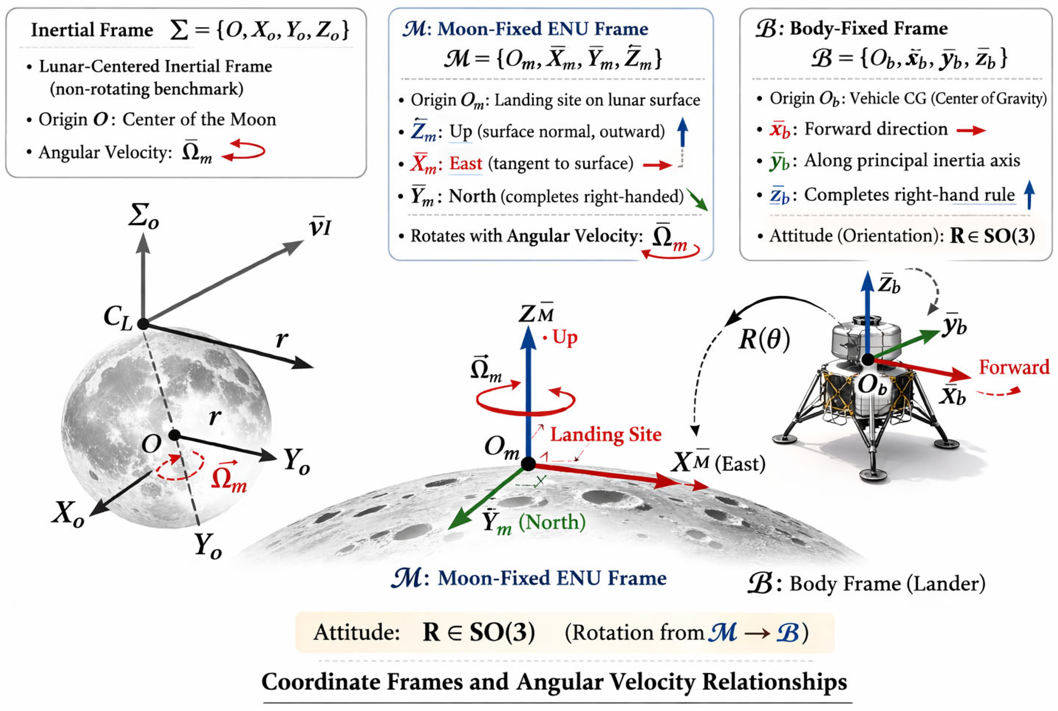
The coordinate frames employed in this manuscript are illustrated in Figure 1. To clearly describe the translational and rotational motion of the vehicle, we define the following right-handed Cartesian coordinate systems.

The inertial frame, denoted as Σ = {O, X_o, Y_o, Z_o}, is a lunar-centered inertial frame. Its origin O is located at the center of the lunar surface. This frame serves as the non-rotating benchmark against the Moon, characterized by the angular velocity Ω_m.

The Moon-fixed local frame, denoted as M = {O_m, X_m, Y_m, Z_m}, is crucial for defining the landing constraints and is the primary frame for trajectory planning located at the designated landing site on the lunar surface. The Z_m-axis is aligned with the local surface normal, pointing outward (Up direction). The X_m-axis points toward the local East direction, tangent to the lunar surface. The Y_m-axis completes the right-handed system, pointing toward the local North direction, as shown in Figure 1. This frame is rigidly attached to the lunar surface and therefore rotates with an angular velocity Ω_m relative to the inertial frame.

The body-fixed frame, denoted as B = {O_b, x_b, y_b, z_b}, is attached to the vehicle to describe its attitude and angular velocity. Its origin O_b is located at the vehicle’s center of gravity. The axes are defined based on the vehicle’s principal axes of inertia: The y_b-axis is aligned with the principal axis of inertia. The x_b-axis points outward along the vehicle’s forward direction. The z_b-axis follows the right-hand rule to complete the orthogonal triad. The attitude of the lander, i.e., the orientation of the body-fixed frame B with respect to the Moon-fixed frame M, is represented by the rotation matrix R ∈ SO(3), as depicted in Figure 1.

$$m\left(t\right)={\displaystyle \frac{{‖\mathbf{T}\left(t\right)‖}^2}{I_{sp}{g}_e}}$$

(1)

$${\dot{\mathbf{r}}}_i\left(t\right)={\mathbf{v}}_i\left(t\right)$$

(2)

$${\dot{\mathbf{v}}}_i\left(t\right)={\displaystyle \frac{{\mathbf{T}}_i}{m\left(t\right)}}+\mathbf{g}\left({\mathbf{r}}_i\right)$$

(3)

in which

$$\mathbf{g}\left(\mathbf{r}\right)=-{\displaystyle \frac{{\mu }_m}{{‖\mathbf{r}‖}^3}}{\mathbf{r}}_i$$

(4)

where ${\mu }_m=GM$ denotes the lunar gravitational parameter, G is the universal gravitational constant, M is the mass of the Moon, and r_i represents the position vector of the spacecraft in the inertial reference frame.

m is the mass of the vehicle, r(t) is the inertial position, v(t) is the inertial velocity, and T(t) is the thrust of the main engine of the vehicle:

$${\mathbf{T}}_i=C_b^i{\mathbf{T}}_b$$

(5)

where $C_b^m$ is the rotation matrix from the body frame B to the inertial frame Σ. I_sp is the specific impulse of the propellants, and g_e = 9.8 m/s² is the gravity of Earth.

Since the translational states (position and velocity) are propagated in the inertial frame Σ while the attitude is expressed in M, the kinematic relationship between the two frames must be explicitly defined. The frame M rotates with respect to Σ at a constant angular velocity.

Let r_i be the position vector in the inertial frame and r_m be the position vector in the Moon-fixed frame. The transformation between them is given by

$${\mathbf{r}}_i=C_m^i{\mathbf{r}}_m$$

(6)

where $C_m^i$ in SO(3) is the rotation matrix from the Moon-fixed frame M to the inertial frame Σ, satisfying the following differential equation:

$${\dot{C}}_m^i=C_m^i{\left[{\mathbf{\Omega }}_m\right]}_{\times }$$

(7)

Here, ${\left[{\mathbf{\Omega }}_m\right]}_{\times }$ is the skew-symmetric matrix (also known as the cross-product matrix) constructed from the angular velocity vector ${\mathbf{\Omega }}_m$, defined as

$$\begin{array}{c}{\left[{\mathbf{\Omega }}_m\right]}_{\times }=\left[\begin{array}{ccc}0& -{\Omega }_z& {\Omega }_y\\ {\Omega }_z& 0& -{\Omega }_x\\ -{\Omega }_y& {\Omega }_x& 0\end{array}\right]\\ {\mathbf{\Omega }}_m={\left[\begin{array}{ccc}{\Omega }_x& {\Omega }_y& {\Omega }_z\end{array}\right]}^T\end{array}$$

Differentiating the position relationship yields the relationship between the inertial velocity v_i and the Moon-fixed velocity v_m:

$${\mathbf{v}}_i={\dot{\mathbf{r}}}_i=C_m^i{\dot{\mathbf{r}}}_m+{\dot{C}}_m^i{\mathbf{r}}_m=C_m^i\left({\mathbf{v}}_m+{\mathbf{\Omega }}_m\times {\mathbf{r}}_m\right)$$

(8)

That is,

$${\mathbf{v}}_i=C_m^i\left({\mathbf{v}}_m+{\mathbf{\Omega }}_m\times {\mathbf{r}}_m\right)$$

(9)

Differentiating the velocity relationship once more yields the expression for the inertial acceleration:

$${\mathbf{a}}_i={\dot{\mathbf{v}}}_i=C_m^i\left[{\mathbf{a}}_m+2{\mathbf{\Omega }}_m\times {\mathbf{v}}_m+{\mathbf{\Omega }}_m\times \left({\mathbf{\Omega }}_m\times {\mathbf{r}}_m\right)+{\dot{\mathbf{\Omega }}}_m\times {\mathbf{r}}_m\right]$$

(10)

Since the lunar angular velocity is constant, ${\dot{\mathbf{\Omega }}}_m$ = 0, the above expression simplifies to

$${\mathbf{a}}_i=C_m^i\left[{\mathbf{a}}_m+2{\mathbf{\Omega }}_m\times {\mathbf{v}}_m+{\mathbf{\Omega }}_m\times \left({\mathbf{\Omega }}_m\times {\mathbf{r}}_m\right)\right]$$

(11)

where $a_{cen}=‖{\mathbf{\Omega }}_m\times \left({\mathbf{\Omega }}_m\times {\mathbf{r}}_m\right)‖$ is the Coriolis acceleration, and $a_{cor}=‖2{\mathbf{\Omega }}_m\times {\mathbf{v}}_m‖$ is the centripetal acceleration.

If the vehicle dynamics are expressed in the Moon-fixed frame M, the dynamic equation in the inertial frame ${\mathbf{a}}_i={\mathbf{T}}_i/m+{\mathbf{g}}_i$ must be substituted into the acceleration transformation relationship, yielding

$${\mathbf{a}}_m+2{\mathbf{\Omega }}_m\times {\mathbf{v}}_m+{\mathbf{\Omega }}_m\times \left({\mathbf{\Omega }}_m\times {\mathbf{r}}_m\right)={\mathbf{g}}_m\left({\mathbf{r}}_m\right)+{\mathbf{T}}_m/m$$

(12)

Rearranging gives the complete dynamic equations in the Moon-fixed frame:

$${\mathbf{a}}_m={\mathbf{g}}_m{\mathbf{r}}_m+{\mathbf{T}}_m/m-2{\mathbf{\Omega }}_m\times {\mathbf{v}}_m-{\mathbf{\Omega }}_m\times \left({\mathbf{\Omega }}_m\times {\mathbf{r}}_m\right)$$

(13)

where ${\mathbf{T}}_m=\mathbf{R}{\mathbf{T}}_b$ is the representation of the body frame thrust ${\mathbf{T}}_b$ in the Moon-fixed frame, and R is the rotation matrix from the body frame to the Moon-fixed frame.

For lunar powered descent phases, the total duration is typically less than 600 s. Under these conditions, the engineering validity of neglecting the Coriolis and centripetal acceleration terms can be assessed. For the Moon, $‖{\mathbf{\Omega }}_m‖\approx 2.66\times {10}^{-6} \mathrm{rad}/\mathrm{s}$.

$‖a_{cen}‖$ is on the order of $9\times {10}^{-3}{\mathrm{m}/\mathrm{s}}^2$, so the Coriolis term contributes at most a relative level of O(10⁻³)–O(10⁻²). Over the landing phase, the velocity increment caused by Coriolis remains only a few m/s, which is within the typical dispersions/margins of powered descent guidance and can be treated as a small modeling error. The centrifugal term $‖a_{cor}‖$ is even smaller and remains ≪10⁻⁴ m/s².

2.2. Mathematical Foundation of the Normalized Finite Rotation Angle Parametrization

To establish a rigorous geometric and computational foundation for the proposed attitude representation, this section reformulates the finite rotation angle (FRA) parametrization as the exponential coordinate representation on the Lie group SO(3). Explicit mappings to quaternion and Modified Rodrigues Parameters (MRP) are provided, together with the singularity analysis, numerical stabilization strategies, and consistent angular velocity relations required for six-degree-of-freedom dynamics.

2.2.1. FRA as Exponential Coordinates on SO(3)

According to Euler’s rotation theorem, any rigid-body orientation can be represented as a single rotation of angle θ ∈ ℝ about a fixed unit axis n ∈ ℝ³, where $‖\mathrm{n}‖ = 1$.

The FRA representation consolidates this into a minimal three-dimensional vector:

$$\theta =\theta \mathbf{n}, \theta =‖\mathit{\theta }‖$$

The vector θ ∈ ℝ³ is an element of the Lie algebra through its associated skew-symmetric matrix:

$${\mathit{\theta }}^{\wedge }=\left[\begin{array}{ccc}0& -{\theta }_3& {\theta }_2\\ {\theta }_3& 0& -{\theta }_1\\ -{\theta }_2& {\theta }_1& 0\end{array}\right]$$

The corresponding rotation matrix R ∈ SO(3), transforming vectors from the body-fixed frame to the Moon-fixed frame, is obtained through an exponential map:

$$\mathbf{R}=\exp \left({\mathit{\theta }}^{\wedge }\right)$$

(14)

Using Rodrigues’ formula, the exponential map admits the explicit closed form:

$$\mathbf{R}\left(\mathbf{\theta }\right)=\mathbf{I}+{\displaystyle \frac{\sin \theta }{\theta }}{\mathit{\theta }}^{\wedge }+{\displaystyle \frac{\left(1-\cos \theta \right)}{\theta }}{\left({\mathit{\theta }}^{\wedge }\right)}^2$$

(15)

This establishes FRA as the exponential coordinate representation of rotations on SO(3).

2.2.2. Geometric Interpretation, Uniqueness, and the Geodesic Property

The exponential map exp: $\mathfrak{s}\mathfrak{o}\left(3\right)\to SO\left(3\right)$ is surjective but not injective. Multiple rotation vectors correspond to the same rotation matrix:

$$\theta \sim \theta +2k\pi \mathbf{n}$$

To ensure a unique representation, the magnitude is restricted to the principal branch of the logarithm map on SO(3):

$$\theta \in \left(-\pi ,\pi \right]$$

This restriction corresponds to selecting the principal value of the rotation angle and ensures a one-to-one mapping between the rotation vector and the rotation matrix, except at the boundary.

The exponential map is a local diffeomorphism for θ ≠ π. The only true singular configuration in this representation occurs at θ = π, where the rotation axis becomes non-unique and the tangent operator loses invertibility. This is a fundamental property of any three-dimensional parametrization of rotation. Importantly, for θ = 2 kπ, the map is not singular; it is simply not injective, as it maps distinct vectors to the same rotation matrix ($\mathbf{R}=\mathbf{I}$). The non-injectivity is resolved using the principal value restriction.

Furthermore, under the canonical bi-invariant metric on SO(3), the geodesic curves are given by

$$\mathbf{R}\left(t\right)=\exp \left(t{\mathit{\theta }}_f^{\wedge }\right), t\in \left[0,1\right]$$

(16)

Thus, the linear interpolation in the FRA space, $\mathit{\theta }\left(t\right)=t{\mathit{\theta }}_f$, corresponds exactly to geodesic motion in SO(3). This geometric property guarantees that trajectory planning using FRA preserves minimal rotational paths, consistent with methods such SLERP (spherical linear interpolation) for quaternions, but within a minimal, unconstrained vector space.

Therefore, the polynomial interpolation defined later in Equations (34)–(36) for the reference trajectory is consistent with this geodesic property, ensuring that the attitude motion follows a minimal rotational path.

2.2.3. Mapping to Standard Attitude Representations

A unit quaternion $\mathbf{q}=\left(q_0,\mathbf{q}\right)$ satisfies $q_0^2+{‖\mathbf{q}‖}^2=1$. Given FRA θ, the equivalent quaternion is

$$q_0=\cos \left({\displaystyle \frac{\theta }{2}}\right), \mathbf{q}={\displaystyle \frac{\mathit{\theta }}{\theta }}\sin \left({\displaystyle \frac{\theta }{2}}\right)$$

(17)

The FRA vector can be recovered from a quaternion as

$$\mathit{\theta }=2\arccos \left(q_0\right){\displaystyle \frac{\mathbf{q}}{‖\mathbf{q}‖}}\left(‖\mathbf{q}‖>0\right)$$

(18)

Apparently, the FRA does not require a unit-norm constraint, thus eliminating the need for normalization or solving differential-algebraic equations (DAEs) within an optimization framework.

MRP is defined as $\mathit{\sigma }=\tan \left({\displaystyle \frac{\theta }{4}}\right)\mathbf{n}$. The mapping to FRA is

$$\mathit{\theta }=4\arctan \left(‖\mathit{\sigma }‖\right){\displaystyle \frac{\mathit{\sigma }}{‖\mathit{\sigma }‖}}$$

(19)

MRP exhibits a singularity at θ = ±2π, whereas FRA’s principal value singularity occurs at θ = π. FRA therefore avoids the shadow set switching strategies required by MRP to cover the full rotation space, simplifying the implementation in iterative algorithms.

2.2.4. Angular Velocity and Acceleration Mapping

For trajectory optimization, it is necessary to establish a consistent mapping between the FRA parameters and the physically meaningful angular velocity and angular acceleration. Following the standard convention in rigid-body dynamics [33], we define the rotation matrix. Differentiating the exponential map yields

$$\dot{\mathbf{R}}=\mathbf{R}{\mathit{\omega }}_b^{\wedge }$$

(20)

where ${\mathit{\omega }}_b^{\wedge }$ is the skew-symmetric matrix associated with the body frame angular velocity ω_b ∈ ℝ³.

$${\mathit{\omega }}_b^{\wedge }={\mathbf{R}}^T\dot{\mathbf{R}}$$

(21)

which expresses the angular velocity in the body frame.

The exact kinematic relation between the FRA rates and the body frame angular velocity is given by

$${\mathbf{\omega }}_b=\mathbf{T}\left(\theta \right)\dot{\mathit{\theta }}$$

(22)

where T(θ) is the left Jacobian (or tangent operator) that maps the time derivatives of the rotation vector to the physical angular velocity. This operator is expressed explicitly as

$$\mathbf{T}\left(\mathbf{\theta }\right)=\mathbf{I}-{\displaystyle \frac{1-\cos \theta }{{\theta }^2}}{\mathit{\theta }}^{\wedge }+{\displaystyle \frac{\left(\theta -\sin \theta \right)}{{\theta }^3}}{\left({\mathit{\theta }}^{\wedge }\right)}^2$$

(23)

The body frame angular acceleration follows as the time derivative of Equation (22):

$${\dot{\mathbf{\omega }}}_b=\mathbf{T}\left(\theta \right)\ddot{\mathit{\theta }}+\dot{\mathbf{T}}\left(\theta ,\dot{\mathit{\theta }}\right)\dot{\mathit{\theta }}$$

(24)

These relations provide an exact, nonlinear mapping between the generalized FRA coordinates $\left(\mathit{\theta },\dot{\mathit{\theta }},\ddot{\mathit{\theta }}\right)$ and the physical rotational states $\left({\mathit{\omega }}_b,{\dot{\mathit{\omega }}}_b\right)$ expressed in the body-fixed frame B.

For completeness, the transformation between the body frame and inertial frame angular velocities is given by the rotation matrix.

2.2.5. Numerical Stabilization Strategies

For θ→0, the direct evaluation of the trigonometric ratios in Equations (15) and (23) leads to numerical cancelation due to the 0/0 indeterminacy. To ensure numerical robustness, we employ Taylor series expansions:

$${\displaystyle \frac{\sin \theta }{\theta }}=1-{\displaystyle \frac{{\theta }^2}{6}}+{\displaystyle \frac{{\theta }^4}{120}}+\mathcal{O}\left({\theta }^6\right)$$

(25)

$${\displaystyle \frac{1-\cos \theta }{\theta }}={\displaystyle \frac{1}{2}}-{\displaystyle \frac{{\theta }^2}{24}}+{\displaystyle \frac{{\theta }^4}{720}}+\mathcal{O}\left({\theta }^6\right)$$

(26)

$${\displaystyle \frac{\theta -\cos \theta }{{\theta }^3}}={\displaystyle \frac{1}{6}}-{\displaystyle \frac{{\theta }^2}{5!}}+{\displaystyle \frac{{\theta }^4}{7!}}+\mathcal{O}\left({\theta }^6\right)$$

(27)

Retaining four to five terms in these series ensures a machine-level precision for all subsequent computations, effectively removing the removable singularity at θ = 0.

2.2.6. Computational Advantages for Convex Optimization

Compared to other attitude representations commonly used in trajectory optimization, the normalized FRA formulation offers several distinct advantages.

These characteristics make FRA particularly suitable for trajectory optimization frameworks that rely on repeated linearization and efficient numerical solution, as demonstrated in the numerical examples in Section 4.

To define an achievable attitude curve for the reference landing trajectory, it is necessary to normalize the angles to simplify the connections of skew to the rotations and to avoid the singularity of specific angles. Here, we utilize the method from reference [39] to nullify the initial FRAs.

For the description of the attitude motion along the reference trajectory, the initial orientation of the FRAs must be nullified. Considering the description of the finite rotation angle from ${\mathit{\theta }}_0$ to ${\mathit{\theta }}_f$ over time t₀ to t_f, the initial and final CTM can be expressed as R₀ and R_f, respectively. The dimensionless time variable can be written as

$$\mathit{\kappa }={\displaystyle \frac{t-t_0}{t_f-t_0}}$$

(28)

And the smooth attitude motion description function f(κ) can be defined as

$$\begin{array}{l}\mathbf{R}\left(\mathit{\kappa }\right)={\mathbf{R}}_0+f\left(\mathit{\kappa }\right)\left({\mathbf{R}}_f-{\mathbf{R}}_0\right)\\ \mathit{\theta }\left(\mathit{\kappa }\right)={\mathit{\theta }}_0+f\left(\mathit{\kappa }\right)\left({\mathit{\theta }}_f-{\mathit{\theta }}_0\right)\end{array}$$

(29)

The linear interpolation can be achieved by using f(κ) = κ, which represents constant angular velocity. However, the linear interpolation using f(κ) cannot be represented by $\mathbf{R}\left(\mathit{\kappa }\right)$, as the matrix is not orthogonal. Furthermore, the angular motion cannot be described accurately with a constant angular velocity. For that purpose, we assume that the attitude motion can be described by $\widehat{\mathbf{R}}\left(\mathit{\kappa }\right)$:

$$\mathbf{R}\left(\mathit{\theta }\left(\mathit{\kappa }\right)\right)=\mathbf{R}\left(\widehat{\mathit{\theta }}\left(\mathit{\kappa }\right)\right)\mathbf{R}\left({\mathit{\theta }}_0\right)$$

(30)

$$\mathbf{R}\left({\mathit{\theta }}_f\right)=\mathbf{R}\left({\widehat{\mathit{\theta }}}_f\right)\mathbf{R}\left({\mathit{\theta }}_0\right)$$

(31)

where ${\widehat{\mathit{\theta }}}_f=\widehat{\mathit{\theta }}\left(1\right)$ at the end time t_f. The angular velocity can be described by $\widehat{\mathit{\theta }}\left(\mathit{\kappa }\right)=\mathit{\kappa }{\widehat{\mathit{\theta }}}_f$. And the angular acceleration along the trajectory can be clearly identified by the function of κ.

To normalize the FRAs, we transform $\mathbf{R}\left({\mathit{\theta }}_f\right)$ as follows:

$$\widehat{\mathbf{R}}\left({\mathit{\theta }}_f\right)={\mathbf{R}}^T\left({\mathit{\theta }}_0\right)\mathbf{R}\left({\mathit{\theta }}_f\right)$$

(32)

After that, ${\widehat{\mathit{\theta }}}_f$ can be defined by $\widehat{\mathbf{R}}\left({\widehat{\mathit{\theta }}}_f\right)$.

Then,

$$\widehat{\mathit{\theta }}\left(\mathit{\kappa }\right)=\mathit{\kappa }{\widehat{\mathit{\theta }}}_f$$

(33)

We can describe the angular velocity and the attitude accurately. Finally,

$$\mathbf{R}\left(\mathit{\theta }\left(\mathit{\kappa }\right)\right)=\mathbf{R}\left({\mathit{\theta }}_0\right)\mathbf{R}\left(\widehat{\mathit{\theta }}\left(\mathit{\kappa }\right)\right)$$

We can recover the original $\mathit{\theta }\left(\mathit{\kappa }\right)$. Because the initial FRAs are nullified by ${\widehat{\mathit{\theta }}}_0=\mathbf{0}$, the rotational description can be determined only by ${\widehat{\mathit{\theta }}}_f$.

In this manuscript, we introduce a polynomial interpolation method to suit the angular velocities and angles for the reference trajectory. By applying the high-order polynomial function of a dimensionless time variable to the angles and angular velocities, the corresponding control variables within the reference trajectory are derived by the correct kinematic relationship. We assume that the attitude motion can be described using the invalid time variable κ as follows:

$$\widehat{\mathbf{\theta }}\left(\mathit{\kappa }\right)=\lambda \left(\mathit{\kappa }\right){\widehat{\mathbf{\theta }}}_f$$

(34)

$$\lambda \left(\mathit{\kappa }\right)=z_0{\mathit{\kappa }}^2-z_1{\mathit{\kappa }}^3+z_2{\mathit{\kappa }}^4+\cdots$$

(35)

The coefficients z_j (j = 0,1,2) can be decided by the initial and final conditions of the attitude, angular velocity, and angular acceleration:

$${\displaystyle \frac{d\widehat{\mathit{\theta }}}{d\mathit{\kappa }}}={\displaystyle \frac{1}{\Delta t}}{\displaystyle \frac{d\lambda \left(\mathit{\kappa }\right)}{d\mathit{\kappa }}}{\widehat{\mathit{\theta }}}_f$$

(36)

$${\displaystyle \frac{d^2\widehat{\mathit{\theta }}}{d{\mathit{\kappa }}^2}}={\displaystyle \frac{1}{\Delta t^2}}{\displaystyle \frac{d^2\lambda \left(\mathit{\kappa }\right)}{d{\mathit{\kappa }}^2}}{\widehat{\mathit{\theta }}}_f$$

(37)

2.3. Constraints

The boundary conditions of the proposed guidance strategy are straightforward; the initial and desired terminal conditions of the vehicle’s state vector are treated as hard constraints. The translational dynamics and attitude dynamics, can be expressed as follows:

$$m\left(t_0\right)=m_0 \mathbf{r}\left(t_0\right)=r_0 \mathbf{v}\left(t_0\right)=v_0 \mathbf{\theta }\left(t_0\right)={\mathbf{\theta }}_0 \mathbf{\omega }\left(t_0\right)={\mathbf{\omega }}_0$$

The terminal state boundary constraints are as follows:

$$\mathbf{r}\left(t_f\right)=r_f \mathbf{v}\left(t_f\right)=v_f \mathbf{\theta }\left(t_f\right)={\left[\begin{array}{ccc}0& \frac{\pi }{2}& 0\end{array}\right]}^{\mathrm{T}} \mathbf{\omega }\left(t_f\right)=\mathbf{0}$$

The vehicle is positioned upright to meet the requirement of achieving a vertical landing.

Next, the manuscript examines the state constraints that must be satisfied along the trajectory’s optimization. The total amount of fuel determines the duration of the vehicle’s propulsion system. Throughout the whole landing phase, the fuel consumption is constrained by inequalities:

$$m\left(t_f\right)\ge m_{d\mathbf{r}y}$$

(38)

In this manuscript, the vehicle is in the final stage of powered descent. By imposing restrictions on the vehicle’s angular body rates, excessive rotations are mitigated, enabling smoother descent maneuvers, particularly in the context of the vertical landing requirement:

$$‖{\mathbf{\omega }}_B\left(t\right)‖\le {\omega }_{\max }$$

(39)

The main engine operates within a specific range of thrust values, denoted as [T_min, T_max]. Additionally, it is necessary to consider the multiple-ignition assumption, meaning that the engine is not maintained in a continuous-thrust maneuver during the powered descent phase. Furthermore, the thrust vector control system of the engine is limited by the angular deflection capacity due to its mechanical structure. By incorporating these constraints, the trajectory optimization ensures that the commanded thrust remains within the permissible range and accounts for the operational limitations of the engine’s thrust vector control system:

$$0<T_{\min }\le {‖\mathbf{T}\left(t\right)‖}_2\le T_{\max }$$

(40)

$$\cos {\delta }_{\max }{‖\mathbf{T}\left(t\right)‖}_2\le z_b^{\mathrm{T}}\mathbf{T}\left(t\right)$$

(41)

where we assume that δ_max ≤ 90°, and ${\mathbf{z}}_b$ is a SO(3) group.

In the trajectory optimization, the upper thrust bound naturally forms a convex constraint. However, the lower bound introduces a non-convex constraint, which is a problem for the successive convexification problem. Alternative formulations demonstrate that this non-convexity can be effectively transformed into a lossless convex constraint. Therefore, in the problem addressed here, we employ linearization to transform the non-convexity from the discretization step, which will be detailed in Section 3.2. This approach allows us to address the non-convex nature of the lower thrust bound and effectively incorporate it into the trajectory optimization algorithm.

Finally, the cost function of the continuous time optimal trajectory programming problem is formulated as follows:

$$\min -m\left(t_f\right)$$

(42)

Fuel optimization is attained under the vehicle’s dynamic and kinematic framework, given that the boundary and control constraints are satisfied.

3. Convex Formulation

The above problem is defined as a free final time problem with non-convex constraints and variables. To solve the original problem, we transform it into a series of convex subproblems with a fixed final time through lossless convexification. Then, the trajectory optimization problem can be solved optimally using the interior-point method. In this manuscript, we focus on the initialization method, using the fast iterative gradient method to modify the initial guess of the reference trajectory and converge to the optimal solution rapidly.

3.1. Initialization Setup

Firstly, we define the state vector x(t) ∈ ℝ^13×1 and control vector u(t) ∈ ℝ^3×1:

$$\mathbf{x}\left(t\right)={\left[\begin{array}{ccccc}m\left(t\right)& \mathbf{r}\left(t\right)& \mathbf{v}\left(t\right)& \mathbf{\theta }\left(t\right)& \mathbf{\omega }\left(t\right)\end{array}\right]}^{\mathrm{T}}$$

$$\mathbf{u}\left(t\right)=\mathbf{T}\left(t\right)$$

Accordingly, the nonlinear dynamics can be expressed as follows:

$$f\left(\mathbf{x}\left(t\right),\mathbf{u}\left(t\right)\right)={\displaystyle \frac{d}{dt}}\mathbf{x}\left(t\right)={\left[\begin{array}{ccccc}\dot{m}\left(t\right)& \dot{\mathbf{r}}\left(t\right)& \dot{\mathbf{v}}\left(t\right)& \dot{\mathbf{\theta }}\left(t\right)& \dot{\mathbf{\omega }}\left(t\right)\end{array}\right]}^{\mathrm{T}}$$

To address the trajectory planning problem with a free final time objective, we introduce the concept of time dilation, which involves evaluating the system dynamics using a normalized trajectory time variable, denoted as τ. Regardless of the optimization resolution, the terminal value of τ is always τ = 1, representing the final time.

Additionally, we introduce the variable η as a scaling factor to represent the non-dimensionalized final time in the convex subproblem. This allows us to account for various scaling factors, such as time, which influence trajectory generation. By adjusting these factors through η, we can accurately model and analyze the system’s behavior and performance:

$$\eta \triangleq {\left(\frac{d\tau }{dt}\right)}^{-1}$$

(43)

By introducing a normalized time variable, this transformation enables the final time to be treated as an optimization variable, offering the flexibility to determine the optimal trajectory duration:

$$f\left(\mathbf{x}\left(t\right),\mathbf{u}\left(t\right)\right)={\displaystyle \frac{d}{dt}}\mathbf{x}\left(t\right)={\displaystyle \frac{d\tau }{dt}}{\displaystyle \frac{d}{d\tau }}\mathbf{x}\left(t\right)={\displaystyle \frac{1}{\eta }}{\displaystyle \frac{d}{d\tau }}\mathbf{x}\left(t\right)$$

(44)

Scaling Matrices

In practice, numerical issues associated with sensitivity, machine precision, and the choice of termination criteria can arise in a numerical solver when these magnitudes are highly different. We use the standard remedy of applying affine variable transformations:

$${\mathit{x}}_i=P_x{\widehat{\mathit{x}}}_i+{\mathit{p}}_x$$

(45)

$${\mathit{u}}_i=P_u{\widehat{\mathit{u}}}_i+{\mathit{p}}_u$$

(46)

$$z_i=P_z\widehat{z}$$

(47)

The scaling terms are chosen such that the components of the scaled state ${\widehat{\mathit{x}}}_i$, the scaled input ${\widehat{\mathit{u}}}_i$, and the scaled dilation factor $z_i$ have the maximum magnitude of roughly unity across all iterations.

3.2. Linearization of the Nonlinear Dynamic Model

By employing a first-order Taylor series approximation, the nonlinear dynamic problem is transformed into a time-varying linear system of equations that will be utilized in our algorithm to simplify the calculations and enable efficient computation. The reference trajectory obtained through the initial guess method is expressed as $\left(\widehat{\mathbf{x}},\widehat{\mathbf{u}},\widehat{\eta }\right)$; the time-varying linear equations over the interval [0, 1] are calculated. This approach enables efficient trajectory planning while ensuring the desired accuracy:

$${\mathbf{x}}^{\prime }\left(\tau \right)=\eta \Sigma \left(\tau \right)+A\left(\tau \right)\mathbf{x}+B\left(\tau \right)\mathbf{u}+\mathbf{z}\left(\tau \right)$$

(48)

This expression is simplified by breaking the Taylor expansion into matrix subcomponents:

$$A\left(\tau \right)\triangleq \widehat{\eta }{\left.{\displaystyle \frac{\partial \mathbf{f}}{\partial \mathbf{x}}}\right|}_{\widehat{\mathbf{x}},\widehat{\mathbf{u}}}$$

(49)

$$B\left(\tau \right)\triangleq {\left.\widehat{\eta }{\displaystyle \frac{\partial \mathbf{f}}{\partial \mathbf{u}}}\right|}_{\widehat{\mathbf{x}},\widehat{\mathbf{u}}}$$

(50)

$$\Sigma \left(\tau \right)\triangleq \mathbf{f}\left(\widehat{\mathbf{x}}\left(\tau \right),\widehat{\mathbf{u}}\left(\tau \right)\right)$$

(51)

$$\mathbf{z}\left(\tau \right)\triangleq -A\left(\tau \right)\widehat{\mathbf{x}}-B\left(\tau \right)\widehat{\mathbf{u}}$$

(52)

Then, we address the remaining factors contributing to non-convexity and the non-zero lower bound of the thrust on the main engine. To handle this, we introduce a ${\mathbb{R}}^3\to \mathbb{R}$ mapping function denoted as $g\left(\mathbf{u}\left(\tau \right)\right)=T_{\min }-{‖\mathbf{u}\left(\tau \right)‖}_2\le 0$, which represents the minimum allowable thrust. By utilizing a first-order Taylor series linear approximation, we can derive the convexified constraint formulation:

$$g\left(\mathbf{u}\left(\tau \right)\right)=T_{\min }-\Xi \left(\tau \right)\mathbf{u}\left(\tau \right)$$

(53)

This leads us to the linear, convexified constraints, which entail the use of the linearization path value $\widehat{\mathbf{u}}$.

3.3. Discretization Scheme

Through discretization, the continuous-time dynamics, state, and control constraints are transformed into finite-dimensional second-order problems. This allows us to apply numerical methods and algorithms to efficiently solve the optimal trajectory while satisfying the specified conditions and constraints. By normalizing the time within the interval [0, 1], it is discretized into k uniformly spaced points, denoted as τ. Consequently, the discrete dynamics at each time point τ_k are represented as

$${\mathbf{x}}_{k+1}=F_k{\mathbf{x}}_k+G_k^{-}{\mathbf{u}}_k+G_k^{+}{\mathbf{u}}_{k+1}+{\overline{z}}_k+{\overline{\Sigma }}_k\eta$$

(54)

where $F_k$, $G_k^{-}$, $G_k^{-}$, ${\overline{z}}_k$, and ${\overline{\Sigma }}_k$ represent the integrations of the state transformation matrix.

3.4. Initial Solution Guess

This manuscript aims to develop an efficient initial solution guessing method to provide reasonable reference values for solving convex subproblems iteratively and reducing the number of iterations. To achieve this, we draw on the principles of the iterative gradient descent algorithm. A feasible way to solve the convex problem is by using the matrix vector multiplication involving each iteration, followed by a shrinkage step to effectively decrease the computational effort. This method finds the minimum of the convex function in a feasible set through projection.

3.4.1. Global Dynamics Matrix Assembly

Consider discrete time nodes indexed by k = 0, 1, …, K. The state at each node is defined as

$$x_k=\left[m_k;r_k;v_k;{\theta }_k;{\omega }_k\right]\in {\mathbb{R}}^{n_x}$$

(55)

where $m_k$ ∈ ℝ, r_k, v_k, ω_k ∈ ℝ³, and θ_k ∈ ℝ^nθ. Consequently, the dimension of the state vector is

$$n_{\mathrm{x}} = 1 + 3 + 3 + \mathrm{n}\theta + 3 = 10 + n_{\theta }$$

The stacked trajectory vector is constructed by concatenating the states at all nodes:

$$x={\left[x_0^T;x_1^T;\dots ;x_K^T\right]}^T\in {\mathbb{R}}^{\left(K+1\right)n_x}$$

(56)

To explicitly construct the global dynamics residual matrix A and vector b, we begin with the discretized dynamics. The nonlinear continuous-time dynamics are discretized using a fixed time step Δt as follows:

$$x_{k+1}=x_k+\Delta t\cdot f\left(x_k,u_k\right)$$

(57)

Linearizing the dynamics around a reference trajectory yields

$$f\left(x,u\right)\approx A_{k}x+B_{k}u+c_k$$

(58)

where $A_k\in {\mathbb{R}}^{n_x\times n_x}$, $B_k\in {\mathbb{R}}^{n_x\times n_u}$, and $c_k\in {\mathbb{R}}^{n_x}$ (we assume B_k is the full rank for all k, ensuring the well-posedness of the control problem). Substituting this linearization into the discretized dynamics gives the local affine constraint:

$$x_{k+1}-x_k-\Delta t\cdot A_k{x}_k=\Delta t\cdot B_k{u}_k+\Delta t\cdot c_k$$

(59)

Rearranging the terms, this can be expressed as a linear equality constraint in the global state vector. The global residual matrix $A_k\in {\mathbb{R}}^{\left(K+1\right)n_x\times \left(K+1\right)n_x}$ and $B_k\in {\mathbb{R}}^{\left(K+1\right)n_x}$ are assembled by embedding each local linearized relation into the global coordinate system, ensuring that the condition Ax − b = 0 enforces the discretized dynamics across all nodes.

The assembly follows the sparsity pattern induced by temporal discretization, yielding a block-structured matrix of the form

$$A=\left[\begin{array}{ccccc}-I& I& 0& \dots & 0\\ 0& -I& I& \dots & 0\\ ⋮& & \ddots & \ddots & ⋮\\ 0& \dots & 0& -I& I\end{array}\right]-\Delta t\left[\begin{array}{cccc}{A}_0& 0& \dots & 0\\ 0& A_0& \dots & 0\\ ⋮& ⋮& \ddots & ⋮\\ 0& 0& \dots & A_0\\ 0& 0& \dots & 0\end{array}\right]$$

(60)

with the corresponding vector b constructed from the terms ΔtB_ku_k + Δtc_k.

To promote smoothness in the mass, position, and velocity profiles, we first define a component selection matrix that extracts these components from the full state at a single node:

$$S_x=\left[\begin{array}{ccccc}{I}_1& 0& 0& 0& 0\end{array};\begin{array}{ccccc}0& I_3& 0& 0& 0\end{array};\begin{array}{ccccc}0& 0& I_3& 0& 0\end{array}\right]\in {\mathbb{R}}^{7\times n_x}$$

which maps $x_k=\left[m_k;r_k;v_k;{\theta }_k;{\omega }_k\right]$ to $S_x{x}_k=\left[m_k;r_k;v_k\right]\in {\mathbb{R}}^7$.

Extending this selection to the entire trajectory via a Kronecker product yields the global selection matrix:

$$S=I_{K+1}\otimes S_x\in {\mathbb{R}}^{\left(K+1\right)n_x\times \left(K+1\right)n_x},$$

such that the stacked vector containing only mass, position, and velocity is given by x_s = S_x.

For the second-order difference operator acting on the time dimension, we define $D_{2,\tau }\in {\mathbb{R}}^{\left(K-1\right)\times \left(K+1\right)}$ for a sequence of length K + 1. Its entries are given by

$${\left(D_{2,\tau }\right)}_{i,i}=1, {\left(D_{2,\tau }\right)}_{i,i+1}=-2, {\left(D_{2,\tau }\right)}_{i,i+2}=1$$

for i = 1, …, K − 1 (the indexing can be adjusted to start from 0 without loss of generality).

Extending this operator to the vector dimension (here, the 7-dimensional [m, r, v]) gives

$$D_2=D_{2,\tau }\otimes I_7\in {\mathbb{R}}^{7\left(K-1\right)\times 7\left(K+1\right)}$$

Thus, the second-order smoothing term can be written as

$${‖D_2{x}_s‖}_2^2={‖\left(D_{2,\tau }\otimes I_7\right)I_{K+1}\otimes S_{x}x‖}_2^2$$

For brevity, we combine these operations into a single smoothing operator:

$$\tilde{D}:=D_{2}s={‖\left(D_{2,\tau }\otimes I_7\right)I_{K+1}\otimes S_{x}x‖}_2^2\in {\mathbb{R}}^{7\left(K-1\right)\times \left(K+1\right)n_x},$$

So, the smoothing regularization term is given by ${‖\tilde{D}x‖}_2^2$.

This leads to the following simplified convex subproblem for generating an initial guess:

$$\underset{x\in X}{\min }F\left(x\right)=\frac{1}{2}{‖Ax-b‖}_2^2+\frac{1}{2}{‖\tilde{D}x‖}_2^2$$

(61)

where X ⊂ ℝ^(K+1)nx is a closed convex set formed by state box constraints and boundary conditions. The projection onto this set, denoted by ${\prod }_{\mathcal{X}}\left(\cdot \right)$, remains computationally tractable. The regularization parameter μ > 0 is a numerical parameter that promotes smoothness in the solution; it is not a physically weighted term. Based on empirical studies, μ is typically chosen within the range μ ∈ [10⁻³, 10⁻¹] to balance smoothness with fidelity to the dynamics.

3.4.2. The Fast Gradient Iterative Initial Guess Method

The objective function F(y) is quadratic, with a gradient given by

$$\nabla F\left(y\right)=A^T\left(Ay-b\right)+\lambda {\tilde{D}}^T\tilde{D}y$$

(62)

Let L be an upper bound on the Lipschitz constant of $\nabla F$, i.e., $L\ge ‖A^{T}A+\lambda {\tilde{D}}^T\tilde{D}‖$, which can be estimated via a power iteration. The step size is then set to 1/L.

The iterations proceed as follows for k = 1, 2, …:

$$z_k={\prod }_{\mathcal{X}}\left(y_k-\frac{1}{L}\nabla F\left(y_k\right)\right)$$

(63)

$$t_{k+1}=\frac{1+\sqrt{1+4t_k^2}}{2}$$

(64)

$${\mathbf{y}}_{k+1}={\mathbf{z}}_k+\left(\frac{t_{k-1}}{t_{k+1}}\right)\left({\mathbf{z}}_k-{\mathbf{z}}_f\right)$$

(65)

with t₁ = 1 and an appropriate initialization for y₁ (e.g., a linear interpolation between the specified boundary conditions).

3.4.3. Termination Criterion

1. Oscillation-Based Criterion

To detect whether the iterates have stabilized and oscillations are sufficiently damped, we employ a moving average-based criterion. Let z_k denote the projected gradient iterate at iteration k. Define the moving average of the last m iterates as

$${\overline{\mathbf{z}}}_k=\frac{1}{m}\sum _{j=k-m+1}^k{\mathbf{z}}_j, \mathrm{for} k \ge m$$

(66)

The algorithm terminates when the relative deviation from this moving average falls below a specified tolerance ε_osc > 0:

$$\frac{{‖{\mathbf{z}}_k-{\overline{\mathbf{z}}}_k‖}_2}{\max \left(1,{‖{\overline{\mathbf{z}}}_k‖}_2\right)}\le {\epsilon }_{osc}$$

(67)

This criterion indicates that the iterates have entered a small neighborhood and are no longer making significant progress, regardless of whether the convergence path was monotonic or oscillatory. In this work, we set m = 5 and ε_osc = 10³ for initial guess generation.

2. Maximum Iterations

Additionally, to prevent infinite loops in the case of slow convergence or persistent oscillations, the algorithm terminates when the maximum number of iterations is reached:

$$k\ge k_{max}$$

The maximum iteration count is set to the same value as the outer SCP loop, i.e., k_max = i_max = 20. This ensures consistency between the inner fast gradient iterative initialization and the main successive convexification procedure.

3.4.4. The Algorithm

The solution x∗ obtained from solving this convex problem provides an initial trajectory that lies closer to the local convergence region of the SCP algorithm. Following the local convergence theory for sequential programming methods, a reduction in the initial residual norm directly translates to a decrease in the number of required outer SCP iterations, which is consistent with the trends observed in numerical simulations.

The converged solution x∗: = limk→∞zk for this convex problem is then used as the initial reference trajectory for the main sequential convex programming algorithm, thereby providing a high-quality starting point that enhances convergence performance.

Consequently, the initial iterate lies closer to the local convergence region of SCP. According to classical local convergence analysis of SQP-type methods, the required number of outer iterations decreases as the initial residual norm decreases. This explains the consistent reduction in SCP iterations observed in simulations.

Using this method to compute the initial guess for state parameters, z_k becomes the first reference solution of the sequential convex programming algorithm (Algorithm 1).

Algorithm 1 The fast gradient iterative initial guess method
Input: Matrices A, $\tilde{D}$, vector b, regularization parameter λ, Lipschitz constant L, projection operator ${\prod }_{\mathcal{X}}\left(\cdot \right)$, tolerance ε
Initialize: $y_1=z_0\in \mathcal{X}$ (e.g., linear interpolation between boundary conditions), t1 = 1, k = 1
Repeat:
1:	Compute gradient: $\nabla F\left(y_k\right)=A^T\left(A{y}_k-b\right)+\mu {\tilde{D}}^T\tilde{D}{y}_k$
2:	Projected gradient step. $z_k={\prod }_{\mathcal{X}}\left(y_k-{\displaystyle \frac{1}{L}}\nabla F\left(y_k\right)\right)$
3:	if k ≥ m, then
4	Compute moving average: ${\overline{\mathbf{z}}}_k={\displaystyle \frac{1}{m}}{\displaystyle \sum _{j=k-m+1}^k{\mathbf{z}}_j}$
5:	if ${\displaystyle \frac{{‖{\mathbf{z}}_k-{\overline{\mathbf{z}}}_k‖}_2}{\max \left(1,{‖{\overline{\mathbf{z}}}_k‖}_2\right)}}\le {\epsilon }_{osc}$, then
6:	break
7	end if
8	end if
9	if $k\ge k_{max}$, then
10	break
11	end if
12	Update extrapolation parameter: $t_{k+1}={\displaystyle \frac{1+\sqrt{1+4t_k^2}}{2}}$
13	Extrapolate: ${\mathbf{y}}_{k+1}={\mathbf{z}}_k+\left({\displaystyle \frac{t_{k-1}}{t_{k+1}}}\right)\left({\mathbf{z}}_k-{\mathbf{z}}_f\right)$
14:	k←k + 1
Until	termination criterion satisfied
Output:	Initial reference trajectory ${\mathbf{x}}^0={\mathbf{z}}_k$

3.5. Successive Convexification, Trust Regions and Relaxations

3.5.1. Successive Convexification Framework

An iterative approach involving a sequence of related convex subproblems is employed to solve the optimal trajectory optimization problem. Before reaching the final framework, it is necessary to consider trust regions and dynamic relaxations. Maintaining the boundedness and feasibility of this successive framework during the convergence process requires controlling the divergence of states and inputs from one iteration to the next. Unbounded problems can occur when constraints allow for unbounded costs. To address this, the cost function is augmented with soft trust regions centered on the information from the previous iteration. Let us define these deviations at iteration i as follows:

$$\delta {\mathbf{x}}_k^i\triangleq {\mathbf{x}}_k^i-{\mathbf{x}}_k^{i-1}$$

(68)

$$\delta {\mathbf{u}}_k^i\triangleq {\mathbf{u}}_k^i-{\mathbf{u}}_k^{i-1}$$

(69)

$$\delta {\eta }_k^i\triangleq {\eta }^i-{\eta }^{i-1}$$

(70)

3.5.2. Trust Region Constraints

The constraints after adding the trust regions can be described as follows:

$${‖\delta {\mathbf{x}}_k^i‖}^2+{‖\delta {\mathbf{u}}_k^i‖}^2\le {\overline{\Delta }}_k^i$$

(71)

$${‖\delta {\eta }^i‖}^2\le \Delta {\eta }^i$$

(72)

The trust region radii are incorporated into the cost function as soft penalties:

$$J=J_0+w_{\Delta }^i{‖{\overline{\Delta }}^i‖}^2+w_{\Delta \eta }{‖\Delta {\eta }^i‖}_1$$

(73)

This formulation ensures the boundedness of successive iterates while allowing adaptive step sizes.

To progressively tighten the solution space and accelerate convergence, the trust region penalty weight is updated geometrically:

$$w_{\Delta }^{i+1}={\alpha }_{\Delta }{w}_{\Delta }^i$$

(74)

In this manuscript, ${\alpha }_{\Delta }=1.5\sim 1.7$ is adopted.

3.5.3. Dynamic Relaxation via Virtual Control

As for dynamic relaxation, by adding υ_k to the augmented cost function, the following virtual control history vector will be represented as

$${\upsilon }^i={\left[\begin{array}{ccc}{{\upsilon }_0^i}^{\mathrm{T}}& \dots & {{\upsilon }_{K-2}^i}^{\mathrm{T}}\end{array}\right]}^{\mathrm{T}}$$

And the discrete dynamic equation can be written as follows:

$${\mathbf{x}}_{k+1}^i=F_k^i{\mathbf{x}}_k^i+G_k^{-,i}{\mathbf{u}}_k^i+G_k^{+,i}{\mathbf{u}}_{k+1}^i+{\overline{z}}_k^i+{\overline{\Sigma }}_k\eta +{\upsilon }_k^i$$

(75)

The virtual control relaxes the dynamics temporarily and ensures that the feasible set of the convex subproblem remains non-empty.

An exact ℓ₁-penalty term is appended to the objective function:

$$J=J_0+w_{\Delta }^i{‖{\overline{\Delta }}^i‖}^2+w_{\Delta \eta }{‖\Delta {\eta }^i‖}_1+w_{\upsilon }{‖{\overline{\upsilon }}_k‖}_1$$

(76)

A sufficiently large ${\overline{\upsilon }}_k$→ 0, thereby recovering the original nonlinear dynamics as the algorithm converges.

The following objective function is used:

$$\underset{{\eta }^i}{\min } {\eta }^i+w_{\Delta }^i{‖{\overline{\Delta }}^i‖}_2+w_{\Delta \eta }{‖\Delta {\eta }^i‖}_1+w_{\upsilon }{‖{\overline{\upsilon }}^i‖}_1$$

(77)

If the virtual control norm remains above a prescribed threshold after a fixed number of iterations, the problem is declared infeasible under the current boundary conditions.

3.5.4. Stopping Criteria

The successive convexification algorithm terminates when both of the following conditions are satisfied:

$$\delta \mathbf{x}=\underset{k}{\max }{‖{\mathbf{x}}_k^i-{\mathbf{x}}_k^{i-1}‖}_{\infty }<{\epsilon }_{solve}$$

(78)

If the maximum iteration number is reached before satisfying these conditions, the best feasible solution obtained so far is returned.

4. Discussion

Numerical experiments were conducted on the soft landing of a 6-DOF vehicle. The performance of the proposed method was evaluated through two case studies, as detailed below. All simulations were performed in MATLAB R2021a using CVX 2.2 with the MOSEK 9.2 solver. A warm-start strategy was employed to accelerate convergence. Computations were conducted on an Intel Core i7-10700K @ 3.8 GHz with 32 GB RAM running Windows 10. The reported runtimes are wall-clock times, including both fast iterative gradient initialization and SCP iterations.

In the first simulation, we presented the optimal fuel-powered descent trajectory planning problem. The goal was to guide the vehicle from its initial state to a specified landing site while maximizing the remaining fuel. To illustrate the validity and advantages of the proposed method, we simulated the trajectory planning problem using both the original method using MRPs and the modified FRA method.

In the first case, the lander has an initial mass of 10,590 kg, which includes a payload mass of 4500 kg. The lander is powered by a throttleable engine with a specific impulse of 450 s and a maximum thrust of 120 kN, where the throttle setting is constrained between 0.1 and 1.0 of the maximum thrust level. The simulation does not consider atmospheric effects, as the lunar environment renders aerodynamic forces negligible. The powered descent problem is defined by the initial and terminal boundary conditions listed in

Table 1. Problem parameters for the original 6-DOF powered descent problem.

Parameter	Value	Unit
m0	10,590	kg
r0	[1,481,281.64 936,318.83 0]T	m
rf	[1,679,538.86 440,368.13 −61,513.22]T	m
Isp	460	s
[Φ0 φ0 θ0]T	[0 180 0]T	deg
Tmax	120,000	N
mpl	4500	kg
v0	[892.29 −1411.633 10]T	m/s
vf	[0 0 0]T	m/s
ω0, ωf	[0 0 0]T	rad/s
[ϕf φf θf]T	[0 90 0]T	deg
Tmin	9000	N

. The total number of collocation points was 100, with each mesh containing 10 points, and a maximum of 20 iterations were allowed.

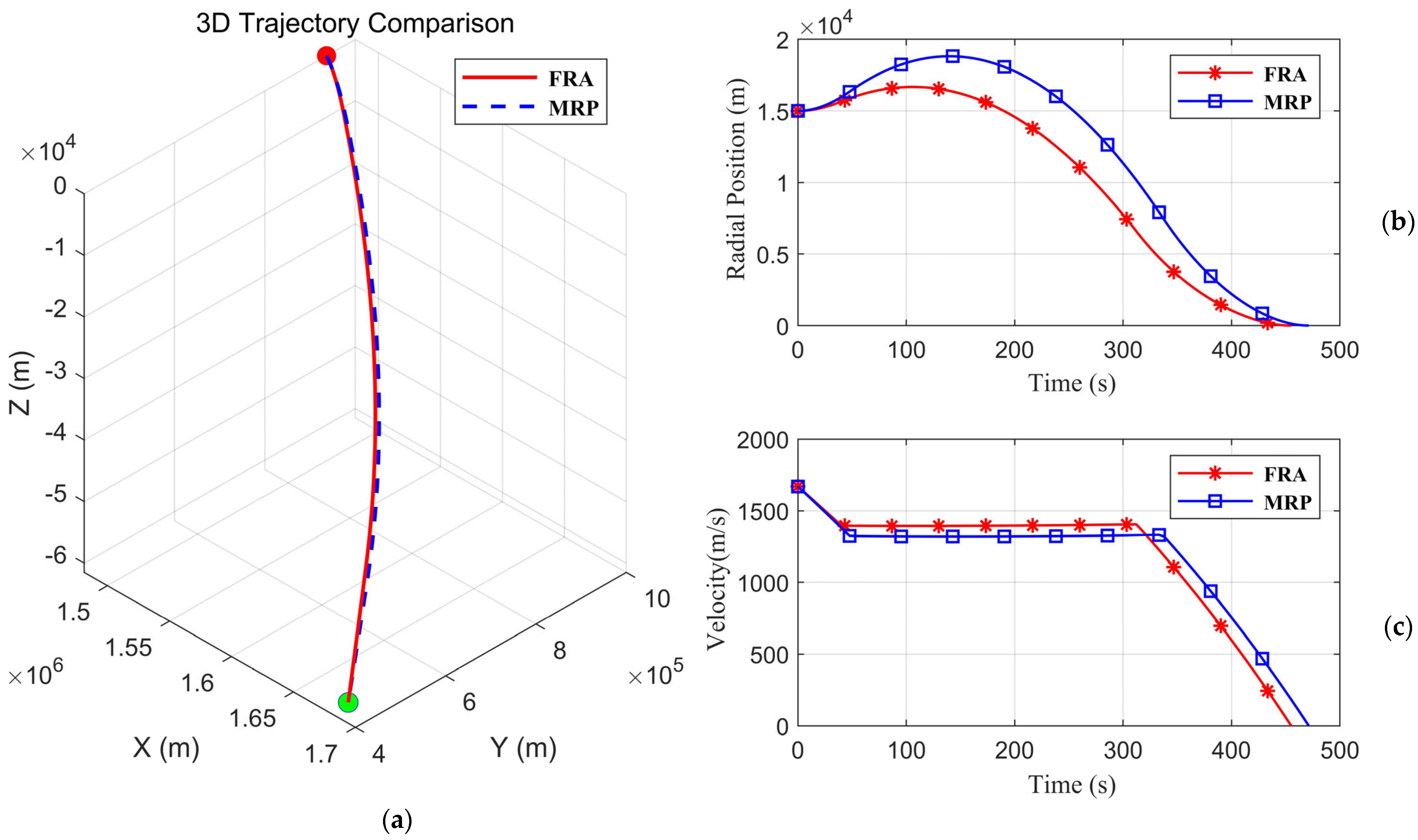
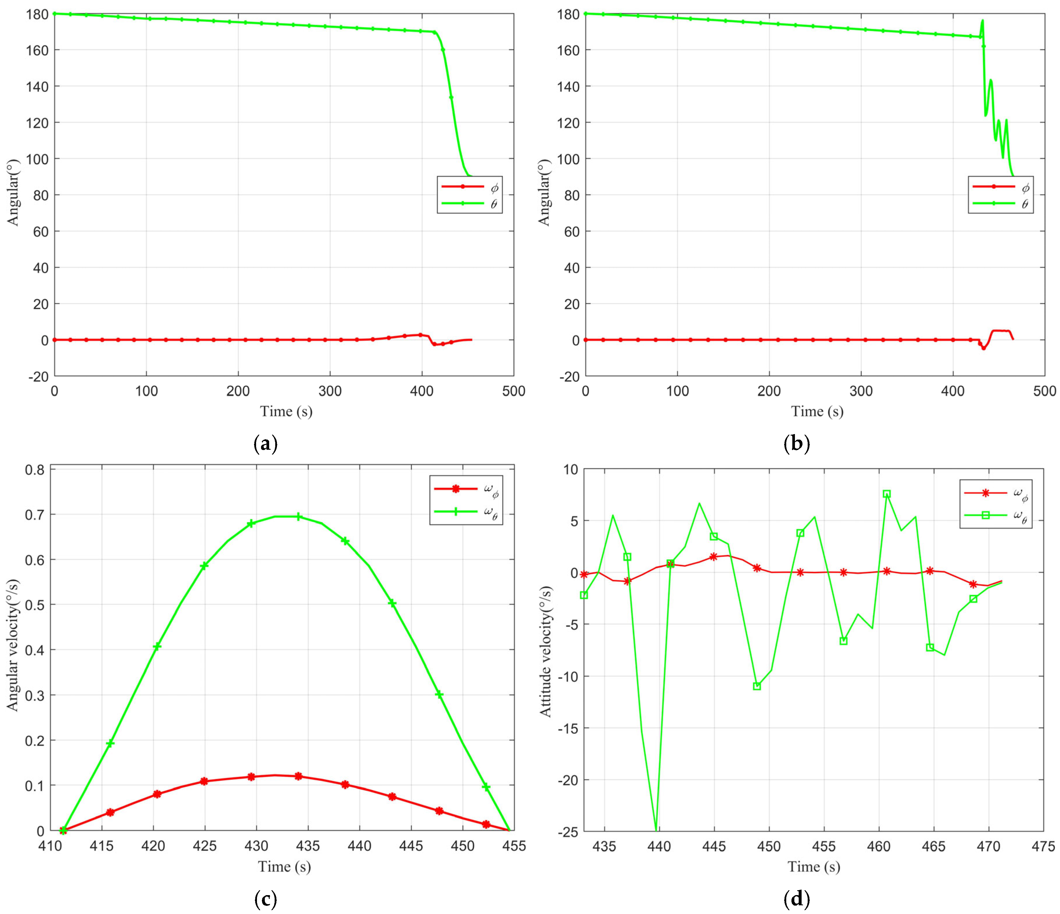
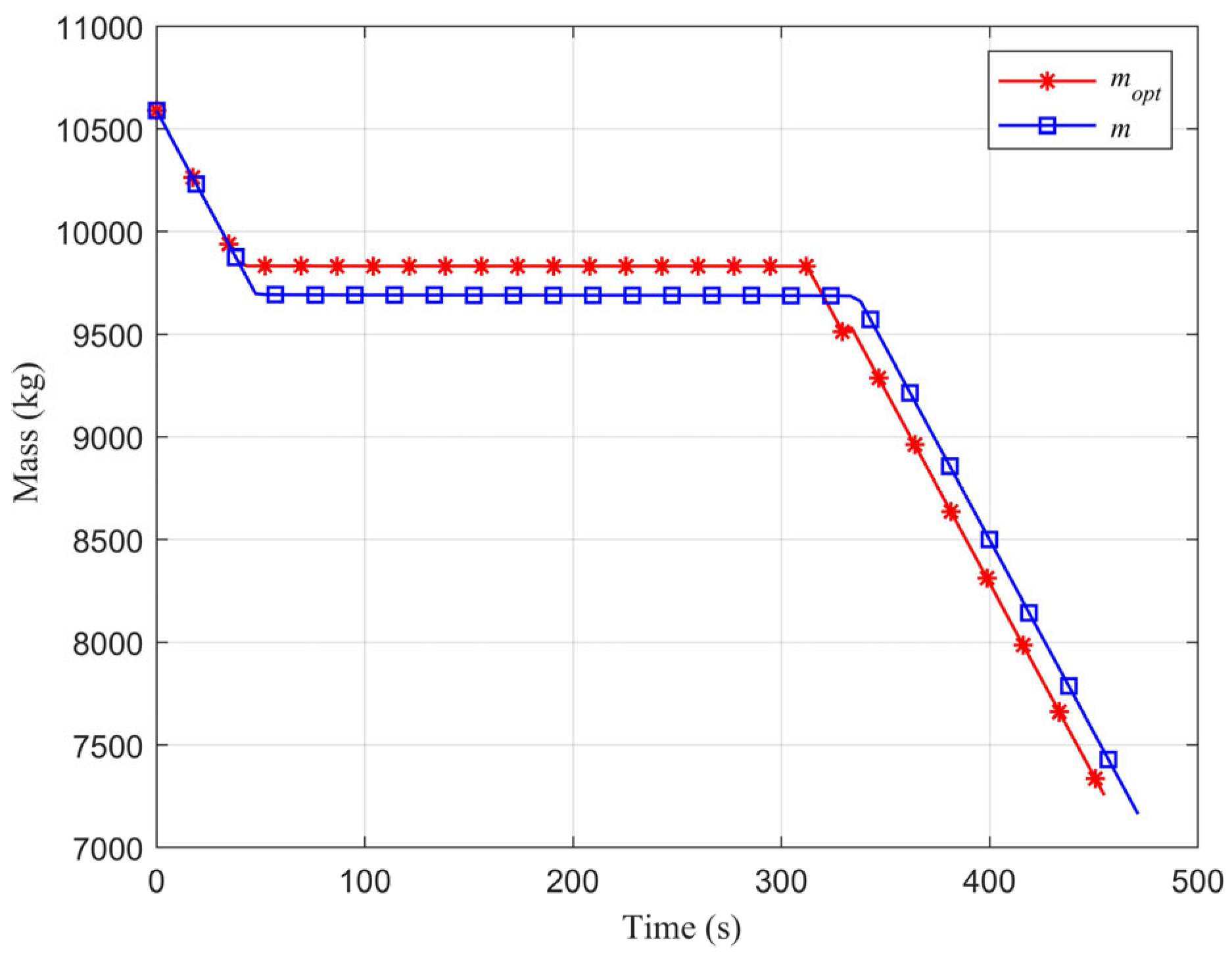
Figure 2, Figure 3 and Figure 4 present a comparative analysis of the 6-DOF landing trajectories generated by the two methods, where the red curves denote the modified FRA method and the blue curves denote the MRP method. In Figure 2a, which illustrates the three-dimensional trajectories, both methods successfully achieve a pinpoint soft landing. However, the modified method reduces the total landing time to 454.65 s, compared with 471.21 s for the MRP method, yielding a reduction of 16.56 s. The differences are further reflected in Figure 2b,c, where the radial position and radial velocity histories exhibit noticeable discrepancies, again demonstrating the shorter descent duration achieved by the modified method.

Figure 3 shows the attitude and angular velocity profiles obtained from the two methods. The modified method produces a significantly smoother attitude response, whose time history closely follows the polynomial trend defined in Equation (35) and asymptotically converges to 90° at approximately 445 s. This provides a sufficient time margin to establish and maintain a near-vertical attitude prior to touchdown. In contrast, the MRP-based method exhibits pronounced oscillations in the attitude profile and does not initiate a monotonic decrease until after 463 s, with an angular rate of approximately 1°/s.

Figure 4 presents the mass histories for both methods. The final landing masses are 7254.8 kg for the modified method and 7162.3 kg for the original method, indicating that the modified approach saves approximately 100 kg of propellant and achieves an improved fuel optimality.

The second case examines the sub-500 m trajectory and attitude profile. Using an initial mass of 8500 kg for the lander and the parameters in

Table 2. Problem parameters for the 6-DOF powered descent problem under 500 m.

Parameter	Value	Unit	Parameter	Value	Unit
m0	8500	kg	mf	4500	kg
r0	[500 300 500]T	m	v0	[100 0 0]T	m/s
rf	[0 0 0]T	m	vf	[0 0 0]T	m/s
Isp	460	s	ω0, ωf	[0 0 0]T	rad/s
θ0	[0 −60 0]T	deg	θf	[0 0 0]T	deg
Tmax	9000	N	Tmin	10,000	N

, the numerical solution utilized 30 collocation points (10 per mesh) and was allowed a maximum of 20 iterations.

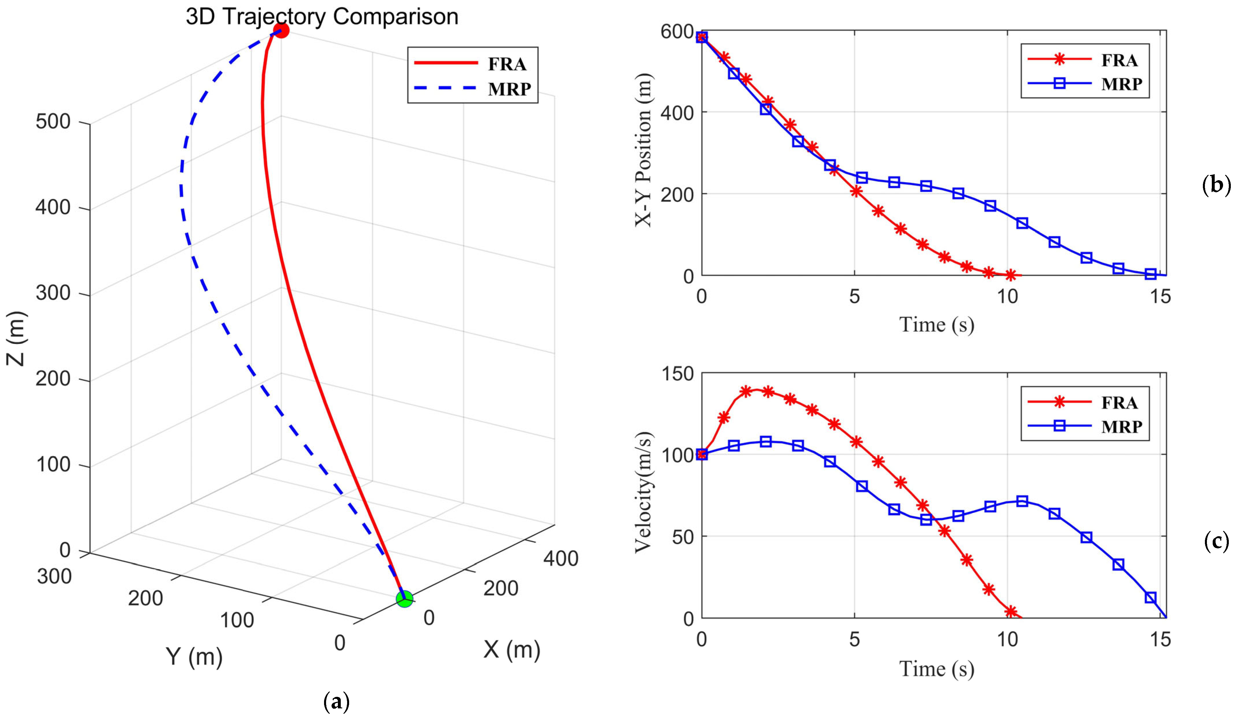
Figure 5, Figure 6 and Figure 7 present the state histories along the optimal landing trajectory below 500 m, including the position, velocity, attitude angles, and angular velocities. The results indicate that both methods satisfy the constraints of the trajectory planning problem. However, as shown in Figure 5a, the modified FRA method avoids trajectory overshoot and achieves a shorter landing time.

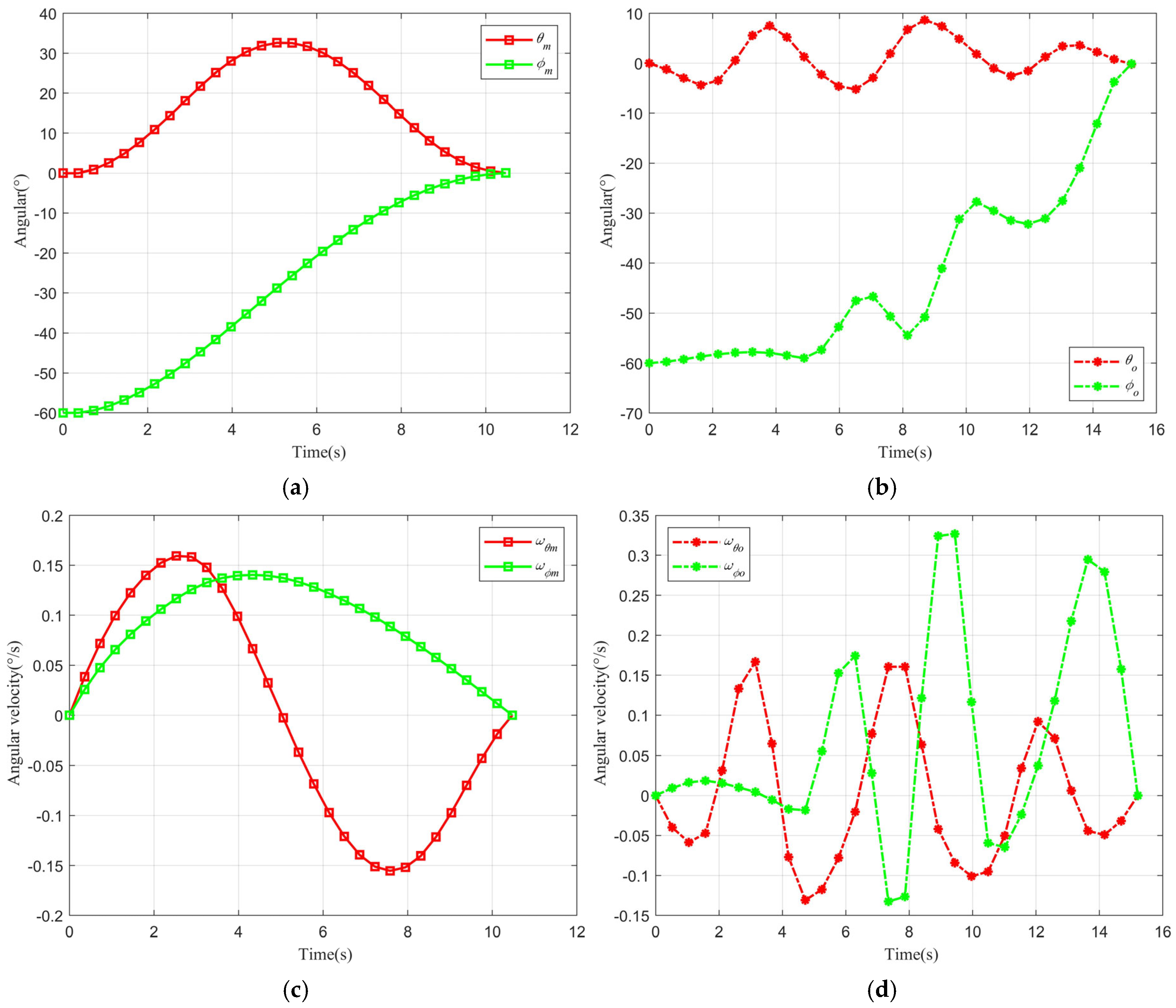
Figure 6 illustrates the attitude and angular velocity responses for both methods. The initial angle between the vehicle and the local horizontal plane is 60°, with the roll angle constrained to zero. As shown in Figure 6a,b, the attitude angle and angular velocity obtained from the modified FRA method follow the prescribed polynomial interpolation trend. In contrast, the MRP method does not exhibit a clear functional variation pattern in its attitude profile, and its angular velocity shows significant fluctuations over time, as seen in Figure 6d. Nevertheless, both methods satisfy the requirement for a vertical landing.

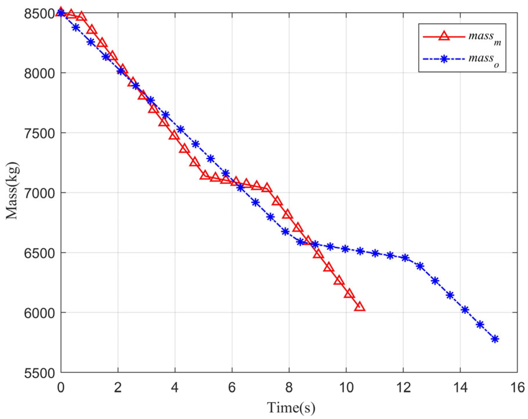
As indicated in Figure 7, the landing time of the MRP method is 15.37 s, which is 3.94 s longer than that of the modified method. The remaining propellant mass is 5739.2 kg for the MRP method and 6040.5 kg for the modified FRA method, demonstrating the improved fuel performance of the proposed approach.

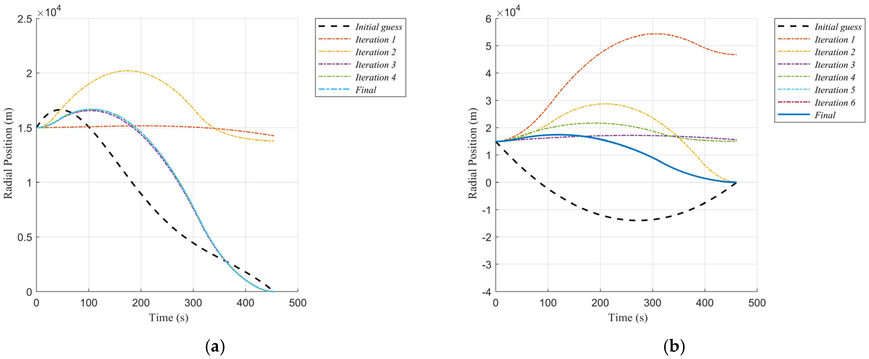
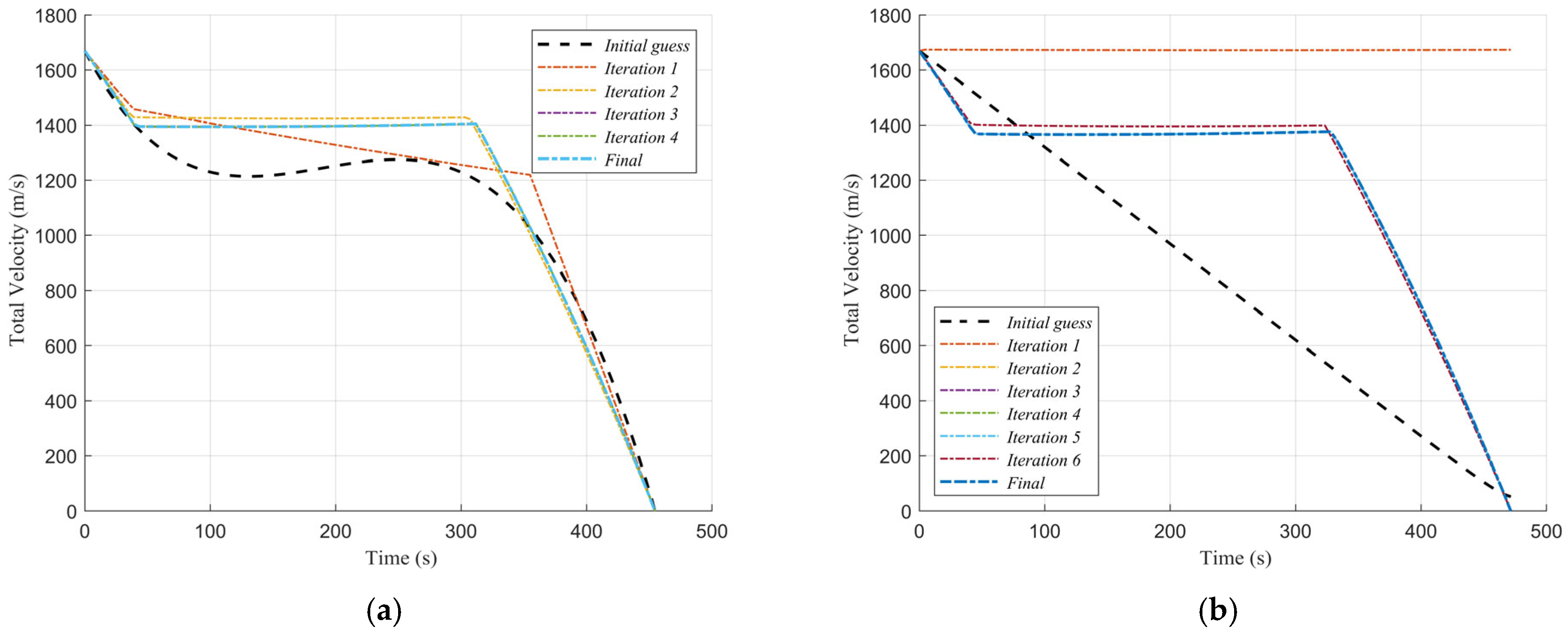
We further evaluate the impact of different initial guess strategies for the SCvx-based trajectory optimization. Two strategies are compared: the fast iterative gradient (FIG) initial guess method and the FOH (first-order hold) initial guess method. The convergence behaviors in Figure 8 and Figure 9 illustrate the convergence histories of the trajectory and velocity profiles over the entire powered descent phase under the two initial guesses. The FIG-based initial trajectory closely captures the global trend of the converged optimal solution in both position and velocity, thereby providing a physically consistent and numerically favorable starting point. In contrast, the FOH initial guess deviates substantially from the converged solution. This discrepancy is especially evident in the trajectory convergence history (Figure 8b), where the linear interpolation produces unphysical negative values, indicating a poor approximation and potential violation of basic physical feasibility. As a result, the FIG strategy converges in five iterations, whereas the FOH method requires seven iterations.

Table 3. Comparison of convergence metrics for SCvx with FIG and FOH initial guess strategies.

Method	Iterations	Objective	Maximum Violation	Virtual Control Norm	Time
Fast Iterative Gradient Initial Guess Method	1	−0.9978	1919.7	1.16 × 10−3	0.706
	2	−0.9576	528.02	2.15 × 10−5	0.661
	3	−0.9569	3.190	3.89 × 10−6	0.652
	4	−0.9567	2.102 × 10−6	3.99 × 10−6	0.648
	5	−0.9564	0	3.92 × 10−6	0.621
FOH Initial Guess Method	1	−0.9978	12,528	6.52 × 10−3	0.728
	3	−0.9576	5230	1.51 × 10−5	1.464
	4	−0.9579	405.58	5.34 × 10−5	1.399
	5	−0.9575	21.30	4.97 × 10−6	1.117
	6	−0.9575	0.944	4.68 × 10−6	0.899
	7	−0.9579	1.071 × 10−6	4.44 × 10−6	0.728

compares the SCvx convergence under two initial guess strategies (FIG vs. FOH) in terms of the objective value, constraint violation (defined as position error), virtual control norm, and runtime. Overall, the FIG initial guess provides a substantially better warm start, leading to faster and more robust convergence. Specifically, FIG reduces the maximum constraint violation much more rapidly (from 1919.7 at the first iteration to near zero by iteration 4) and reaches full feasibility in five iterations, whereas the FOH method starts from a significantly larger infeasibility (12,528) and requires seven iterations to achieve a comparable feasibility. Meanwhile, the objective value under FIG stabilizes earlier, indicating the quicker attainment of a high-quality solution. In addition, FIG shows a consistently lower and more stable computational time per iteration (about 0.62–0.71 s), while the FOH/linear approach experiences noticeably higher mid-iteration costs (exceeding 1.1 s), resulting in a lower overall efficiency. These results confirm that the FIG-based initial guess improves both the convergence speed and computational performance.

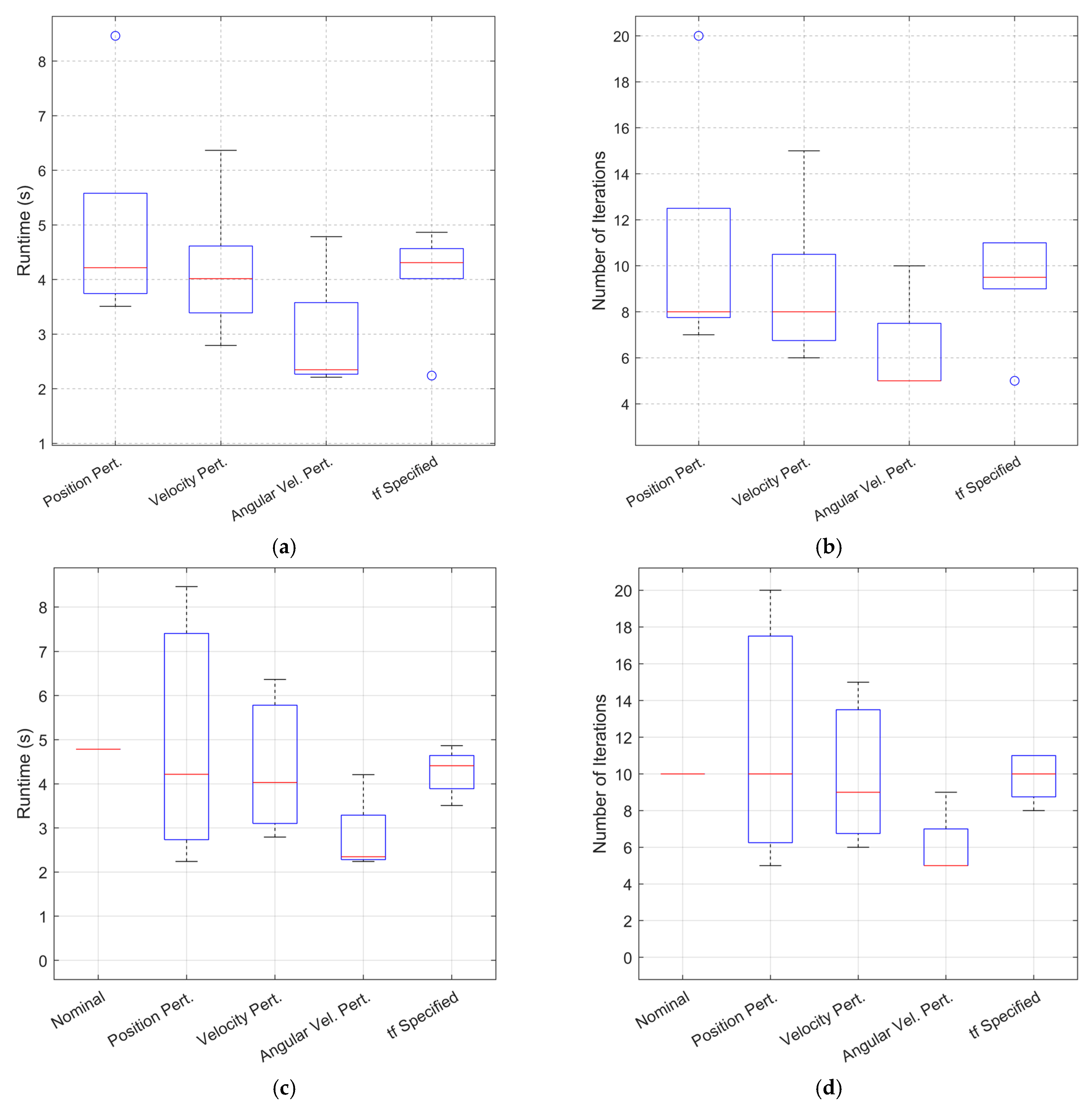
The second scenario compares trajectory planning strategies for a vehicle performing a major attitude maneuver below a 500 m altitude. A Monte Carlo study with 200 randomized cases was conducted, applying 10% perturbations to position, velocity, attitude, and angular velocity. The statistical results (

Table 4. Monte Carlo comparison of SCvx convergence performance under FIG and FOH initial guess strategies.

Method	Runtime, s	Iterations	Average Time per Iteration	Mean of Terminal Position	Mean and Standard Deviation of Fuel Consumption
FIG Initial Guess Method	4.088 ± 1.647 s	9.25 ± 4.01	0.447 ± 0.019	1.16 × 10−3	2409.5 ± 10.48
FOH Initial Guess Method	11.630 ± 0.275	20.00 ± 0.00	0.581 ± 0.014	6.52 × 10−3	2741.5 ± 1.48

) show that the FIG-based initialization significantly outperforms the FOH (linear interpolation) approach. Specifically, FIG reduces the average iteration count from 20.0 to 9.25 (−53.8%) and decreases the total runtime from 11.63 s to 4.09 s (−64.9%), while also improving the per-iteration efficiency by 23.2%.

Figure 10 further illustrates the categorized boxplot distributions of runtime and iteration counts. Both methods exhibit a differentiated sensitivity to disturbance types, with position perturbations causing the largest performance degradation and angular velocity perturbations having the least impact. However, the FIG-based method shows more compact distributions and a faster convergence. Notably, 90% of FIG cases converge within 13 iterations, and all cases converge within 20 iterations. Although FOH also achieves convergence in all cases, it exhibits a larger dispersion and greater sensitivity to translational perturbations.

Overall, while both methods demonstrate a satisfactory robustness under multi-dimensional uncertainties, the FIG-based initialization achieves a faster, more consistent, and computationally efficient convergence.

To quantitatively assess the smoothness improvement achieved by the modified FRA parameterization, the total variation (TV) and root-mean-square (RMS) metrics of the attitude rate and acceleration are reported in Table 5.

The total variation (TV) of the attitude rate is defined in discrete form as

$$TV\left({\omega }_i\right)={\displaystyle \sum _{k=1}^{N-1}\left|{\omega }_i^{k+1}-{\omega }_i^k\right|}$$

where ${\omega }_i^k$ denotes the angular rate of channel i at time node k.

Similarly, the total variation in the angular acceleration is defined as

$${\alpha }_i^k={\displaystyle \frac{{\omega }_i^{k+1}-{\omega }_i^k}{\Delta t_k}}$$

$$TV\left({\alpha }_i\right)={\displaystyle \sum _{k=1}^{N-1}\left|{\alpha }_i^{k+1}-{\alpha }_i^k\right|}$$

The root-mean-square (RMS) attitude rate is defined as

$$RMS\left({\omega }_i\right)=\sqrt{{\displaystyle \frac{1}{T}}{\displaystyle \underset{0}{\overset{T}{\int }}{\omega }_i^2\left(t\right)dt}}$$

which is approximated in discrete form as

$$RMS\left({\omega }_i\right)=\sqrt{{\displaystyle \frac{1}{N}}{\displaystyle \sum _{k=1}^{N-1}{\omega }_i^2\left(t_k\right)}}$$

As summarized in Table 5, the modified FRA parameterization consistently improves the smoothness across all quantitative indicators compared with the conventional MRP-based formulation. The discrete total variation (TV) of the attitude rate is reduced from 11.16 to 2.20 deg/s in the φ channel (80.3% reduction) and from 138.29 to 6.62 deg/s in the θ channel (95.2% reduction).

More substantial improvements are observed in the total variation in the angular acceleration, which decreases by 90.6% in the φ channel and 98.3% in the θ channel, corresponding to a more than one order of magnitude suppression of oscillatory components.

In terms of RMS metrics, the attitude rate magnitude decreases by approximately 77% in both channels, while the RMS attitude acceleration in the φ channel is reduced by 86.6%. Although the RMS acceleration in the θ channel remains at a comparable level, its total variation decreases by over 98%, indicating that the FRA-based parameterization effectively attenuates the high-frequency fluctuations and sharp transitions observed in the MRP-based solution.

Overall, these results demonstrate that the FRA formulation significantly enhances trajectory smoothness and numerical stability, yielding more physically consistent attitude profiles.

Table 5. Quantitative comparison of attitude smoothness metrics (TV and RMS) under different parameterizations.

Initial Condition	Method	TV(ω)	TV(α) [deg/s2]	RMS(ω) [deg/s]	RMS(α) [deg/s2]
φ = 0°	FRA	2.2015	1.1296	0.0956	0.0296
	MRP	11.1556	11.9566	0.4216	0.2215
θ = 60°	FRA	6.6241	3.1060	0.8923	0.0784
	MRP	138.2900	180.0509	3.7826	3.1124

Table 5. Quantitative comparison of attitude smoothness metrics (TV and RMS) under different parameterizations.

Initial Condition	Method	TV(ω)	TV(α) [deg/s2]	RMS(ω) [deg/s]	RMS(α) [deg/s2]
φ = 0°	FRA	2.2015	1.1296	0.0956	0.0296
	MRP	11.1556	11.9566	0.4216	0.2215
θ = 60°	FRA	6.6241	3.1060	0.8923	0.0784
	MRP	138.2900	180.0509	3.7826	3.1124

5. Conclusions

This manuscript presents an improved gradient-based sequential convex programming method for 6-DOF fuel optimization trajectory planning during the powered descent phase of a lunar lander, incorporating a normalized finite rotation angle formulation to describe rotation dynamics. Prior to discretization, the initial reference trajectory was estimated using a fast iterative gradient-based scheme, which evaluated the projection-analogous gradient in the iterative process. Two numerical case studies demonstrated that, compared to the MRP method, the proposed approach significantly reduced the number of attitude maneuvers, smoothed the attitude curve, and expanded the range of feasible attitude trajectories. Furthermore, compared to the linear initial value guessing, the new method reduced the number of iterations, the runtime, and the fuel consumption.