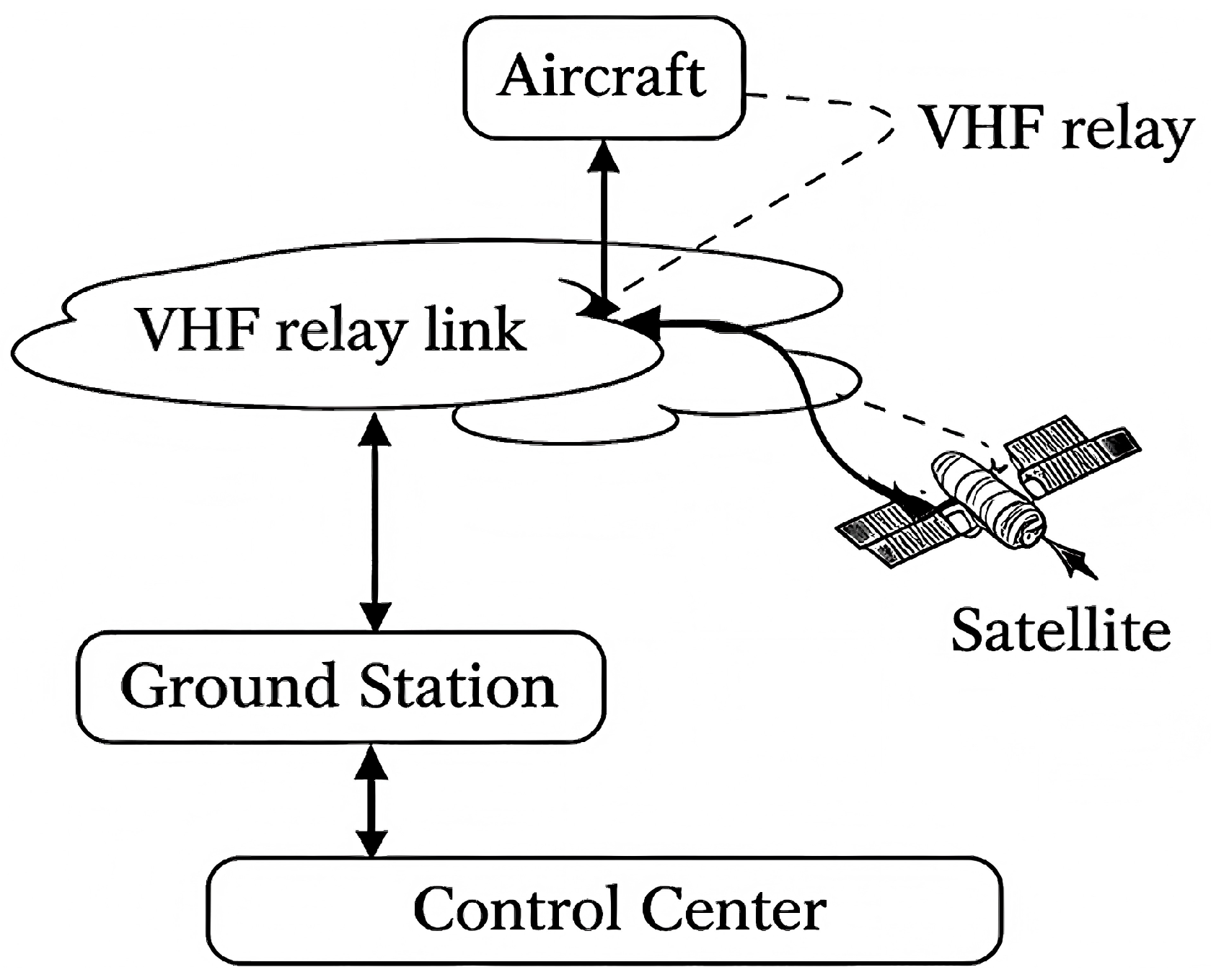
Figure 1.
Simplified architecture of a typical civil aviation VHF communication system.
Figure 1.
Simplified architecture of a typical civil aviation VHF communication system.
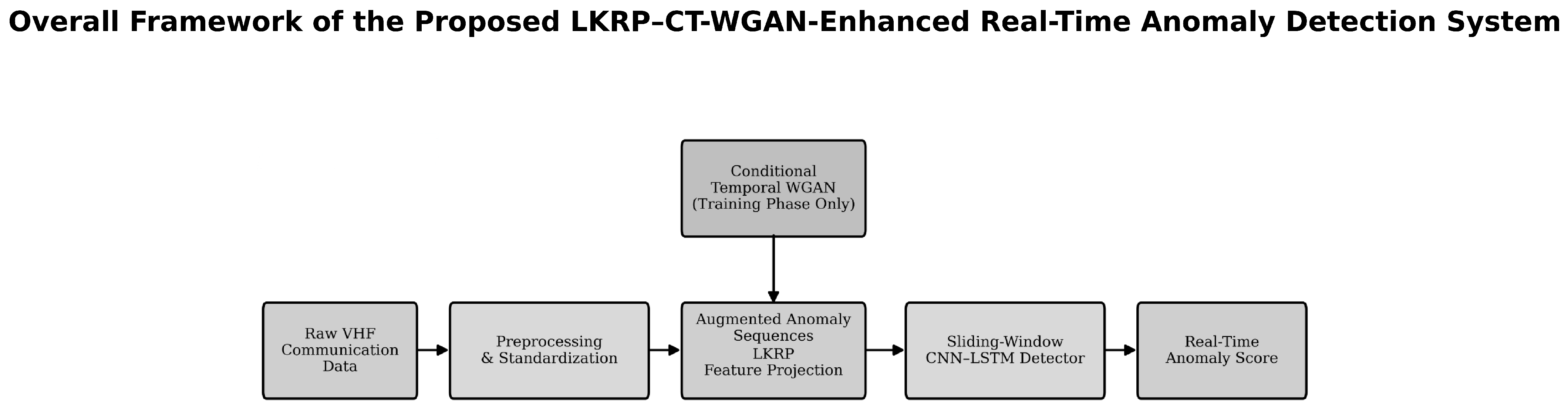
Figure 2.
Overview of the LKRP–CT–WGAN–CNN–LSTM pipeline for real-time anomaly detection in civil aviation VHF communication systems. The framework combines learnable nonlinear feature projection, condition-aware temporal augmentation, and hybrid spatiotemporal detection under severe class imbalance and strict avionics latency requirements.
Figure 2.
Overview of the LKRP–CT–WGAN–CNN–LSTM pipeline for real-time anomaly detection in civil aviation VHF communication systems. The framework combines learnable nonlinear feature projection, condition-aware temporal augmentation, and hybrid spatiotemporal detection under severe class imbalance and strict avionics latency requirements.
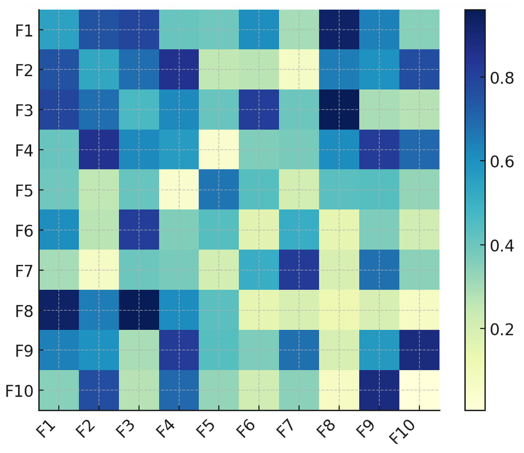
Figure 3.
Mutual information matrix among the MRMR-selected features, computed on the training set after LKRP pretraining. The results show reduced redundancy and strong relevance of the retained LKRP components.
Figure 3.
Mutual information matrix among the MRMR-selected features, computed on the training set after LKRP pretraining. The results show reduced redundancy and strong relevance of the retained LKRP components.
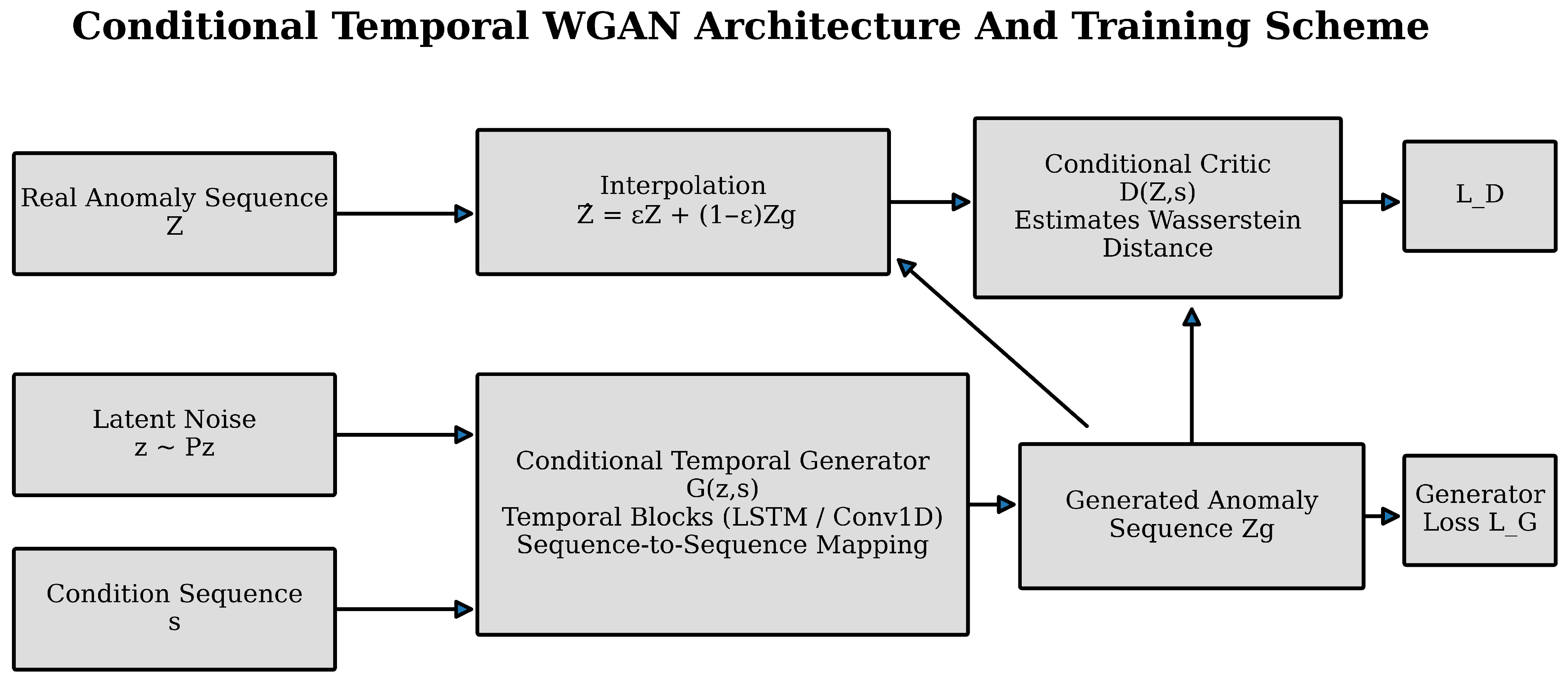
Figure 4.
Architecture of the conditional temporal WGAN (CT–WGAN). The generator produces anomaly-like temporal sequences conditioned on communication-state variables, while the critic enforces temporal realism and condition consistency through Wasserstein adversarial training.
Figure 4.
Architecture of the conditional temporal WGAN (CT–WGAN). The generator produces anomaly-like temporal sequences conditioned on communication-state variables, while the critic enforces temporal realism and condition consistency through Wasserstein adversarial training.
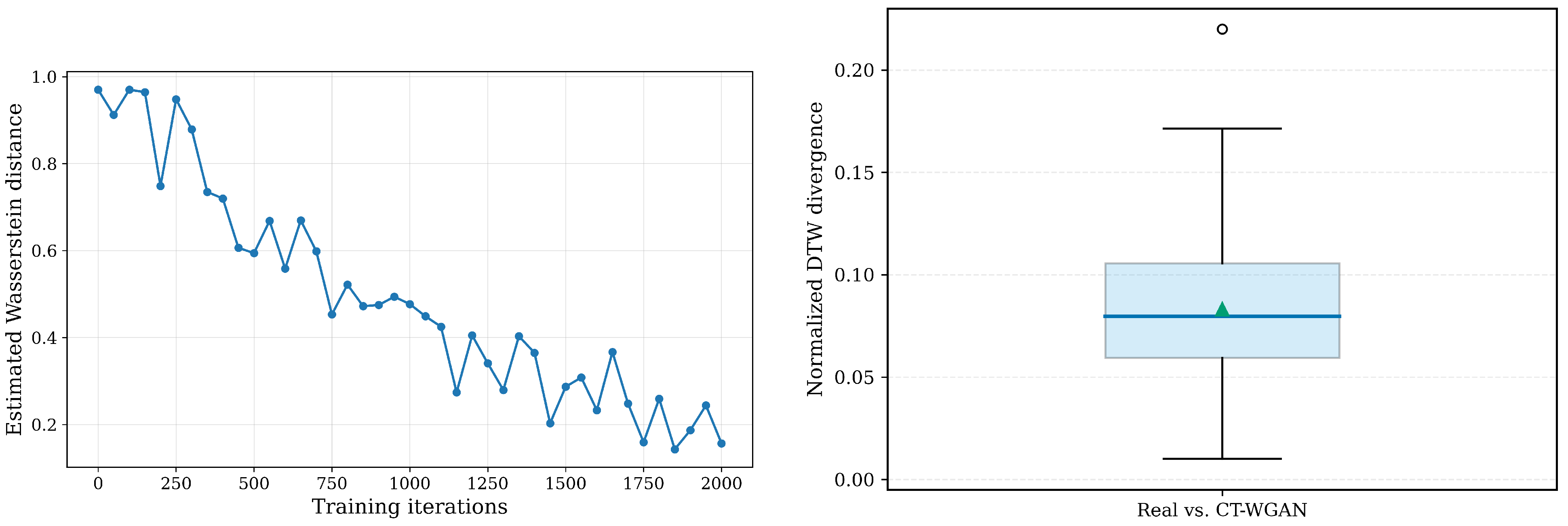
Figure 5.
CT–WGAN training dynamics and condition consistency. (Left): Wasserstein distance convergence during training. (Right): DTW-based condition consistency between real and generated sequences. Circles denote real anomaly sequences and triangles denote generated sequences.
Figure 5.
CT–WGAN training dynamics and condition consistency. (Left): Wasserstein distance convergence during training. (Right): DTW-based condition consistency between real and generated sequences. Circles denote real anomaly sequences and triangles denote generated sequences.
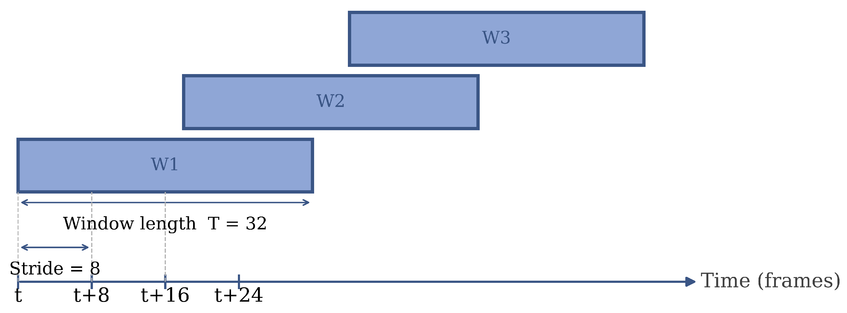
Figure 6.
Sliding window construction for sequential anomaly detection. Overlapping windows are generated from LKRP feature sequences and labeled as anomalous if any frame within the window is abnormal.
Figure 6.
Sliding window construction for sequential anomaly detection. Overlapping windows are generated from LKRP feature sequences and labeled as anomalous if any frame within the window is abnormal.
Figure 7.
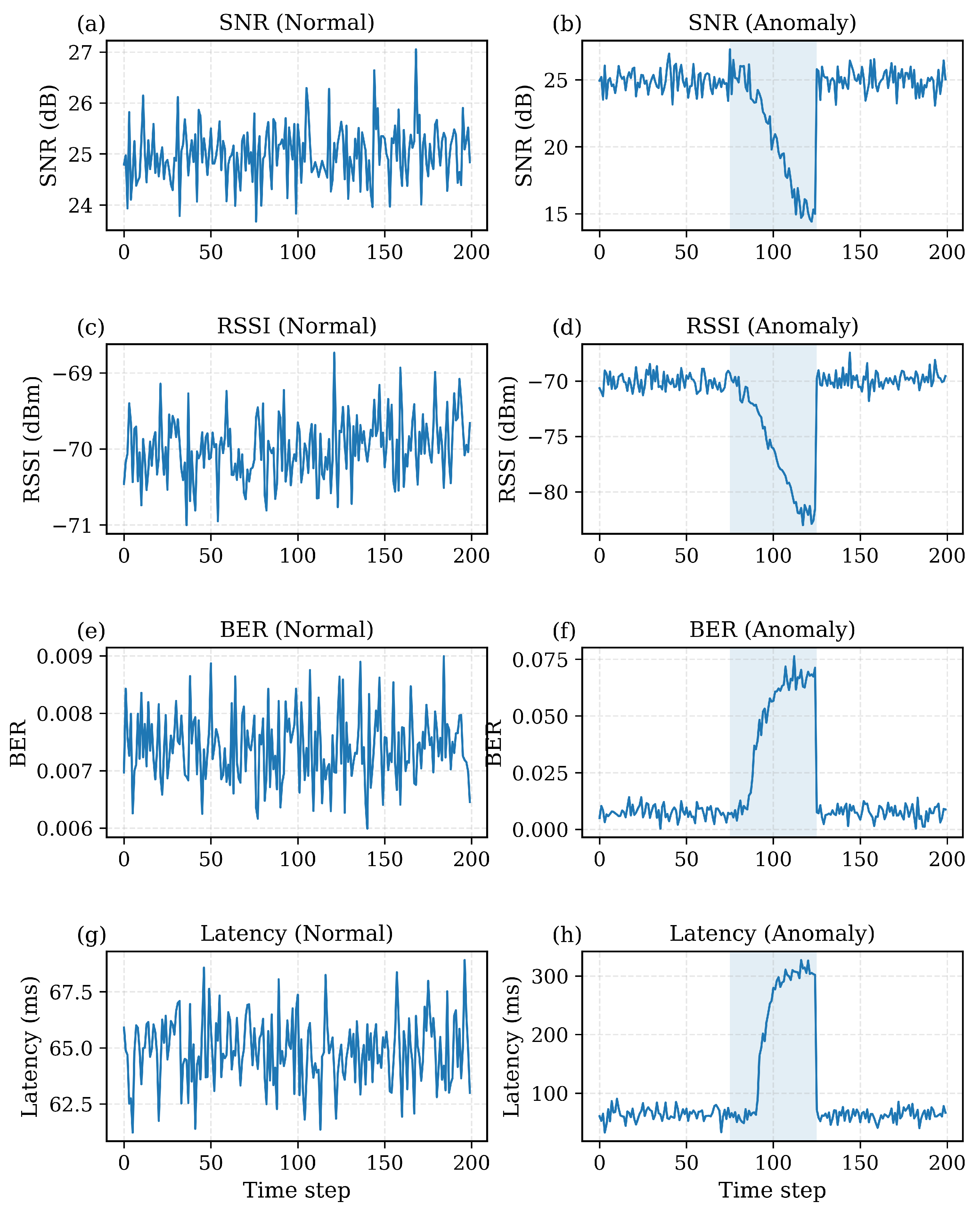
(a,b) Signal-to-noise ratio (SNR), (c,d) received signal strength indicator (RSSI), (e,f) bit error rate (BER), and (g,h) end-to-end latency. The left column corresponds to normal communication, and the right column shows an anomaly interval (shaded region). During the anomaly, RSSI decreases, followed by a delayed reduction in SNR, a rapid increase in BER, and a pronounced rise in latency.
Figure 7.
(a,b) Signal-to-noise ratio (SNR), (c,d) received signal strength indicator (RSSI), (e,f) bit error rate (BER), and (g,h) end-to-end latency. The left column corresponds to normal communication, and the right column shows an anomaly interval (shaded region). During the anomaly, RSSI decreases, followed by a delayed reduction in SNR, a rapid increase in BER, and a pronounced rise in latency.
Figure 8.
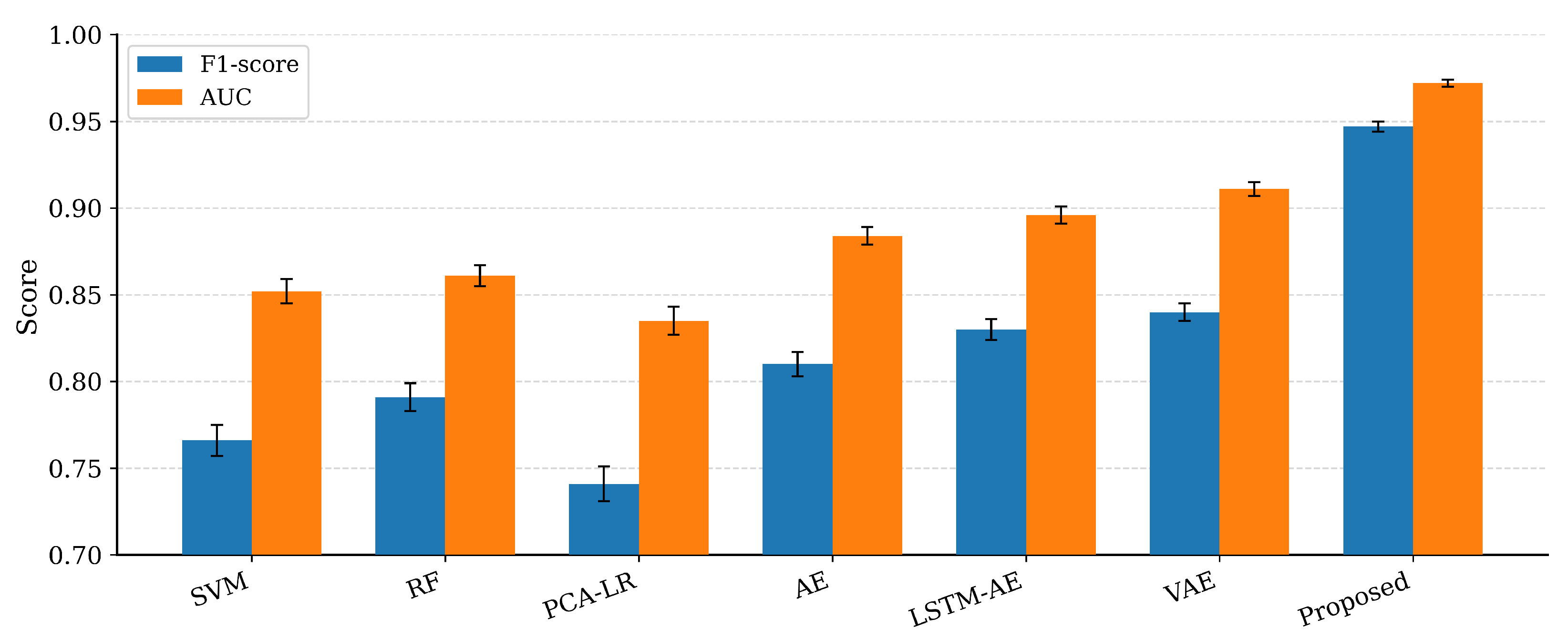
Overall comparison of anomaly detection methods in terms of F1-score and AUC.
Figure 8.
Overall comparison of anomaly detection methods in terms of F1-score and AUC.
Figure 9.
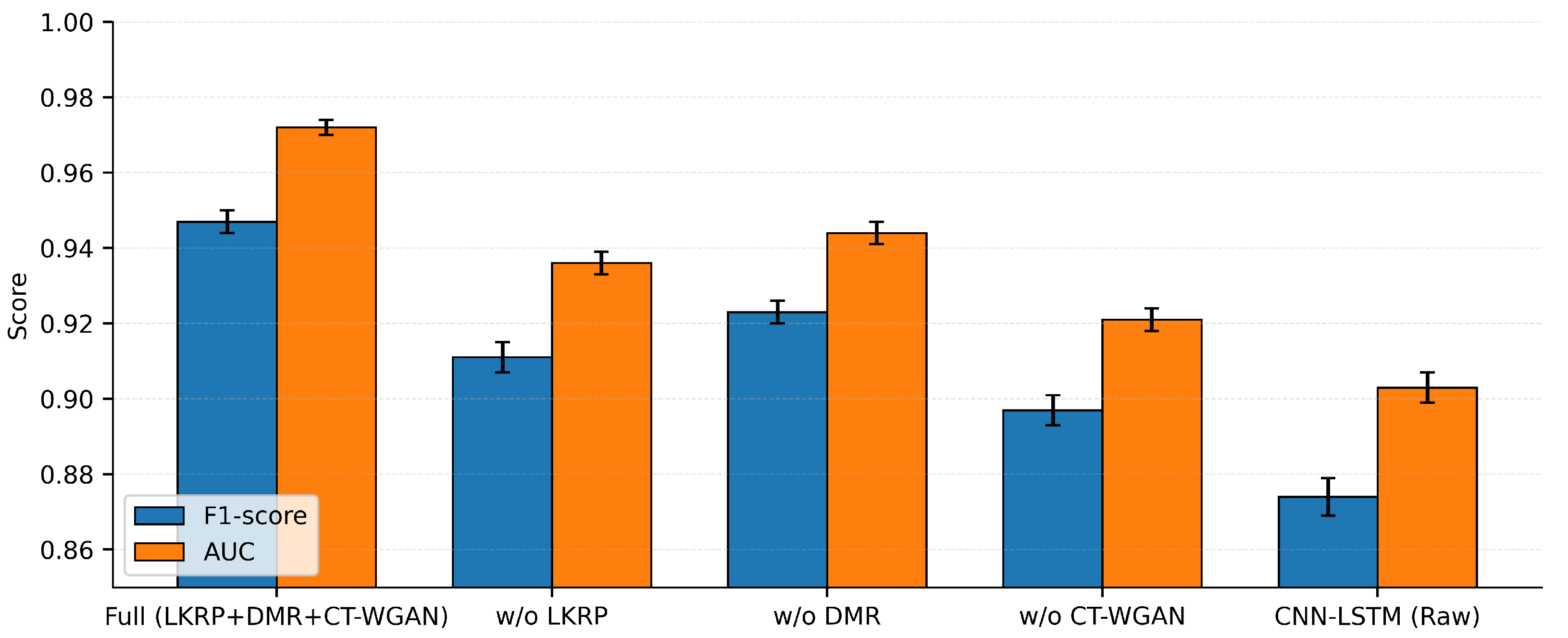
Ablation study results measured by F1-score and AUC. The full model shows the highest and most stable performance. Removing LKRP, DMR, or CT–WGAN leads to noticeable degradation. Error bars denote standard deviation.
Figure 9.
Ablation study results measured by F1-score and AUC. The full model shows the highest and most stable performance. Removing LKRP, DMR, or CT–WGAN leads to noticeable degradation. Error bars denote standard deviation.
Figure 10.
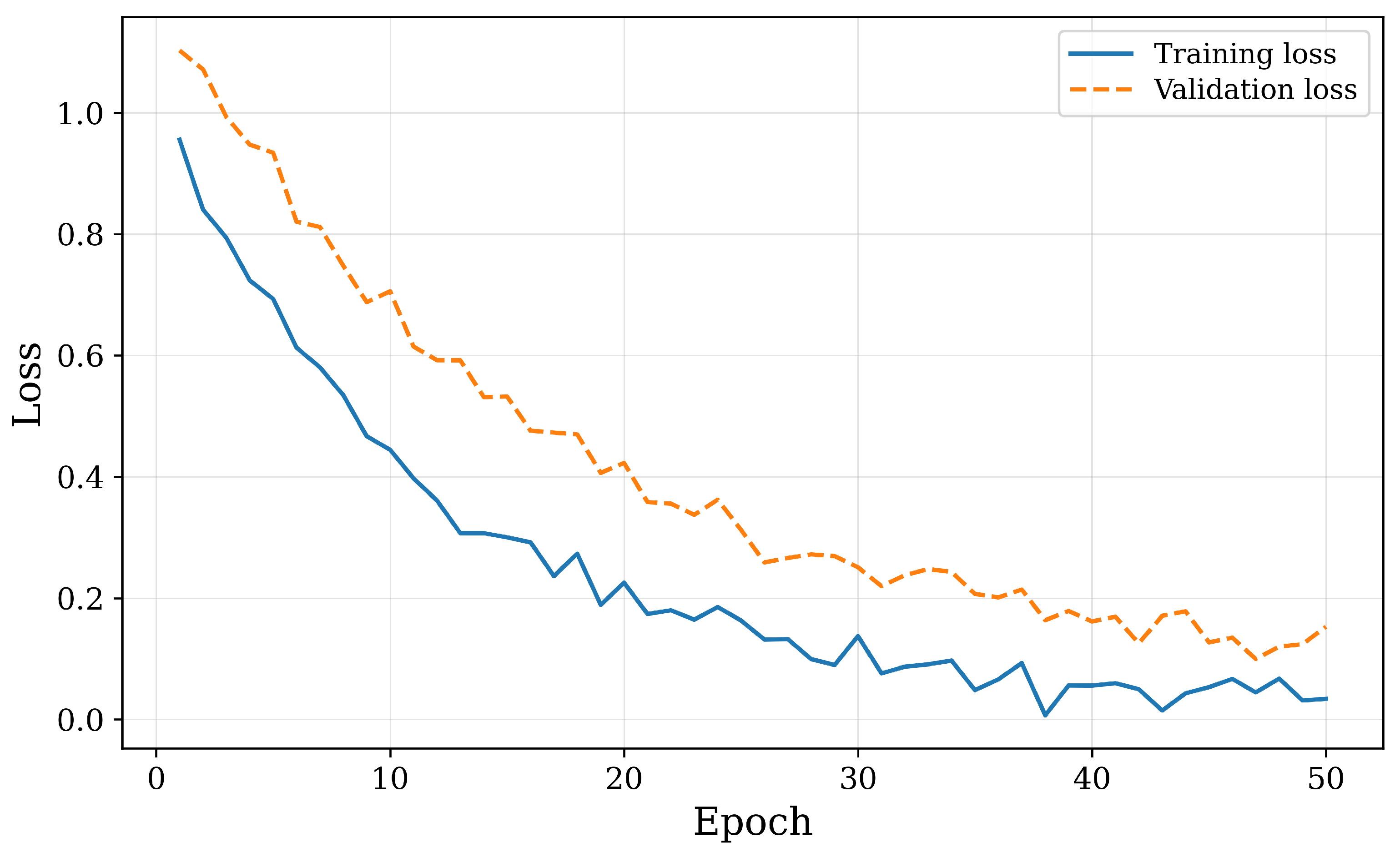
Training and validation loss curves for the CNN–LSTM detector.
Figure 10.
Training and validation loss curves for the CNN–LSTM detector.
Figure 11.
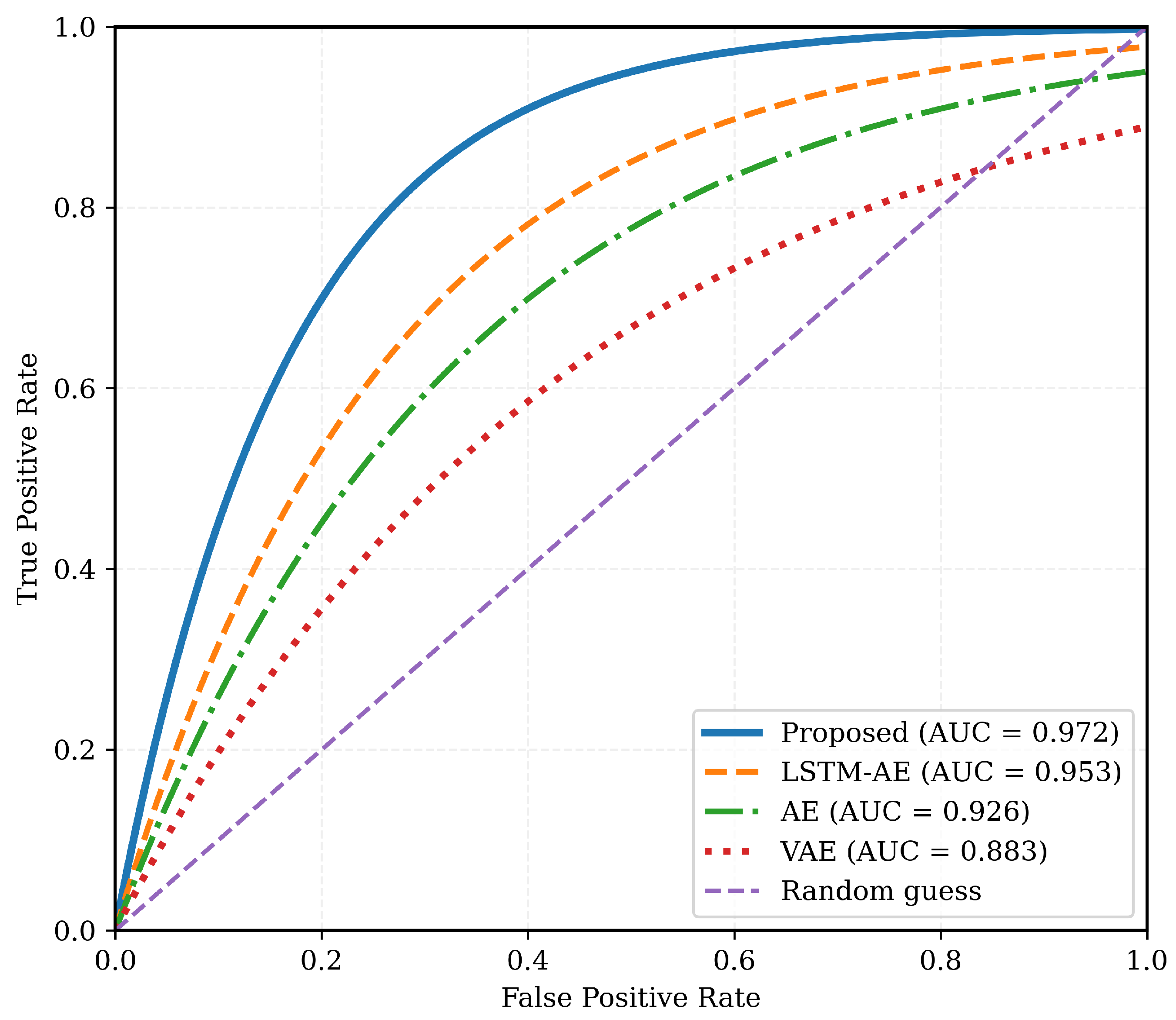
ROC curves comparing the proposed framework with baseline methods. The proposed model achieves the highest ROC-AUC. The diagonal dashed line corresponds to a random classifier.
Figure 11.
ROC curves comparing the proposed framework with baseline methods. The proposed model achieves the highest ROC-AUC. The diagonal dashed line corresponds to a random classifier.
Figure 12.
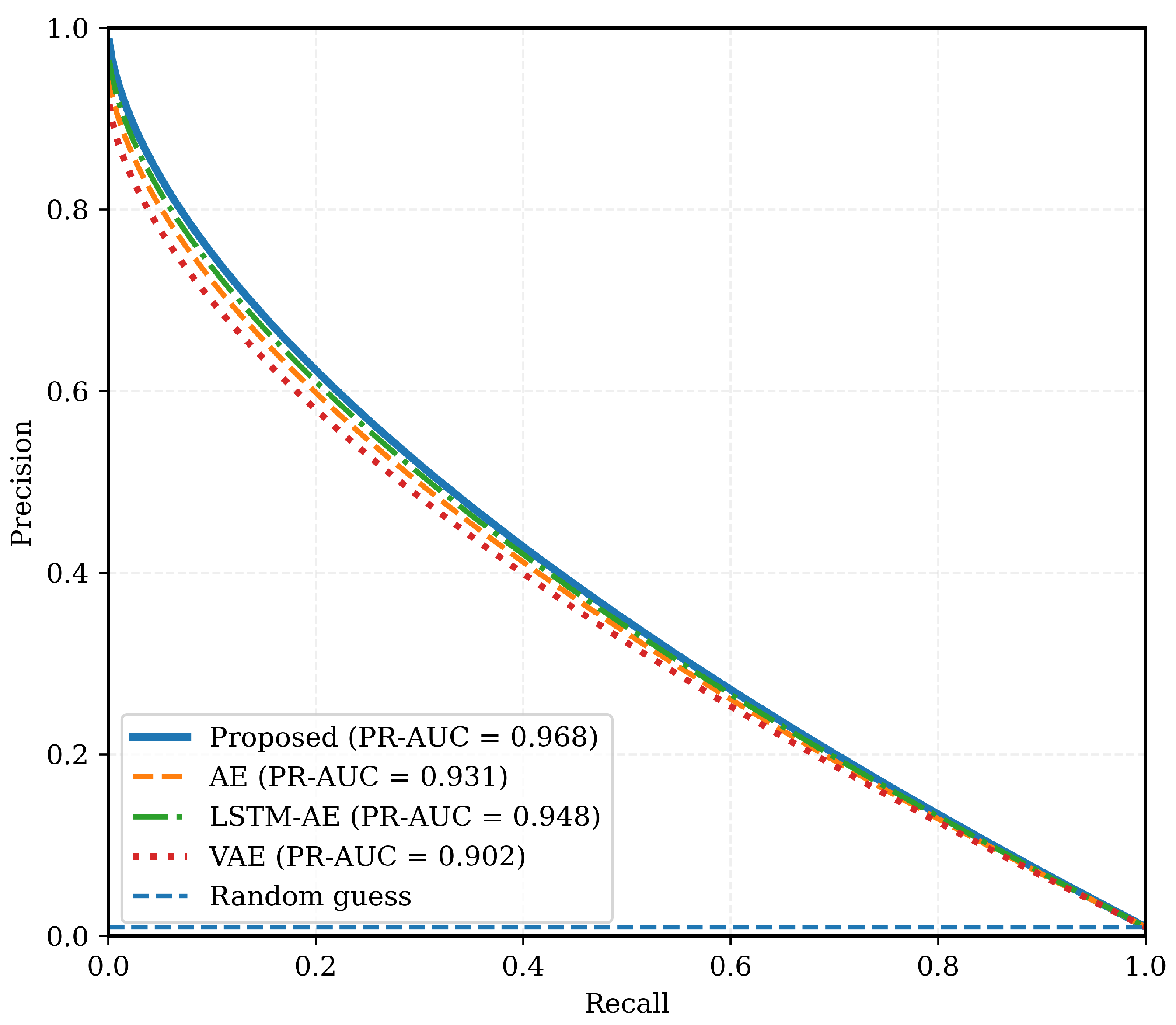
Precision–Recall curves comparing the proposed framework with baseline methods. The proposed model achieves the highest PR-AUC and maintains superior precision across the full recall range. The dashed horizontal line denotes the performance of a random classifier under the observed anomaly ratio.
Figure 12.
Precision–Recall curves comparing the proposed framework with baseline methods. The proposed model achieves the highest PR-AUC and maintains superior precision across the full recall range. The dashed horizontal line denotes the performance of a random classifier under the observed anomaly ratio.
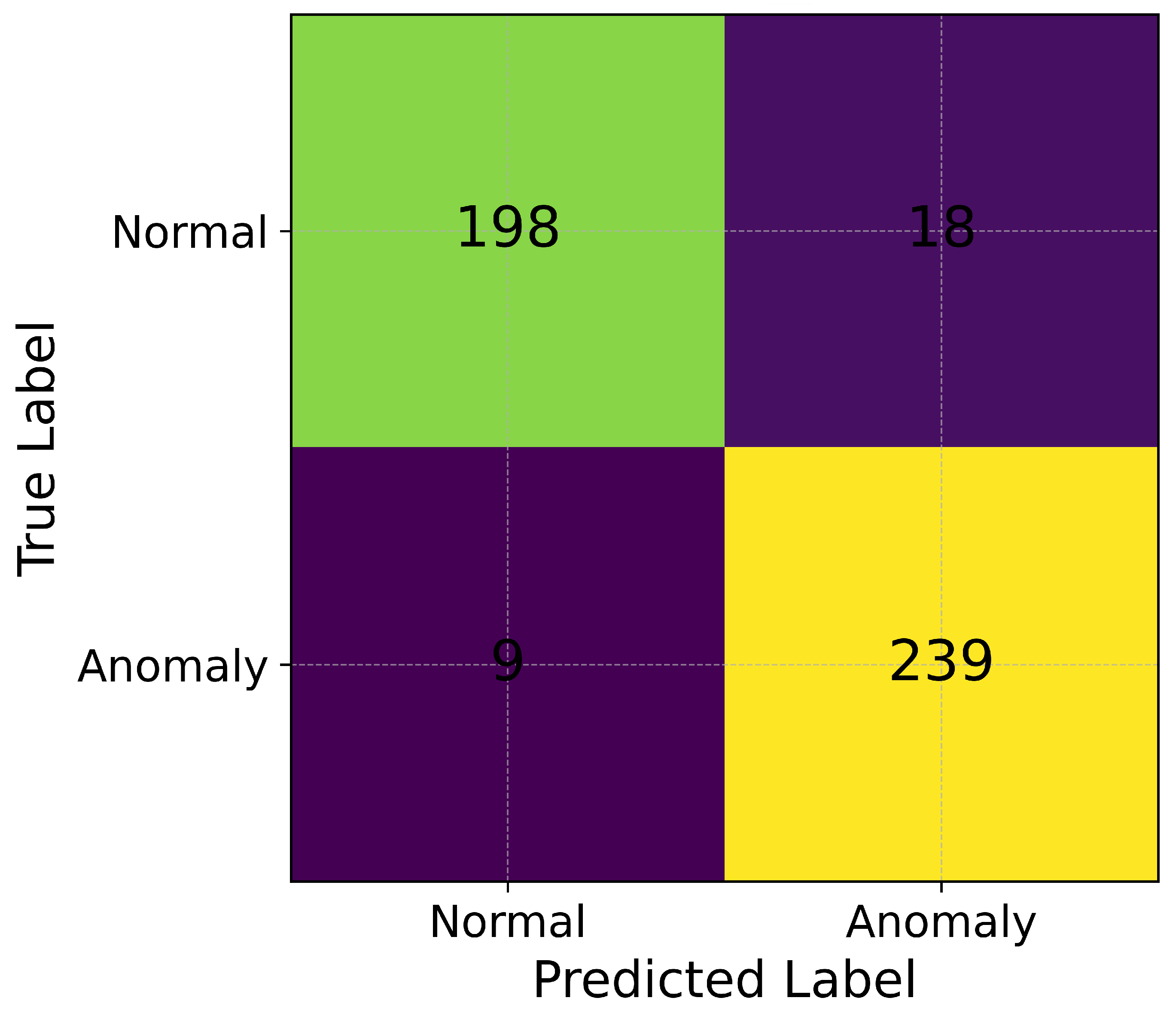
Figure 13.
Confusion matrix of the proposed framework on the window-level test set.
Figure 13.
Confusion matrix of the proposed framework on the window-level test set.
Figure 14.
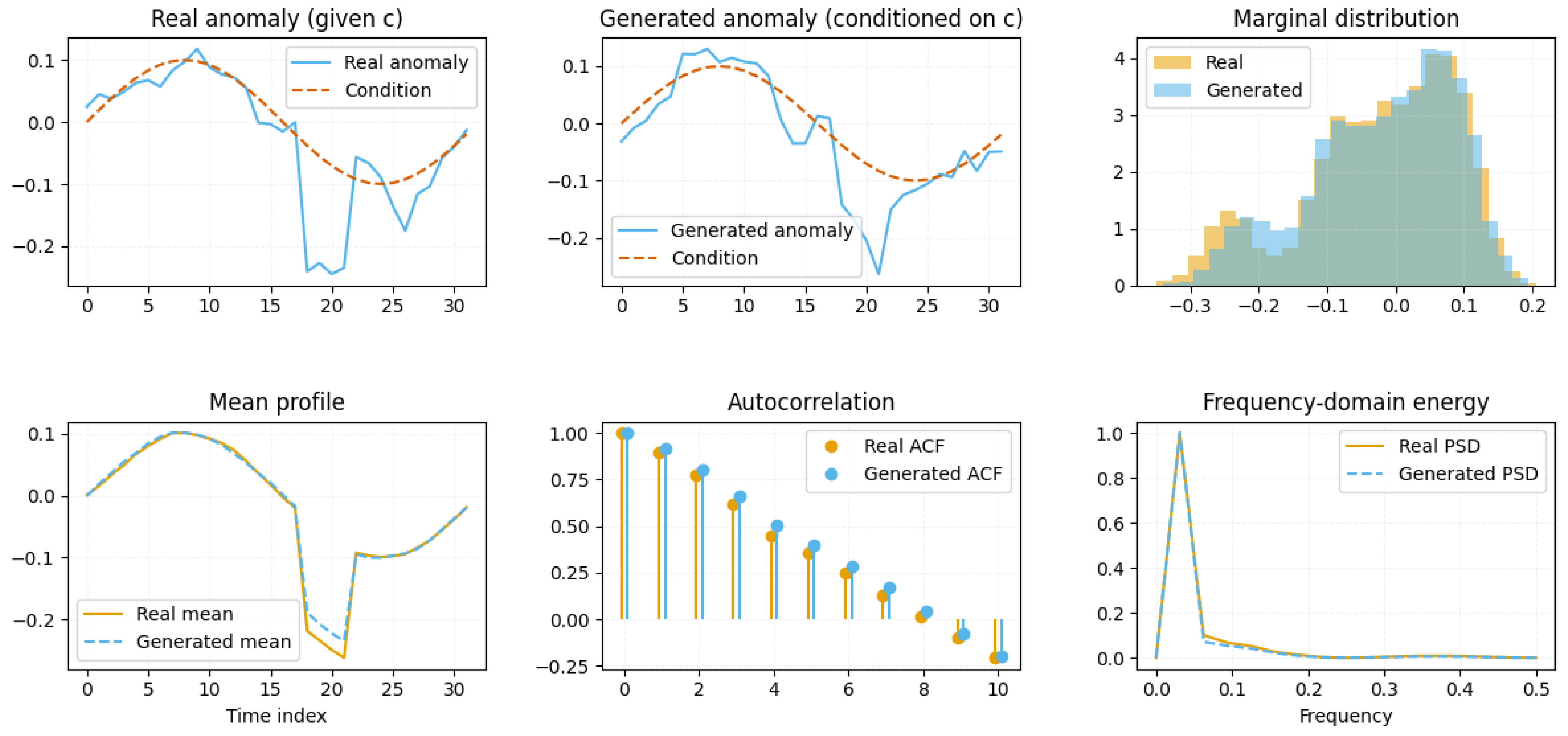
Statistical comparison between real and CT–WGAN generated anomaly sequences. Real and generated samples are compared in the time domain, distributional statistics, temporal correlations, and frequency-domain energy. The generated anomalies closely follow the real anomaly characteristics while maintaining slight variations, indicating realistic yet non-identical generation.
Figure 14.
Statistical comparison between real and CT–WGAN generated anomaly sequences. Real and generated samples are compared in the time domain, distributional statistics, temporal correlations, and frequency-domain energy. The generated anomalies closely follow the real anomaly characteristics while maintaining slight variations, indicating realistic yet non-identical generation.
Figure 15.
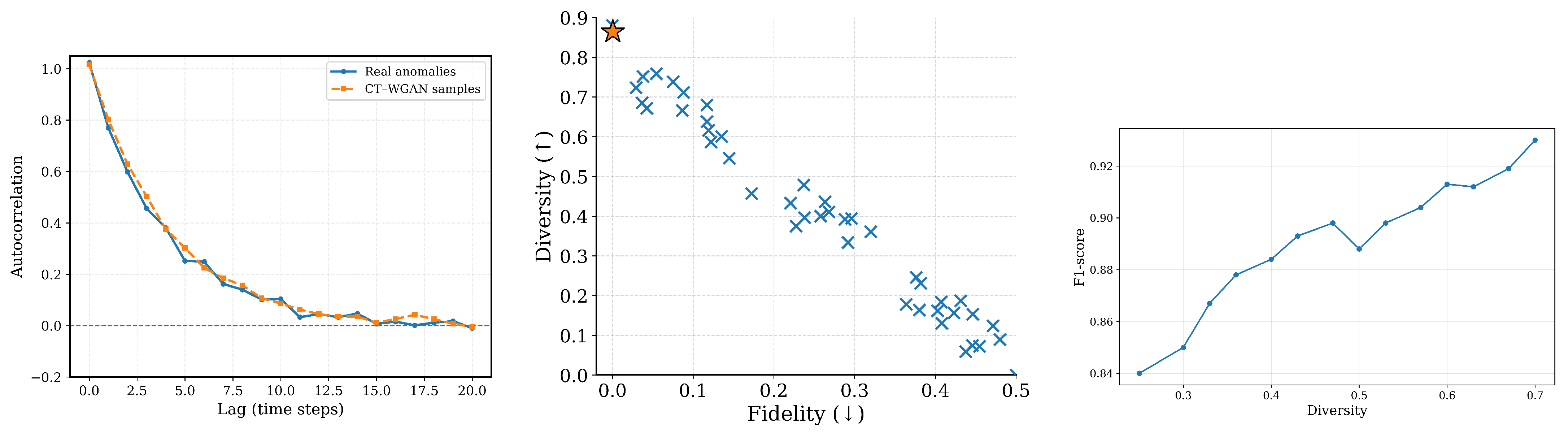
Quality assessment of CT–WGAN generated anomalies: ACF consistency (left), diversity–fidelity scatter (middle), and Diversity–F1 Pareto frontier (right). The dotted line in the left panel indicates the reference autocorrelation of real sequences. The asterisk in the middle panel denotes the selected operating point, and the arrow indicates the Pareto improvement direction.
Figure 15.
Quality assessment of CT–WGAN generated anomalies: ACF consistency (left), diversity–fidelity scatter (middle), and Diversity–F1 Pareto frontier (right). The dotted line in the left panel indicates the reference autocorrelation of real sequences. The asterisk in the middle panel denotes the selected operating point, and the arrow indicates the Pareto improvement direction.
Figure 16.
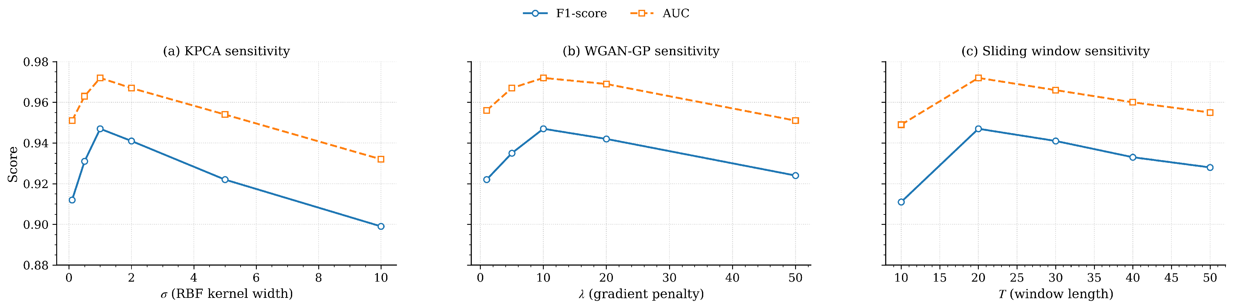
Sensitivity analysis of key hyperparameters, including LKRP kernel width , CT–WGAN penalty coefficient , and sliding window length T.
Figure 16.
Sensitivity analysis of key hyperparameters, including LKRP kernel width , CT–WGAN penalty coefficient , and sliding window length T.
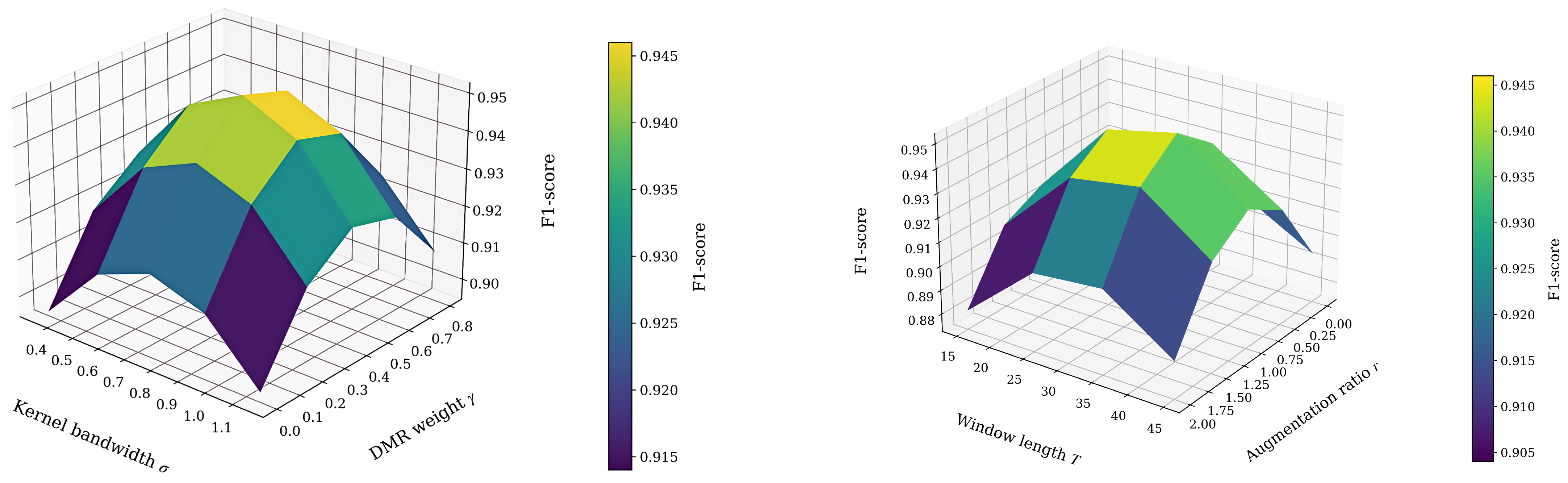
Figure 17.
Joint hyperparameter interaction analysis. (Left): LKRP kernel bandwidth vs. DMR weight . (Right): CT–WGAN augmentation ratio r vs. window length T.
Figure 17.
Joint hyperparameter interaction analysis. (Left): LKRP kernel bandwidth vs. DMR weight . (Right): CT–WGAN augmentation ratio r vs. window length T.
Figure 18.
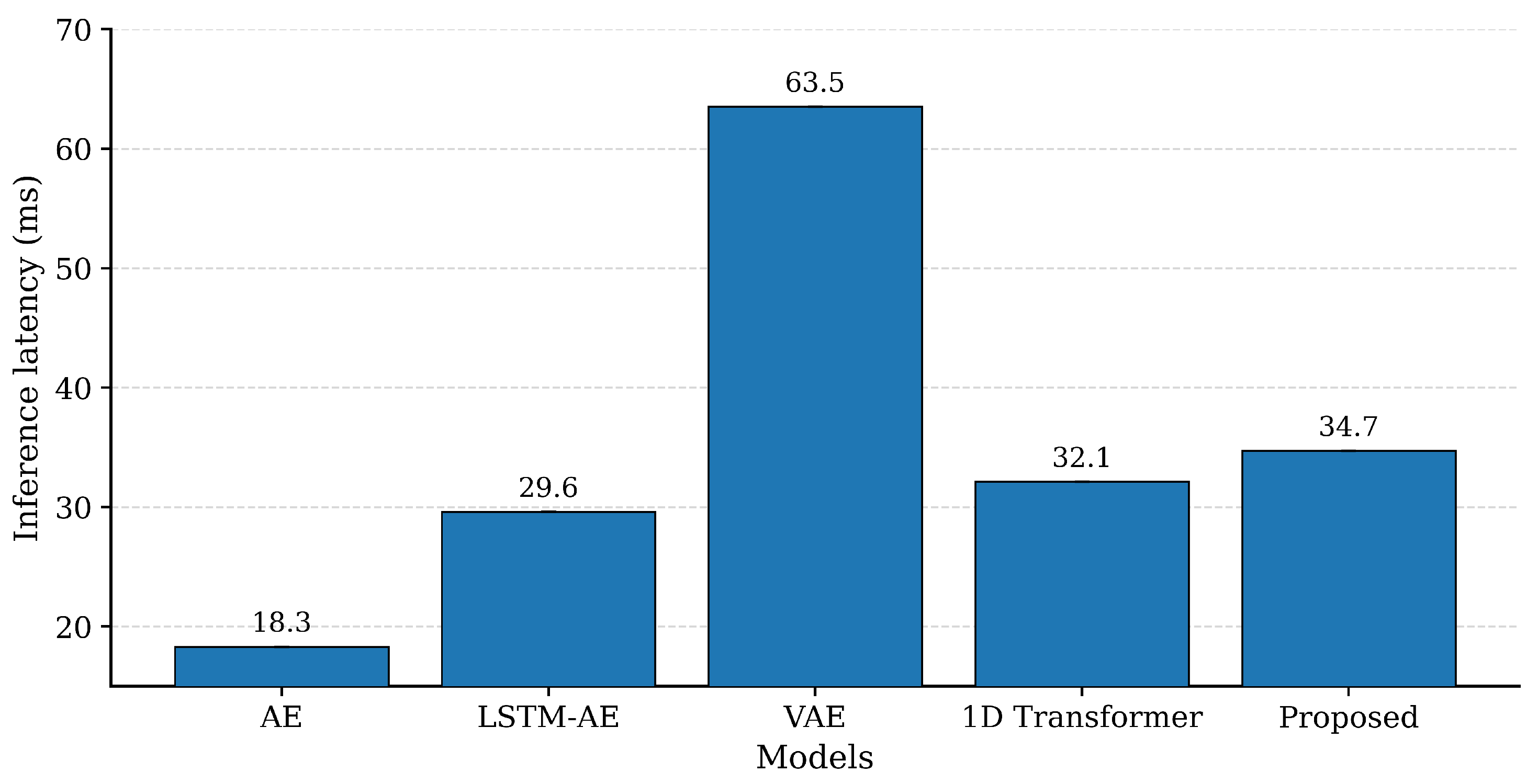
Inference latency comparison across models.
Figure 18.
Inference latency comparison across models.
Table 1.
Summary of dataset and sliding window statistics.
Table 1.
Summary of dataset and sliding window statistics.
| Item | Value |
|---|
| Total number of frames | ≈1.2 |
| Number of features per frame (d) | 6 |
| Anomalous frames ratio | <1% |
| Flight/session duration | ≈2000 flight hours |
| Train/Validation/Test split | 60%/20%/20% |
| Sliding window length (T) | 32 frames |
| Sliding window stride (s) | 8 frames |
| LKRP embedding dimension (m) | 50 |
| DMR retained components (p) | 20 |
Table 2.
Composition of operational vs. simulated anomalies.
Table 2.
Composition of operational vs. simulated anomalies.
| Split | Operational Anomalies | Simulated Anomalies | Notes |
|---|
| Training | ≈20% | ≈80% | used for model training |
| Validation | | | real anomalies only |
| Test | | | real anomalies only |
Table 3.
Overall performance comparison of anomaly detection methods (mean ± std over 5 runs). Bold values indicate the best performance across all methods.
Table 3.
Overall performance comparison of anomaly detection methods (mean ± std over 5 runs). Bold values indicate the best performance across all methods.
| Method | Acc | Prec. | Rec. | F1 | AUC |
|---|
| SVM (RBF) | | | | | |
| Random Forest | | | | | |
| PCA–LR | | | | | |
| Autoencoder | | | | | |
| LSTM–AE | | | | | |
| VAE | | | | | |
| Proposed | | | | | |
Table 4.
Comparison of imbalance mitigation strategies using the same CNN–LSTM detector (mean ± std over 5 runs). Bold values indicate the best performance among all strategies.
Table 4.
Comparison of imbalance mitigation strategies using the same CNN–LSTM detector (mean ± std over 5 runs). Bold values indicate the best performance among all strategies.
| Training Strategy | Precision | Recall | F1 | AUC |
|---|
| No augmentation | | | | |
| Class-weighted BCE | | | | |
| SMOTE oversampling | | | | |
| WGAN-GP augmentation | | | | |
| Proposed CT–WGAN | | | | |
Table 5.
Generalization to unseen anomaly scenarios (F1-score). Bold values indicate the overall average performance across unseen anomaly types.
Table 5.
Generalization to unseen anomaly scenarios (F1-score). Bold values indicate the overall average performance across unseen anomaly types.
| Unseen Anomaly Type | F1-Score |
|---|
| Multipath interference | |
| Electromagnetic interference | |
| Hardware degradation | |
| Average | |
Table 6.
Robustness to noisy condition vectors.
Table 6.
Robustness to noisy condition vectors.
| Condition Perturbation | F1-Score |
|---|
| No noise | |
| Gaussian noise () | |
| Gaussian noise () | |
| Missing 20% conditions | |
| Missing 40% conditions | |
Table 7.
Ablation study results (mean ± standard deviation over five runs).
Table 7.
Ablation study results (mean ± standard deviation over five runs).
| Configuration | F1 | AUC |
|---|
| Full Model (LKRP + DMR + CT–WGAN) | | |
| Without CT–WGAN | | |
| Without DMR | | |
| Without LKRP | | |
| CNN–LSTM Raw | | |
Table 8.
Computational complexity and real-time latency comparison across models. Bold values indicate the proposed method.
Table 8.
Computational complexity and real-time latency comparison across models. Bold values indicate the proposed method.
| Model | Params (M) | FLOPs (M) | Latency (ms) | Meets 100 ms? |
|---|
| Autoencoder (AE) | 0.42 | 0.51 | 18.3 | Yes |
| LSTM–AE | 0.78 | 1.21 | 29.6 | Yes |
| VAE | 1.12 | 1.79 | 41.2 | Yes |
| 1D Transformer | 1.85 | 3.46 | 63.5 | Yes |
| CNN–LSTM (raw) | 0.65 | 0.74 | 32.1 | Yes |
| Proposed | 0.69 | 0.71 | 34.7 | Yes |