A Non-Iterative Calculation Method for Zero-Dimensional Nozzle Model of Gas Turbine Engine

Abstract

To address the real-time performance issue of the zero-dimensional nozzle model for gas turbine engines, a non-iterative computational method is proposed that determines the flow regime (subcritical vs. choked) via characteristic Mach number and characteristic flow factor. This method eliminates iterative solution procedures, thereby reducing computational time, and solves the problem of discontinuous throat mass flow rate calculation at the transition flow regime from subcritical to choked in traditional nozzle models. The method is applied to improve a component-level turbofan engine model and is validated through numerical simulation. Simulation results indicate that, compared with traditional nozzle models requiring two and eight iterations, the non-iterative nozzle model reduces computation time by $69.7\%$ and $85.71\%$, respectively. The turbofan engine model incorporating the non-iterative nozzle model achieves a 24.58% reduction in maximum per-step computation time and a 13.7% reduction in average per-step computation time compared with the traditional model, while maintaining comparable simulation accuracy. The proposed method substantially enhances the real-time simulation performance of the component-level turbofan engine model, and can be readily extended to other component-level models—whether based on iterative-solution schemes or on volume-based modeling approaches.

1. Introduction

With the increasing trend toward intelligent and autonomous development of aero-engine propulsion systems, Component-Level Models (CLM), owing to their high fidelity and interpretability, have been widely applied in engine health management, control system design, and flight simulation.

However, traditional CLMs face significant bottlenecks in real-time performance, making it difficult for on-board control systems and online diagnostics to meet stringent requirements for both rapid response and reliability. As a result, enhancing the real-time computational capability of CLMs while maintaining model accuracy has become a key research challenge in recent years [1,2,3,4,5,6].

In terms of iterative algorithms, Wang et al. proposed a hybrid damping Newton method based on Non-dominated Sorting Differential Evolution (NSDE) to improve the convergence of Newton iterations in CLMs. This approach significantly enhances real-time computational performance under large-deviation conditions. Numerical simulations demonstrated that the maximum deviation from experimental reference values was limited to 8.1% [7]. Lu et al. proposed an improved iterative scheme that reuses the Jacobian matrix over multiple steps to reduce the computational cost of Jacobian evaluations, without sacrificing model accuracy [8]. Stamatis et al. introduced a five-step fixed-point iteration method into adaptive engine models, achieving faster-than-real-time performance even on low-power processors, while maintaining simulation steady-state errors below 1% [9]. In addition, several non-iterative approaches have been developed by introducing complementary variables and equations from engine volumetric dynamics to close the nonlinear system algebraically, enabling direct solution without iteration [10,11,12,13], while these methods enhance solution stability, their reliance on small time steps limits improvements in overall real-time performance.

In terms of data processing and interpolation, Cai et al. developed a fast interpolation method based on the maximum parameter slope to automatically determine the interpolation cut in point. Compared with traditional sequential interpolation techniques, this approach improved characteristic interpolation efficiency by 47.5% and reduced the total flow path computation time by 74.3% [14]. Yin et al. significantly improved the real-time performance of CLMs by constructing interpolation tables for gas thermodynamic properties. This approach reduced the flow path computation time to as low as 0.02 ms on a 3.3 GHz platform, while maintaining simulation accuracy [15]. Chen et al. proposed a fast turbine characteristic computation method based on time complexity analysis. The method achieves both high accuracy and real-time performance, with a 3.04-fold increase in computing speed [16]. Zheng et al. employed a neural-network-assisted Newton–Raphson method for computing working medium thermodynamic properties. Compared with fixed-initial-value iteration, this approach significantly reduced the number of iterations, cutting the computation time of thermodynamic parameters by up to 47% [17]. Ren et al. propose a thermodynamic-based and data-driven hybrid model for aero-engine degradation evaluation. Different from thermodynamic-based methods, the iteration calculation is converted to the forward flow in the proposed neural network, thus improving convergence [18].

In terms of system-level integration and optimization of component algorithms, Chen et al. proposed an adaptive composite model based on CLM, State-Space Model (SSM), and Kalman Filter (KF), enabling the Nonlinear Model Predictive Controller (NMPC) to compute the CLM only once at each sampling instant, thereby outperforming traditional NMPC in both response speed and real-time performance [19]. Mihaloew et al. developed a hybrid model by combining real and pseudo dynamics, achieving a single-step computation time of 2.0 ms on a Univac 1110 computer and 5.7 ms on the simulator computer (Xerox Sigma 8) [20]. Liu et al. effectively resolved the conflict between computational speed and accuracy in the real-time simulation of a twin-spool turbojet engine by employing software-level design strategies such as macro assembly programming and parallel floating-point computation [21]. Sui et al. achieved a dynamic balance between accuracy and computational speed by integrating non-real-time and real-time models [22]. Li et al. improved the convergence and real-time performance of the actuator model within a 20 ms simulation cycle by tuning the parameters of a fixed-step algorithm [23]. Zheng et al. introduced the Feasible-One-Pass Newton method to enable efficient computation under high-dimensional coupling for integrated inlet-engine modeling, achieving efficient solutions across the full flight envelope [24]. Zheng et al. integrated the CLM with a compact propulsion system dynamic model and enhanced both steady-state and dynamic accuracy through online feedback correction, achieving significantly better real-time performance compared to traditional CLM approaches [25]. Zong et al. proposed a component-level identification modeling method based on the Hammerstein system, in which each engine component is treated as a Hammerstein system—comprising a static nonlinear part followed by a dynamic linear part. Using system identification techniques, the model captures both the dynamic linear and static nonlinear characteristics of each component. The method achieved an average relative error below 4% and significantly reduced computation time [26].

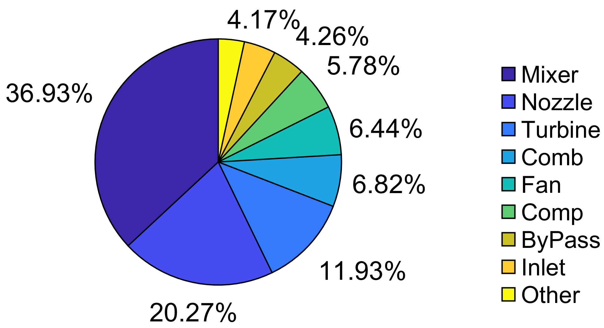
To further enhance the real-time performance and numerical convergence of the CLM, this study uses the Intel VTune Profiler software 2025.5.0 to analyze the computational time distribution of a component-level turbofan engine model, as illustrated in Figure 1. Among all components, the mixer and nozzle modules exhibit the highest computational cost. This is primarily because, in both modules, the Mach number must be implicitly calculated through the flow factor, which involves iterative solutions of transcendental equations and therefore consumes substantial computational time.

To address the high computational cost associated with the aerodynamic and thermodynamic calculations of the nozzle model, this study evaluates the traditional nozzle model and proposes a novel performance calculation method for the nozzle model. The proposed approach enables direct determination of the throat mass flow rate without iterative computation, significantly reducing the computational time. Unlike previous studies that focused on iterative algorithms, data processing and interpolation, and system-level integration and optimization of component algorithms, this study delves into the underlying aerodynamic and thermodynamic formulas of the model, optimizing the formulas themselves to achieve faster computation while maintaining accuracy. Moreover, the modifications introduced in this study operate on a different dimension than existing optimization methods, allowing them to work synergistically with other strategies and be directly applied to any component-level engine model. In this study, the method is applied to improve a turbofan engine CLM, and numerical simulations are conducted to validate its performance.

2. Traditional Nozzle Model

The present study focuses on the nozzle model within an aero-engine component-level zero-dimensional model. This model simplifies all nozzle types into an ideal nozzle characterized by a throat (the location of the minimum cross-sectional area) and an exit (the location of the terminal cross-section of the nozzle). For a purely convergent nozzle, the throat and exit coincide. Furthermore, the model assumes adiabatic and isentropic flow, neglecting any total pressure loss or heat exchange with the nozzle walls.

In the iterative solution process of the CLM, the nozzle computation procedure is as follows: based on the available pressure drop across the nozzle, the throat mass flow rate $W_t$ is calculated and compared with the inlet mass flow rate $W_i$ obtained from the upstream component. The difference between $W_t$ and $W_i$ defines the mass flow residual $ϵ$, which serves as the convergence criterion in the CLM iterative process.

In the CLM, the residual represents the degree to which the current solution fails to satisfy the various balance equations, such as mass flow balance, static pressure balance, and power balance, that couple adjacent components in the engine’s gas path. It quantitatively reflects the deviation from the physical balance conditions required for a consistent steady-state solution. Only when these residuals are reduced below prescribed tolerance thresholds can the overall engine model be considered physically consistent and numerically converged, making residual magnitude a core criterion for judging whether the solution has successfully converged.

Because the engine system is highly nonlinear and strongly coupled across components, solving these balance equations requires iterative numerical methods that adjust unknown variables to progressively reduce all residuals. In each iteration, the flow conditions, pressure states, and corresponding residuals of each component must be repeatedly recalculated, and these repeated residual evaluations drive the update of the solution variables until convergence is achieved. This necessitates computing the residuals multiple times at each iteration. Therefore, in the iterative process of the CLM, the computation of the nozzle model is, in essence, aimed at determining the residuals $ϵ$.

2.1. Traditional CalculationMethod for Residual of Mass Flow Rate

The Mach number at the nozzle throat $M_t$ rises with the available pressure drop until the flow becomes choked $(M_t=1)$. When $M_t<1$, the nozzle is in a subsonic flow regime, whereas when $M_t=1$, the flow becomes choked. The mass flow through the nozzle throat is evaluated differently depending on whether the nozzle is subsonic or choked; therefore, the flow regime must be identified first.

In the traditional nozzle model, the flow regime is determined on the basis of a characteristic pressure, denoted as ${{p_s}_e}_1$. This quantity is not the actual static pressure at the nozzle exit; rather, it represents the back pressure that would exist at the exit section under the assumed flow condition—namely, a choked throat $(M_t=1)$ followed by entirely subsonic flow in the divergent section. In other words, ${{p_s}_e}_1$ is the back pressure that satisfies the assumed flow condition. Only after its value is obtained is the ambient static pressure ${p_s}_0$ compared with ${{p_s}_e}_1$ to determine the actual flow regime and to subsequently calculate the throat mass flow factor $q_t$. Finally, the throat mass flow rate $W_t$ and the mass flow rate residual $ϵ$ are calculated. The detailed procedure is outlined below, where the formulas can be found in Refs. [27,28].

1.

The nozzle exit Mach number ${M_e}_1$, under the assumption of a choked throat and subsonic flow in the divergent section, is determined using the mass flow factor equation:

$${\displaystyle \frac{A_t}{A_e}}={M_e}_1{\left[{\displaystyle \frac{2}{k+1}}(1+{\displaystyle \frac{k-1}{2}}{{M_e}_1}^2)\right]}^{-{\displaystyle \frac{k+1}{2(k-1)}}}$$

(1)

where $A_e$ is the nozzle exit area; $A_t$ is the throat area (the minimum cross-sectional area of the nozzle); for a converging nozzle, $A_t=A_e$; k is the isentropic exponent.

In practical computations, this equation generally yields two solutions for ${M_e}_1$. Since the assumed flow regime in the divergent section is subsonic, the solution satisfying ${M_e}_1<1$ is chosen. As this equation is a transcendental equation in terms of ${M_e}_1$, it cannot be solved analytically and typically requires iterative numerical methods.

2.

The ${{p_s}_e}_1$ can be determined from ${M_e}_1$ as follows:

$${{p_s}_e}_1=p_i{(1+{\displaystyle \frac{k-1}{2}}{{M_e}_1}^2)}^{-{\displaystyle \frac{k}{k-1}}}$$

(2)

where $p_i$ is the total pressure at the nozzle inlet.

3.

The actual flow regime is determined by comparing ${{p_s}_e}_1$ with ${p_s}_0$, and the $q_t$ is then determined as follows:

$$q_t=\left\{\begin{array}{cc}{\displaystyle \frac{A_e}{A_t}}{M}_e{\left[{\displaystyle \frac{2}{k+1}}(1+{\displaystyle \frac{k-1}{2}}{M_e}^2)\right]}^{-{\displaystyle \frac{k+1}{2(k-1)}}}\hfill & {{p_s}_e}_1<{p_s}_0\left(\mathrm{subcritical}\right)\hfill \\ 1\hfill & {{p_s}_e}_1\ge {p_s}_0\left(\mathrm{choked}\right)\hfill \end{array}\right.$$

(3)

where $q_t$ is the nozzle throat mass flow factor; $M_e$ is the nozzle exit Mach number under the subcritical flow regime, given by the following: $M_e=\sqrt{{\displaystyle \frac{2}{k-1}}[{\left({\displaystyle \frac{{p_s}_0}{p_i}}\right)}^{{\displaystyle \frac{1-k}{k}}}-1]}$.

4.

The $W_t$ can be determined from $q_t$ as follows:

$$W_t=A_t\sqrt{{\displaystyle \frac{k}{R{T}_i}}{\left({\displaystyle \frac{2}{k+1}}\right)}^{{\displaystyle \frac{k+1}{k-1}}}}{p}_i{q}_t$$

(4)

where $W_t$ is the nozzle throat mass flow rate; R is the specific gas constant; $T_i$ is the total temperature at nozzle inlet.

5.

The $ϵ$ can be determined as follows:

$$ϵ={\displaystyle \frac{W_t}{W_i}}-1$$

(5)

where $ϵ$ represents the flow residual and serves as one of the iteration residuals in the component-level model (CLM).

2.2. Simulation and Analysis of Traditional Nozzle Model

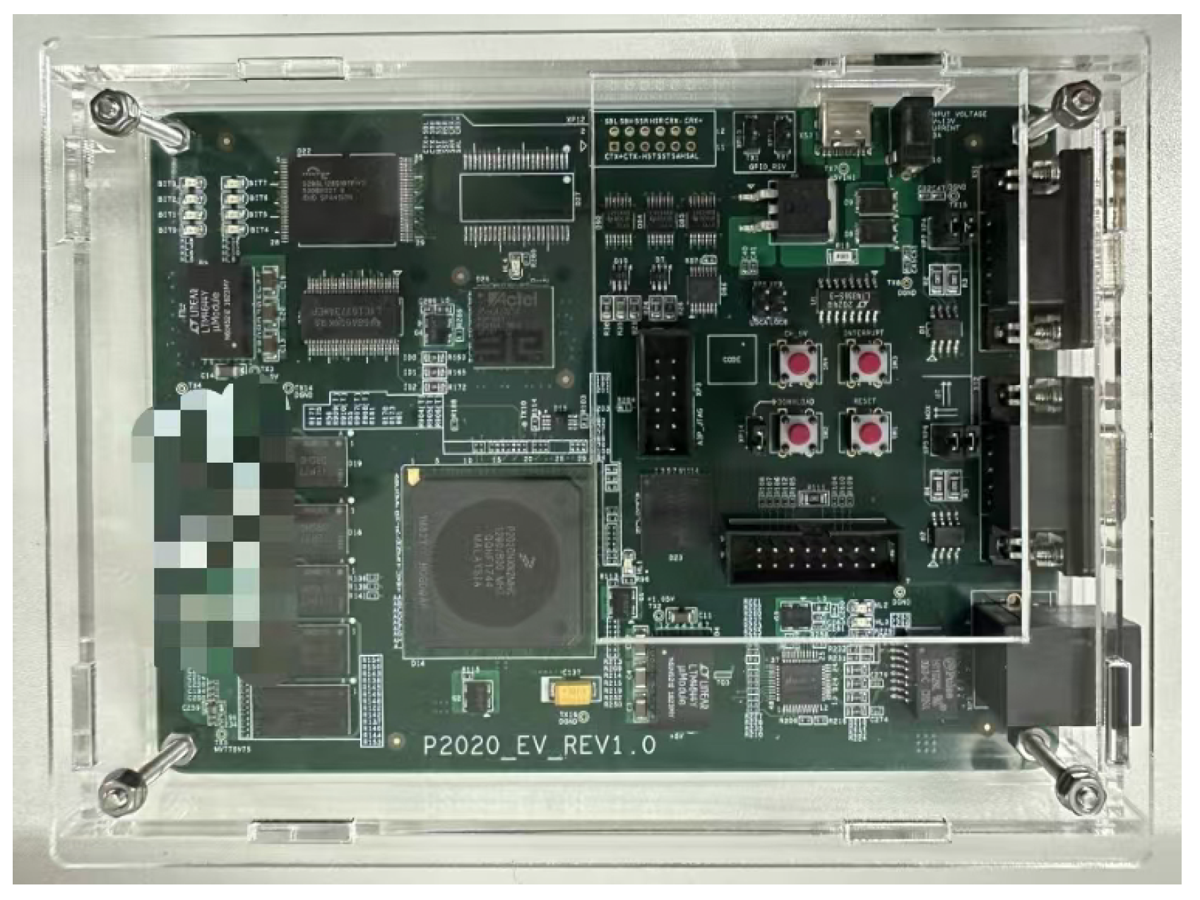
To evaluate the computational performance of the traditional nozzle model, numerical tests were conducted on a PowerPC P2020 (sourced from Freescale, Tempe, AZ, USA) processor platform (operating frequency: 1.2 GHz), which is commonly used in embedded control systems for aerospace and industrial equipment. A photograph of the platform is provided in Figure 2. The computational time of basic operations, measured using 32-bit single-precision data on this platform, is summarized in

Table 1. Computational Time of Basic Operations in P2020 Processor Platform.

Operation Type	Symbol	Computational Time (ns)	Relative Time
Addition	+	3151	1
Subtraction	−	3353	1.06
Multiplication	*	3302	1.05
Division	/	4201	1.33
Exponentiation	⌃	31,250	9.92

.

An analysis of the computational procedure of the traditional nozzle model was conducted to determine the number of basic operations and the relative time associated with each step, as summarized in

Table 2. Operation Count of Traditional Nozzle Model.

Steps	+	−	*	/	⌃	Relative Time
1	3	2	5	3	1	$24.29n$
2	4	6	6	6	2	44.51
3	3	5	7	7	3	54.75
4	2	1	5	3	2	32.14
5	0	1	0	1	0	2.40
Sum	12	15	22	20	8	$133.8+24.29n$

. Considering that the first step involves n iterative cycles, the total relative time per evaluation can be approximated by $133.8+24.29n$.

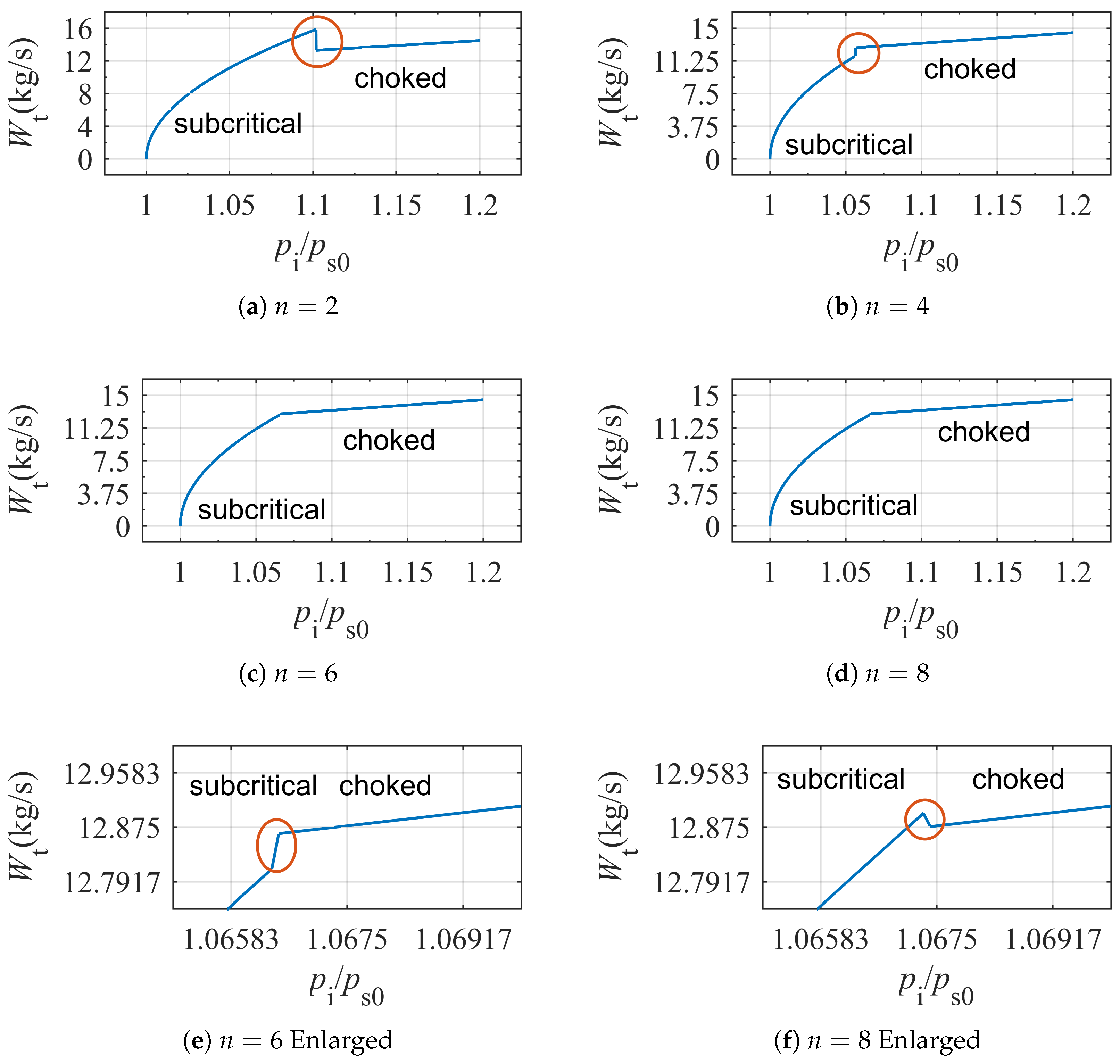
Figure 3 presents the relationship between the $W_t$ and the $p_i/{p_s}_0$ for the traditional nozzle model, where Equation (1) is iteratively solved using the bisection method under the conditions $A_t=0.05{\mathrm{m}}^2$, $A_e=0.1{\mathrm{m}}^2$, $T_i=300\mathrm{K}$, $k=1.4$, and ${p_s}_0$ = 101,325 Pa, with different iteration numbers n. The $p_i/{p_s}_0$ is varied linearly from 1.0 to 1.2 with a simulation step size of ${10}^{-6}$. The total computational time corresponding to these conditions is summarized in

Table 3. Traditional Nozzle Model Computational Time.

n	2	4	6	8
Computational Time (ms)	165	216	274	351

.

It can be observed that the $W_t$ generally increases monotonically with the $p_i/{p_s}_0$ in the results obtained using the traditional nozzle model. As the number of iterations n increases, the resulting flow curve becomes closer to a smooth, monotonically increasing curve, i.e., the accurate $W_t$ curve.

However, since the traditional nozzle model obtains only an approximate numerical solution through iterative computation, the calculated $W_t$ curve exhibits discontinuities or even non-monotonic behavior near the subcritical-to-choked transition flow regime, regardless of the iteration number (as highlighted by the red circle in the figure). This, in turn, induces a discontinuity in the total engine CLM near the corresponding operating condition.

To ensure convergence of the Newton–Raphson iterative process when solving the co-operating equations in total engine CLMs, it is imperative that the first derivatives of co-operating equations satisfy the following conditions:

1.

The first derivative must be continuous in the vicinity of the solution;

2.

The first derivative must exist and be non-zero.

Consequently, the discontinuity of the total engine CLM near this operating condition compromises model convergence, causing the Newton–Raphson iterative process to oscillate or diverge. Although increasing the number of iterations in Equation (1) can partially mitigate the issue, it compromises the real-time performance of the total engine CLM.

3. Non-Iterative Nozzle Model

To improve the real-time performance of the nozzle model and the accuracy near the subcritical-to-choked transition flow regime, this study proposes a non-iterative nozzle model.

Analysis of the $W_t$ curves in Figure 3, reveals the curve consists of two curves: the subcritical and choked curve, with the transition point at their intersection.

Based on the calculation method of the traditional nozzle model, the analytical expressions for these two curves can be derived as follows:

$$W_t=\left\{\begin{array}{cc}{A}_e{p_s}_0\sqrt{{\displaystyle \frac{2k}{(k-1)R{T}_i}}}{\left({\displaystyle \frac{p_i}{{p_s}_0}}\right)}^{{\displaystyle \frac{k-1}{2k}}}\sqrt{{\left({\displaystyle \frac{p_i}{{p_s}_0}}\right)}^{{\displaystyle \frac{k-1}{k}}}-1}\hfill & \left(\mathrm{subcritical}\right)\hfill \\ A_t{p_s}_0\sqrt{{\displaystyle \frac{k}{R{T}_i}}{\left({\displaystyle \frac{2}{k+1}}\right)}^{{\displaystyle \frac{k+1}{k-1}}}}{\displaystyle \frac{p_i}{{p_s}_0}}\hfill & \left(\mathrm{choked}\right)\hfill \end{array}\right.$$

(6)

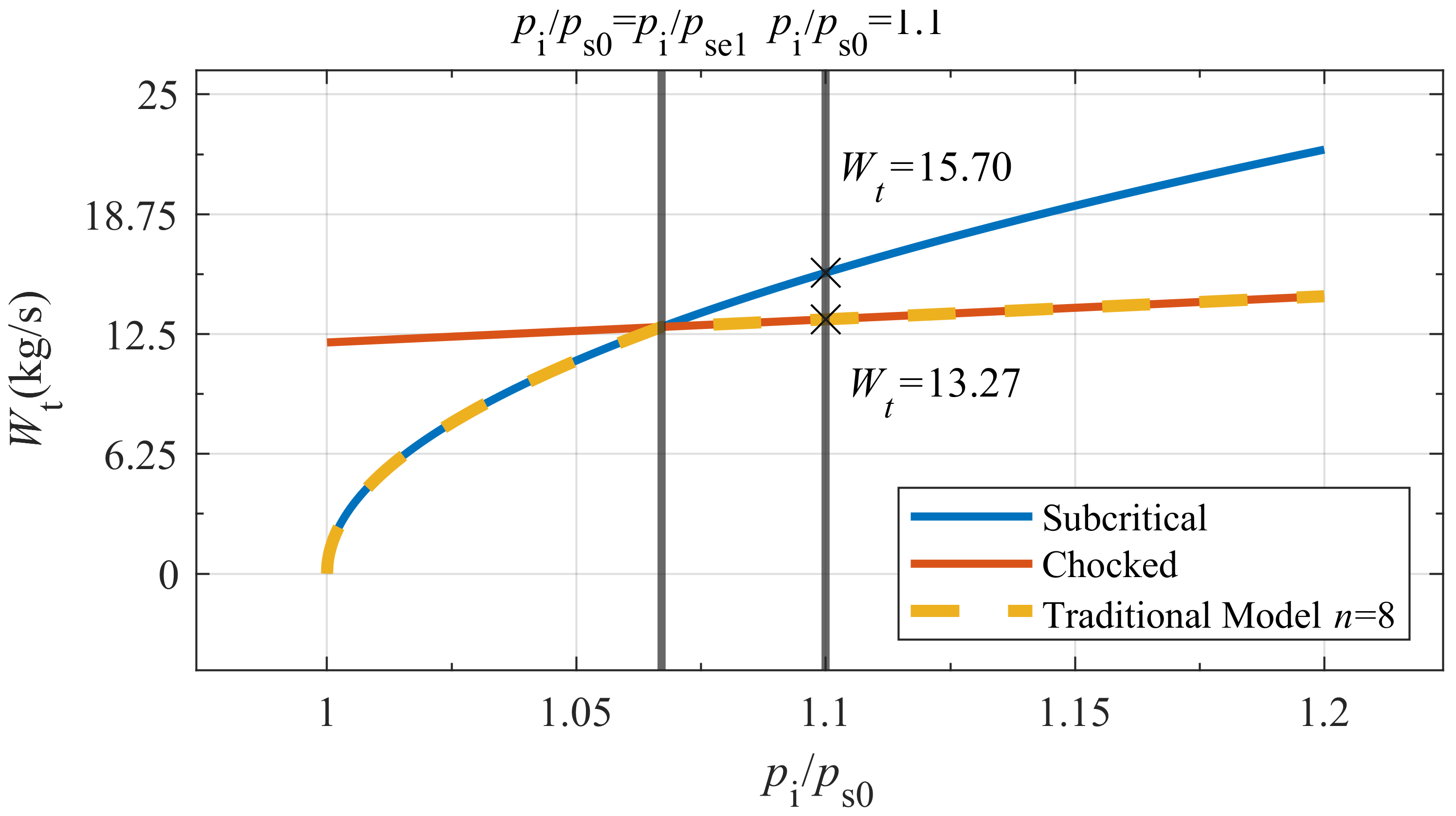
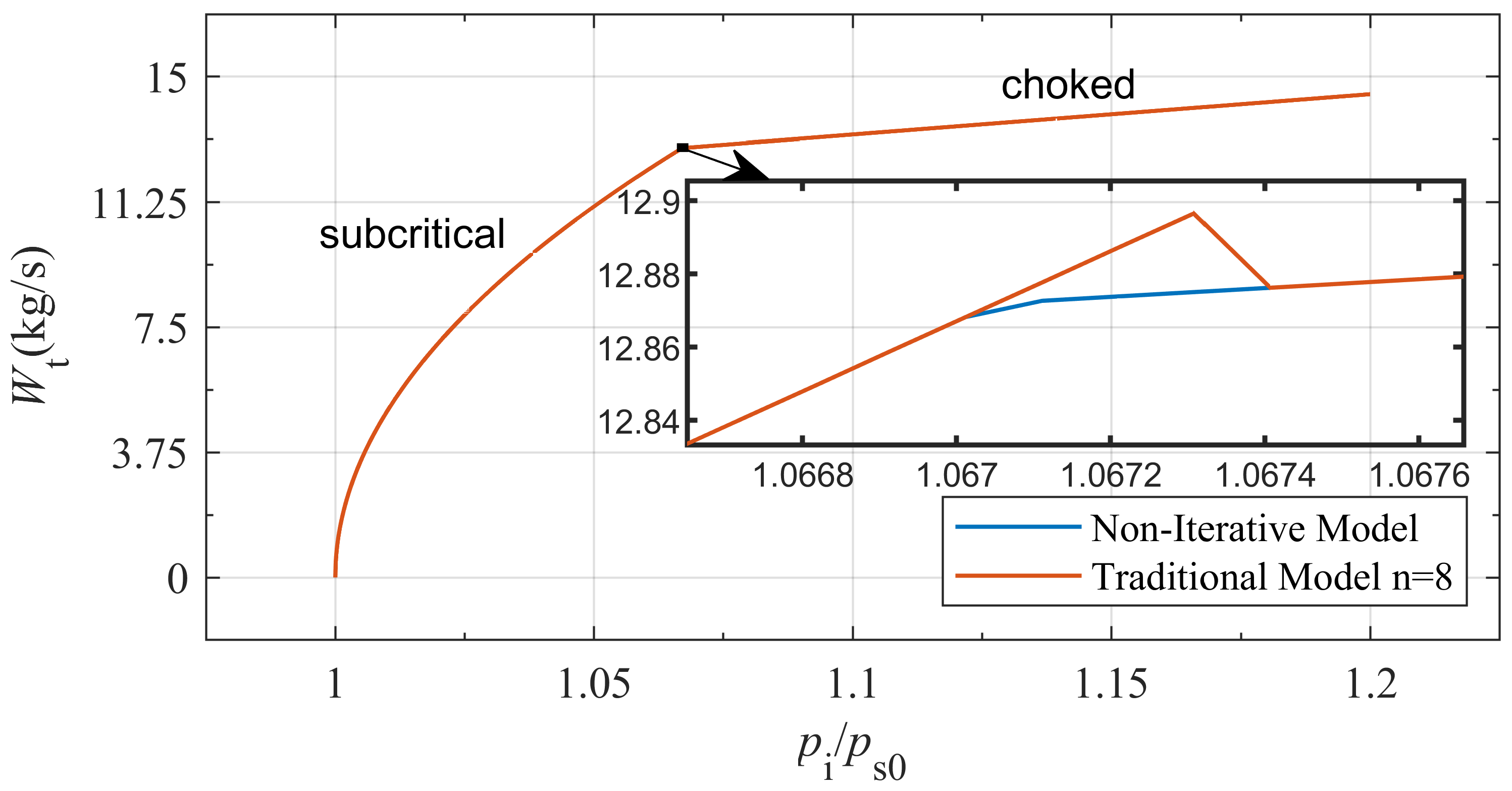
Figure 4 presents the subcritical and choked curves for $A_t=0.05{\mathrm{m}}^2$, $A_e=0.1{\mathrm{m}}^2$, $T_i=300\mathrm{K}$, $k=1.4$, and ${p_s}_0$ = 101,325 Pa. The functional forms of the subcritical and choked curves are given by Equation (6). The $W_t$ curve obtained from 8 iterations of the traditional nozzle model (Traditional Model n = 8) almost coincides with the piece-wise curve formed by connecting the subcritical and choked curves at their intersection.

As shown in Figure 4, traditional nozzle models determine the flow regime by iteratively computing the intersection $p_i/{{p_s}_e}_1$ and comparing it with the actual $p_i/{p_s}_0$ to establish whether it lies to the left or right of the intersection—i.e., whether the nozzle operates in a subcritical or choked flow regime.

However, two $W_t$ can also be directly calculated from the subcritical and choked curves for a given $p_i/{p_s}_0$, with the flow regime determined by the smaller value. As shown in Figure 4, for $p_i/{p_s}_0=1.1$, the subcritical curve gives $W_t=15.7\mathrm{kg}/\mathrm{s}$, while the choked curve gives $W_t=13.27\mathrm{kg}/\mathrm{s}$. Since the choked $W_t$ is smaller, the nozzle is in the choked flow regime, and the actual $W_t$ corresponds to the choked $W_t$. Both $W_t$ values can be obtained directly from Equation (6), without iteration.

By refining and assigning physical meaning to each step of the above method, the final non-iterative nozzle model is formulated as follows.

3.1. Non-Iterative Calculation Method for Residual of Mass Flow Rate

In the non-iterative nozzle model, the flow regime is determined based on the characteristic Mach number ${M_e}_1$ and the characteristic flow factor ${q_t}_1$. The core procedure is as follows. First, the subcritical flow regime is assumed. Under this assumption, the exit Mach number ${M_e}_1$ and the throat flow factor ${q_t}_1$ are computed as the characteristic parameter. Comparing these values with 1 identifies the actual flow regime, from which the actual throat mass flow factor, $q_t$, is obtained. Finally, the throat mass flow rate $W_t$, and the residual mass flow rate $ϵ$, are calculated. The detailed procedure is outlined below:

1.

The ${M_e}_1$ can be determined from $p_i/{p_s}_0$ as:

$${M_e}_1=\sqrt{{\displaystyle \frac{2}{k-1}}[{\left({\displaystyle \frac{p_i}{{p_s}_0}}\right)}^{{\displaystyle \frac{k-1}{k}}}-1]}$$

(7)

2.

The ${q_t}_1$ can be determined from ${M_e}_1$ as:

$${q_t}_1={\displaystyle \frac{A_e}{A_t}}{M_e}_1{\left[{\displaystyle \frac{2}{k+1}}(1+{\displaystyle \frac{k-1}{2}}{{M_e}_1}^2)\right]}^{{\displaystyle \frac{k+1}{2(1-k)}}}$$

(8)

3.

The actual flow regime is determined by ${M_e}_1$ and ${q_t}_1$, and the $q_t$ is then determined as:

$$q_t=\left\{\begin{array}{cc}{q_t}_1\hfill & {q_t}_1\le 1\mathrm{AND}{M_e}_1\le 1\left(\mathrm{subcritical}\right)\hfill \\ 1\hfill & \mathrm{ELSE}\left(\mathrm{choked}\right)\hfill \end{array}\right.$$

(9)

4.

The $W_t$ can be determined from $q_t$ as:

$$W_t=A_{thr}\sqrt{{\displaystyle \frac{k}{R{T}_i}}{\left({\displaystyle \frac{2}{k+1}}\right)}^{{\displaystyle \frac{k+1}{k-1}}}}{p}_i{q}_t$$

(10)

5.

The $ϵ$ can be determined as:

$$ϵ={\displaystyle \frac{W_t}{W_i}}-1$$

(11)

Compared with the traditional nozzle model, the non-iterative model provides exact values of $W_t$ and $ϵ$ without iteration. Each computational step directly contributes to the flow residual, eliminating redundant calculations. Consequently, this method represents the most streamlined approach for computing the nozzle flow residual $ϵ$.

3.2. Simulation and Analysis of Non-Iterative Nozzle Model

An analysis of the computational procedure of the improved nozzle model was conducted to determine the number of basic operations and the relative time associated with each step, as summarized in

Table 4. Operation count of the non-iterative nozzle model.

Steps	+	−	*	/	⌃	Relative Time
1	0	3	1	3	2	28.08
2	3	1	5	4	1	24.56
3	0	0	0	0	0	0
4	1	0	4	4	2	30.37
5	0	1	0	1	0	2.40
Sum	4	5	10	12	5	85.40

. The total relative time per evaluation can be approximated by $85.40$, which is only about $54\%$ of the relative time required for a single iteration of the traditional model.

Figure 5 presents the relationship between the $W_t$ and the $p_i/{p_s}_0$ for the non-iterative nozzle model, under the conditions $A_t=0.05{\mathrm{m}}^2$, $A_e=0.1{\mathrm{m}}^2$, $T_i=300\mathrm{K}$, $k=1.4$, and ${p_s}_0$ = 101,325 Pa. The $p_i/{p_s}_0$ is varied linearly from 1.0 to 1.2 with a simulation step size of ${10}^{-6}$. The total computation time is $10\mathrm{ms}$. The $W_t$ curve predicted by the non-iterative nozzle model closely aligns with that of the traditional model using 8 iterations, remaining monotonic and continuous across the subcritical-to-choked flow transition. The non-iterative approach decreases computational time by 69.7% and 85.71% compared with the traditional model using two and eight iterations, respectively.

4. Simulation and Analysis of Nozzle Non-Iterative Turbofan Engine Model

To assess the impact of the non-iterative nozzle model on CLM performance, it was integrated into a turbofan CLM. Dynamic simulations were performed on the P2020 and the Xeon8280 Processor (sourced from Intel, Santa Clara, CA, USA) platform for engine operation under idle to maximum conditions at ground level.

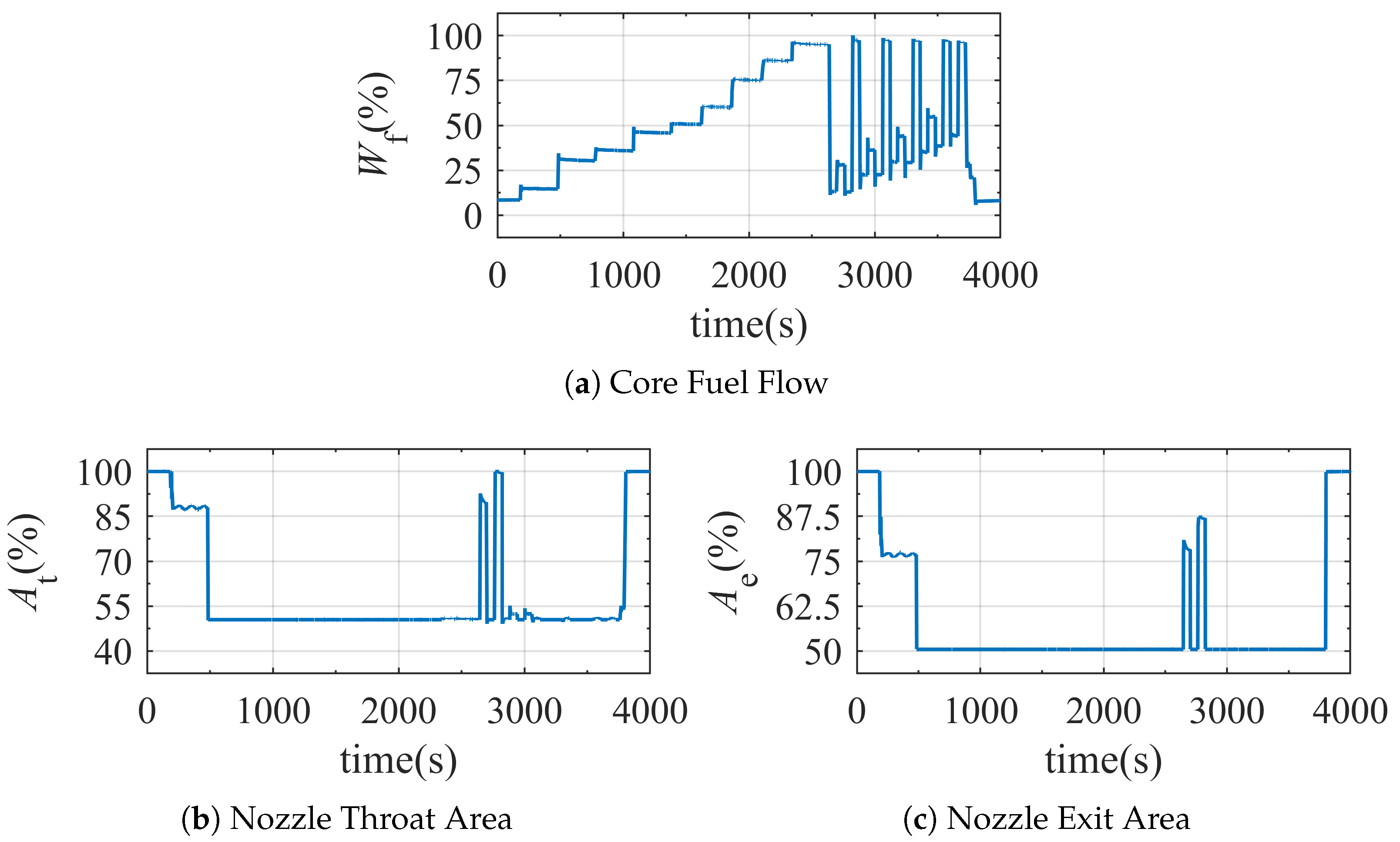
Control inputs are provided in Figure 6. Subfigures (a), (b), and (c) depict the time-dependent variations of the main fuel flow rate ($W_f$), nozzle throat area ($A_t$), and nozzle exit area ($A_e$), respectively. The period from 0 to 2500 s corresponds to steady-state tests, while the period from 2500 to 4000 s corresponds to transient tests involving acceleration and deceleration.

Simulations were run for a total duration of $t=4000\mathrm{s}$ with a time step of $\Delta t=25\mathrm{ms}$.

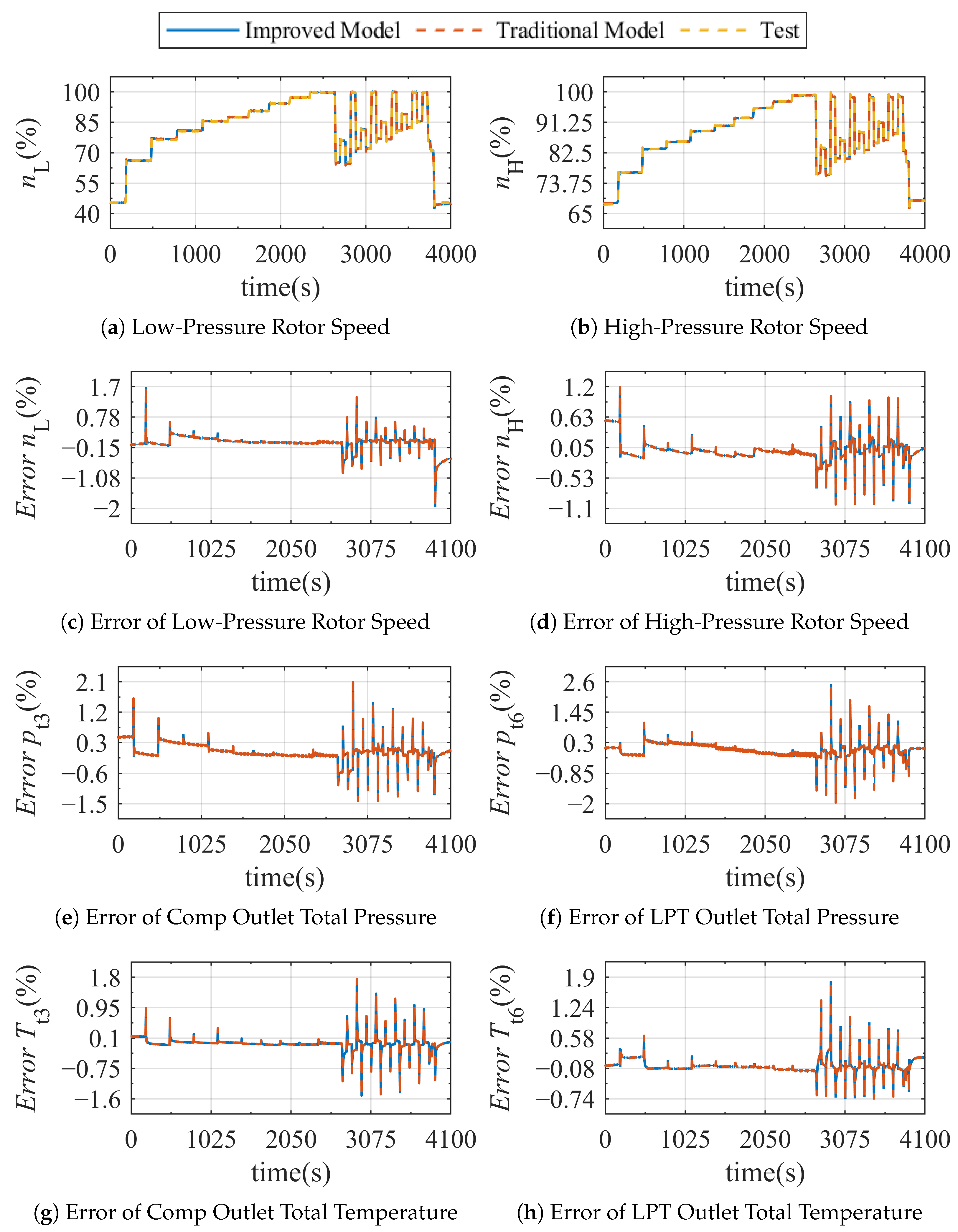
Time-varying model simulation error curves for spool speed and key parameters, comparing the improved and traditional turbofan CLMs, are presented in Figure 7. Subfigures (a) and (b) depict the time-dependent variations of the low-pressure spool speed ($n_L$) and high-pressure spool speed ($n_H$), respectively. Subfigures (c) to (h) depict the time-dependent variations of the model simulation error for low-pressure spool speed ($Error{n}_L$), high-pressure spool speed ($Error{n}_H$), compressor exit total pressure ($Error{p}_3$), turbine exit total pressure ($Error{p}_6$), compressor exit total temperature ($Error{T}_3$), and turbine exit total temperature ($Error{T}_6$), respectively. The model simulation error is defined as:

$$Error={\displaystyle \frac{dat{a}_{Sim}}{dat{a}_{Test}}}-1$$

(12)

where $dat{a}_{Sim}$ is the model calculation result; $dat{a}_{Test}$ is the test measurement result.

As shown in Figure 7, larger computational errors are observed during the transient acceleration and deceleration phase from 2500 to 4000 s. This is primarily because the throttle lever is rapidly pushed up and pulled down around this time, causing drastic changes in the engine state. Since most component characteristics are based on steady-state tests, in which the transition process is assumed to occur instantaneously, the model neglects the actual flow inertia and hysteresis effects. In addition, other modeling factors, such as errors in the rotor rotational inertia and variations in turbine blade tip clearance, further increase the parameter errors in both the traditional and the improved models during this transient state.

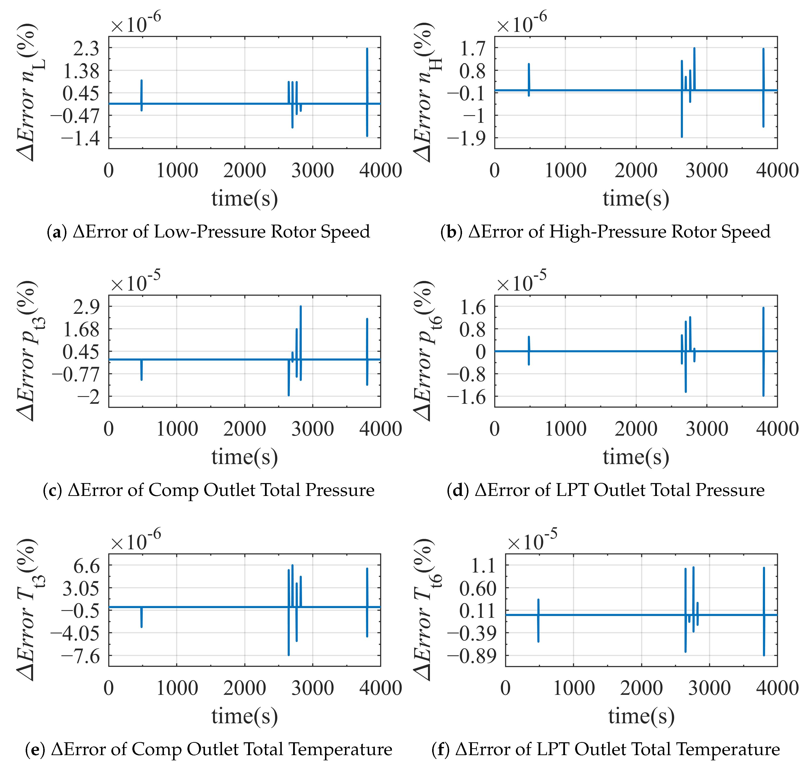
Time-varying differences model simulation error between the traditional and improved turbofan CLM curves for spool speed and key parameters are presented in Figure 8. Subfigures (a) to (f) depict the time-dependent variations of the differences model simulation error for low-pressure spool speed ($\Delta Error{n}_L$), high-pressure spool speed ($\Delta Error{n}_H$), compressor exit total pressure ($\Delta Error{p}_3$), turbine exit total pressure ($\Delta Error{p}_6$), compressor exit total temperature ($\Delta Error{T}_3$), and turbine exit total temperature ($\Delta Error{T}_6$), respectively. The differences model simulation error between the traditional and improved turbofan CLM $\Delta Error$ is defined as:

$$\Delta Error=Erro{r}_{Imp}-Erro{r}_{Tra}$$

(13)

where $Erro{r}_{Imp}$ is the improved model simulation error; $Erro{r}_{Tra}$ is the traditional model simulation error.

As shown in Figure 7, the improved model exhibits maximum and average errors of 1.95% and 0.11% for spool speed, 2.51% and 0.16% for total pressure, and 1.81% and 0.083% for total temperature. As shown in Figure 8, the differences in simulation errors between the improved and traditional models are generally negligible, on the order of ${10}^{-5}$. Slightly larger differences occur at certain moments, corresponding to the transition from the subcritical to the choked flow regime of the nozzle. During this transition, the improved and traditional nozzle models exhibit small computational differences, whereas at all other times, their results are essentially identical.

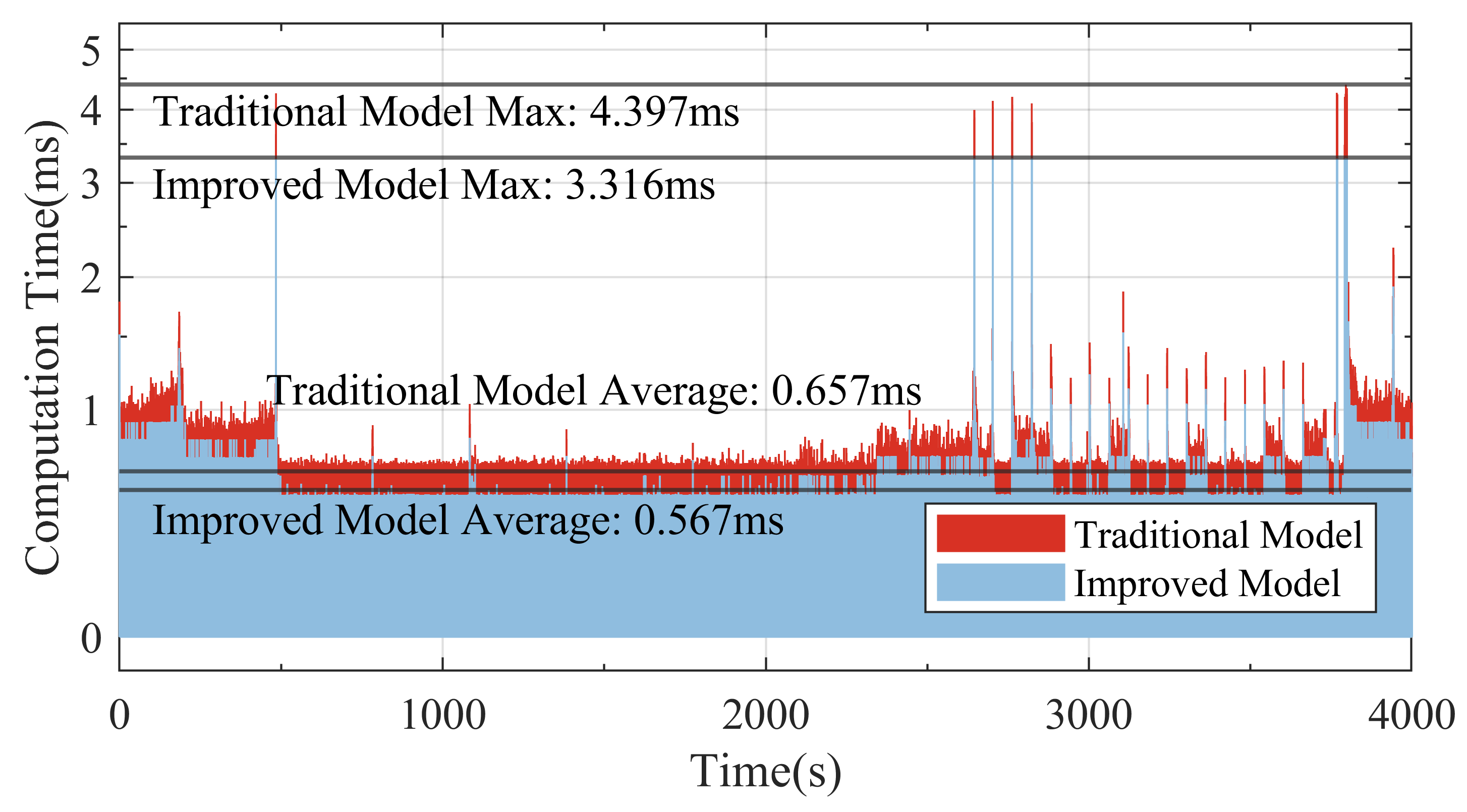
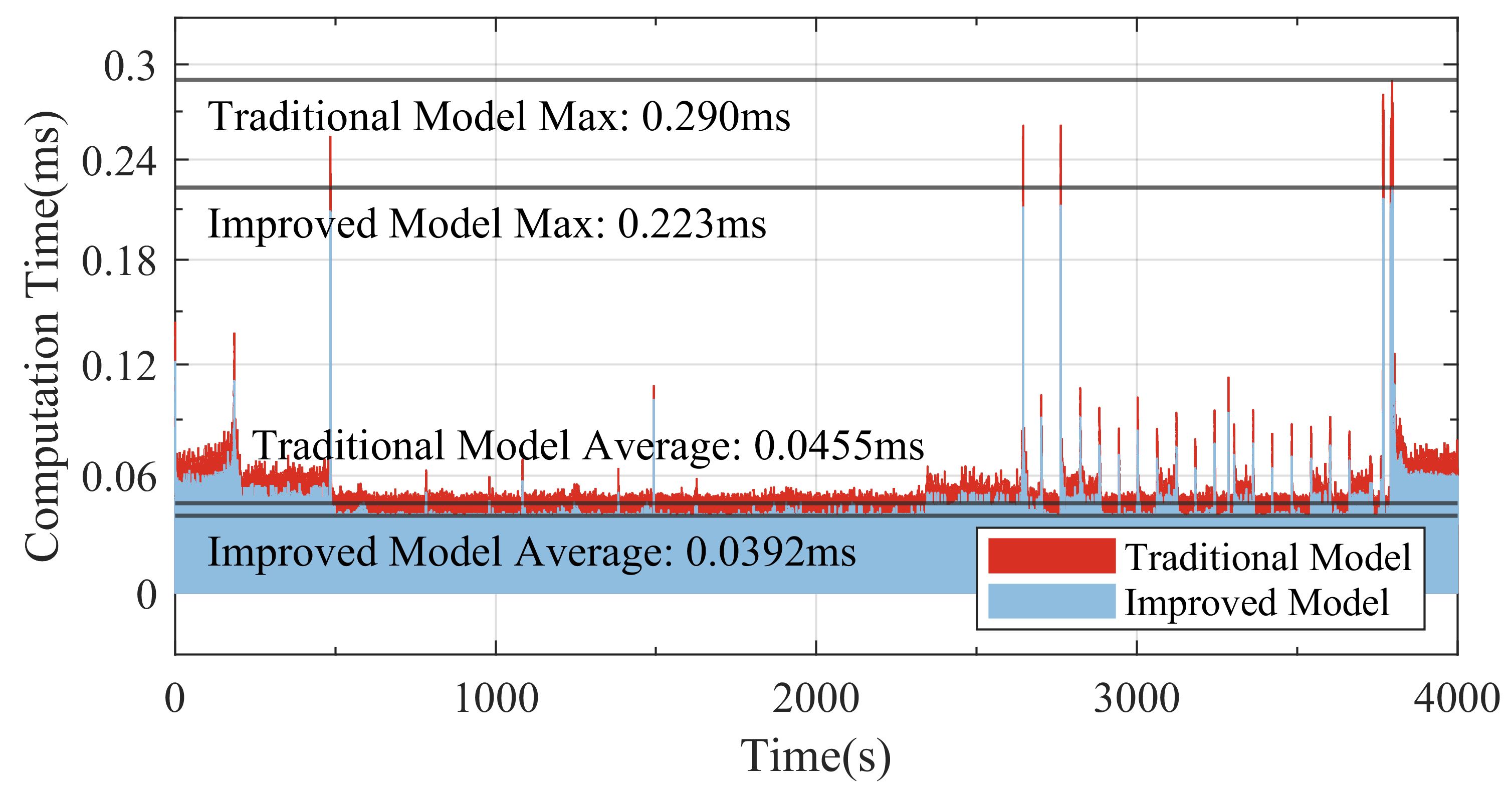
Figure 9 and Figure 10 show the computation time per simulation step for the idle-to-maximum condition test on the P2020 and Xeon8280 processors, respectively, comparing the traditional and nozzle-improved engine models. On the P2020 platform, the improved model reduces the maximum and average computation times to 3.316 ms and 0.567 ms per step, corresponding to reductions of $24.58\%$ and $13.7\%$ relative to the traditional model. On the Xeon8280 platform, the improved model achieves maximum and average computation times of 0.223 ms and 0.0392 ms per step, corresponding to reductions of $23.09\%$ and $13.8\%$ relative to the traditional model, respectively. The similar percentage improvements on both embedded and modern multicore architectures indicate that the nozzle optimization consistently reduces the computational cost of the engine model across different platforms.

5. Conclusions

This study analyzes the limitations of traditional zero-dimensional nozzle models and proposes a non-iterative zero-dimensional nozzle model. The proposed model was subsequently applied to a turbofan engine model and validated through numerical simulations. Based on the results, the following conclusions can be drawn:

1.

Traditional nozzle models, due to the limited accuracy of iterative solution methods, can produce discontinuous or non-monotonic mass-flow-rate versus available pressure-drop curves during the subcritical-to-choked transition flow regime. This behavior reduces the numerical convergence robustness of engine simulations operating in this regime.

2.

A non-iterative nozzle calculation method is proposed, which determines the flow regime (subcritical or choked) using the characteristic Mach number and flow factor, thereby eliminating iterative computation. Compared with the traditional nozzle model requiring 8 iterations via the bisection method, the proposed approach reduces computational time by 85.71% and produces a mass-flow-rate versus available pressure-drop curve that remains continuous and monotonic across the subcritical-to-choked transition flow regime.

3.

The non-iterative nozzle model was applied in dynamic simulations of a turbofan engine, covering the transition from idle to maximum power. The engine model using the non-iterative nozzle model achieves a 24.58% reduction in maximum per-step computation time and a 13.7% reduction in average per-step computation time relative to the traditional model, while maintaining comparable simulation accuracy.

Overall, the proposed non-iterative nozzle model significantly enhances the computational efficiency of component-level turbofan engine simulations, and it can be readily applied to other engine component models to improve real-time simulation performance.