Article

A Mamba-Based Hierarchical Partitioning Framework for Upper-Level Wind Field Reconstruction

by
Wantong Chen
,
Yifan Zhang
,
Ruihua Liu
,
Shuguang Sun
and
Qing Feng
*
School of Electronic Information and Automation, Civil Aviation University of China, Tianjin 300300, China
*
Author to whom correspondence should be addressed.
Aerospace 2025, 12(9), 842; https://doi.org/10.3390/aerospace12090842
Submission received: 7 August 2025 / Revised: 3 September 2025 / Accepted: 16 September 2025 / Published: 18 September 2025
(This article belongs to the Section Air Traffic and Transportation)

Abstract

An accurate perception of upper-level wind fields is essential for improving civil aviation safety and route optimization. However, the sparsity of observational data and the structural complexity of wind fields make reconstruction highly challenging. To address this, we propose QuadMamba-WindNet (QMW-Net), a structure-enhanced deep neural network that integrates a hierarchical state-space modeling framework with a learnable quad-tree-based regional partitioning mechanism, enabling multi-scale adaptive encoding and efficient dynamic modeling. The model is trained end-to-end on ERA5 reanalysis data and validated with simulated flight trajectory observation masks, allowing the reconstruction of complete horizontal wind fields at target altitude levels. Experimental results show that QMW-Net achieves a mean absolute error (MAE) of 1.62 m/s and a mean relative error (MRE) of 6.68% for wind speed reconstruction at 300 hPa, with a mean directional error of 4.85° and an R 2 of 0.93, demonstrating high accuracy and stable error convergence. Compared with Physics-Informed Neural Networks (PINNs) and Gaussian Process Regression (GPR), QMW-Net delivers superior predictive performance and generalization across multiple test sets. The proposed model provides refined wind field support for civil aviation forecasting and trajectory planning, and shows potential for broader applications in high-dynamic flight environments and atmospheric sensing.

1. Introduction

Upper-level wind fields are critical meteorological variables that significantly influence aircraft performance and flight safety, and their importance for aviation meteorology has been comprehensively reviewed in recent surveys [1]. They play a vital role in civil aviation route planning, air traffic management, and mission support for military operations. High-temporal-resolution and accurate wind information improves the real-time responsiveness of trajectory optimization and simultaneously enhances energy efficiency and operational effectiveness while ensuring flight safety [2]. However, current mainstream meteorological observation systems still face limitations in providing timely and high-resolution wind field data. Although geostationary satellites offer wide-area coverage and are indispensable in global monitoring, their remote sensing inversion accuracy remains constrained by algorithmic modeling capabilities and observation conditions [3]. Some studies have developed high-precision tropospheric slant delay models based on ERA5 reanalysis data, which demonstrate strong adaptability and error control across diverse terrain types, providing a reliable data foundation for wind field modeling and reconstruction tasks [4].
High-resolution wind observations are widely recognized as essential for advancing numerical weather prediction (NWP) and ensuring flight safety. Yet such capabilities remain constrained by payload technology and have not been fully realized on spaceborne platforms [5]. Radiosondes provide accurate vertical profiles, but their low launch frequency and sparse spatial coverage limit their value for aviation meteorological services that require continuous real-time data [6]. NWP, which relies on observational data and solutions to complex physical equations, is crucial for medium- to long-range forecasting. However, it is less effective at producing rapid wind field updates, making it poorly suited to dynamic conditions and real-time flight assurance [7]. Moreover, recent studies emphasize the variability of NWP outputs, and overreliance on model reliability can amplify errors under rapidly changing wind conditions, reducing its support for real-time wind field modeling [7,8].
With advances in airborne surveillance technology, researchers have begun leveraging data from Automatic Dependent Surveillance–Broadcast (ADS-B) and Mode S [9,10,11,12] to enhance the spatiotemporal resolution and timeliness of wind field estimation. These data provide high-frequency flight trajectory and aircraft state information, offering a novel means for reconstructing key meteorological elements such as wind speed and direction. They have been widely applied in wind estimation and aircraft performance analysis [9]. For example, the Meteo-Particle model, developed using such data, has demonstrated significantly improved performance in localized wind–temperature field reconstruction relative to traditional reanalysis-based interpolation methods [10]. Other studies have employed Gaussian Process Regression (GPR) for continuous wind vector estimation across arbitrary spatiotemporal positions using ADS-B and Mode S data, enabling real-time updates with uncertainty quantification. Furthermore, the integration of polynomial chaos expansion techniques has improved global structural modeling of wind fields, enabling the mesh-free modeling and rapid assimilation of new observational data, thus supporting short-term forecasting and trajectory optimization [11,12]. Despite the strong fitting and uncertainty representation capabilities of GPR, its computational efficiency is relatively low, and prediction reliability declines in areas with sparse or missing trajectory data.
In response to the challenges posed by sparse observations and complex atmospheric dynamics, recent studies have increasingly explored the application of deep learning methods to wind field modeling. Deep neural networks (DNNs) offer clear advantages in capturing nonlinear dependencies, extracting spatiotemporal features, and adapting to variable environmental conditions. For instance, Radial Basis Function (RBF) networks combined with Long Short-Term Memory (LSTM) architectures have been employed to construct adaptive wind speed prediction models capable of real-time and short-term forecasting [13]. Temporal Convolutional Networks (TCNs) have been applied to mid- to long-term wind modeling [14], while Convolutional Neural Networks (CNNs) enhanced by evolutionary algorithms have improved short-term prediction accuracy [15]. More recently, Transformer-based architectures have been used for wind speed forecasting [16], incorporating variational mode decomposition and optimization strategies to enhance both temporal feature learning and interpretability.
Despite their predictive strength, these purely data-driven methods often struggle to maintain physical consistency, especially when dealing with sparse or non-uniform observations. To address these limitations, researchers have introduced physics-guided approaches that integrate domain knowledge directly into the learning process. For example, satellite-derived cloud motion vectors have been used to support neural network-based wind field reconstruction [17], and Physics-Informed Neural Networks (PINNs) [18] embed physical constraints into the loss function to improve temporal continuity and physical plausibility. Compared with traditional numerical and particle-based methods, PINNs achieve lower wind speed and direction errors and support near-real-time estimation. Additionally, recent studies have introduced physics-aware attention mechanisms to improve the consistency and scalability of multi-resolution wind field modeling [19]. While these methods share the goal of enhancing structural representation under sparse observation conditions, they depend heavily on pre-defined physical constraints and external numerical weather prediction (NWP) inputs, which limit their independence and generalization. Furthermore, they often require the manual hyperparameter tuning of the physical loss terms, increasing deployment complexity and cost.
Building on earlier work with data-driven and physics-guided methods, recent studies have emphasized the advantages of optimization-driven and hybrid frameworks for improving predictive accuracy under sparse observational conditions. For example, ref. [20] developed a hybrid data assimilation–machine learning (DA–ML) framework within the WRF model that integrates multisource soil moisture and leaf area index observations, resulting in an improved simulation of complex land–atmosphere interactions. Similarly, ref. [21] combined the Informer deep learning network with WRF-Hydro in a hybrid scheme, achieving higher runoff prediction skill (NSE = 0.66–0.76) in data-sparse catchments. Hybrid hydroclimatic forecasting systems that couple dynamical model outputs with machine learning have also been shown to improve the prediction of rainfall and streamflow extremes [22]. In addition, ref. [23] proposed a hybrid data assimilation (HDA–ML) framework that incorporates CNNs into traditional workflows such as 4DVar and EnKF, enabling more accurate atmospheric state estimation at lower computational cost. Taken together, these studies demonstrate that optimization-oriented and hybrid strategies can strengthen model robustness and generalization, providing motivation for the structured, optimization-informed design of QMW-Net for wind field reconstruction under sparse observations.
In parallel with these optimization-driven advances, recent studies in the wind field domain have examined multi-source data fusion and three-dimensional reconstruction strategies. Recent work has investigated three-dimensional wind field reconstruction through multi-source data fusion and deep learning, demonstrating the benefits of integrating ground-based and satellite observations [24,25]. Such methods enhance vertical continuity and improve large-scale estimation accuracy, yet they often depend heavily on external observation networks and involve high computational costs, which limit their practicality in real-time aviation scenarios. Moreover, most existing studies have not explicitly addressed flight-level constraints, leaving uncertainty about how reconstructed fields align with operationally relevant cruise altitudes. Consequently, despite gains in accuracy, current methods continue to face challenges with sparse and irregular aviation observations, particularly at typical en-route flight levels where reliable wind information is most critical.
To address this gap, the present study focuses on wind field reconstruction at the 300 hPa pressure level, which corresponds approximately to flight level FL300 (30,000 ft, or 9 km MSL). This altitude is a typical en-route cruise level for commercial airliners and lies near the upper boundary of the troposphere, where complex regional wind patterns and jet stream structures frequently occur. Targeting this layer thus ensures both aviation relevance and sufficient variability for evaluating model robustness. Motivated by these considerations, we propose a novel deep neural network, QuadMamba-WindNet (QMW-Net), which combines structured state-space modeling with a learnable hierarchical region-partitioning mechanism for high-resolution horizontal wind field reconstruction. Built on the recently introduced QuadMamba framework [26], the model is specifically designed to address the spatial sparsity and structural complexity of upper-level wind measurements. Recent studies have shown the effectiveness of Mamba and its variants in high-dimensional tasks such as hyperspectral image classification, providing inspiration for our model design [27].
Compared to conventional convolutional or Transformer-based models, QMW-Net adopts a linear state-space computation scheme to improve inference efficiency. In contrast to fixed-window methods such as LocalMamba, it introduces a differentiable quad-tree partitioning strategy that adaptively adjusts modeling granularity according to the spatial distribution of observations [28]. This enables QMW-Net to balance fine-grained feature extraction with global structural modeling, making it particularly effective for sparse wind field scenarios. The overall architecture is designed to balance predictive accuracy, computational cost, and spatial adaptability, thereby supporting real-time upper-level wind field reconstruction and forecasting in flight operations. The rest of this paper is organized as follows. Section 2 presents the unified Materials and Methods, including the QMW-Net architecture, data collection, evaluation metrics, baseline models, and the experimental setup with reconstruction and robustness results. Section 3 concludes with the main findings, limitations, and potential applications in aviation meteorology and high-resolution wind field modeling.

2. Materials and Methods

2.1. Model Architecture

QuadMamba-WindNet (QMW-Net) is a structure-enhanced deep neural network developed to efficiently and accurately reconstruct upper-level horizontal wind fields from sparse observations. The architecture consists of four main components: an encoder, a region-partitioning and -fusion module, a state-modeling module, and a reconstruction module. The encoding stage begins with a lightweight mapper that extracts spatial features from the raw observed wind field tensor. A 2D score map is then generated using a region scoring function, which guides a learnable quad-tree partitioning mechanism. This mechanism recursively divides the tensor into coarse- and fine-grained sub-windows. Adaptive average pooling and Gumbel–Softmax are applied to construct region fusion masks, allowing for the weighted aggregation of multi-scale window features and producing a compact, continuous, one-dimensional feature sequence.
Since the Mamba-based state modeling module requires structurally coherent input, the fused sequence is upsampled to the original spatial resolution before entering the modeling stage. This upsampling improves spatial order consistency and supports more stable temporal dynamics. The Mamba module itself efficiently captures dynamic propagation patterns and long-range dependencies within the wind field, thereby strengthening the model’s structural understanding. To reduce boundary artifacts introduced by regional partitioning, a multi-directional window-shifting mechanism is incorporated to promote contextual continuity.
Finally, a linear transformation is applied to produce the predicted wind velocity tensor ( u , v ) in the original spatial domain. The proposed architecture achieves a balance between structural continuity and predictive accuracy while maintaining high computational efficiency, making it well-suited for modeling complex and variable upper-level wind environments.

2.1.1. Mathematical Model

This paper introduces a state-space model (SSM) as the core framework for modeling temporal dynamics in regional wind fields using one-dimensional feature sequences. The recently proposed Mamba module is adopted, which relies on a selective state-space formulation and employs convolution kernel reparameterization for efficient input–response modeling. This design is particularly well-suited to scenarios involving dynamic propagation and long-range wind field reconstruction.
Fundamentally, the state-space model (SSM) can be expressed as a linear time-invariant system, where a one-dimensional input sequence x ( t ) R L is mapped to an output sequence y ( t ) R L  [29,30]. which can be described by the following equations:
h ( t ) = A h ( t ) + B x ( t ) ,
y ( t ) = C h ( t ) ,
where h ( t ) represents the hidden state vector, A and B are the state-transition and input-projection matrices, and C denotes the output-projection matrix. Because continuous-time systems are not directly applicable to deep learning training, we adopt zero-order hold (ZOH) discretization with step size Δ  [31,32], under which the discrete state matrices are given by
A ¯ = exp ( Δ A ) ,
B ¯ = A 1 exp ( Δ A ) I B ,
where exp ( · ) represents the matrix exponential and I is the identity matrix of appropriate dimension. Using Equations (3) and (4), the discrete-time state update and output equations can be written as
h t = A ¯ h t 1 + B ¯ x t ,
y t = C h t ,
where t denotes the discrete time step. To further enhance computational efficiency and parallelization, the Mamba module reformulates the recurrence in Equations (5) and (6) as a global one-dimensional convolution, with the kernel defined as
K ¯ = C B ¯ , C A ¯ B ¯ , , C A ¯ M 1 B ¯ ,
so that the output can be written as
y = x K ¯ ,
where ∗ denotes one-dimensional convolution, M is the length of the input sequence, and K ¯ R M is the associated convolution kernel.

2.1.2. Wind State Construction and Prediction Based on QuadMamba

To enhance the ability of the Mamba-based state-space module to capture internal structures and multi-scale features in wind field subregions, we introduce a pre-structured spatial partitioning mechanism. This mechanism enables the module to adaptively control spatial granularity during sequence encoding. It operates directly on the original wind field tensor through a learnable quad-tree partitioning strategy, which provides region-aware decomposition and feature enhancement. Consequently, a unified spatial structure is obtained, ensuring consistency between the partitioning process and subsequent dynamic modeling. The original wind field tensor is denoted as
F R H × W × C , C = 2
where H and W denote the spatial resolutions in the latitudinal and longitudinal directions, respectively, and the two channels correspond to the u and v wind components. To initialize region scoring and spatial structure modeling, the input tensor is passed through a lightweight embedding function φ s as
F s = φ s ( F ) , F s R H × W × C ,
where φ s is implemented as a shallow feed-forward network consisting of normalization layers, linear projections, and nonlinear activation functions, which enable lightweight feature extraction while preserving essential spatial information. To further disentangle structural cues, the embedded tensor is split along the channel dimension into local and global parts, allowing the model to capture fine-grained regional details and broader contextual dependencies in parallel:
F s local = F s [ : , : , 0 : C 2 ] , F s global = F s [ : , : , C 2 : C ] , { F s local , F s global } R H × W × C 2 ,
where the colon operator [ : , : ] preserves the spatial dimensions and splits the channel dimension for subsequent local scoring and global modeling. To capture coarse-grained spatial cues, a 2 × 2 adaptive average pooling is applied to the local feature tensor, yielding
v s local = AdaptiveAvgPool 2 D ( F s local ) , v s local R 2 × 2 × C / 2 ,
where v s local represents a coarse structural abstraction of local regions. Each element corresponds to the average response of a spatial subregion, which can be formally expressed for channel c at region ( i , j ) as
v s local i , j , c = 1 | R i , j | ( h , w ) R i , j F s local h , w , c ,
where R i , j denotes the set of pixel indices within the ( i , j ) pooling region of the original feature map. This ensures that each element of v s local corresponds to the average response of its respective subregion while preserving channel-wise representation capacity. Since these pooled descriptors have only 2 × 2 resolution, they must be restored to the original spatial size to align with the global features. To accomplish this, v s local is bilinearly upsampled, defined as
v ˜ s local ( h , w , c ) = i = 1 2 j = 1 2 W i j ( h , w ) · v s local ( i , j , c ) , v ˜ s local R H × W × C / 2 .
where W i j ( h , w ) are the bilinear interpolation weights for the ( h , w ) position relative to the pooling coordinates ( i , j ) , satisfying i , j W i j ( h , w ) = 1 to guarantee spatial smoothness and interpolation consistency. Finally, the interpolated local features are concatenated with the global features along the channel dimension to form the fused tensor:
F s agg ( h , w , : ) = F s global ( h , w , : ) , v ˜ s local ( h , w , : ) , F s agg R H × W × C .
To guide the subsequent quad-tree partitioning, we first generate a probability distribution over coarse and fine regions for each spatial location. Specifically, the fused tensor is projected through a linear layer φ p and then passed to a Softmax activation:
s = Softmax ( φ p ( F s agg ) ) , s R H × W × 2 .
These probability maps serve as location-wise indicators of whether a region should be modeled at a coarse or fine resolution. Guided by these scores, the quad-tree partitioning procedure adaptively controls spatial granularity while maintaining low computational cost. In practice, the process proceeds hierarchically: the input tensor is first divided into coarse sub-windows, their importance is evaluated through pooled scores, the most informative region is selected, and this region is then recursively subdivided into finer windows.
{ w N 1 i i = 0 , 1 , 2 , 3 } = QuadWindowPartition ( F ) , w N 1 i R H 2 × W 2 × C , { s N 1 i i = 0 , 1 , 2 , 3 } = AdaptiveAvgPool 2 D QuadWindowPartition ( s ) , k = TopK ( { s N 1 i } , K = 1 ) , i { 0 , 1 , 2 , 3 } , { w N 2 ( k , j ) j = 0 , 1 , 2 , 3 } = QuadWindowPartition ( w N 1 k ) .
Here, w N 1 i denote coarse windows of size ( H / 2 , W / 2 ) and w N 2 ( k , j ) denote fine windows of size ( H / 4 , W / 4 ) . This hierarchical decomposition provides a coarse-to-fine representation that serves as input to the subsequent Mamba-based state modeling. To enable the end-to-end training of the partitioning process, the hard decision of selecting a single region is replaced with a differentiable alternative. For this purpose, we adopt the Gumbel–Softmax mechanism [33], which provides a soft approximation to one-hot selection while still allowing gradient backpropagation. Given the set of sub-window scores { s N 1 i } , the mask for the first-level partition is computed as
M 1 = GumbelSoftmax { s N 1 i i = 0 , 1 , 2 , 3 } , M 1 { 0 , 1 } 2 × 2 × 1 .
Here, M 1 acts as a binary mask indicating which regions are further subdivided (1) and which remain at the coarse level (0). In practice, M 1 is generated by sampling from the score distribution of the four candidate regions using the Gumbel–Softmax trick. For each candidate region i, the soft assignment is defined as
y i = exp ( z i + g i ) / τ j = 1 4 exp ( z j + g j ) / τ , g i = log ( log ( U i ) ) , U i Uniform ( 0 , 1 ) ,
where z i is the logit score of region i, g i is Gumbel noise, and τ > 0 is the temperature parameter controlling smoothness. Collecting the four outputs { y 1 , y 2 , y 3 , y 4 } yields the mask M 1 , which provides a differentiable approximation to one-hot selection and thereby supports gradient propagation during training. Guided by the mask M 1 , the original wind field tensor F is arranged into hierarchical window sequences. Specifically, coarse windows ( L 1 ) span the entire field at resolution ( H / 2 , W / 2 ) , while fine windows ( L 2 ) further refine the selected subregions:
L 1 = QuadWindowArrange ( F ( H / 2 , W / 2 ) ) ,
L 2 = QuadWindowArrange ( Restore ( L 1 ) ( H / 4 , W / 4 ) ) .
Here, the operator QuadWindowArrange ( · ( h , w ) ) partitions F R H × W × C into non-overlapping windows of size ( h , w ) and flattens each window:
QuadWindowArrange ( F ( h , w ) ) = Flatten ( QuadWindowPartition ( F , h , w ) ) ,
Formally, each sub-window F i j R h × w × C is flattened into a one-dimensional vector x i j R h w · C by mapping its 2D spatial indices ( p , q ) and channel index d into a single sequence index k:
x i j [ k ] = F i j ( p , q , d ) , k = ( p · w + q ) · C + d .
This mapping ensures that the spatial and channel information from each sub-window is preserved in raster-scan order when converted into sequential form, so that the resulting sequence L remains structurally consistent with the original wind field tensor. All x i j vectors are concatenated to form the sequence L , while the inverse operator Restore ( · ) reconstructs the spatial tensor for further subdivision. The coarse mask M R H × W × 1 is upsampled to match the resolution of the feature sequences and applied through element-wise multiplication, producing a fusion of coarse- and fine-level features:
L = ( M L 2 ) ( 1 M ) L 1 ,
where ⊙ denotes element-wise multiplication and ⊕ denotes sequence concatenation. When windows are partitioned strictly along grid boundaries, discontinuities may occur at the edges, causing adjacent regions to be modeled in isolation. To mitigate this issue and enhance continuity across boundaries, a shifted-window scheme is introduced. In this scheme, alternate layers apply horizontal or vertical shifts to the partitioning grid, so that boundary pixels in one layer become interior pixels in the next, thereby enabling effective context exchange across neighboring regions. Formally, for a window of size ( h , w ) , the shifted feature tensor is defined as
F shifted = Roll ( F , ( δ h , δ w ) ) , δ h = h / 2 , δ w = w / 2 ,
where Roll ( · ) cyclically shifts the feature map by ( δ h , δ w ) along the spatial axes. This operation enables the model to capture cross-window dependencies and mitigates artifacts at coarse–fine region boundaries. The fused sequence L is subsequently passed to the Mamba module for dynamic state-space modeling, yielding
L out = Mamba ( L ) .
Finally, the output sequence is reshaped back into the spatial tensor domain:
F ^ = Reshape ( L ) , F ^ R H × W × 2 .
Here, the reshape operator converts the sequential features back into a spatial tensor of dimensions ( H , W , 2 ) , corresponding to the predicted wind components. This step ensures consistency between spatial and sequential structures, providing a unified decoding process for multi-resolution regions and thereby improving the continuity and predictive accuracy of wind field reconstruction. The overall computation flow of QMW-Net is summarized in Algorithm 1, where the model builds on the structure-enhanced QuadMamba framework, integrating a learnable spatial partitioning mechanism with dynamic modeling capabilities to improve both accuracy and efficiency in wind field reconstruction.
The model first introduces a hierarchical quad-tree partitioning mechanism guided by region scores, enabling the adaptive extraction of key spatial features at multiple granularity levels. Then, a Gumbel–Softmax mask is employed to perform importance selection and the fusion of coarse- and fine-grained feature sequences. The fused result is interpolated back to the original spatial resolution, forming a continuous and compact input sequence. This sequence is then passed to the Mamba state-space modeling module to capture contextual spatial structures, after which a reshape operation restores the wind field tensor, yielding high-resolution wind field reconstruction.
Algorithm 1 QuadMamba-WindNet Wind Field Reconstruction Pipeline.
Require: 
Observed wind field tensor F R H × W × 2
Ensure: 
Predicted wind field tensor F ^ R H × W × 2
1:
/* Step 1: Embedding and Feature Extraction */
2:
F embed PatchEmbed ( F )
3:
F s φ s ( F embed )
4:
/* Step 2: Region Scoring and Aggregation */
5:
[ F s local , F s global ] SplitChannels ( F s )
6:
v s local AdaptiveAvgPool 2 D ( F s local )
7:
F s agg Concat ( F s global , Interpolate ( v s local ) )
8:
s Softmax ( φ p ( F s agg ) )
9:
/* Step 3: Quadtree Partition and Selection */
10:
{ w N 1 i i = 0 , 1 , 2 , 3 } QuadWindowPartition ( F )
11:
for  i = 0 , 1 , 2 , 3 do
12:
     s N 1 i AdaptiveAvgPool 2 D ( QuadWindowPartition ( s ) )
13:
end for
14:
k TopK ( s N 1 i , K = 1 )
15:
W N 2 ( k , j ) QuadWindowPartition ( W N 1 k )
16:
/* Step 4: Gumbel–Softmax Masking and Sequence Construction */
17:
M 1 GumbelSoftmax ( { s N 1 i i = 0 , 1 , 2 , 3 } )
18:
L 1 QuadWindowArrange ( F H 2 , W 2 )
19:
L 2 QuadWindowArrange ( Restore ( L 1 ) H 4 , W 4 )
20:
L ( M 1 L 2 ) ( ( 1 M 1 ) L 1 )
21:
/* Step 5: State Modeling and Output */
22:
L out Mamba ( L )
23:
F ^ Reshape ( L out )
24:
return  F ^

2.2. Data Collection

ERA5, developed by the European Centre for Medium-Range Weather Forecasts (ECMWF), is the fifth-generation global reanalysis dataset that integrates physical laws with worldwide observational data through numerical weather prediction (NWP) models. It provides high-resolution global meteorological data with both hourly updates and a spatial resolution of 0 . 25 ° × 0 . 25 ° on a latitude–longitude grid. The dataset spans 37 pressure levels, ranging from 1 hPa to 1000 hPa. In this study, we use ERA5 data as the foundational dataset and further process it to meet the requirements of wind field reconstruction tasks.
Because the model must learn the global wind field distribution from limited observed samples, we propose a mask construction method based on sparse sampling to simulate the process of local wind field observations. Specifically, we define an all-zero matrix O R H × W as the background field. Then, through a random process S = { s t } t = 1 n , we generate n sampling trajectories. For each trajectory S k ( k = 1 , 2 , , n ) , the corresponding positions in O are set to 1, while all other positions remain zero. Based on this, we construct a binary mask matrix M { 0 , 1 } H × W and subsequently apply an element-wise Hadamard product to compute
W mask = M W
This operation extracts sparse observations along the simulated trajectories from the complete wind field data W, treating W mask as the model input and using the full wind field W as the supervised target to guide model learning and optimization.

2.3. Evaluation Metrics

To comprehensively evaluate the performance of the wind field reconstruction model, multiple evaluation metrics are employed to quantify prediction errors and fitting ability for both wind speed and wind direction. The first metric is the Mean Absolute Error (MAE), which measures the average magnitude of absolute errors between the predicted and true values:
MAE = 1 N i = 1 N | y ^ i y i | ,
where y i and y ^ i denote the true and predicted wind speed of the i-th sample, respectively, and N is the total number of samples. MAE reflects the average prediction bias in wind speed estimation, with lower values indicating closer agreement with the ground truth. In addition, the Root Mean Square Error (RMSE) applies a squared penalty to the errors, making it more sensitive to large deviations:
RMSE = 1 N i = 1 N ( y i y ^ i ) 2 ,
where a higher RMSE indicates poor performance, particularly in regions with abrupt wind speed changes. For wind direction prediction, due to the periodic nature of directional data, we adopt a directional MAE that computes the smallest angular difference between predicted and actual wind directions, ensuring that the error lies within [ 0 ° , 180 ° ] :
MAE direction = 1 N i = 1 N min | θ i θ ^ i | , 360 ° | θ i θ ^ i | ,
where θ ^ i and θ i represent the predicted and true wind directions of the i-th sample, respectively. This metric effectively handles the periodicity of angular data by computing the minimum angular difference. To evaluate performance across different wind speed scales, we also adopt the Mean Relative Error (MRE):
MRE = i = 1 N | y i y ^ i | i = 1 N | y i | ,
which provides a normalized error metric and allows consistent comparison across different datasets and magnitudes. Finally, the coefficient of determination ( R 2 ) is used to assess how well the predicted values fit the true wind speed data:
R 2 = 1 i = 1 N ( y i y ^ i ) 2 i = 1 N ( y i y ¯ ) 2 ,
where y ¯ denotes the mean of the ground-truth values. A higher R 2 indicates better model performance and stronger explanatory power.

2.4. Baseline Models

2.4.1. Physics-Informed Neural Network (PINN)

The Physics-Informed Neural Network (PINN) is a class of model that incorporates physical constraints into deep learning frameworks. It adopts a U-Net architecture in which standard convolution operations are replaced with partial convolutions to better handle irregular and sparse data distributions. By embedding multiple physical laws into the loss function, PINNs preserve physical consistency throughout the data-driven prediction process, thereby improving robustness and interpretability. They are particularly well-suited to scenarios with limited or low-quality observational data, achieving high predictive accuracy and strong generalization in wind field reconstruction tasks [28].

2.4.2. Gaussian Process Regression (GPR)

Gaussian Process Regression (GPR) is a probabilistic machine learning method that assumes that the true distribution of the wind field follows a prior Gaussian process. By analyzing existing wind field observations, the GPR model iteratively optimizes the mean and covariance functions to compute the posterior distribution, thereby inferring the complete horizontal wind field. One of the primary advantages of GPR lies in its ability to quantify uncertainty, as it provides reliable confidence intervals for each predicted value. Nevertheless, GPR has limitations, particularly when applied to complex or non-Gaussian wind field characteristics. Because of its reliance on the Gaussian assumption, the model may fail to fully capture the underlying structure of such complex features [34].

2.5. Experimental Setup

The experimental setup of QMW-Net is designed to validate the proposed method, including parameter settings, wind field reconstruction results, and performance evaluation using metrics such as MAE. Experiments are conducted on the ERA5 dataset. Following the method in Section 2.2, input features and labels are derived from wind speed components u and v at the 300 hPa pressure level. The training data span the years 2019 to 2021 and cover the region from 3 ° E to 8 ° E longitude and 49 ° N to 54 ° N latitude, with a spatial resolution of 0 . 25 ° (approximately 10–15 nautical miles, nM, at 50° N, a commonly used navigational unit in aviation). Because the physical distance of one degree of longitude decreases with latitude, the spacing is not uniform between the east–west and north–south directions: 0.25° of latitude corresponds to about 15 nM, whereas the same spacing in longitude corresponds to about 11 nM in the European test region. Data from 2022 are reserved for testing, and a fixed random seed is applied to ensure reproducibility.
Model training uses the AdamW optimizer with a learning rate of 4 × 10 4 , momentum of 0.85, and weight decay of 0.03, with a batch size of 256. Training is conducted for 1000 epochs on an NVIDIA Quadro RTX 5000 GPU. As shown in Figure 1, the training loss decreases from 0.45 to 0.18 and the test loss decreases from 0.52 to 0.23 during the first 100 epochs, indicating that the model rapidly captures data features and establishes basic representational capacity. Between epochs 100 and 500, the training loss continues to decline to 0.12, while the test loss stabilizes around 0.15 ± 0.02 , suggesting that the model gradually enters a stable optimization phase. After 500 epochs, the training loss approaches 0.10 and the test loss remains stable, confirming convergence. The MAE metric is used to evaluate prediction accuracy. The test loss is consistently about 0.05 higher than the training loss, but the overall curve remains smooth. The final training loss stabilizes around 0.10, while the test loss remains near 0.15, demonstrating that the model achieves stable convergence performance within a controllable range.

2.6. Reconstruction Results

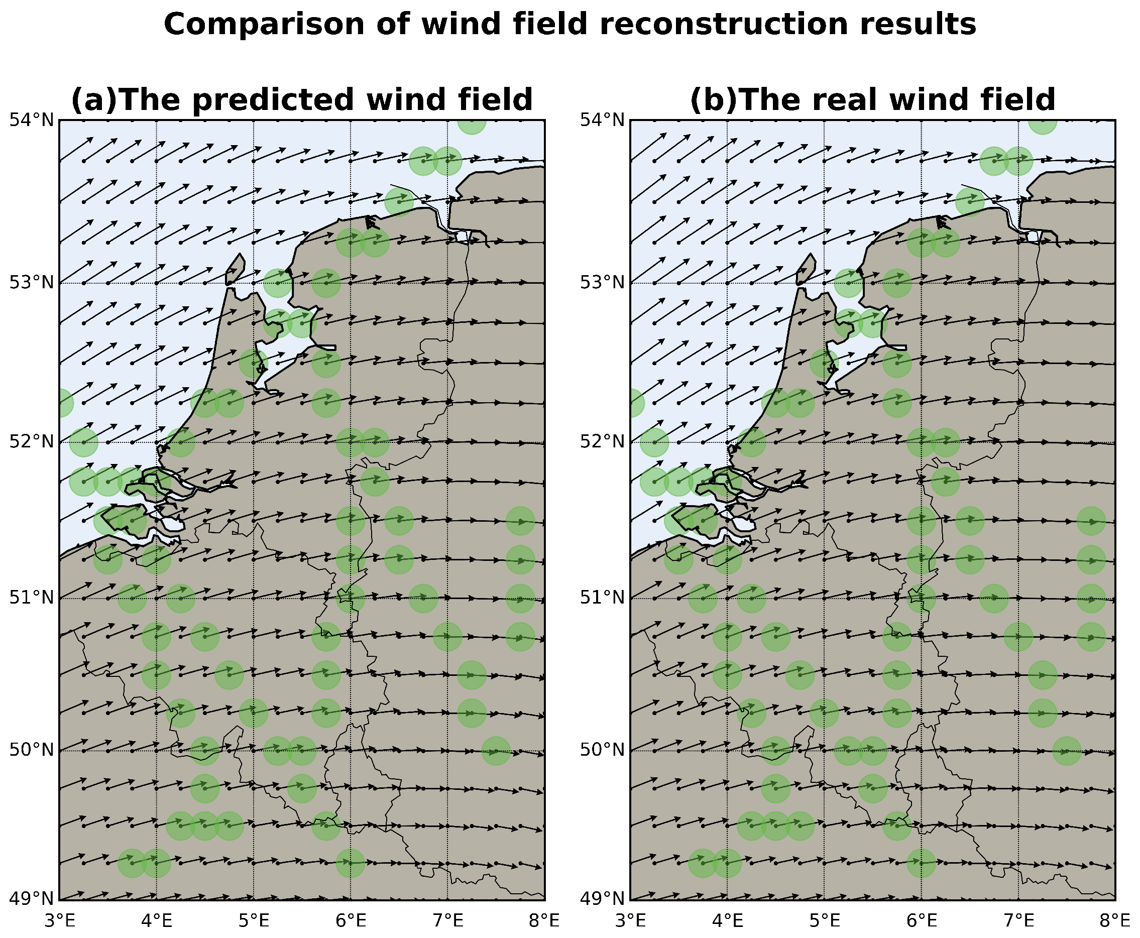
This section demonstrates the performance of the QMW-Net model on data not included in the training set, using a fixed random seed to ensure consistency in test results. Figure 2 presents the wind field reconstruction, where subfigures (A) and (B) show the u and v wind components, respectively. Panels (a), (b), and (c) represent the masked input (based on random trajectories), the predicted wind field, and the ground truth, while panel (d) shows the Mean Absolute Error (MAE) between the predicted and true values, with the average MAE calculated over all data points in meters per second (m/s). Beyond the average magnitude, the spatial distribution of residuals in panel (d) serves as a diagnostic of reconstruction accuracy. Although some clustered patterns appear, they primarily coincide with regions of strong wind shear and reflect the inherent variability of the ERA5 reference field rather than artifacts introduced by the model. The data correspond to the 300 hPa wind field at 12:00 on 1 February 2022, demonstrating that the model accurately reconstructs both u and v components, even in masked regions.
For a more intuitive visualization, the u and v components are converted into wind speed and direction and displayed as wind vectors on a geographical map, as shown in Figure 3. This reconstruction covers the region between 3° E–8° E and 49° N–54° N, corresponding to the Netherlands, Belgium, and western Germany, consistent with the spatial range of the original data. In Figure 3, dark brown areas represent land, light blue areas denote the sea, and green areas mark observed regions (those not masked). Each arrow represents a wind vector, with its direction and length corresponding to wind direction and speed. Compared with Figure 2, Figure 3 offers a clearer depiction of the spatial distribution of the reconstructed wind field. Subfigure (a) shows the wind field reconstructed by QMW-Net, while subfigure (b) presents the ERA5 reference field. Green dots indicate the observation locations, and black arrows represent wind vectors. Overall, the reconstructed wind field exhibits strong agreement with the reference in both wind direction distribution and wind speed gradient, demonstrating the model’s ability to effectively infer missing information in data-sparse regions and its robust spatial reconstruction capability.
To evaluate the effectiveness of the proposed model in reconstructing horizontal wind fields at typical cruise-level altitudes in civil aviation, we conducted experiments using the 300 hPa pressure level dataset from 2021. The evaluation focused on two key metrics: wind speed and wind direction. Results show that QMW-Net achieves high accuracy in both, further confirming its robustness and generalization under sparse upper-level observational conditions. Comprehensive performance metrics, including MAE, MRE, RMSE, and R 2 , are reported in Table 1.
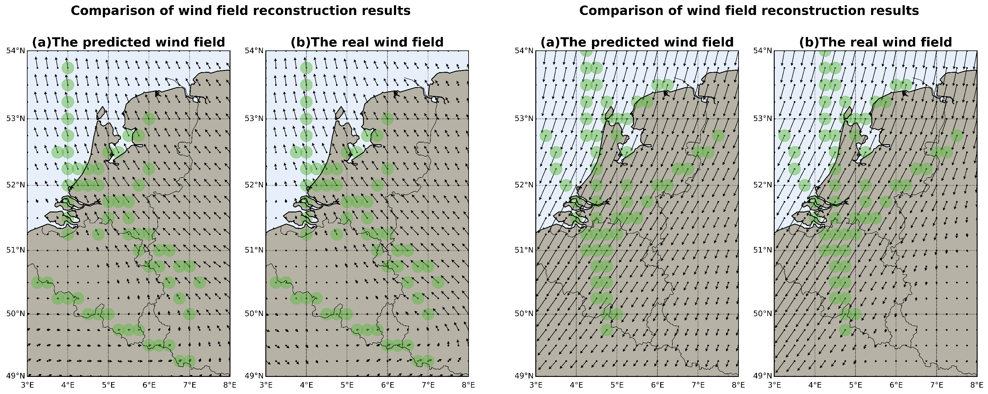
Despite the overall effectiveness of the model, complex flow field structures still pose challenges for wind field reconstruction. Figure 4 illustrates two representative wind field cases from the test set, generated using ERA5 reanalysis data as input for QMW-Net experiments. The left subfigure shows a relatively uniform wind speed distribution with localized changes in wind direction, whereas the right subfigure presents a more complex scenario involving the interaction of multiple airflows and pronounced wind speed gradients.
The comparison shows that the model is generally capable of reproducing the macroscopic distribution patterns of the wind field, successfully capturing the main wind direction trends and flow dynamics. Nevertheless, discrepancies between the predicted and actual wind fields remain in regions with sparse observations or strong wind variability. In particular, the model’s accuracy in estimating local wind speed and direction decreases under such conditions. This limitation is most evident in areas with sharp wind speed gradients or at the boundaries between different flow regimes, where the model shows a noticeable degree of deviation.
These findings indicate that, while the model demonstrates strong overall predictive performance, there is still room for improving the reconstruction of local wind features. Future work may focus on enhancing the integration of multi-source observational data and refining the representation of localized structures to further advance model performance.

2.7. Validation and Robustness Evaluation

For rigorous evaluation, QMW-Net is trained on ERA5 data from 2019–2021 and validated/tested on an independent 2022 split with no temporal overlap. In addition, 2018 data are used exclusively for generalization experiments against the baseline Gaussian Process Regression (GPR) model. All experiments follow a unified data partitioning strategy to prevent temporal leakage. Performance is assessed using MAE, RMSE, directional MAE, MRE, and R 2 , with each configuration repeated three times under fixed random seeds; we report the mean and standard deviation to account for randomness. Beyond this validation protocol, robustness experiments are further conducted to examine the model’s sensitivity under diverse test conditions.
To evaluate the robustness of the model under varying test conditions—specifically, its sensitivity to different environmental factors—this study constructs four representative test sets using observational data from both 2022 and 2018, ensuring comprehensive and reliable experimental results. The test datasets are built according to specific sampling strategies designed to capture variations in time, space, and pressure levels. The first test set consists of data from February, May, August, and November 2022, segmented by pressure levels into 37 sub-datasets spanning 100–800 hPa, and is used to evaluate the model’s adaptability across altitudes. The second test set uses the full-year 2022 data at the 300 hPa pressure level, focusing on model performance at typical cruising altitudes.
The third test set consists of data sampled at 12:00 UTC on September 1 and 15, as well as throughout October to December 2022 at 300 hPa, and is designed for comparative evaluation against the Physics-Informed Neural Network (PINN) model under consistent temporal conditions. The fourth test set extends to historical data from January to October 2018, sampled at 12:00 UTC on the first day of each month at 300 hPa, and is used to assess generalization capability through comparison with the Gaussian Process Regression (GPR) model. Together, these four test configurations provide a systematic framework for analyzing model stability under temporal and spatial variability, data sparsity, and diverse meteorological conditions, thereby offering strong support for evaluating the model’s reliability in practical aviation meteorology applications.

2.7.1. Sensitivity to Pressure Levels

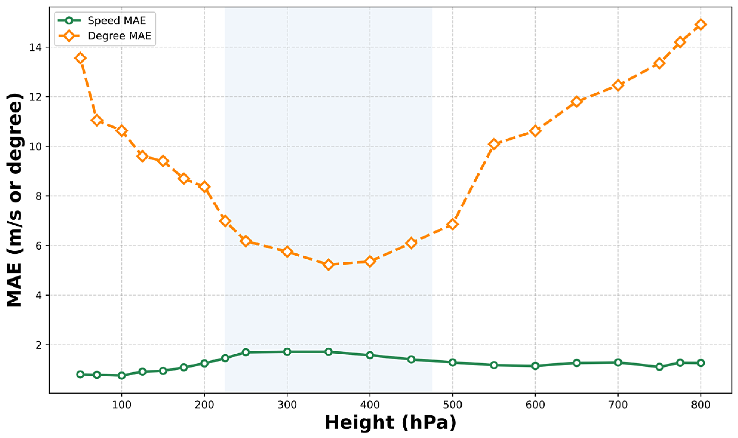
The pressure sensitivity of the model was evaluated using the first test set, which includes data sampled at three-month intervals to mitigate seasonal effects. Figure 5 illustrates the relationship between pressure levels and MAE (Mean Absolute Error), covering a pressure range from 50 hPa to 800 hPa (corresponding to altitudes of approximately 20,000 m to 2000 m, or about 65,000 ft to 6500 ft). The blue-shaded region highlights the typical cruising altitude range for civil aviation aircraft (225 hPa to 475 hPa), which is the primary focus of this study.
Figure 5 presents the Mean Absolute Error (MAE) of wind speed and direction at different pressure levels. The results show that the direction error (Degree MAE) is relatively high in lower-altitude regions (high-pressure zones) and gradually decreases with altitude. Within the blue-shaded range (225–475 hPa, corresponding to approximately 5400–11,300 m or 18,000–37,000 ft), the error becomes more stable, indicating better reconstruction performance for wind direction in this region. In contrast, the wind speed error (Speed MAE) remains relatively consistent across the entire vertical profile, suggesting strong robustness of the model in reconstructing wind speed.
At the typical cruising altitudes for civil aviation (approximately 225 to 475 hPa), both speed and direction errors remain low, indicating that the model performs well in reconstructing wind fields at these levels. This performance can be attributed to relatively stable meteorological conditions and smoother wind field variations within this altitude range. Overall, the results confirm that QMW-Net can effectively reconstruct wind field information at cruising levels, providing reliable data support for flight path optimization and aviation safety.

2.7.2. Sensitivity to Spatial Distance

This study quantitatively examines the factors influencing the accuracy of wind field prediction models. Results show that prediction and reconstruction errors, measured using the Mean Absolute Error (MAE), are strongly correlated with the spatial distance between the target grid point and the nearest observation station. To validate this relationship, a series of multidimensional error-tracing experiments were conducted on the second test set.
In each prediction instance, we recorded the spatial distance (denoted as variable X) between the predicted grid point and its closest observation, along with the corresponding MAE. Subsequently, the collected samples were grouped into distance-based layers using a 50 km interval. The experimental results are presented in Figure 6, which visually illustrates the trend of increasing prediction error as spatial distance increases. Moreover, the figure provides insights into the interdependence between wind vector direction and spatial distance, revealing the spatial dependence characteristics of wind field reconstruction performance.
As the prediction distance increases, both wind speed error (Speed MAE) and wind direction error (Degree MAE) show a clear upward trend, indicating higher uncertainty in long-distance predictions. Within shorter distances (0–150 km), the median values of speed and direction errors remain low, and the data distribution is relatively compact, reflecting stable model performance in this range. However, as the distance exceeds 200 km, the errors gradually increase and the spread of data becomes wider, suggesting a notable rise in prediction uncertainty. When the prediction distance reaches 500 km, the error level further increases, yet the distribution becomes more concentrated, implying improved stability despite the larger error magnitude. This trend indicates that the model’s predictive capacity diminishes with increasing spatial distance, highlighting the growing challenge of wind field reconstruction at longer ranges. Such degradation may result from data sparsity, limited model generalization, and the intrinsic complexity of spatiotemporal wind field variations.

2.7.3. Model Prediction Performance

Finally, to complement the validation and sensitivity analyses above, we perform a comparative evaluation against two representative baselines under unified experimental settings. Specifically, we consider the Gaussian Process Regression (GPR) model, trained on 2018 observational data, and the Physics-Informed Neural Network (PINN) model, trained on 2022 observational data [18,34]. All models are evaluated using the same data partitioning strategy to ensure fair and consistent comparison. In particular, the PINN model is tested on the third test set, comprising data collected at 12:00 on September 1 and 15 and daily from October through December 2022, while the GPR model is assessed on the fourth test set, which includes standardized observations sampled at 12:00 on the first day of each month from January to October 2018. For completeness, QMW-Net is evaluated on both datasets to provide a direct and balanced comparison.
The performance metrics for all models are summarized in Table 2 and Table 3. The experimental results clearly indicate that QMW-Net consistently surpasses the baseline models in predicting both wind speed and wind direction. Compared with the PINN model, QMW-Net achieves a 23.34% reduction in wind speed MAE and a 40.96% reduction in wind direction MAE. When compared with the GPR model, the reductions are even more pronounced—36.40% and 50.26%, respectively. These results highlight QMW-Net’s superior accuracy, strong generalization ability, and robust performance under diverse test conditions.

2.8. Discussion

The validation and robustness experiments demonstrate that QMW-Net achieves consistently lower errors than conventional baselines such as Gaussian Process Regression (GPR) and Physics-Informed Neural Networks (PINNs). Specifically, QMW-Net delivers significant improvements in both wind speed and wind direction reconstruction across multiple test sets, highlighting its ability to generalize under different temporal and spatial conditions. Compared with the GPR model, which incurs high computational cost and exhibits degraded performance in sparsely observed regions, QMW-Net maintains more stable accuracy by leveraging learnable hierarchical partitioning and structured state-space modeling. Relative to the PINN approach, QMW-Net reduces directional errors substantially, demonstrating its capability to capture spatiotemporal dependencies more effectively without relying on predefined physical constraints. These findings indicate that QMW-Net achieves a favorable trade-off between physical consistency and computational efficiency.
Beyond baseline comparisons, QMW-Net also demonstrates advantages over traditional deep learning methods reported in the literature, such as CNN-, RNN-, and Transformer-based architectures. While CNNs and TCNs perform well in local or short-term prediction tasks, they lack flexibility in handling sparse and irregular observations. Transformer-based methods enhance temporal feature learning but are computationally expensive for high-resolution meteorological data. In contrast, QMW-Net combines efficient linear state-space computation with adaptive quad-tree partitioning, enabling both scalability and structural awareness. Overall, these results show that QMW-Net not only outperforms representative baselines but also complements existing families of data-driven and physics-guided approaches, providing a robust framework for high-resolution wind field reconstruction under sparse observation scenarios and supporting applications in aviation meteorology and flight safety.

3. Conclusions

This study focuses on the reconstruction of upper-level wind fields at typical cruising altitudes in civil aviation and presents a comprehensive evaluation of the proposed QuadMamba-WindNet (QMW-Net) under sparse observation scenarios. Using the ERA5 reanalysis dataset, QMW-Net integrates limited trajectory-based measurements with a multi-scale encoding strategy and a lightweight reconstruction module to achieve continuous and accurate wind field recovery. Experiments conducted on the 2021 dataset at the 300 hPa pressure level demonstrate high accuracy, with a Mean Absolute Error of 1.62 m/s for wind speed and 4.85° for wind direction. Compared with baseline methods, error reductions reach 23.34% and 40.96% relative to the PINN model, and 36.40% and 50.26% relative to the GPR model, underscoring QMW-Net’s performance advantages.
Beyond overall accuracy, error analysis shows that performance declines when input observations are widely spaced or when wind fields contain sharp gradients, reflecting the intrinsic difficulty of reconstructing unobserved regions. Future work will therefore aim to improve generalization by incorporating a broader range of training conditions, such as extreme weather events and vertical (3D) wind field measurements. In addition, integrating physical constraints and real-time flight trajectory data into the learning process is expected to further enhance robustness, supporting high-resolution applications in short-term aviation weather forecasting and route optimization.

Author Contributions

Conceptualization, W.C. and Q.F.; methodology, W.C.; software, W.C.; validation, W.C., Y.Z. and R.L.; formal analysis, W.C.; investigation, Y.Z. and R.L.; resources, Q.F.; data curation, Y.Z. and S.S.; writing—original draft preparation, W.C. and Y.Z.; writing—review and editing, Q.F. and S.S.; visualization, Y.Z.; supervision, Q.F.; project administration, Q.F.; funding acquisition, Q.F. All authors have read and agreed to the published version of the manuscript.

Funding

This work was supported in part by the National Natural Science Foundation of China Civil Aviation Joint Fund Key Project under Grant U2233215, in part by the Fundamental Research Funds for the Central Universities under Grant 3122025088, and in part by the Civil Aviation Universiry of China Graduate Research Innovation Project under Grant 2024YJSKC02010.

Institutional Review Board Statement

Not applicable.

Informed Consent Statement

Not applicable.

Data Availability Statement

The original data presented in the study were made publicly available by the European Centre for Medium-Range Weather Forecasts (ECMWF) under the ERA5 dataset at https://doi.org/10.24381/cds.bd0915c6 (accessed on 6 July 2025).

Conflicts of Interest

The authors declare no conflicts of interest.

References

  1. Song, W.; Ye, X. A Comprehensive Review of Advances in Civil Aviation Meteorological Services. Atmosphere 2025, 16, 1014. [Google Scholar] [CrossRef]
  2. Ramée, C.; Kim, J.; Deguignet, M.; Justin, C.; Briceno, S.; Mavris, D. Aircraft Flight Plan Optimization with Dynamic Weather and Airspace Constraints. In Proceedings of the International Conference on Research in Air Transportation, Herndon, VA, USA, 23–26 June 2020; pp. 1–8. [Google Scholar]
  3. Eyre, J.R.; Bell, W.; Cotton, J.; English, S.J.; Forsythe, M.; Healy, S.B.; Pavelin, E.G. Assimilation of Satellite Data in Numerical Weather Prediction. Part II: Recent Years. Q. J. R. Meteorol. Soc. 2022, 148, 521–556. [Google Scholar] [CrossRef]
  4. Sun, H.R.; Liu, Q.; Hu, D.H.; Zhang, S. Analysis of Tropospheric Scattering Propagation Slant Delay Based on ERA5 Pressure-Layered Meteorological Data. J. Air Force Eng. Univ. 2024, 25, 60–67. [Google Scholar]
  5. Wang, J.; Dehring, M.; Hovis, F.; Moore, B. Doppler Winds Lidar Technology Development and Demonstration. In Proceedings of the Space 2005, Reston, VA, USA, 30 August–1 September 2005. [Google Scholar]
  6. Ferreira, A.P.; Nieto, R.; Gimeno, L. Completeness of Radiosonde Humidity Observations Based on the Integrated Global Radiosonde Archive. Earth Syst. Sci. Data 2019, 11, 603–627. [Google Scholar] [CrossRef]
  7. Banta, R.M.; Pichugina, Y.L.; Brewer, W.A.; James, E.P.; Olson, J.B.; Benjamin, S.G.; Carley, J.R.; Bianco, L.; Djalalova, I.V.; Wilczak, J.M.; et al. Evaluating and Improving NWP Forecast Models for the Future: How the Needs of Offshore Wind Energy Can Point the Way. Bull. Am. Meteorol. Soc. 2018, 99, 1155–1176. [Google Scholar] [CrossRef]
  8. Liu, C.; Zhang, X.; Mei, S.; Zhen, Z.; Jia, M.; Li, Z.; Tang, H. Numerical Weather Prediction Enhanced Wind Power Forecasting: Rank Ensemble and Probabilistic Fluctuation Awareness. Appl. Energy 2022, 313, 118769. [Google Scholar] [CrossRef]
  9. Huy, V.; Young, M. ADS-B and Mode S Data for Aviation Meteorology and Aircraft Performance Modelling; University Science: Herndon, VA, USA, 2018; pp. 45–63. [Google Scholar]
  10. Sun, J.; Vû, H.; Ellerbroek, J.; Hoekstra, J.M.; Añel, J.A. Weather Field Reconstruction Using Aircraft Surveillance Data and a Novel Meteo-Particle Model. PLoS ONE 2018, 13, e0205029. [Google Scholar] [CrossRef] [PubMed]
  11. Marinescu, M.; Olivares, A.; Staffetti, E.; Sun, J.; Chen, C.-H. Wind Velocity Field Estimation from Aircraft Derived Data Using Gaussian Process Regression. PLoS ONE 2022, 17, e0276185. [Google Scholar] [CrossRef]
  12. Marinescu, M.; Olivares, A.; Staffetti, E.; Sun, J. Polynomial Chaos Expansion-Based Enhanced Gaussian Process Regression for Wind Velocity Field Estimation from Aircraft-Derived Data. Mathematics 2023, 11, 1018. [Google Scholar] [CrossRef]
  13. Chen, P.; Han, D. Effective Wind Speed Estimation Study of the Wind Turbine Based on Deep Learning. Energy 2022, 247, 123491. [Google Scholar] [CrossRef]
  14. Lin, W.-H.; Wang, P.; Chao, K.-M.; Lin, H.-C.; Yang, Z.-Y.; Lai, Y.-H. Wind Power Forecasting with Deep Learning Networks: Time-Series Forecasting. Appl. Sci. 2021, 11, 10335. [Google Scholar] [CrossRef]
  15. Jalali, S.M.J.; Ahmadian, S.; Khodayar, M.; Khosravi, A.; Shafie-Khah, M.; Nahavandi, S.; Catalão, J.P. An Advanced Short-Term Wind Power Forecasting Framework Based on the Optimized Deep Neural Network Models. Int. J. Electr. Power Energy Syst. 2022, 141, 108143. [Google Scholar] [CrossRef]
  16. Wu, B.; Wang, L.; Zeng, Y.R. Interpretable Wind Speed Prediction with Multivariate Time Series and Temporal Fusion Transformers. Energy 2022, 252, 123990. [Google Scholar] [CrossRef]
  17. Schweri, L.; Foucher, S.; Tang, J.; Azevedo, V.C.; Günther, T.; Solenthaler, B. A Physics-Aware Neural Network Approach for Flow Data Reconstruction from Satellite Observations. Front. Clim. 2021, 3, 656505. [Google Scholar] [CrossRef]
  18. Alves, M.; Malfliet, J.; Sun, J.; Hoekstra, J. Estimating Wind Fields Using Physically Inspired Neural Networks with Aircraft Surveillance Data. In Proceedings of the 15th USA/Europe Air Traffic Management Research and Development Seminar, Savannah, GA, USA, 5–9 June 2023; pp. 5–9. [Google Scholar]
  19. Ayaz, A.; Rajesh, M.; Singh, S.K.; Rehana, S. Estimation of Reference Evapotranspiration Using Machine Learning Models with Limited Data. AIMS Geosci. 2021, 7, 268–290. [Google Scholar] [CrossRef]
  20. He, X.; Li, Y.; Liu, S.; Xu, T.; Chen, F.; Li, Z.; Zhang, Z.; Liu, R.; Song, L.; Xu, Z.; et al. Improving Regional Climate Simulations Based on a Hybrid Data Assimilation and Machine Learning Method. Hydrol. Earth Syst. Sci. 2023, 27, 1583–1606. [Google Scholar] [CrossRef]
  21. Chen, S.; Feng, Y.; Li, H.; Ma, D.; Mao, Q.; Zhao, Y.; Liu, J. Enhancing Runoff Predictions in Data-Sparse Regions through Hybrid Deep Learning and Hydrologic Modeling. Sci. Rep. 2024, 14, 26450. [Google Scholar] [CrossRef]
  22. Slater, L.J.; Arnal, L.; Boucher, M.-A.; Chang, A.Y.-Y.; Moulds, S.; Murphy, C.; Nearing, G.; Shalev, G.; Shen, C.; Speight, L.; et al. Hybrid Forecasting: Blending Climate Predictions with AI Models. Hydrol. Earth Syst. Sci. 2023, 27, 1865–1889. [Google Scholar] [CrossRef]
  23. Dong, R.; Leng, H.; Zhao, C.; Song, J.; Zhao, J.; Cao, X. A Hybrid Data Assimilation System Based on Machine Learning. Front. Earth Sci. 2023, 10, 1012165. [Google Scholar] [CrossRef]
  24. Madhiarasan, M. Long-Term Wind Speed Prediction Using Artificial Neural Network-Based Approaches. AIMS Geosci. 2021, 7, 542–552. [Google Scholar] [CrossRef]
  25. Chen, M.; Wang, H.; Chen, W.; Ren, S. Wind Field Reconstruction Method Using Incomplete Wind Data Based on Vision Mamba Decoder Network. Aerospace 2024, 11, 791. [Google Scholar] [CrossRef]
  26. Xie, F.; Zhang, W.; Wang, Z.; Ma, C. QuadMamba: Learning Quadtree-Based Selective Scan for Visual State Space Model. Adv. Neural Inf. Process. Syst. 2024, 37, 117682–117707. [Google Scholar]
  27. Han, K.; Wang, Y.; Chen, H.; Chen, X.; Guo, J.; Liu, Z.; Tang, Y.; Xiao, A.; Xu, C.; Xu, Y.; et al. A Survey on Vision Transformer. IEEE Trans. Pattern Anal. Mach. Intell. 2022, 45, 87–110. [Google Scholar] [CrossRef]
  28. Gu, A.; Dao, T. Mamba: Linear-Time Sequence Modeling with Selective State Spaces. arXiv 2023, arXiv:2312.00752. [Google Scholar] [CrossRef]
  29. Gu, A.; Goel, K.; Ré, C. Efficiently Modeling Long Sequences with Structured State Spaces. arXiv 2021, arXiv:2111.00396. [Google Scholar]
  30. Li, Y.; Cai, T.; Zhang, Y.; Chen, D.; Dey, D. What Makes Convolutional Models Great on Long Sequence Modeling? arXiv 2022, arXiv:2210.09298. [Google Scholar] [CrossRef]
  31. Gupta, A.; Gu, A.; Berant, J. Diagonal State Spaces Are as Effective as Structured State Spaces. Adv. Neural Inf. Process. Syst. 2022, 35, 22982–22994. [Google Scholar]
  32. Gu, A.; Johnson, I.; Goel, K.; Saab, K.; Dao, T.; Rudra, A.; Ré, C. Combining Recurrent, Convolutional, and Continuous-Time Models with Linear State Space Layers. Adv. Neural Inf. Process. Syst. 2021, 34, 572–585. [Google Scholar]
  33. Jang, E.; Gu, S.; Poole, B. Categorical Reparameterization with Gumbel-Softmax. In Proceedings of the International Conference on Learning Representations (ICLR), Toulon, France, 24–26 April 2017. [Google Scholar]
  34. Chen, M.; Wang, H.N.; Chen, W.T.; Ren, S.Y. Wind Field Reconstruction in Civil Aviation Airspace Based on Joint Observation of ADS-B and Mode-S EHS. Foreign Electron. Meas. Technol. 2024, 43, 102–109. [Google Scholar] [CrossRef]
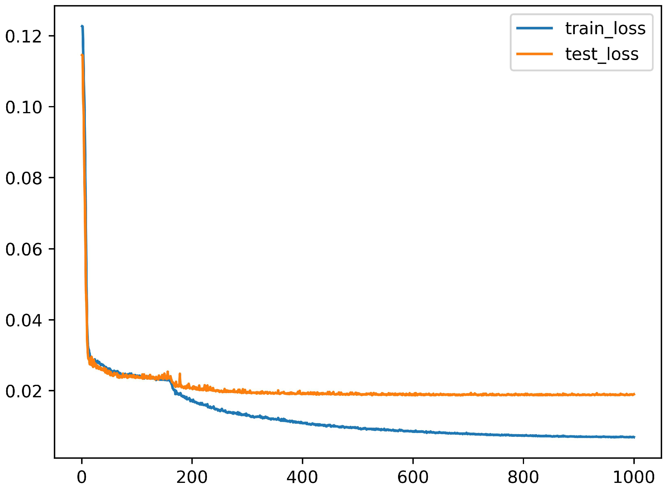
Figure 1. Training and validation loss over 1000 epochs. The training loss (blue) decreases rapidly and stabilizes near 0.10, while the validation loss (orange) converges around 0.15 ± 0.02 , indicating stable convergence and controlled generalization error.
Aerospace 12 00842 g001
Figure 2. Reconstruction of 300 hPa U and V wind components at 12:00 UTC on 1 February 2022.
Aerospace 12 00842 g002
Figure 3. Comparison of reconstructed wind fields. The green areas indicate locations with available observations. (a) Reconstructed wind field. (b) Ground-truth wind field.
Aerospace 12 00842 g003
Figure 4. Wind field reconstruction results under more complex conditions.
Aerospace 12 00842 g004
Figure 5. Wind field reconstruction errors across pressure levels. The x-axis spans from 50 to 800 hPa (approx. 20,000–2000 m, 65,000–6500 ft). The blue region indicates typical cruising altitudes for civil aviation (5400–11,300 m/18,000–37,000 ft, 475–225 hPa). The pressure–altitude conversion is inherently non-linear and is derived from the International Standard Atmosphere (ISA).
Aerospace 12 00842 g005
Figure 6. Relationship between MAE and spatial distance. The (a) shows wind speed MAE, while the (b) presents wind direction MAE. Both use box plots across different distance intervals to reflect distribution and variation.
Aerospace 12 00842 g006
Table 1. Performance evaluation of QMW-Net on wind field reconstruction at the 300 hPa pressure level in 2021.
NetTargetMAEMRERMSER2
QMWSpeed (m/s)1.626.68%2.580.93
Direction (degree) 14.8529.80.82
1 A higher R 2 value indicates better predictive performance of the network. The MRE value for wind direction is omitted because it only reflects the effect of normalization; a dash is used as a placeholder.
Table 2. Comparison of MAE in wind speed and direction between QMW and PINN models. The Total column indicates the average error across all listed dates.
NetTarget01/0102/0103/0104/0105/0106/0107/0108/0109/0110/01Total
QMWSpeed (m/s)1.970.891.401.952.981.181.654.052.503.602.20
Direction (degree)3.254.503.302.6015.807.4012.5010.803.854.956.90
PINNSpeed (m/s)2.762.742.622.513.203.363.182.843.102.342.87
Direction (degree)9.204.305.703.003.604.6024.5018.9026.0017.0011.68
Table 3. Comparison of wind speed and direction MAE between QMW and GPR models.
ModelMetric09/0109/1510/0110/1511/0111/1512/0112/15Total
QMWSpeed (m/s)1.261.242.211.581.020.894.381.421.73
Direction (degree)5.972.071.100.901.918.257.122.883.79
GPRSpeed (m/s)2.314.262.151.483.442.812.862.422.72
Direction (degree)25.334.392.253.932.204.495.392.947.62
Disclaimer/Publisher’s Note: The statements, opinions and data contained in all publications are solely those of the individual author(s) and contributor(s) and not of MDPI and/or the editor(s). MDPI and/or the editor(s) disclaim responsibility for any injury to people or property resulting from any ideas, methods, instructions or products referred to in the content.