Article

The BO-FCNN Inter-Satellite Link Prediction Method for Space Information Networks

Graduate School, Space Engineering University, Beijing 101416, China
*
Author to whom correspondence should be addressed.
Aerospace 2025, 12(9), 841; https://doi.org/10.3390/aerospace12090841
Submission received: 2 July 2025 / Revised: 5 September 2025 / Accepted: 5 September 2025 / Published: 18 September 2025
(This article belongs to the Section Astronautics & Space Science)

Abstract

With the rapid growth in satellite types and numbers in space information networks, accurate and fast inter-satellite link prediction has become a core requirement for topology modeling and capability evaluation. However, the current space information networks are characterized by large scales and the coexistence of multi-orbit satellites, posing dual challenges to inter-satellite link prediction. Link state prediction demands higher accuracy with limited computing power, while diverse satellite communication antenna loads require stronger generalization to adapt to different scenarios. To address these issues, this paper proposes a fully connected neural network model based on Bayesian optimization. By introducing a weighted loss function, the model effectively handles data imbalance in the link states. Combined with Bayesian optimization, the neural network hyperparameters and weighted loss function coefficients are fine-tuned, significantly improving the prediction accuracy and scene adaptability. Experimental results show that the BO-FCNN model exhibited an excellent performance on the test dataset, with an F1 score of 0.91 and an average accuracy of 93%. In addition, validation with actual satellite data from CelesTrak confirms the model’s real-world performance and its potential as a reliable solution for inter-satellite link prediction.

1. Introduction

A space information network is a complex system composed of the space segment (satellites and other spacecraft for communication, navigation, and remote sensing), the near-space segment (UAVs and other adjacent aircraft), and the ground segment (measurement and control points, information processing centers, users, etc.). Its key feature is the heterogeneity of the network elements, reflected in satellite orbit heights and functions. In recent years, the development of satellite constellations such as the Starlink constellation, the GW constellation, and the Thousand Sails constellation has steadily increased the number of satellites, further enhancing network heterogeneity. Unlike traditional satellite networks with fixed mesh topologies, such as Iridium [1] and Walker [2], where the inter-satellite links are relatively stable, space information networks comprise large-scale, diverse constellations with dynamic and intermittent inter-satellite links between satellites at different altitudes and inclinations. These characteristics complicate the network topology, making analysis and evaluation more challenging. Accurate satellite link prediction and dynamic topology construction are therefore essential. Conventional topology construction methods mainly rely on orbit simulation tools such as STK [3], NS-2 [4], and SGP4 [5], which propagate satellite states using two-line element (TLE-RRB) sets. While these methods provide accurate inter-satellite link states, large-scale network analysis will increasingly require rapid, iterative calculations of dynamic topologies across varying scales and configurations. Traditional link prediction approaches, however, demand significant computational power and long simulation times. Given diverse application scenarios, the topology analysis of space information networks must improve, particularly in terms of efficiency under limited computing resources. Therefore, developing an inter-satellite link prediction algorithm that requires low computing power, achieves fast calculation speeds, and maintains high prediction accuracy is essential.
As satellite network configurations have become more complex and space information networks expand in scale, inter-satellite link prediction has become a prominent topic in the field of satellite network topology. The authors of [6] employed predictive algorithms to learn and construct satellite contact windows. However, these algorithms rely on linearization simplifications in calculating encounter probabilities, limiting their application to specific orbital types and standardized constellation configurations. With the growing heterogeneity and size of satellite networks, efforts to model the temporal evolution of large-scale satellite connections in an autonomous and cost-effective way have advanced, aiming to better address the heterogeneity challenges in inter-satellite link prediction. To this end, supervised learning methods have been introduced to predict the link status between satellites, with fully connected neural networks (FCNNs) used to forecast inter-satellite links on circular and polar orbits [7]. This approach partially solves the problem of link prediction between heterogeneous satellites at the same altitude. Optimizing the FCNN also addresses the dataset imbalance caused by fewer links. However, the existing methods primarily optimize the weighted loss function during FCNN training without fully considering the network structure parameters or the weighted loss function settings. Neural network hyperparameter tuning methods are constantly emerging, such as the biological genetic algorithm [8] and hyper-heuristic algorithms [9]. In recent years, Bayesian optimization for neural networks has become a prominent research direction. Bayesian optimization has been applied successfully in predicting municipal waste generation, long-term water quality, and other neural network- and deep learning-based prediction tasks, demonstrating a strong temporal prediction performance [10,11,12,13,14]. In addition, the authors of [15] use a Bayesian-optimized convolutional neural network to address unbalanced data, aligning with the characteristics of inter-satellite link prediction data in space information networks discussed in this paper.
In summary, the traditional FCNN method shows potential for solving inter-satellite link prediction, but gaps remain in terms of its accuracy and generalization. Bayesian optimization is a powerful method for optimizing neural network architectures by efficiently tuning the hyperparameters to improve the model performance. It also demonstrates adaptability to dataset imbalance through adjustment of the loss function parameters. Therefore, this paper proposes an FCNN model combined with Bayesian optimization to optimize the number of network layers, the number of neurons in each layer, and the loss function parameters. Metrics such as the F1 score, recall, and balanced accuracy are used to evaluate the prediction accuracy for unbalanced datasets, and the influence of the classification thresholds on the prediction accuracy is analyzed. This approach addresses inter-satellite link prediction in space information networks and improves prediction performance.
The structure of this paper is as follows. Section 2 introduces the concept of space information networks, analyzes their topological characteristics, and defines the inter-satellite link prediction problem, highlighting its necessity, challenges, and potential solutions. Section 3 presents the proposed FCNN model based on Bayesian optimization, formulates the inter-satellite link prediction problem, and describes the construction of the training, verification, and test sets, as well as the evaluation criteria. In Section 4, the parameter optimization results are presented, and the prediction and generalization abilities of the BO-FCNN, FCNN, BP, LSTM, Random Forest, and other models are analyzed and compared. The impact of classification thresholds on the model performance is also examined, and the prediction effect is further verified using real satellite data from CelesTrak. Section 5 discusses the model approach, hyperparameter optimization, dataset imbalance, and computational cost. Finally, Section 6 summarizes the main findings and offers suggestions for further research in this field.

2. Inter-Satellite Link Prediction and Problem Analysis of Space Information Networks

2.1. Overview and Analysis of Space Information Networks

A space information network is a complex system composed of a satellite network and a terrestrial network. Since the ground network is relatively fixed, this paper focuses on the satellite network, which consists of large-scale satellite groups with diverse orbit types and functional characteristics. Its core function is to enable multi-functional, high-speed, and large-capacity information acquisition and transmission by integrating satellites such as GEO, MEO, and LEO satellites. This integration allows for multi-dimensional information collection and transfer, providing global coverage, high reliability, and flexible services. As shown in Figure 1, the space information network can be divided into high-, medium-, and low-orbit layers, each containing functional satellites, including communication, early-warning, navigation, and reconnaissance satellites, based on their capabilities. Cross-layer and cross-domain information transmission is achieved through inter-satellite links, improving the overall efficiency of the network.
The topological structure characteristics of space information networks are summarized as follows:
(1) Large number and scale
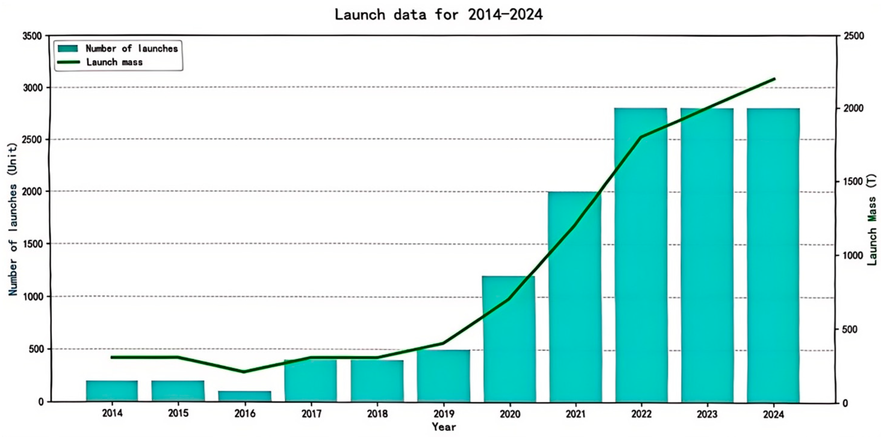
The network’s member nodes include satellite platforms with reconnaissance, early-warning, navigation, and communication functions at various orbital altitudes, as well as information transmission platforms, such as ground stations. These heterogeneous nodes form an interconnection network with diverse standards and functions. According to the Global Launch Statistics Report [16] (Figure 2), the number of satellites launched in 2024 increased dramatically compared to that in 2014. The large number of nodes further increases the complexity of the network topology.
(2) Complex network structure
Due to the network’s large scale and variety of subsystems, interactions are frequent, and coordination is complex. Satellites of different types and functions must establish stable links, which increases topological complexity. Satellites’ differing functions and operational requirements result in variations in their orbital altitudes, orbit shapes, and other parameters.
(3) Highly time-varying topology
The network consists of numerous satellite and ground platforms. Satellite platforms move at high speeds around the Earth with predictable orbital patterns, but the relative positions and links between platforms change continuously, causing constant changes in the network topology.

2.2. Inter-Satellite Links

Inter-satellite link prediction in a space information network aims to predict the link status between any two satellites over a future period. The link status is expressed as x { 0 , 1 } , where 0 indicates no link and 1 indicates a link. The basic satellite parameters include the six orbital elements and the communication antenna parameters.
(1) Basic parameters of satellites
Orbital elements uniquely define a satellite’s orbit in terms of shape, size, and orientation. There are six elements: the semi-major axis (a); the distance from the Earth’s center to apogee; the eccentricity (e); the deviation of the orbit from a circle; the inclination (i); the angle between the orbital plane and the reference plane. The right ascension of the ascending node (Ω) is the angle between the vernal equinox and the ascending node, which specifies the orientation of the orbital plane relative to the Earth’s equatorial plane. The argument of periapsis (ω) is the angle between the eccentricity vector and the ascending node. The true perigee angle ( φ ) is the angle between the eccentricity and the satellite’s position vector and is used to determine the satellite’s location along its orbit. Since this paper primarily considers satellites in circular orbits, the eccentricity is zero, and the semi-major axis equals the sum of the orbital altitude and the Earth’s radius. The ranges of the remaining parameters are given in Table 1.
(2) Antenna load parameters
(a) Communication distance
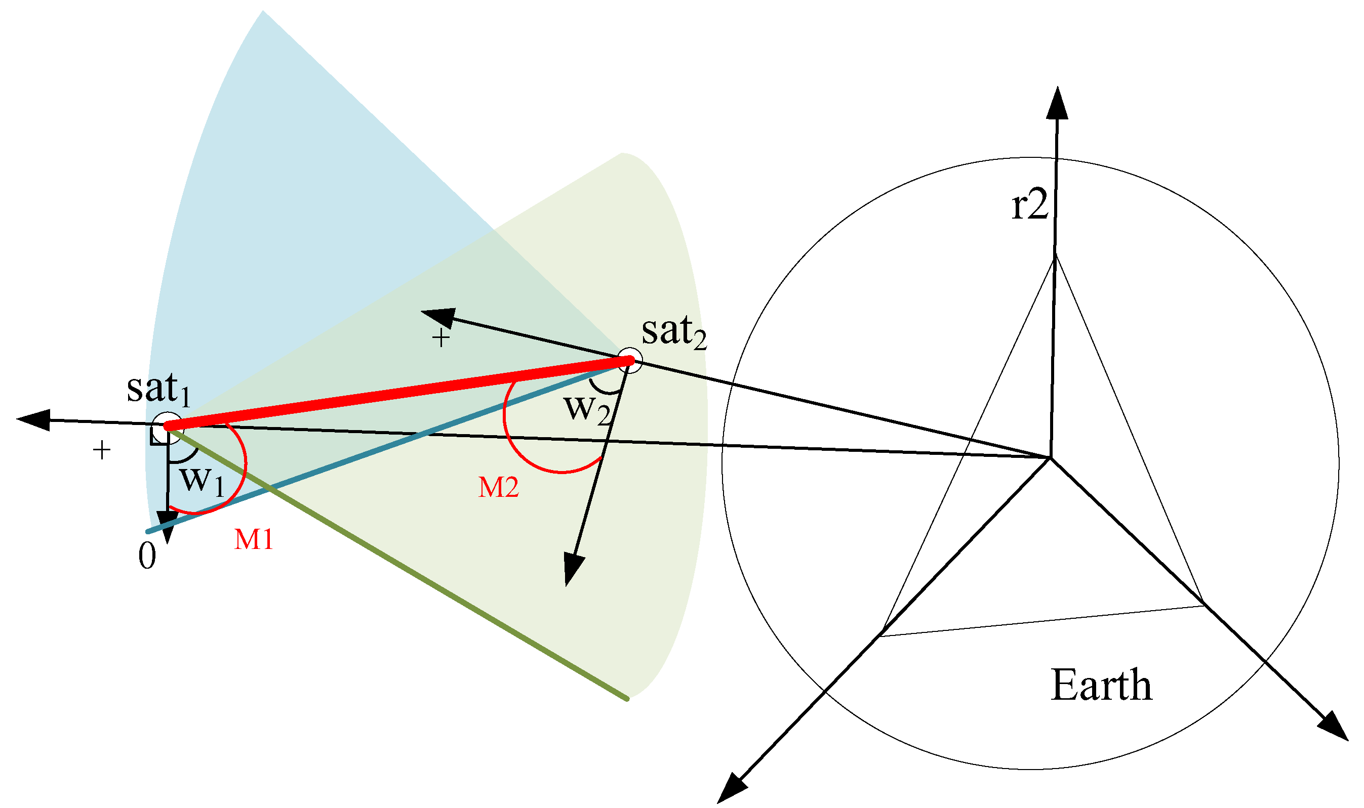
According to [7], without considering detailed antenna-pointing processes, a link exists between satellites when the Euclidean distance between them is below a given threshold, and each directional antenna is equipped with a pointing mechanism. To capture inter-layer interactions in a space information network, this paper focuses on inter-satellite links in different orbital layers, e.g., LEO to MEO and MEO to GEO. Typically, the communication distance from LEO to MEO is approximately 10,000 km. Assuming the communication distance is W, the distance between satellites is L, the satellite’s semi-major axis is R, and the Earth’s radius is R, links are shown in Figure 3.
The possibility of a link is determined by the distance between satellites. As shown in Figure 3a, both Satellite 1 and Satellite 2 are in circular orbits, with semi-major axes (r1 and r2) and maximum communication distances (W1 and W2), respectively. Let L be the distance between the two satellites, h the distance from the line connecting them to the Earth’s center, and R the Earth’s radius. A two-way communication link is possible if L is within both satellites’ maximum communication distances and h is greater than R:
p = L + r 1 + r 2 2 h = p ( p L ) ( p r 1 ) ( p r 2 ) x = 1 L < W 1 L < W 2 h > R 0 L > W 1 L > W 2 h < R
(b) Antenna directivity
Establishing inter-satellite links also depends on antenna orientation. This paper focuses on inter-satellite links at different orbital altitudes, so the elevation angle of the antenna is introduced. Assuming the orbital altitude of Satellite 1 is higher than that of Satellite 2, the azimuth angle of the antenna ranges from 0 to 360°. The elevation angle ranges are (W1, −180 − W1) for Satellite 1 and (W2, 180 − W2) for Satellite 2, as shown in Figure 4. Let M1 and M2 be the angles of the line connecting the satellites relative to the pitch angles of Satellites 1 and 2, respectively. When M1 and M2 fall within the respective pitch angle ranges, the two are considered linkable.
As shown in Figure 4, when both satellites are within each other’s pitch angle ranges, a link between them is possible. This possibility is denoted as y, where y = 1 indicates that the pitch angle satisfies the link condition, and y ≠ 1 indicates that it does not. The formula is as follows:
y = 0 M 1 < 180 W 1 M 1 > W 1 M 2 < W 2 M 2 > 180 W 2 1 W 1 > M 1 > 180 W 1 W 2 < M 2 < 180 W 2
In summary, when both X and Y equal 1, an inter-satellite link is established between the satellite pair.

2.3. Summary

In summary, the current space information networks face major challenges: large scales, complex compositions, and strong time variability. These factors present two difficulties for inter-satellite link prediction. First, the large number of satellites creates heavy computational demands for inter-satellite link simulations. Traditional simulation tools such as SGP4 and STK can accurately determine satellite orbits and calculate link conditions using the six orbital elements. However, with limited computing power, they cannot efficiently handle large-scale network simulations. Supervised learning methods have achieved high accuracy and are widely applied to large-scale networks. Nonetheless, further optimization of the hyperparameter and loss function selection in the FCNN structure could improve accuracy. Second, because satellites differ in their orbital shapes and altitudes, the completeness of data samples must be considered when constructing inter-satellite link prediction models. The existing studies often focus only on the antenna properties, mainly the communication distance threshold, while paying insufficient attention to the azimuth and elevation angles. Therefore, this paper aims to optimize model design by improving the antenna parameter coverage, algorithm fit to data samples, and overall prediction accuracy.

3. Inter-Satellite Link Prediction Model Based on Bayesian Optimization

3.1. Theory

3.1.1. Bayesian Optimization

Bayesian optimization (BO) is a global optimization strategy based on a probabilistic model. It is mainly used to optimize highly nonlinear, nonconvex objective functions without analytical gradient information [17]. BO combines Bayesian inference and probabilistic modeling to construct the posterior distribution of the objective function and uses this distribution to guide the search process toward an approximate optimal solution. Bayesian optimization typically employs a Gaussian process as its surrogate model to predict the function values and associated uncertainty in unexplored regions. The formula is as follows:
f ( x ) ~ G P ( m ( x ) , k ( x , x ) )
A Gaussian process is a stochastic process with a multivariate normal distribution. Gaussian process regression fits the objective function (f(x)) as the surrogate model. The acquisition function then determines the next exploration point based on predictions from the current surrogate model to optimize the objective function. Common acquisition functions include expected improvement, probability of improvement, and greedy descent. The expected improvement function is expressed as
E I ( x ) = ( f ( x + ) μ ( x ) ) Φ ( Z ) + σ ( x ) ϕ ( Z ) ,
where Z = f ( x + ) μ ( x ) σ ( x ) .
In the formula, E I ( x ) is the expected sampling function; x + is the currently known optimal input; f ( x + ) is the currently observed optimal objective value; μ ( x ) and σ ( x ) are the predicted mean and standard deviation of the surrogate model at point x , respectively; Φ and ϕ are the cumulative distribution function and probability density function of the normal distribution; and Z is the normalized score representing the magnitude of improvement relative to the best observed value. When Z is greater than 0, the predicted improvement is positive, indicating that the model’s performance at this point is expected to exceed the currently known best performance.

3.1.2. FCNN Model

An FCNN consists of an input layer, multiple hidden layers, and an output layer. Each neuron in a layer connects to all neurons in the preceding layer. Through linear transformations and nonlinear activation functions, the FCNN extracts input features and maps them to the output space. The input layer receives data, the hidden layers capture complex patterns through nonlinear transformations, and the output layer generates results. The network updates its weights using backpropagation [18].

3.2. Inter-Satellite Link Prediction Model Framework

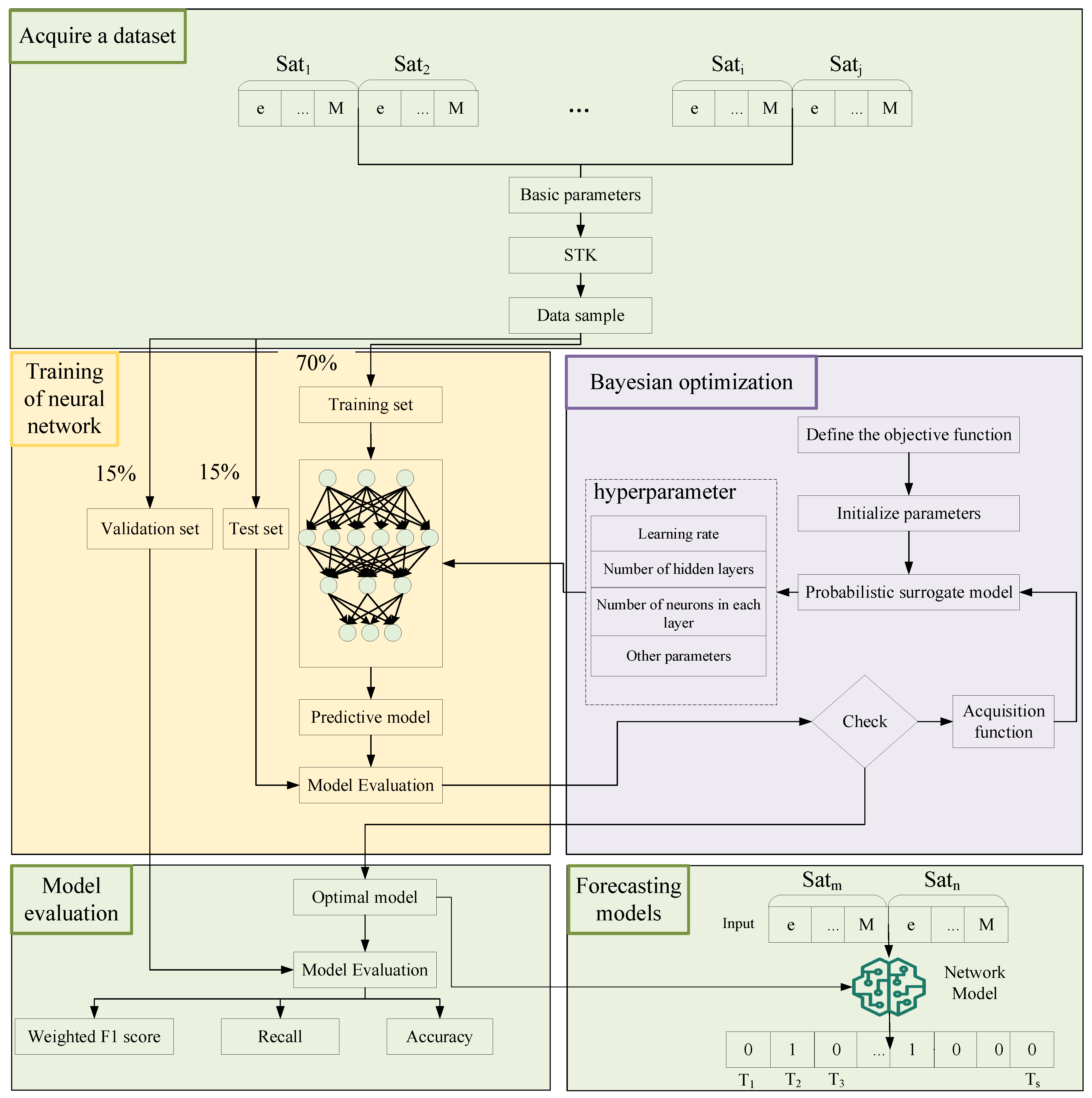
Inter-satellite links between satellite pairs in space information networks are the focus of this paper. To achieve accurate prediction for any satellite pair, we propose an inter-satellite link prediction algorithm that addresses the large sample size and imbalance of the link states. The proposed BO-FCNN model integrates Bayesian optimization with an FCNN. The former optimizes the hyperparameter configuration and other settings of the FCNN, while the latter extracts state features of the inter-satellite link from the data. This approach enhances performance, particularly when handling limited or imbalanced samples. The BO-FCNN model consists of two main components, and its workflow is illustrated in Figure 5.

3.2.1. Data Partitioning and Pretreatment

Based on the analysis of the space information network structure in Section 2 and the basic parameter settings and link definitions of inter-satellite links, the parameter ranges in Table 1 were used to generate 20 W satellite-pair datasets through STK and MATLAB 2024a co-simulation. The data were divided into 70% for training, 15% for testing, and 15% for validation. In addition, orbital data for 200 real LEO satellites and 30 real MEO satellites were obtained from CelesTrak as a control group, with the orbital parameters constrained to the ranges in Table 2.
The data used in this paper comes from the composite data obtained by STK. The composite satellite data depends on the six elements of the satellite orbit. The orbit calculation uses a J2000 inertial frame of reference, the data timestamp is uniform UTC time, the SGP4/SDP4 orbit model is used to calculate the orbit data of the synthetic satellite, and the accurate and available dataset of the inter-satellite link is obtained. In the field of inter-satellite link analysis [19,20,21], this method is used in the literature to obtain synthetic data, so the dataset is reliable, effective, and referential.
The input training data consist of combinations of medium- and low-orbit satellites at circular orbits at altitudes of 1000 km and 10,000 km. Satellite pairs (SO1–ST1) were defined by randomly generating six orbital elements. The input training data are listed in Table 2. For this study, satellites were assumed to be in circular orbit with eccentricity (E) = 0. Two preprocessing steps were performed before fitting the input data into the model:
(a) All orbital parameter values were randomized to generate a more realistic, non-uniform distribution (see reference table);
(b) All orbital parameter values were normalized to a range of −2 to 2 to balance the importance of the input features.
The dataset is shown in Table 3. Since this study focused on inter-satellite link state prediction at fixed orbital altitudes, the semi-major axis (A) was not included in the normalization process.
In this paper, the min–max scaling method was used to normalize the data. The formula is
X N = X X min X max X min
In the formula, X is the original value; X N is the normalized value; X min is the minimum value; and X max is the maximum value. The normalized dataset is shown in Table 4.
The output training data consist of the link states of satellite pairs. The input training set, generated by STK, spans the next 24 h at 5 min intervals. Each link state is defined as 0/1, forming a 1 × 288 time series vector. The output training data comprise 20 W of such vectors. Examples are shown in Table 5.

3.2.2. Definition of the Loss Function

Analysis of the inter-satellite link shows that the link and non-link states are highly imbalanced, posing a challenge for model training. To address this imbalance, The following Equation defines the weighted loss function (L) used for training. This loss function has been shown in the literature to outperform default functions such as the mean-square error [22], the mean absolute error [23], and cross-entropy [24]:
L = ( A Y t + 1 ) ( Y t Y p ) 2
where Y t is the true value, Y p is the predicted value, and a is a positive constant. The literature indicates that performance is optimal when a is less than 1. For more imbalanced datasets, a larger a may be required. Because the degree of imbalance varies across samples, the value of a also changes. Therefore, this paper incorporates a into the optimized hyperparameters to improve the training performance for the current dataset and provide guidance for more complex data.

3.2.3. Model Parameter Settings

Each neural network layer applies an activation function to its output to introduce nonlinearity, enabling the model to learn more complex representations of its inputs. The input layer contains 14 neurons, and the output layer contains 288 neurons. The hidden layer uses the rectified linear unit activation function, while the output layer uses the sigmoid function to produce values between 0 and 1, representing the link state. Training was performed for 500 batches of 3000 samples each, using the BO-FCNN model with a custom loss function, the Adam optimizer, and an early-stopping patience of 200 to avoid overfitting. Given the large sample size and pronounced imbalance, the number of hidden layers (m), the number of neurons (N) in each layer, the learning rate (E), and the parameter (a) in the custom loss function (L) were optimized. The initialization and optimization ranges are shown in Table 6.

3.2.4. Model Training

The BO-FCNN model was trained as follows:
(a) Objective function on an imbalanced dataset: The FCNN model was evaluated using an objective function. The optimization objective was the F1 score (see point (5)).
(b) Hyperparameter space: The hyperparameter space of the FCNN was established, and BO was used to search it efficiently. The hyperparameters included the number of hidden layers, the number of neurons in each layer, the learning rate, and a, defined as
Φ = { m , n , e , A }
(c) Bayesian optimization
BO progressively searched for the best hyperparameter combination and modeled the hyperparameter space using a GP. Given θ t as the current hyperparameter combination, BO selected a new hyperparameter ( θ t + 1 ) by maximizing the objective function with surrogate model evaluation. BO aimed to identify the optimal hyperparameters by increasing the surrogate model’s expected value ( f ( θ ) ):
θ t + 1 = arg max θ f ( θ )
(d) Grid search
BO automatically adjusted the hyperparameter configuration of the CNN to improve the model performance. By evaluating each configuration on the validation set, the optimization process updated and maintained the current best hyperparameter state. The BO iterative update process is
θ t + 1 = θ + Δ θ
(e) FCNN model training
The FCNN model was trained using the hyperparameters tuned by BO, thereby improving the performance on imbalanced data.

3.2.5. Performance Evaluation

Because the dataset was imbalanced and the output was a binary classification (0, 1), the proposed BO-FCNN inter-satellite link prediction model was evaluated using four indices: the accuracy (ACC), precision, recall, and F1 score:
A C C = T P + T N T P + F P + T N + F N
Pr e c i s i o n = T P T P + F P
Re c a l l = T P T P + F N
F 1 s c o r e = 2 Pr e c i s i o n Re c a l l Re c a l l + Pr e c i s i o n
Here, TP denotes true positive, where the true class is correctly predicted as true; TN denotes true negative, where the true class is correctly predicted as false; FP denotes false positive, where the false class is predicted as true; and FN denotes false negative, where the false class is predicted as false. TPs, TNs, FPs, and FNs form the confusion matrix (Table 7), which was used to calculate the prediction results.
(a) Accuracy
The accuracy is the proportion of samples predicted as positive that are truly positive. It is suitable for cases where misclassifying negative samples as positive incurs a high cost.
(b) Recall
The recall is the proportion of true positives correctly predicted. It is suitable for cases where missing positive samples carries a high cost.
(c) F1 score
The F1 score is the harmonic mean of the precision and recall, reflecting the balance between them. It is suitable for imbalanced samples where both FPs and FNs must be considered.
Given the imbalance in this dataset, the precision, recall, and F1 score were emphasized when evaluating the prediction model. During model optimization, the F1 score was also used as the objective function to ensure balanced evaluation and improve the prediction accuracy.

4. Results

This section presents the performance of the BO-FCNN model architecture described in Section 3. First, the optimal parameter selection obtained from the Bayesian-optimized FCNN model is reported. Then, the performances of the BO-FCNN and FCNN models are compared using indicators such as the F1 score, recall, and precision. Then, through threshold analysis, the best score classification threshold is determined. Finally, the prediction effect is further verified using real satellite data from CelesTrak.

4.1. Parameter Optimization

Based on the model parameter settings in Section 3.1, Bayesian optimization was used to tune the hyperparameters {m, n, e, a}. The parameter ranges are shown in the table. The number of initialization points was set to 5, and the number of iterations was 25. The objective function was the average F1 score.
As shown in Figure 6, as the number of iterations increased, the average F1 score rose sharply. After 12 iterations, the average F1 score gradually stabilized, fluctuating around 0.9. At this point, the model was considered optimal; the corresponding optimal hyperparameters are shown in Table 8.

4.2. Control Trial

In this section, we report comparative experiments performed on the BO-FCNN model. Because the dataset distribution and communication thresholds vary, their influences on the dataset characteristics also differ. For comparison, the FCNN model follows the neural network parameter settings in [7], uses the dataset provided in this paper, and is evaluated against the BO-FCNN model. The results show that the Bayesian optimization method performs well in optimizing the neural network structure for this problem and can effectively improve the applicability of the FCNN model in inter-satellite link prediction. To comprehensively evaluate the advantages and disadvantages of the BO-FCNN model, additional models commonly used in classification and prediction—such as BP neural networks, Random Forest, and LSTM—are also included in the comparative analysis.
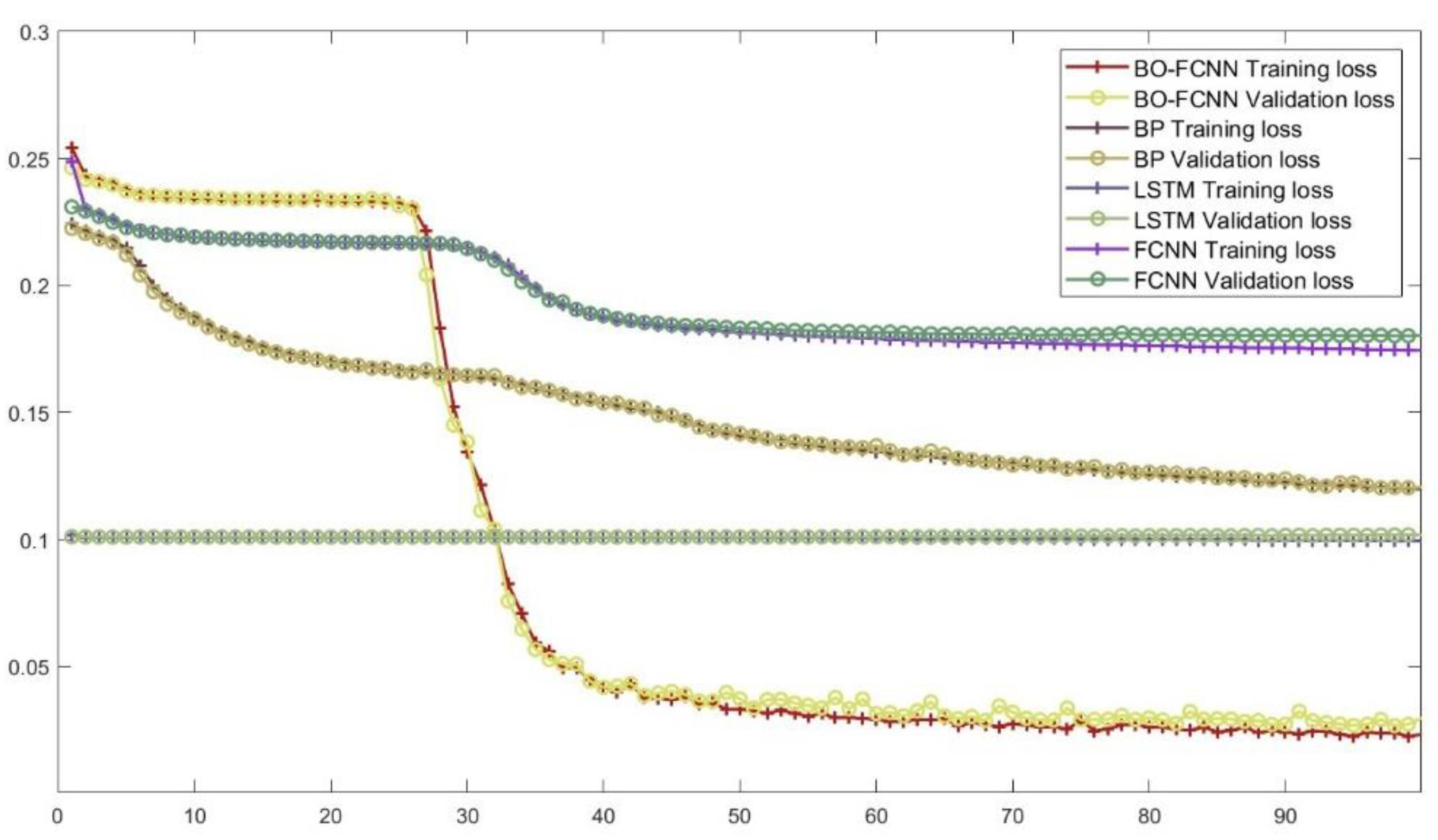
The baseline FCNN model, as defined in [7], was configured with the following parameters: a total of 14 neurons in the input layer, 576 neurons in the output layer, and four hidden layers, with 32, 64, 128, and 256 neurons, respectively. This configuration contained a total of 279,488 trainable parameters for minimizing the loss function. Although this configuration performed well on the dataset from the referenced literature, it cannot be directly applied to inter-satellite links with different antenna parameters. To ensure a fair comparison across models—including the FCNN, the BO-FCNN, BP neural networks, and LSTM—a custom loss function was used in this paper. The dataset established in this paper was used to compare these models by analyzing their loss functions and the accuracy changes over iterations.
As shown in Figure 7, the LSTM method did not perform well on datasets with severe class imbalance but was more effective for problems with temporal periodicity between data samples. The BO-FCNN, FCNN, and BP models all showed downward trends in their loss values. Among them, the FCNN and BO-FCNN stabilized after a certain number of iterations, indicating that their prediction models were relatively reliable. The similar trends of training and verification losses indicate a stronger generalization ability, while the BO-FCNN showed clear advantages in reducing loss from the same starting point. Although the BP model also showed a downward trend, which was better than the traditional FCNN model, it did not converge to a stable state. This instability, related to model convergence, indicates the difficulty in prediction under extreme data imbalance.
To more accurately evaluate the performance differences among the algorithms, each prediction model was analyzed using the average F1 score, average recall, average precision, training time, and other indicators. The results are shown in Table 9.
The BO-FCNN performed well in terms of the average F1 score, recall, and precision. However, due to hyperparameter optimization, its training time was longer. Random Forest and LSTM were not suitable for datasets with extreme imbalance. The BP model outperformed the traditional FCNN on the performance metrics but lacked stability. Overall, the BO-FCNN showed strong results in both the performance metrics and model stability, as its hyperparameter optimizations allowed it to adapt to different imbalanced datasets.

4.3. Threshold Analysis for Classification

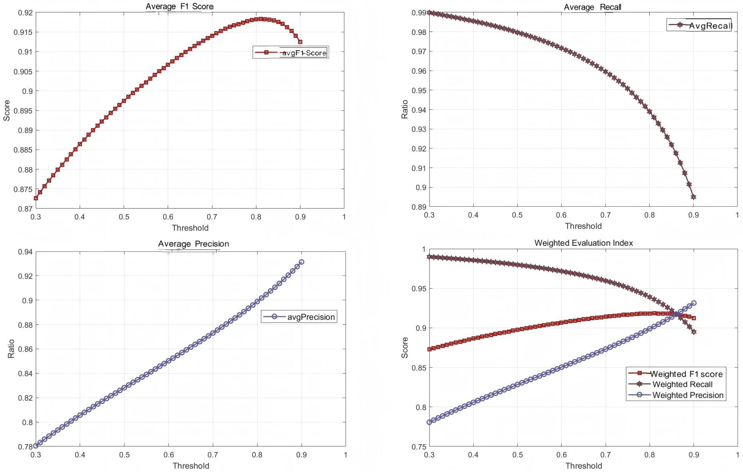
Because the BO-FCNN model uses a classification threshold to divide prediction outputs into 0 and 1 in the prediction process, variations in the threshold significantly affect the evaluation metrics of the final prediction model. In this paper, the classification threshold was analyzed to determine the optimal value of the classification threshold. The probability was set from 0.3 to 1 with a step size of 0.01, and the results are shown in Figure 8.
The average recall showed a gradual downward trend, while the precision increased, reflecting the inherent trade-off between the two. The average F1 score increased with the classification threshold until it reached 0.8. The optimal average F1 score, recall, precision, and corresponding classification threshold are presented in Table 10. Since the dataset used in this paper contained 288 output dimensions, the classification threshold analysis required higher accuracy to obtain reliable performance metrics. A weighted-index method was therefore applied: each dimension was calculated separately and then combined into a weighted sum according to the index weights. The resulting weighted F1 score, recall, and precision followed the same trend as that of the final optimal classification threshold, indicating consistency in the output-dimension weights.

4.4. Case Studies

To verify the accuracy of the BO-FCNN model and its applicability to real satellite data, the satellite data in Table 11 were used to form 6000 sets of satellite pairs as the verification set. The trained BO-FCNN model was then evaluated on this set, and its performance metrics are shown in Table 11.
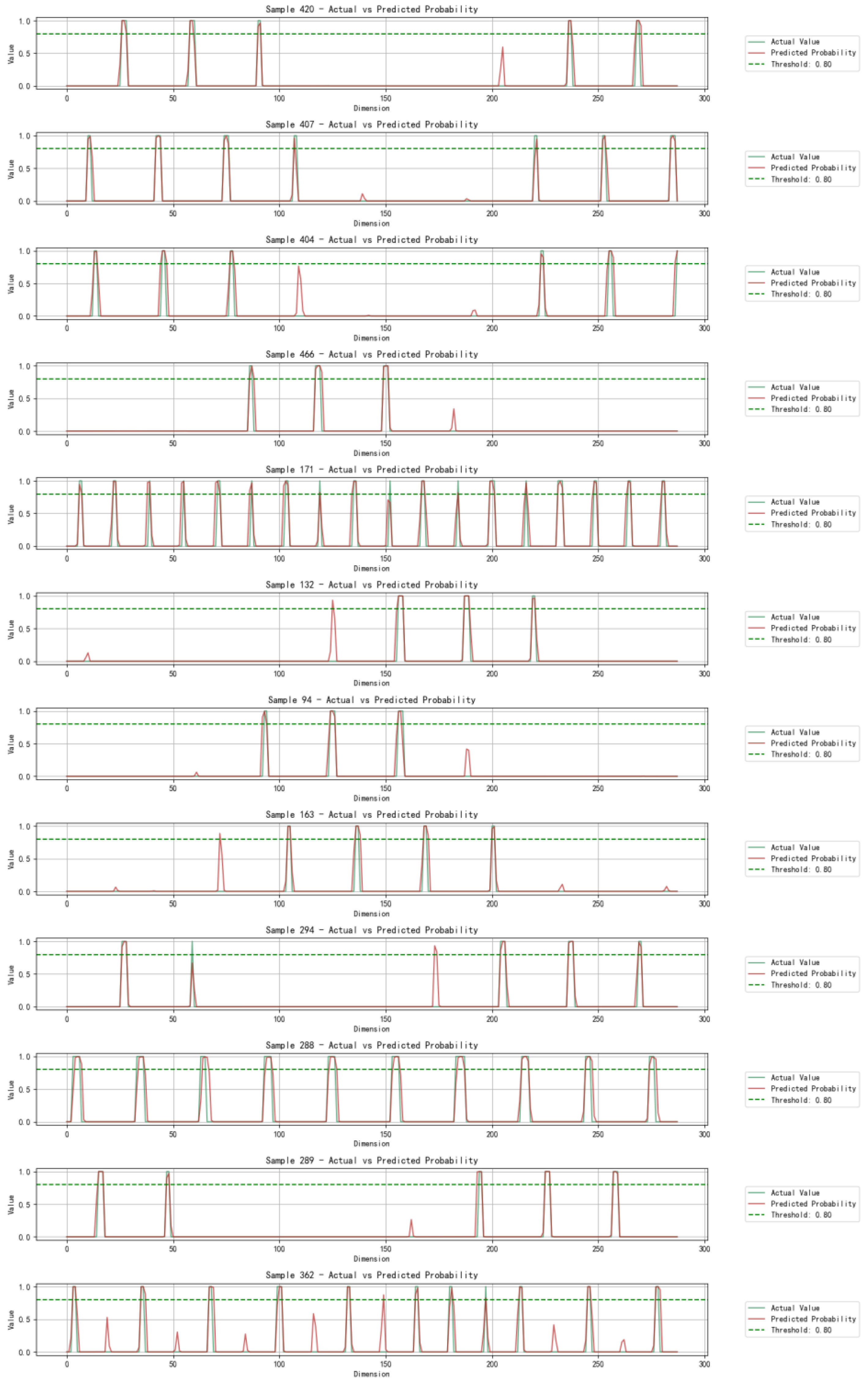
To provide a more intuitive assessment, 12 satellite pairs were randomly selected from the validation set for visual analysis. In the plots, the green, solid lines represent the real connection states, the red, solid lines represent the predicted probabilities, and the green, dotted lines represent the classification thresholds. If the probability exceeds the classification threshold, a connection is predicted; otherwise, no connection is predicted. As shown in Figure 9, the 12 satellite pairs were predicted accurately.

5. Discussion and Analysis

To further explore the problem of inter-satellite link prediction, this section analyzes the BO-FCNN prediction model from four aspects: ablation test, optimization parameters, dataset imbalance, and computational cost. These analyses demonstrate the model’s advantages and identify directions for further improvement.

5.1. Model and Parameter Analysis

5.1.1. Model Analysis

(1) Model comparison
In order to verify the performance improvement effect of Bayesian optimization (BO) on the FCNN, the suitability of BO in the time dimension was explored, and the F1 score, recall, precision, and hyperparameter search time were used for analysis. The establishment of the experimental group is shown in Table 12.
The dataset in this paper was used for training, and the purpose of this experiment was to analyze the model method. Therefore, in order to save the computational cost, a fixed learning rate was selected, and only the number of hidden layers and the number of neurons in each layer were considered. The eigenvalue (A), optimization range (reference Table 6), and performance index + hyperparameter search efficiency of five sets of experiments were obtained, as shown in the Table 13.
The following conclusions can be drawn from the ablation contrast test.
First, Bayesian optimization is the key to break through the performance bottleneck of the FCNN in the field of inter-satellite link prediction: it can be found that the F1, F2, and F3 methods with parameter optimization have better performances in terms of the average F1 score, average recall rate, and average precision rate. In addition, by comparing F3 with F1 and F2, it can be found that the optimization effect of Bayesian optimization is significantly higher than that of F1 and F2. In terms of the hyperparameter search time, although F3 is not as fast as F1, it is significantly faster than F2 and at a medium level.
Secondly, there is a synergistic effect of 1 + 1 > 2 between Bayesian optimization and time-varying modeling: by adding the BO-FCNN method to the traditional LSTM method, its prediction effect is significantly improved compared with the traditional LSTM method. Therefore, the introduction of time series modeling for inter-satellite link prediction plays a positive role. In the follow-up study, we will consider the performance of the BO-FCNN method in time series.
(2) Model stability analysis
K-fold cross-validation is used to eliminate the random bias caused by a single data partition and to quantify the robustness of the BO-FCNN model in the inter-satellite link prediction process through multiple rounds of the iterative validation of the data distribution. The specific implementation process includes data stratification, iterative verification, and result aggregation. Firstly, the dataset to be verified is randomly divided into k subsets of equal size according to the principle of non-overlap (in this paper, K = 5, where the K-1 subset is used as the training set, and the remaining one subset is used as an independent verification set). Then, in each round of verification, the Bayesian optimization module is used to dynamically search the optimal hyperparameter combination of the FCNN. After completing the training of the FCNN model based on the training set, the F1 score is obtained. The process is repeated k times to ensure that each subset is used as a verification set once, and finally, K sets of independent model performance data are obtained.
By calculating the average F1 score and RMSE, the standard deviation (reflecting the performance fluctuation range), and the coefficient of variation (CV) of the index, if the dispersion degree of the index is lower than the preset threshold (e.g., the coefficient of variation is less than 15%), it shows that the performance of the BO-FCNN method is consistent under different data distributions, the grid search process is not disturbed by the significant differences in data partitioning, and the model has a stable generalization ability. This method can make full use of the limited dataset and avoid the chance of traditional single verification, which provides a basis for the stability of the BO-FCNN method in inter-satellite link prediction.
Using the dataset of this paper, the stability of the BO-FCNN inter-satellite link prediction method proposed in this paper was verified by the k-fold cross-validation method, and the results are shown in Table 14 below.
Through the calculation of the coefficient of variation (CV) of the average F1 score and RMSE, it is found that both are less than 15%, which indicates that the fluctuation range of the average F1 score and RMSE is smaller than its mean proportion, the grid search process of the BO-FCNN is not significantly disturbed by the difference in data partitioning, and the prediction accuracy of the model under different data distributions is consistent and stable.

5.1.2. Parametric Analysis

The hyperparameters optimized in this study included the number of hidden layers (M), the number of neurons in each layer (N), the learning rate (E), and the loss function weight (a). Each hyperparameter was analyzed using the control variable method with respect to the F1 score, recall, and precision, as shown in Figure 10.
The number of hidden layers fluctuated significantly as M increased, indicating that selecting an appropriate number of layers was more important than simply increasing them. The number of neurons per layer showed a steady increase and stabilized once N reached a certain level, suggesting that the model could adequately capture the dataset’s characteristics. An increase in the learning rate initially improved the performance but caused fluctuations in the middle and later stages. This behavior reflected the trade-off between optimization efficiency and parameter space exploration, highlighting the need to set appropriate thresholds. The loss function weight (a) first improved the performance and then led to a gradual decline. This was due to the varying degrees of dataset imbalance, resulting in different requirements for A. Therefore, it is necessary to adjust A flexibly across different imbalance levels to ensure better adaptation to dataset characteristics.

5.2. Analysis of Dataset Imbalance

In [15], the authors point out that the scope and volume of data are increasing due to rapid advances in data science and machine learning. However, many real-world datasets—especially those related to classification problems—exhibit extreme class imbalance. Traditional machine learning methods often struggle with imbalanced data [22], producing poor predictions for certain classes. The same challenge also arises in the inter-satellite link prediction task considered in this paper. Both the antenna elevation (pitch) angle and the antenna communication distance affect the imbalance of the link-state labels in the dataset, which, in turn, affects the model performance. Therefore, this section analyzes how these two factors influence dataset imbalance and the final model’s performance, establishing a foundation for more complex prediction scenarios.
(1) Antenna-pointing parameter
At a fixed communication distance of 11,000 km, we consider two cases based on whether the antenna elevation angle is considered. For a sample satellite pair, we count the connected and non-connected states, as shown in Figure 11.
The antenna-pointing parameter substantially reduced the number of connected states compared with considering only the communication distance, thereby increasing the dataset imbalance. To more intuitively illustrate how this imbalance affects the model performance, we constructed two datasets: dataset A (Case 1), which used only the communication distance, and dataset B (Case 2), which also included the antenna elevation angle. We trained the BO-FCNN prediction model on both datasets.
Figure 12 shows the optimization curves for dataset A (red) and dataset B (yellow-green). The model achieved an acceptable performance without optimization; however, when the imbalance was severe, a small number of optimization iterations yielded improved results. Thus, the BO-FCNN adapts to different data characteristics caused by varying pointing parameters and improves through optimization. The performance metrics are shown in Table 15.
(2) Communication distance
To further analyze the algorithm’s sensitivity to dataset imbalance, we varied the antenna communication distance from 11,000 km to 9000 km and constructed seven datasets at intermediate distances. As shown in Figure 13, ayess the communication distance decreased, the number of connection opportunities dropped progressively; by 9000 km, inter-satellite links were nearly impossible. These datasets thus captured a wide range of class imbalance.
We applied the BO-FCNN prediction model to each dataset. The optimization process is shown in Figure 14, and the final optimization results are presented in Table 16.
As the communication distance decreased and the dataset imbalance increased, the BO-FCNN required more optimization iterations and attained progressively worse optimal results, eventually failing to optimize effectively. Analysis of the optimal hyperparameters across distances showed that for distances greater than 9750 km, the BO-FCNN model predicted effectively and yielded a better performance; the characteristic parameter (a) increased gradually. For distances below 9500 km, the prediction deteriorated markedly and ultimately failed due to extreme class imbalance. The hyperparameters trended upward prior to failure; given the current upper bound of 5 for the optimized parameter range, this suggests a practical optimal range for these parameters. Future work could increase the upper bound for parameter a (and other hyperparameters) or redesign the loss function to better accommodate extreme class imbalance.

5.3. Analysis of Computational Cost

To compare the computational cost of the trained BO-FCNN model with those of the traditional SGP4 and STK simulation tools, experiments were conducted on a computer with 32 GB of memory and a 13th Gen Intel (R) Core (TM) i5-13600KF processor. Under identical computing conditions, 200 satellite pairs were simulated to obtain their inter-satellite links. SGP4 required 2.3 s, STK required 244 s, and the BO-FCNN model required only 0.66 s—approximately three times faster than SGP4 and 369 times faster than STK. Thus, as the number of satellites increases in large-scale satellite networks, the computational cost can be greatly reduced. This demonstrates the model’s effectiveness in scenarios with limited computing power and high timeliness requirements, supporting efficient topology analysis and evaluation of large-scale satellite networks.

6. Conclusions and Future Directions

This paper proposes an FCNN-based model optimized with Bayesian methods to predict the establishment of inter-satellite links in space information networks. This method effectively predicts inter-satellite connectivity and provides a foundation for analyzing the topologies of future large-scale space information networks. The model uses the six orbital elements of a satellite pair as eight-dimensional input features and outputs a 24 h time series describing communication opportunities for satellites, including remote sensing and communications satellites. Using the STK simulation platform, we generated a random dataset of 200,000 satellite pairs (LEO at 1000 km and MEO at 10,000 km). The Bayesian optimization method was then applied to tune the hyperparameters (number of hidden layers, number of neurons per layer, learning rate, and weighted loss function (a)). The results show that the proposed method improves the FCNN performance, with the objective function defined as the average F1 score. The dataset was divided into training, validation, and test sets, and the model was compared with traditional machine learning methods, including the standard FCNN, BP neural networks, Random Forest, and LSTM. Finally, real circular-orbit satellite data from the CelesTrak database were used for validation and threshold analysis.
The ablation contrast experiment of the model is described, the advantages of the parameter optimization for the FCNN method in the inter-satellite link prediction problem are fully expounded, and its characteristics in the time dimension are explored, providing a reference for improving the accuracy of inter-satellite link prediction from the perspective of time series modeling. The accuracy of the model can be further improved by introducing an attention mechanism, a time model, and other methods in future research. The optimization parameters, dataset imbalance, and computational cost have been analyzed. The number of neurons per layer and the characteristic parameter (a) were most sensitive to the prediction performance. In addition, as the dataset imbalance increased, the prediction performance of the BO-FCNN was compromised, highlighting directions for further research. Computational cost analysis also showed that the BO-FCNN prediction model has significant advantages on a unified computing platform and is suitable for large-scale satellite network analysis.
In summary, follow-up research can proceed along two lines. First, regarding dataset imbalance, the performance evaluation could be improved by adjusting the grid search range and by developing loss functions tailored to highly imbalanced conditions, enabling robust prediction under extreme inter-satellite link scenarios. Second, regarding the input parameters, the rapid increase in the number of satellites introduces variations in antenna loads. To reflect real-world conditions, antenna-load parameters should be incorporated to enable predictions of inter-satellite links across different load configurations. This enhancement would support more complex analyses and the management of future space information network topology analysis.

Author Contributions

Conceptualization, X.Y. and W.X.; methodology, X.Y.; software, X.Y.; validation, X.Y. and W.X.; formal analysis, X.Y.; investigation, Y.L.; resources, W.X.; data curation, X.Y.; writing—original draft preparation, X.Y.; writing—review and editing, W.X.; project administration, W.X.; funding acquisition, W.X. All authors have read and agreed to the published version of the manuscript.

Funding

This research was funded by the Aerospace Discipline Education New Engineering Project, grant number 145AXL250004000X.

Data Availability Statement

The original contributions presented in this study are included in the article. Further inquiries can be directed to the corresponding author.

Acknowledgments

The authors would like to thank the editors of Remote Sensing and the anonymous reviewers for their patience, helpful remarks, and useful feedback.

Conflicts of Interest

The authors declare no conflicts of interest.

Abbreviations

The following abbreviations are used in this manuscript:
LEOLow-Earth orbit
MEOMedium-Earth orbit
HEOHigh-Earth orbit
SGP4Simplified General Perturbation 4
BOBayesian optimization
FCNNFully connected neural network
BO-FCNNBayesian-optimized fully connected neural network
TLETwo-line element
TPTrue positive
FPFalse positive
FNFalse negative
TNTrue negative

References

  1. Fossa, C.E.; Raines, R.A.; Gunsch, G.H.; Temple, M.A. An overview of the IRIDIUM (R) low Earth orbit (LEO) satellite system. In Proceedings of the IEEE 1998 National Aerospace and Electronics Conference. NAECON 1998. Celebrating 50 Years (Cat. No. 98CH36185), Dayton, OH, USA, 17 July 1998; IEEE: Piscataway, NJ, USA, 1998; pp. 152–159. [Google Scholar]
  2. Walker, J.G. Satellite constellations. J. Br. Interplanet. Soc. 1984, 37, 559. [Google Scholar]
  3. Wang, X.; Zhao, F.; Shi, Z.; Jin, Z. Visualization Simulation of Mission Planning Schemes for Remote Sensing Satellites. In Proceedings of the 2022 4th International Conference on System Reliability and Safety Engineering (SRSE), Guangzhou, China, 15–18 December 2022; pp. 394–398. [Google Scholar] [CrossRef]
  4. Belbachir, R.; Kies, A.; Benbouzid, A.B.; Maaza, Z.M.; Boumedjout, A. Towards Deep Simulations of LEO Satellite Links Based-on Saratoga. Wirel. Pers. Commun. 2021, 119, 1387–1404. [Google Scholar] [CrossRef]
  5. Shen, D.; Jia, B.; Chen, G.; Pham, K.; Blasch, E. Pursuit-evasion game theoretic uncertainty oriented sensor management for elusive space objects. In Proceedings of the 2016 IEEE National Aerospace and Electronics Conference (NAECON) and Ohio Innovation Summit (OIS), Dayton, OH, USA, 25–29 July 2016; pp. 156–163. [Google Scholar] [CrossRef]
  6. Ruiz-De-Azua, J.A.; Ramírez, V.; Park, H.; AUG, A.C.; Camps, A. Assessment of Satellite Contacts Using Predictive Algorithms for Autonomous Satellite Networks. IEEE Access 2020, 8, 100732–100748. [Google Scholar] [CrossRef]
  7. Ferrer, E.; Ruiz-De-Azua, J.A.; Betorz, F.; Escrig, J. Inter-Satellite Link Prediction with Supervised Learning: An Application in Polar Orbits. Aerospace 2024, 11, 551. [Google Scholar] [CrossRef]
  8. Zhang, X.; Fan, X.; Du, T.; Yuan, S. Multi-objective optimization of aviation dry friction clutch based on neural network and genetic algorithm. Forsch. Ingenieurwes 2025, 89, 66. [Google Scholar] [CrossRef]
  9. Cui, T.; Yang, X.; Jia, F.; Jin, J.; Ye, Y.; Bai, R. Mobile robot sequential decision making using a deep reinforcement learning hyper-heuristic approach. Expert Syst. Appl. 2024, 257, 124959. [Google Scholar] [CrossRef]
  10. Alvi, A. Practical Bayesian Optimisation for Hyperparameter Tuning. Ph.D. Thesis, University of Oxford, Oxford, UK, 2020. [Google Scholar]
  11. Paparusso, L.; Melzi, S.; Braghin, F. Real-time forecasting of driver-vehicle dynamics on 3D roads: A deep-learning framework leveraging Bayesian optimisation. Transp. Res. Part C-Emerg. Technol. 2023, 156, 104329. [Google Scholar] [CrossRef]
  12. Vien, B.S.; Kuen, T.; Rose, L.R.F.; Chiu, W.K. Optimisation and Calibration of Bayesian Neural Network for Probabilistic Prediction of Biogas Performance in an Anaerobic Lagoon. Sensors 2024, 24, 2537. [Google Scholar] [CrossRef] [PubMed]
  13. Hoy, Z.X.; Woon, K.S.; Chin, W.C.; Hashim, H.; Van Fan, Y. Forecasting heterogeneous municipal solid waste generation via Bayesian-optimised neural network with ensemble learning for improved generalisation. Comput. Chem. Eng. 2022, 166, 107946. [Google Scholar] [CrossRef]
  14. Lotfipoor, A.; Patidar, S.; Jenkins, D.P. Deep neural network with empirical mode decomposition and Bayesian optimisation for residential load forecasting. Expert Syst. Appl. 2024, 237, 121355. [Google Scholar] [CrossRef]
  15. Wang, Y. Unbalanced data identification based on Bayesian optimisation convolutional neural network. Int. J. Inf. Commun. Technol. 2025, 26, 96–111. [Google Scholar] [CrossRef]
  16. Xiao, W. Statistical analysis of 2024 global space launches. Int. Space 2025, 4–7. Available online: https://qikan.cqvip.com/Qikan/Article/Detail?id=7200404790 (accessed on 4 September 2025).
  17. Locatelli, M.; Schoen, F. (Global) optimization: Historical notes and recent developments. EURO J. Comput. Optim. 2021, 9, 100012. [Google Scholar] [CrossRef]
  18. Yu, L.; Hu, Y.; Xie, X.; Lin, Y.; Hong, W. Complex-Valued Full Convolutional Neural Network for SAR Target Classification. IEEE Geosci. Remote Sens. Lett. 2020, 17, 1752–1756. [Google Scholar] [CrossRef]
  19. Li, B.; Peng, X.; Yang, H.; Liu, G. Modeling and Performance Analysis of Multi-layer Satellite Networks Based on STK. Mach. Learn. Intell. Commun. 2018, 226, 382–393. [Google Scholar]
  20. Zhang, Y.; Guo, Y.; Hong, J. Analysis of Distributed Inter-satellite Link Network Coverage Based on STK and Matlab. IOP Conf. Ser. Mater. Sci. Eng. 2019, 563, 052003. [Google Scholar]
  21. Miao, J.; Wang, P.; Yin, H.; Chen, N.; Wang, X. A Multi-attribute Decision Handover Scheme for LEO Mobile Satellite Networks. In Proceedings of the 2019 IEEE 5th International Conference on Computer and Communications (ICCC), Chengdu, China, 6–9 December 2019; pp. 938–942. [Google Scholar]
  22. Wang, Z.; Bovik, A.C. Mean squared error: Love it or leave it? A new look at signal fidelity measures. IEEE Signal Process. Mag. 2009, 26, 98–117. [Google Scholar] [CrossRef]
  23. Chai, T.; Draxler, R.R. Root mean square error (RMSE) or mean absolute error (MAE). Geosci. Model. Dev. Discuss. 2014, 7, 1525–1534. [Google Scholar]
  24. Mannor, S.; Peleg, D.; Rubinstein, R. The cross entropy method for classification. In Proceedings of the 22nd International Conference on Machine Learning, Bonn, Germany, 7–11 August 2005; pp. 561–568. [Google Scholar]
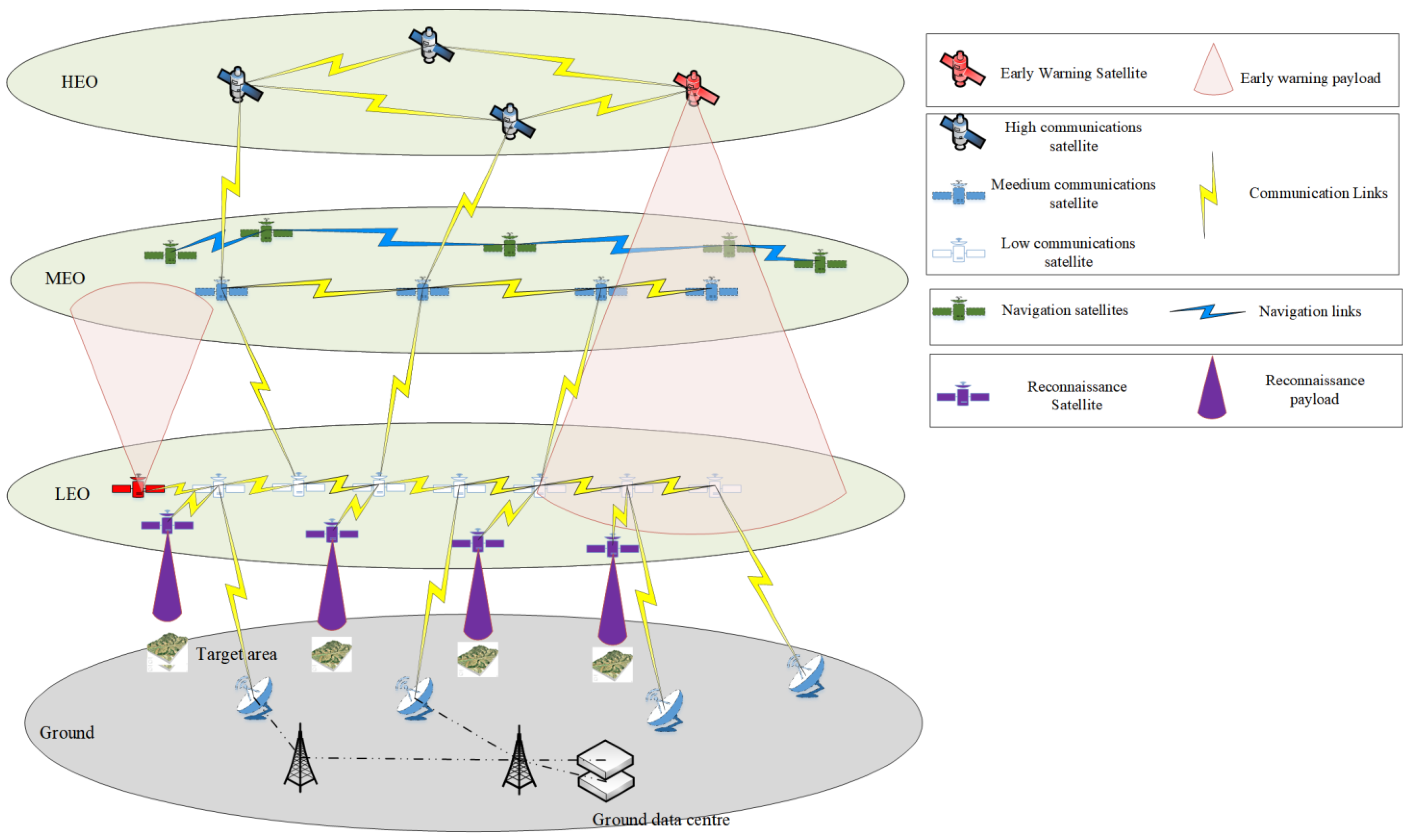
Figure 1. Structure of a space information network.
Aerospace 12 00841 g001
Figure 2. Global launch statistics (2014–2024).
Aerospace 12 00841 g002
Figure 3. (a) The actual distance is greater than the communication threshold; (b) the actual distance is less than the communication threshold; (c) the satellites are not visible to each other.
Aerospace 12 00841 g003
Figure 4. Analysis of data imbalance.
Aerospace 12 00841 g004
Figure 5. Workflow of proposed inter-satellite link prediction model.
Aerospace 12 00841 g005
Figure 6. Process of parameter optimization.
Aerospace 12 00841 g006
Figure 7. Comparison of loss function changes.
Aerospace 12 00841 g007
Figure 8. Threshold analysis for classification.
Aerospace 12 00841 g008
Figure 9. Validation of prediction effect.
Aerospace 12 00841 g009
Figure 10. Parametric analysis((ad): the number of hidden layers, (eh) the number of neurons in each layer, (il) the learning rate).
Aerospace 12 00841 g010
Figure 11. Analysis of dataset imbalance (antenna-pointing parameter).
Aerospace 12 00841 g011
Figure 12. Optimization curves for datasets A and B.
Aerospace 12 00841 g012
Figure 13. Analysis of data imbalance (communication distance).
Aerospace 12 00841 g013
Figure 14. Optimization process.
Aerospace 12 00841 g014
Table 1. Values of satellite parameters.
Parameter φ i ω Ω
Min.0000
Max.360180360360
Table 2. Parameters of real satellites.
Type of OrbitPair IDa/km e M/°i/° ω Ω
MEOOMNI-M111,637.8034.2444.99329.51325.78
O3B FM411,637.8032.13147.43353.906.14
O3B MPOWER F711,637.80178.7686.49138.61181.34
LEOCALSPHERE 17378.10120.8090.2163.38324.75
CALSPHERE 27378.101170.3490.2367.23202.11
DIGUI-327378.1091.530.028.93259.53
Table 3. Input dataset.
Pair ID φ i/° ω Ω φ i/° ω Ω
SO1–ST1180.001139.88233.55249.01290.3490.26324.80190.70
SO2–ST2357.71103.115.95225.84274.60155.73346.31274.15
SOi–STi318.39154.96196.14283.9655.1067.3592.99341.59
Table 4. Normalized input dataset.
Pair ID φ i/° ω Ω φ i/° ω Ω
SO1–ST10.500.770.640.690.800.500.900.52
SO2–ST20.990.570.010.620.760.860.960.76
SOi–STi0.880.860.540.780.150.370.250.94
Table 5. Output dataset.
Pair ID01234567287
SO1–ST1000000000
SO2–ST2010000000
SOi–STi000111100
Table 6. Optimization parameters and their ranges.
HyperparameterMeaningDefaultOptimization Range
mNumber of hidden layers2(2, 6)
nNumber of neurons in each layer32(32, 256)
eLearning rate 1 × 10 5 ( 1 × 10 5 , 1 × 10 2 )
ACoefficient a in the weighted loss function0.1(0.1, 5)
Table 7. Definition of the confusion matrix.
All CategoriesTrue Value
TrueFalse
Predicted valueTrueTPFP
FalseFNTN
Table 8. Results of parameter optimization.
A_ValueHidden_LayersLearning_RateNeurons_per_Layer
2.44325704960.001749911223
Table 9. Performance comparison.
AlgorithmAverage F1 ScoreAverage RecallAverage PrecisionTime
BO-FCNN0.910.930.892235.21
FCNN0.250.310.29896.08
BP0.440.610.34101.23
Random Forest0.050.020.25774.35
LSTM0.050.030.214716.01
Table 10. Optimal thresholds.
MetricValue
Average F1 Score0.91
Average Recall0.93
Average Precision0.89
Optimal Threshold0.80
Table 11. Performance metrics of the BO-FCNN model (case study).
MetricValue
Average F1 Score0.87
Average Recall0.90
Average Precision0.84
Optimal Threshold0.80
Table 12. Design of experiment.
Experimental Group IDModel StructureCore Verification ObjectivesKey Configurations
F0FCNNPerformance bottlenecks in validating empirical hyperparametersThree-layer full connection (128→128→128)
F1FCNN + Random Search (RS-FCNN)To verify the strengths of random search vs. empirical settings30-round random sampling hyperparameters (same search space as BO)
F2FCNN + Grid Search (GS-FCNN)To verify the difference in the efficiency and performance of grid search vs. random search30-round fixed-step grid sampling (same search space as BO)
F3FCNN + Bayesian Optimization (BO-FCNN)To verify the hyperparametric optimization advantage of Bayesian optimizationSurrogate model = GP-RBF; collection function = EI; 30 rounds of optimization (initial five random samples)
F4BO-FCNN-LSTMTo explore BO’s suitability in the temporal dimension (time series modeling + hyperparameter optimization synergy)Bo optimizes LSTM hyperparameters
F5LSTMTo verify the advantages of the BO-FCNN in the temporal dimension
Table 13. Comparison of model indicators.
Experimental Group IDModel StructureAverage F1 ScoreAverage RecallAverage PrecisionTimeCombination of Parameters
F0FCNN0.530.530.540{3-128-1}
F1RS-FCNN0.790.940.681399.43{5-128-4.46}
F2GS-FCNN0.730.940.597968{5-256-5}
F3BO-FCNN0.870.930.892935.21{5-249-4.76}
F4BO-FCNN-LSTM0.660.900.526313.94{2-82-4.98}
F5LSTM0.050.030.214716.01
Table 14. Stability analysis.
ModelAverage F1 ScoreCV (Average F1 Score)RMSECV(RMSE)
BO-FCNN0.8652 + 0.011513%0.1451 + 0.00755.7%
Table 15. Performance metrics and optimization parameters(antenna-pointing parameter).
DatasetAvg. F1 ScoremneA
Dataset A0.9860.0032531.43
Dataset B0.9160.0031464.25
Table 16. Performance metrics and optimization parameters (communication distance).
Communication DistancemNEaOptimal ThresholdAvg. F1 ScoreAvg. RecallAvg. Precision
11,00062460.00384.250.810.9180.930.90
10,50052450.00224.270.820.9320.940.91
10,00061970.00244.690.820.890.910.87
975042010.00244.600.810.820.870.78
950021390.00354.710.550.4130.590.32
92503460.00354.850.300.040.020.09
900032320.00921.570.3000.070.07
Disclaimer/Publisher’s Note: The statements, opinions and data contained in all publications are solely those of the individual author(s) and contributor(s) and not of MDPI and/or the editor(s). MDPI and/or the editor(s) disclaim responsibility for any injury to people or property resulting from any ideas, methods, instructions or products referred to in the content.