Reinforced Model Predictive Guidance and Control for Spacecraft Proximity Operations

Abstract

An increased level of autonomy is attractive above all in the framework of proximity operations, and researchers are focusing more and more on artificial intelligence techniques to improve spacecraft’s capabilities in these scenarios. This work presents an autonomous AI-based guidance algorithm to plan the path of a chaser spacecraft for the map reconstruction of an artificial uncooperative target, coupled with Model Predictive Control for the tracking of the generated trajectory. Deep reinforcement learning is particularly interesting for enabling spacecraft’s autonomous guidance, since this problem can be formulated as a Partially Observable Markov Decision Process and because it leverages domain randomization well to cope with model uncertainty, thanks to the neural networks’ generalizing capabilities. The main drawback of this method is that it is difficult to verify its optimality mathematically and the constraints can be added only as part of the reward function, so it is not guaranteed that the solution satisfies them. To this end a convex Model Predictive Control formulation is employed to track the DRL-based trajectory, while simultaneously enforcing compliance with the constraints. Two neural network architectures are proposed and compared: a recurrent one and the more recent transformer. The trained reinforcement learning agent is then tested in an end-to-end AI-based pipeline with image generation in the loop, and the results are presented. The computational effort of the entire guidance and control strategy is also verified on a Raspberry Pi board. This work represents a viable solution to apply artificial intelligence methods for spacecraft’s autonomous motion, still retaining a higher level of explainability and safety than that given by more classical guidance and control approaches.

1. Introduction

In recent years, space research has increasingly been shifting towards the enhancement of on-board spacecraft autonomy for all kind of missions, such as on-orbit servicing activities. In-orbit service and proximity operations may include a broad range of different activities, among which is the autonomous guidance and control of a chaser spacecraft around an uncooperative and unknown space object. The work presented here develops an innovative adaptive guidance algorithm for the path planning of the chaser’s trajectory around an uncooperative artificial object, aiming at reconstructing the shape and map of the object via imaging. In this context, the spacecraft autonomously explores the surrounding environment and plans the following actions to take. Thus, the problem falls in the Simultaneous Localization and Mapping (SLAM) framework, and since the planning operations are also performed, it is called active. SLAM may be phrased as a Partially Observable Markov Decision Process (POMDP), which entails an agent interacting with the environment and exchanging information with it. The goal is to solve the agent’s decision-making policy. To this end, deep reinforcement learning (DRL) techniques are employed, augmented with Model Predictive Control (MPC) to constrain the optimized trajectory for collision avoidance purposes.

1.1. Background and Motivation

Reinforcement learning (RL) algorithms are becoming a powerful tool when dealing with decision-making problems, and the combination with neural networks in DRL allows for improving the generalizing capabilities of the resulting policy, as they leverage domain randomization well to cope with model uncertainty. Several works have already underlined some of the beneficial effects of machine learning tools on spacecraft guidance and control enhancement, as treated in [1,2], and applications of deep reinforcement learning have already been analyzed in different scenarios and environments. Multiple contributions have been studied in [3,4,5] by Gaudet, Linares and Furfaro, where both planetary landing and close proximity operations were investigated. This work builds upon previous research on the topic in [6,7,8], where DRL for relative guidance is extensively tested. The main drawbacks of AI-based methods for performing these tasks are the complexity in validating the results and providing a mathematical proof for the optimal solution. Some recent works deal with the stability of dynamical systems controlled via neural networks [9,10], but more research is to be performed. When dealing with constrained optimization problems, the regions of the solution space that the agent cannot explore are only defined as part of the objective function, and, as such, it is not guaranteed that optimal decision-making always respects them. For an autonomous system, this is quite a problem, so in this work, the proposed methodology tries to overcome this issue by combining the generalizing capabilities and adaptivity of reinforcement learning with the capability to enforce constraints in the optimization of MPC. This approach has already been studied for a drone racing task in [11] but is still rather unexplored in the space GNC field. This combination results in an algorithm that maintains the advantages of learning-based methods by optimizing a non-differentiable task-level objective, as well as allowing the optimization of a cumbersome objective function such as the map reconstruction one, while simultaneously enforcing compliance with the constraints when tracking the DRL-generated trajectory with MPC, which offers precise actuation and ease in constraint handling, as treated for trajectory optimization in [12].

1.2. Points of Innovation

Considering the aforementioned approaches, the main innovative aspect of this work is the combination of the advantages of both RL and MPC. Specifically, the uncooperative target mapping scenario is intended to illustrate a case in which the objective function may be complex or even difficult to design. In such cases, resorting to the higher-level optimization provided by the reinforcement learning agent can be highly beneficial, enabling MPC to solve a much simpler problem in a fast and efficient manner. Measures of this kind are essential for ensuring the safe use of AI in space. The proposed solution is tested to verify its performance on an end-to-end AI-based simulator with image generation in the loop, tuned for proximity operations with an uncooperative target. This DRL formulation has also evolved with the innovative transformer neural network architecture, which is now one of the most intriguing and promising models [13]. Moreover, one of the most challenging activities to validate the potential applicability of this reinforcement learning-based methodology is guaranteeing optimal processor-in-the-loop (PIL) performances, compatible with the lower processing power commonly available in space. To achieve this, a PIL evaluation campaign on Raspberry Pi 4 has been exploited to validate the methodology. In summary, the key innovative contributions of this work are as follows:

• The coupling of DRL and MPC for uncooperative target mapping in a relative dynamics scenario;
• A PIL evaluation campaign to validate the methodology’s performance;
• The introduction of a transformer neural network architecture into the scenario already addressed in [6,7,8].

The following manuscript, at first, introduces the problem in Section 2; afterwards, the training and testing campaigns are presented in Section 3 and Section 4. Finally, the PIL validation analysis is treated in Section 5.

2. Problem Statement

This work proposes an innovative decision-making process to plan the pseudo-optimal guidance around an uncooperative space object autonomously, that is, the TANGO spacecraft from the PRISMA mission for this case study, with deep reinforcement learning. This process is coupled with Model Predictive Control, which optimizes the trajectory to minimize the difference with the DRL one while enforcing both action and state constraints. MPC is a powerful framework that can in principle handle both planning and control, including robustness to uncertainties. However, in practice, solving the full trajectory optimization problem online with MPC when the objective function formulation is cumbersome like the example mapping scenario described (nonlinear, non-convex, and non-differentiable) can become very time-consuming. In this framework, the DRL policy serves as an efficient global planner, quickly generating optimal reference trajectories online, while the MPC tracker then operates on a smaller-scaled problem, focusing on real-time constraint enforcement and disturbance rejection. This hierarchical split allows us to combine the best of both worlds. The overall pipeline describing such an approach is reported in Figure 1.

The input fed into the DRL agent is derived by an image processing estimation and navigation block, which returns realistic errors and noise in the filtered state. The autonomous guidance agent then crafts the guidance policy to maximize the reward function, and it is propagated online for a specified timespan, equal to the prediction horizon of the Model Predictive Controller. The linearized eccentric model, proposed by Inalhan et al. [14], is selected as a result of a trade-off between dynamics accuracy and computational efficiency. The equations are reported in Equation (1), considering the Local Vertical Local Horizontal (LVLH) reference frame centered at the target object center of mass:

$$\left\{\begin{array}{c}\ddot{x}={\displaystyle \frac{2\mu }{r^3}}x+2\omega \dot{y}+{\omega }^{2}x+a_x\hfill \\ \ddot{y}={\displaystyle \frac{-\mu }{r^3}}y-2\omega \dot{x}-{\omega }^{2}y+a_y\hfill \\ \ddot{z}={\displaystyle \frac{-\mu z}{r^3}}+a_z\hfill \end{array}\right.$$

(1)

where r is the radius of the target orbit, $\mu$ is the primary attractor gravitational parameter, and $\omega =\dot{f}$, defined in Equation (2), is the time derivative of the target true anomaly, expressed as follows:

$$\omega =\dot{f}={\displaystyle \frac{n{(1+ecosf)}^2}{{(1+e^2)}^{\frac{3}{2}}}}$$

(2)

with f being the target true anomaly, e its orbit eccentricity, and $n=\sqrt{{\displaystyle \frac{\mu }{r^3}}}$ the mean motion. Concerning the relative target attitude motion, the Euler equations for the target in the LVLH reference frame can be approximated as expressed in Equation (3).

$$\left\{\begin{array}{c}{I}_x{\ddot{\theta }}_x+n(I_z-I_y-I_x){\dot{\theta }}_y+n^2(I_z-I_x){\theta }_x=0\hfill \\ I_y{\ddot{\theta }}_y+n(I_x+I_y-I_z){\dot{\theta }}_x+n^2(I_z-I_x){\theta }_y=0\hfill \\ I_z{\ddot{\theta }}_z=0\hfill \end{array}\right.$$

(3)

with $I_x,I_y,I_z$ being the target object principal components of inertia, ${\theta }_x$, ${\theta }_y$, ${\theta }_z$ being the Euler angles around the three directions of the LVLH reference frame, and $\dot{{\theta }_i}$, $\ddot{{\theta }_i}$ being the corresponding first and second time derivatives.

The target object’s attitude motion is assumed to be completely random, while the chaser’s attitude is considered always fixed with respect to the target’s center (i.e., aligned with the center of the LVLH reference frame). Please refer to [8] for the analysis of a case where the chaser’s attitude is actively controlled using a PID controller, decoupled from the trajectory optimization. The generated trajectory in this time frame is then passed to the MPC optimizer, which returns the control actions the spacecraft should perform to adhere to the guidance while respecting constraints. Even in the cases in which the trajectory generated by the DRL agent satisfies the constraints, this hierarchical structure is still beneficial: the DRL agent optimizes the trajectory for a certain time horizon, acting like it is solving a Finite Horizon Optimal Control Problem. To achieve this, it propagates the equations of motion with its own internal model of the dynamics, as in Equation (1). Thus, coupling it with a Model Predictive Controller to track the generated trajectory allows us to compensate for model uncertainties and external disturbances by closing the loop locally. The two main components are described in the next sections.

2.1. DRL Guidance

Reinforcement learning is a widely employed tool for solving Markov Decision Problems (MDPs), [15], and its combination with neural networks, pioneered by [16], for function approximation allows many complex problems characterized by high dimensionality and partial observability to be solved. A state-of-the-art deep reinforcement learning algorithm, Proximal Policy Optimization (PPO), developed in [17], solves the spacecraft decision-making policy. Three main characteristics emerge from the decision-making problem: the state, the agent policy, and the reward function.

State space

This is the set of information coming from the image processing and navigation algorithms. The state vector fed to the agent should be tailored in such a way that it contains only essential information for the decision-making process to build a policy capable of selecting the appropriate action in every condition the agent may find itself. The state space, defined in Equation (4), comprises $\mathit{x}$ and $\dot{\mathit{x}}$, which are the relative position and velocity between the spacecraft and the target object, and $\mathit{\alpha }$ and $\dot{\mathit{\alpha }}$, which are the relative angular position and velocity.

$$\mathcal{S}=\left[\begin{array}{c}\mathit{x},\dot{\mathit{x}},\mathit{\alpha },\dot{\mathit{\alpha }}\end{array}\right]$$

(4)

Action space

The agent interacts with the surrounding environment, receiving the state observations and a reward signal and selecting the action to take accordingly. The action space modeled here assumes that the spacecraft can thrust in each of the six reference Cartesian frame directions, namely $x,-x,y,-y,z,-z$. The option of null action is also available to the agent. The thrust action then directly impacts the dynamics equation (computing the corresponding acceleration) in Equation (1). This formulation renders a direct and continuous control of the trajectory, consistent with an active SLAM problem. The action space is defined in Equation (5).

$$\mathcal{A}=\left[\begin{array}{c}{T}_{x_{+}},T_{x_{-}},T_{y_{+}},T_{y_{-}},T_{z_{+}},T_{z_{-}},0\end{array}\right]$$

(5)

This kind of control action is generated by a discrete action space, which means an action space with a constrained number of possible options. To consider a more realistic control action, a continuous action space may be identified; for a complete overview of this comparison, please refer to the analyses studied in Ref. [7].

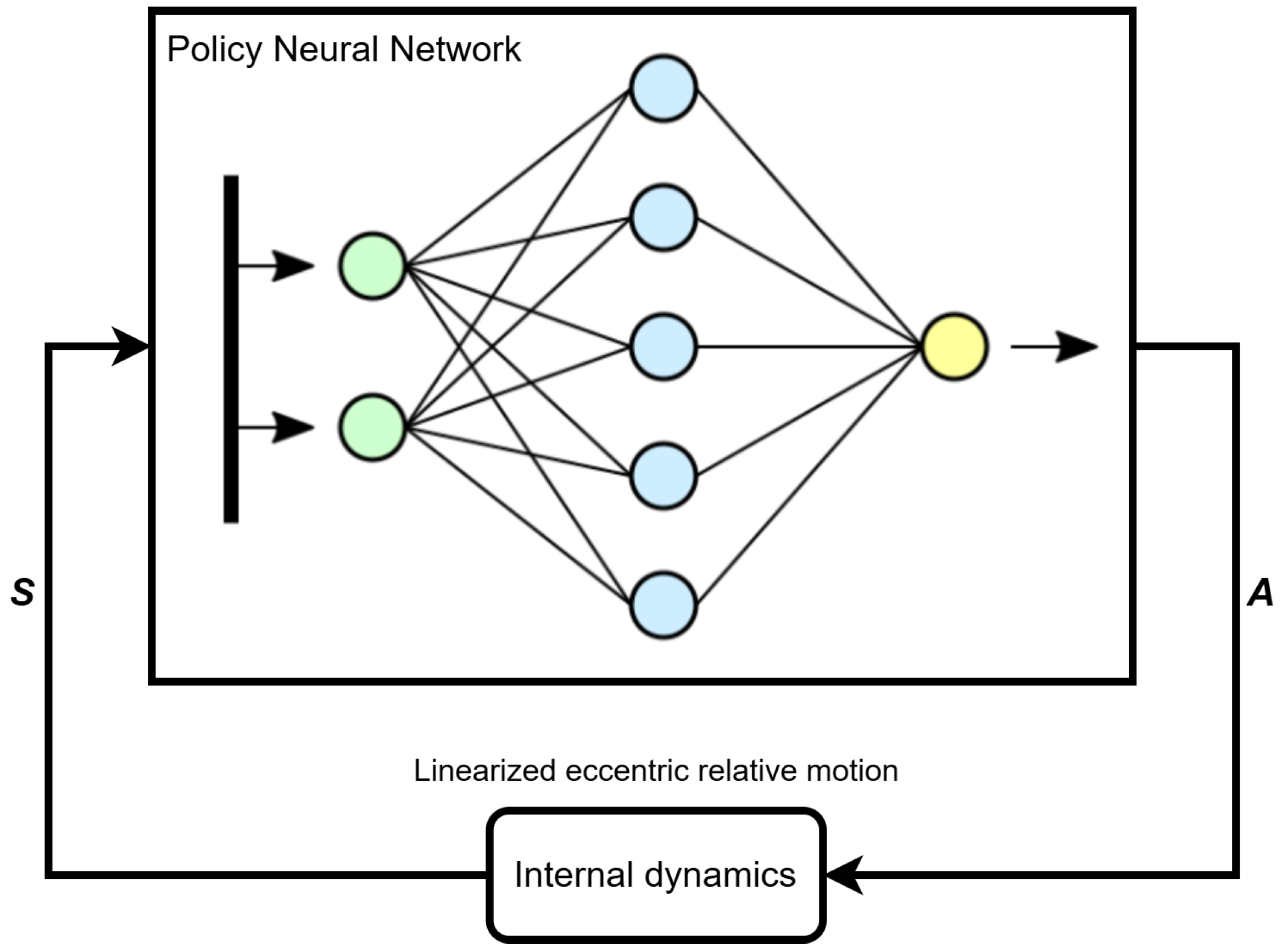
A block scheme of the state–action interaction is shown in Figure 2.

The state vector $\mathcal{S}$ and the action vector $\mathcal{A}$ are the ones defined in Equations (4) and (5). The selected internal dynamical model that is propagated is the one proposed in Ref. [14].

Reward function

The reward model always represents the most significant, critical, and delicate part of a DRL architecture, since the cumulative reward maximization drives the learning agent’s behavior. In the context of this work, the goal is to achieve a high-quality map of the target object together with a fast and safe process. The reward signals received by the agent are presented:

• Map level score. The faces that have both optimal Sun and camera exposure are the ones that generate an improvement in the level of the map. The maximum level defined for the map consists of having each face photographed $N_{accuracy}$ times. Therefore, at each time step the map level, $M{l}_{\%}$, can be computed considering how many good photos of each face have been taken until that moment. The corresponding reward score is defined in Equation (6), and at each time step k the agent is rewarded for increasing the map level over the current value, $M{l}_{\%,k-1}$.

  $$R_m=\left\{\begin{array}{cc}1\hfill & \mathrm{i}\mathrm{f}M{l}_{\%,k}>M{l}_{\%,k-1}\hfill \\ 0\hfill & \mathrm{o}\mathrm{t}\mathrm{h}\mathrm{e}\mathrm{r}\mathrm{w}\mathrm{i}\mathrm{s}\mathrm{e}\hfill \end{array}\right.$$

  (6)
  The improvement in the map depends on two different incidence angles between the target object faces and the Sun and camera directions:

  -

  Sun incidence score. The Sun incidence angle $\eta$ is the angle between the Sun direction relative to the target object and the normal to the face considered. The Sun incidence angle should be between 0° and 70° to avoid shadows or excessive brightness. Values outside this interval may correspond to conditions that degrade the quality of the image. If the angle exceeds this range, the photo can not be considered good enough to make a real improvement in the map.

  -

  Camera incidence score. The camera incidence angle $\epsilon$ is defined as the angle between the normal to the face and the camera direction. This angle should be maintained between 5° and 60°. Also in this case, if the angle exceeds this range, the photo can not be considered good enough to make a real improvement in the map.

• Position score. Negative scores are given when the spacecraft escapes from the region defined by a minimum and maximum distance from the target object, $D_{min}$ and $D_{max}$.

  $$R_d=\left\{\begin{array}{cc}-100\hfill & \mathrm{i}\mathrm{f}d\le D_{min}\mathrm{o}\mathrm{r}d\ge D_{max}\hfill \\ 0\hfill & \mathrm{o}\mathrm{t}\mathrm{h}\mathrm{e}\mathrm{r}\mathrm{w}\mathrm{i}\mathrm{s}\mathrm{e}\hfill \end{array}\right.$$

  (7)

2.2. MPC Optimization

Model Predictive Control (MPC) combines the benefits of optimal and feedback control methods. Initially, it leverages system dynamics knowledge to solve an optimal control problem (OCP) within a defined prediction horizon, discretized based on a chosen sampling step. Subsequently, optimized control is implemented for a set number of time steps determined by the control horizon. MPC aims to find the best control action by solving an optimization problem at each time step, considering future predictions and constraints. While it can provide excellent performance and stability for many systems, several factors can affect its ability to guarantee optimal behavior, like model accuracy as well as too restrictive constraints or a system operating near them. After the control step on the dynamics block, the sequence in Figure 1 is initiated once again, with the DRL agent providing the reference trajectory and the Model Predictive Control trying to optimize the control action to track it. One of the main advantages of using MPC is the straightforward implementation of constraints in the computation of the control action. Apart from the usual constraint on maximum spacecraft thrust, this work focuses on the implementation, in a convex form, of collision avoidance, as it cannot be guaranteed by the DRL guidance. The primary limitation of Model Predictive Control lies in the computational time required to solve the optimal control problem at each time step, prompting the initial use of an analytic model. Moreover, convexifying the optimization cost function and constraints enables leveraging convex optimization solvers, thereby achieving a swift and effective solution suitable for autonomous control, as in [18,19]. The objective of MPC is to find the control acceleration that minimizes a weighted function of tracking error with respect to the trajectory generated by the DRL agent and fuel cost. This can be effectively treated as an optimal control problem and a brief mathematical description is now presented. The problem can be expressed as in Equation (8):

$$\begin{array}{cc}\hfill \mathrm{minimize}\hfill & J\left(\mathbf{Z}\right(t\left)\right)\hfill \\ \hfill \mathrm{subject}\mathrm{to}\hfill & \dot{\mathbf{x}}\left(t\right)=f\left(\mathbf{x}\left(t\right)\right)+\mathbf{B}\mathbf{u}\left(t\right),\hfill \\ \hfill & {\parallel \mathbf{u}\left(t\right)\parallel }_p\le T_{\max },\hfill \\ \hfill & \parallel \mathbf{C}(\mathbf{x}\left(t\right)-{\mathbf{x}}_c\left(t\right)){\parallel }_2\ge R_{\mathrm{col}},\hfill \end{array}$$

(8)

where $\mathbf{Z}$ is the decisional vector, which contains both the state x (relative position and velocity) and the control action u. $f\left(\mathbf{x}\right(t\left)\right)$ refers to a generic model for description of the satellite relative dynamics, $T_{max}$ is the maximum specific thrust, $R_{col}$ specifies the minimum allowable distance between the two spacecrafts, and ${\mathbf{x}}_c\left(t\right))$ is the position vector of the client, which is zero assuming it is at the origin of the LVLH reference frame, while the matrices $\mathbf{B}$ and $\mathbf{C}$ are defined as in Equation (9).

$$\mathbf{B}=\left[\begin{array}{ccc}0& 0& 0\\ 0& 0& 0\\ 0& 0& 0\\ 1& 0& 0\\ 0& 1& 0\\ 0& 0& 1\end{array}\right],\mathbf{C}=\left[\begin{array}{cccccc}1& 0& 0& 0& 0& 0\\ 0& 1& 0& 0& 0& 0\\ 0& 0& 1& 0& 0& 0\end{array}\right].$$

(9)

The problem in Equation (8) is continuous and nonlinear. The resolution strategy chosen in this work follows the procedure in [20] to make the optimization convex. For the collision avoidance constraint, which is the main source of non-convexity, the solution adopted in [18] is used: this strategy involves generating separating planes between the satellites, converting the circular prohibited zone into a suitable convex formulation.

$${\left(\overline{\mathbf{x}}\left[k\right]-{\overline{\mathbf{x}}}_c\left[k\right]\right)}^T{\mathbf{C}}^T\mathbf{C}\left(\mathbf{x}\left[k\right]-{\mathbf{x}}_c\left[k\right]\right)\ge R_{col}{∥\mathbf{C}\left(\overline{\mathbf{x}}\left[k\right]-{\overline{\mathbf{x}}}_c\left[k\right]\right)∥}_2$$

(10)

$\overline{\mathbf{x}}$ provides an initial guess of the spacecraft’s optimal trajectory, while $\mathbf{C}$ is a matrix designed to extract only the position components from the solution. For a more in-depth explanation of all the mathematical steps, please refer to [18,19,20]. The main parameters defining the MPC implementation are reported in

Table 1. Model Predictive Control implementation parameters.

Parameter	Value
Prediction Horizon	400 s
Sampling Time $T_s$	10 s
Control Horizon	$10\ast T_s$
$u_{max}$	$0.01$ m/s
S	1000
R	10

.

S and R are the state error and control weight identity matrices, respectively, which affect the optimization solver, while $u_{max}$ is the maximum allowable value for the control action. The problem is solved with the cvx library ([21]) for convex optimizations, returning the control profile for the full prediction horizon, which also corresponds to the propagation time of the online reinforcement learning agent. From this profile, only the first 10 sample times are used, according to the specified control horizon.

3. Training Results

The deep reinforcement learning agent is first trained offline before deploying its decision-making policy in the entire GNC pipeline. Two different network definitions are employed to approximate the mapping function between the input state and the output actions:

• At first, a recurrent neural network architecture is selected because of its improved stability when dealing with evolving dynamics with respect to simple feed-forward networks, as already analyzed in [8]. Among the different types of RNNs, here the Long Short-Term Memory (LSTM) recurrent layer is exploited. The definition of the network is presented in

  Table 2. Policy network for recurrent architecture [8].

  Layer	Elements	Activation
  LSTM Layers	24	-
  1st Hidden Layer	64	ReLU
  2nd Hidden Layer	32	ReLU
  Learning rate	${10}^{-5}$	-

  .
• Secondly, a transformer network formulation, the state-of-the-art network for this complex problem, is investigated. The transformer architecture consists of self-attention mechanisms and feed-forward neural networks, as introduced in [13]. This kind of architecture was originally developed for natural language processing (NLP), excelling at capturing dependencies and relationships across sequences, making it suitable for tasks where understanding context and long-range dependencies is crucial. Overall, transformer architectures also offer a promising direction in deep reinforcement learning for continuous action spaces, especially when the problem involves learning complex dependencies and patterns. The architecture defined for the transformer agent is presented in

  Table 3. Policy network for transformer architecture.

  Layer	Elements
  Embedding Layer	128
  Encoder	128, head = 4, layers = 2
  Output Layer	128
  Learning rate	${10}^{-4}$

  .

The training process is performed with randomized initial conditions regarding all the variables affecting the input state of the policy. This is conducted to stress the generalization capabilities of the neural network architecture to obtain an agent that can consistently perform well, whatever the initial conditions of the state variables are. For this reason, at the start of each episodic simulation run, they are randomly generated inside a certain range, reported in

Table 4. State variables initial condition ranges.

Variable	Range
d	$2D_{min}<d<0.5D_{max}$
$\alpha$	$0^{\circ }<\alpha <{360}^{\circ }$
$\delta$	$-{90}^{\circ }<\delta <{90}^{\circ }$
v	0 m/s
${\theta }_i$	$0^{\circ }$
${\dot{\theta }}_i$	$-0.1$ rad/s $<{\dot{\theta }}_i<0.1$ rad/s

, where d and v are the relative position and velocity between the chaser and the target, $\alpha$ and $\delta$ represent the azimuth and the elevation angle, respectively, and finally $\theta$ and $\dot{\theta }$ express the rotation angles and velocity of the target, with $i\in$ [1:3] specifying the axis. $D_{min}=1.5$ m and $D_{max}=35$ m are the two boundaries defining the possible stopping condition of an episode.

Both the actor and the critic network models are periodically updated during the training phase with an epoch of 10 episodes, whose steps are divided into random batches of dimension 32. A single training episode terminates when the target object map is completely acquired or when the spacecraft’s trajectory overcomes the region defined by the minimum and maximum distance from the target or if a maximum time window is achieved. The hyperparameters of the DRL selected algorithm, that is, PPO for its proven capabilities and state-of-the-art performance in several benchmark scenarios, are summarized in

Table 5. PPO and training hyperparameters.

Variable	Value
Reward Discount Factor $\gamma$	0.99
Terminal Reward Discount Factor $\lambda$	0.95
Clipping Factor $ϵ$	0.2
Entropy Factor $s_2$	0.02
Optimizer	ADAM
Optimization Step Frequency	10 episodes
Training Episodes	18,000

.

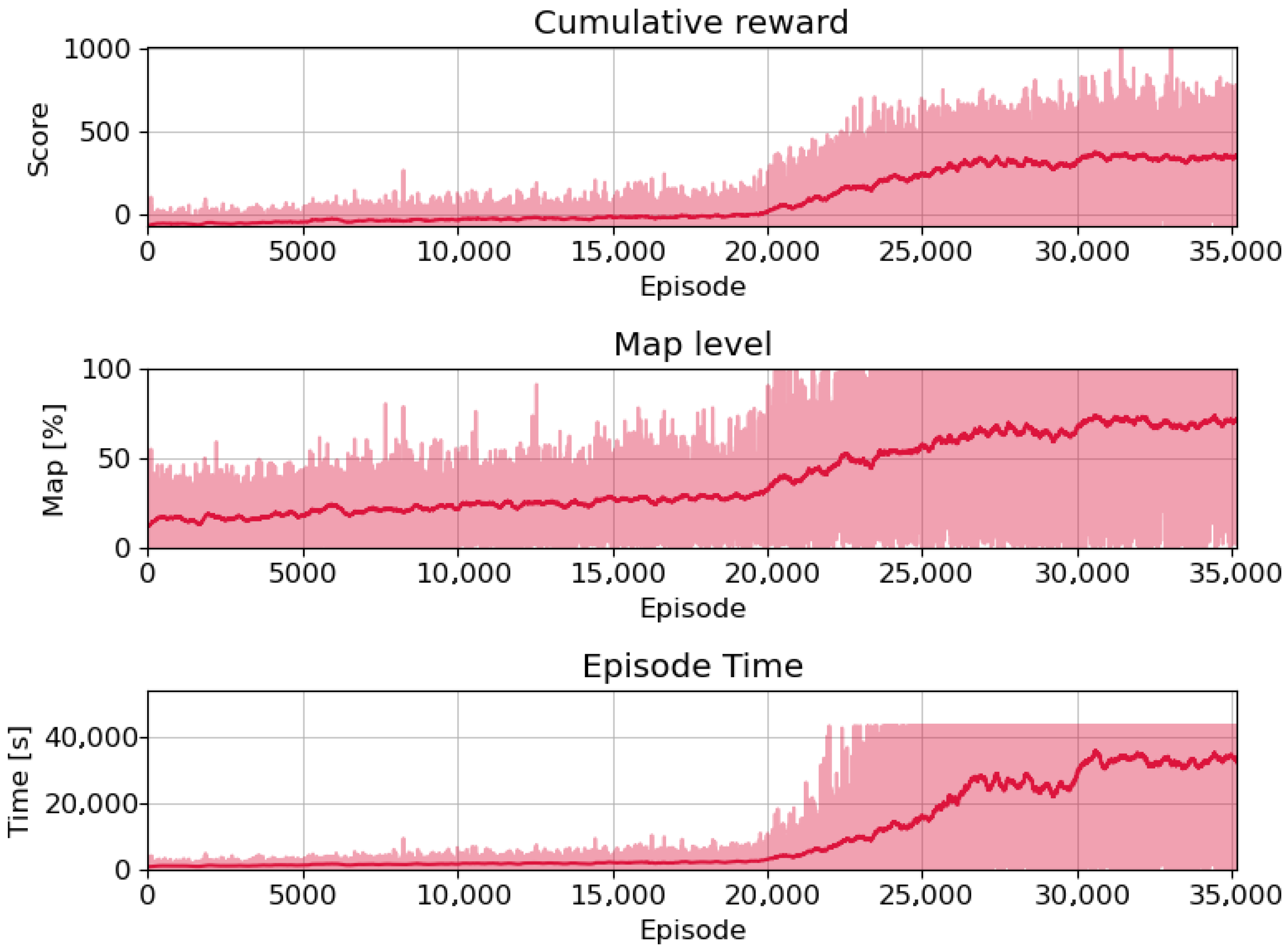
The training trend results, in terms of cumulative reward, map level percentage, and time, are reported in Figure 3 for the recurrent architecture and in Figure 4 for the transformer.

The profiles increase over time, meaning that the spacecraft adjusts its decision-making towards an improved map reconstruction, and it is able to remain inside the specified region of space for longer. The recurrent network achieved better performance in terms of metrics and training time, even if the transformer one presents more stability over time and therefore potentially robustness. Moreover, looking at the training trend, it seems that there is still room for improvement.

4. Testing Campaign

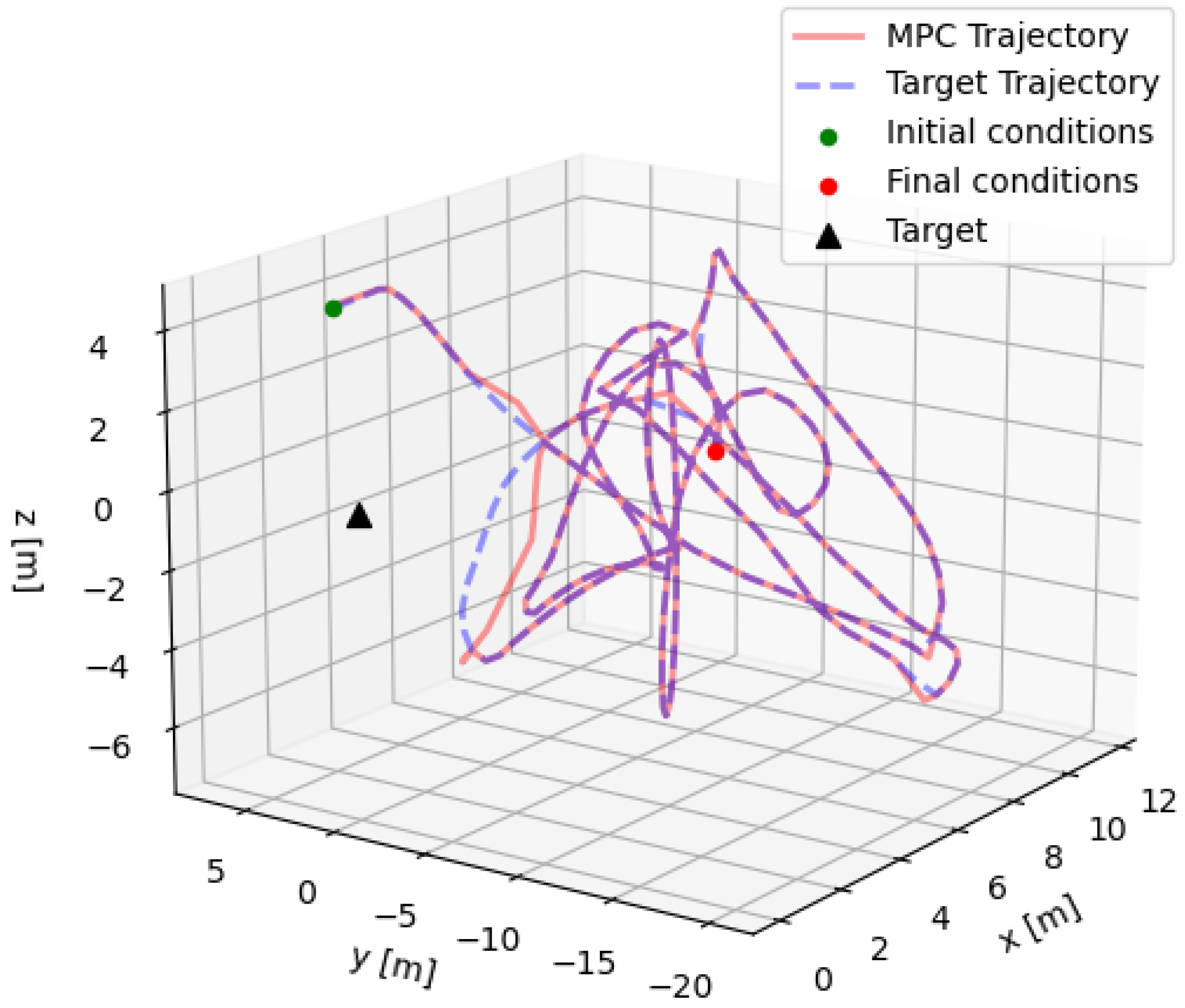
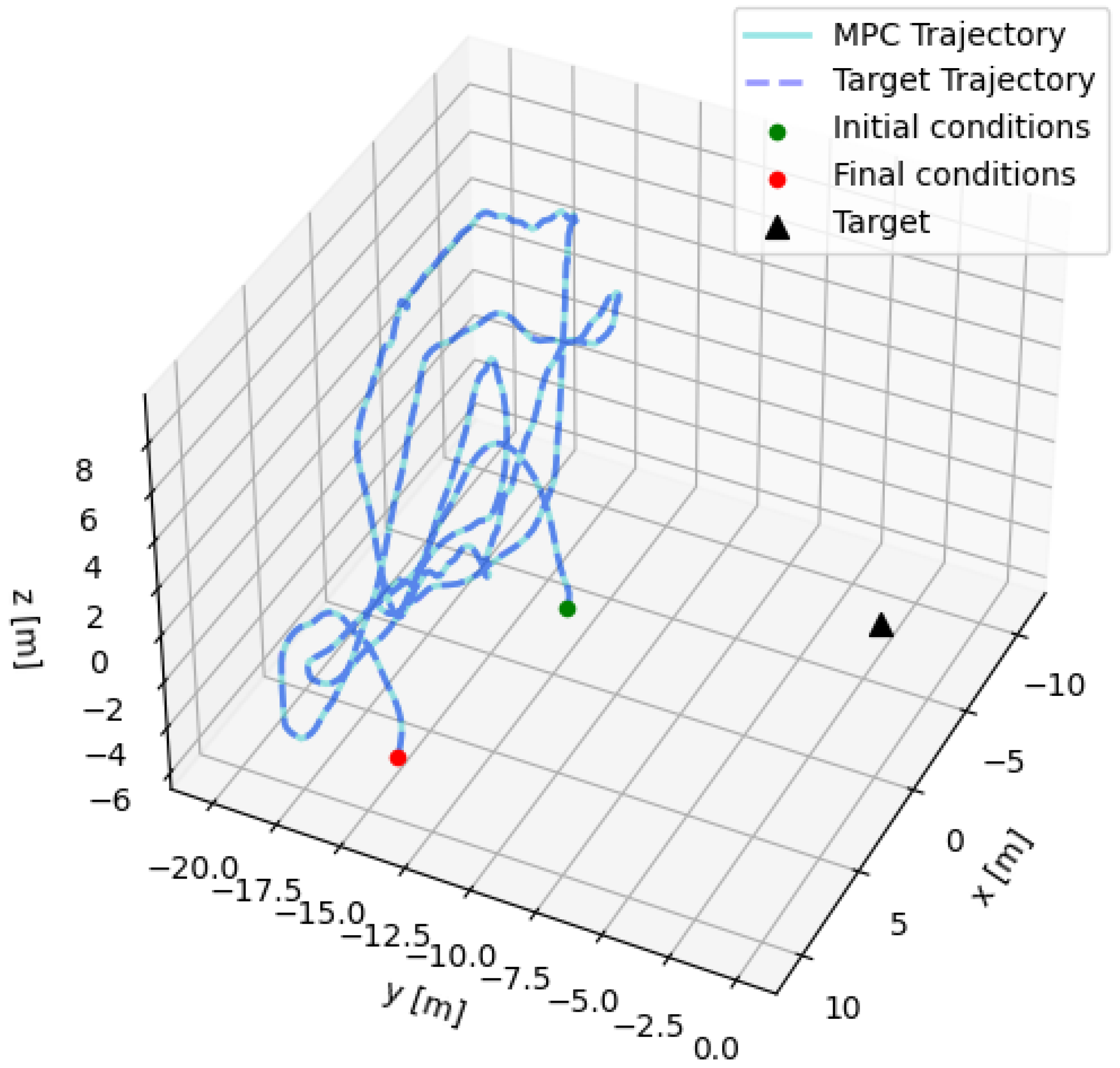
Once the training phase is concluded, the output policy network is tested to understand the effective performance in nominal conditions. The agent is inserted in the overall simulator architecture and coupled with the convex MPC formulation with the collision avoidance constraint. This constraint is set to 5 m, which is a higher value with respect to the one used to design the RL reward function, to verify the correctness of the complete guidance and control algorithm. Example trajectories from a random simulation for the two neural network architectures are reported in Figure 5 and Figure 6.

As is visible, the MPC correctly tracks the trajectory generated by the DRL agent, except when the latter comes too close to the target. When this happens, the optimization enforces the collision avoidance constraint, which then shapes the trajectory to remain outside of the boundary region, ensuring safe operations. This is particularly visible in Figure 5. Indeed, the transformer neural policy learns an interesting behavior, which is moving the chaser spacecraft to a particular relative position with respect to the target and maintaining it in that zone, taking advantage of the target tumbling to obtain pictures of all its faces. This strategy, though effective for the map reconstruction, is much slower than the one retrieved by the recurrent policy, and this point is confirmed when looking at the average episode time, which is a almost double in the transformer case, while the performance in terms of map percentage is quite comparable.

A new testing campaign is performed on the high-fidelity simulator to check the robustness of the algorithm against noise and uncertainty coming from the image processing and navigation blocks, providing the input state, and the mapping level with the trajectory imposed by the MPC following the DRL guidance. Different noise levels are tested, up to 12 dB for the image generation step, leading to a compounding error from image processing and navigation lower than $5\%$ in relative range and $5^{\circ }$ in mean angular error. The results are reported in

Table 6. Comparison of average map performance for different DRL network architectures.

	Recurrent	Transformer
Average Map	84.3%	79.1%

.

In this study, both the recurrent DRL architecture and the transformer-based architecture were evaluated. The recurrent approach exhibited higher performance, while the transformer variant demonstrated greater stability. At this level of task complexity, these differences do not lead to a definitive preference for one architecture over the other, as both satisfy the intended objectives of the proposed framework. A conclusive choice would require extending the analysis to more complex scenarios, which lies beyond the present scope but represents a promising direction for future work.

5. Processor-in-the-Loop Validation

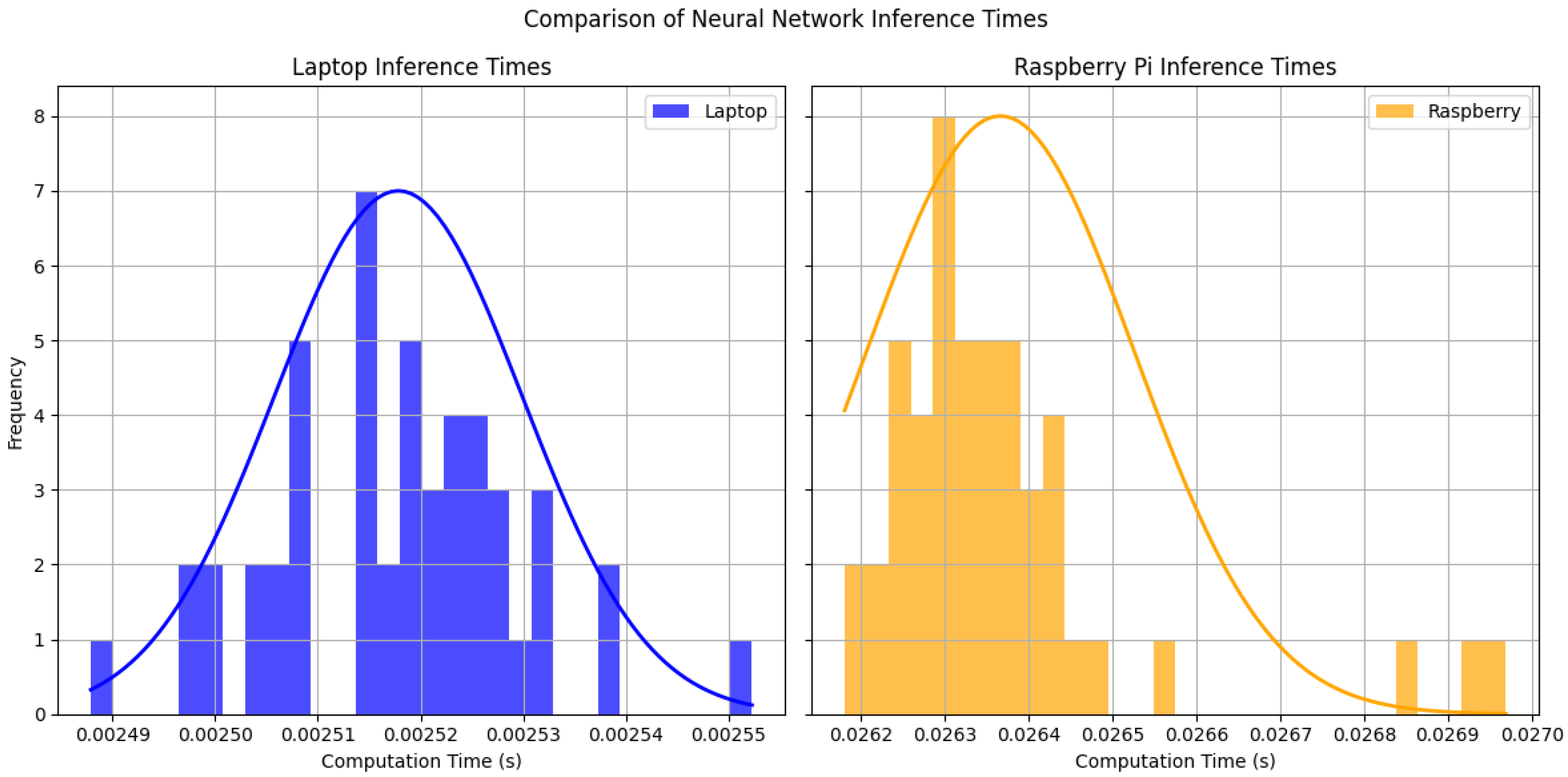
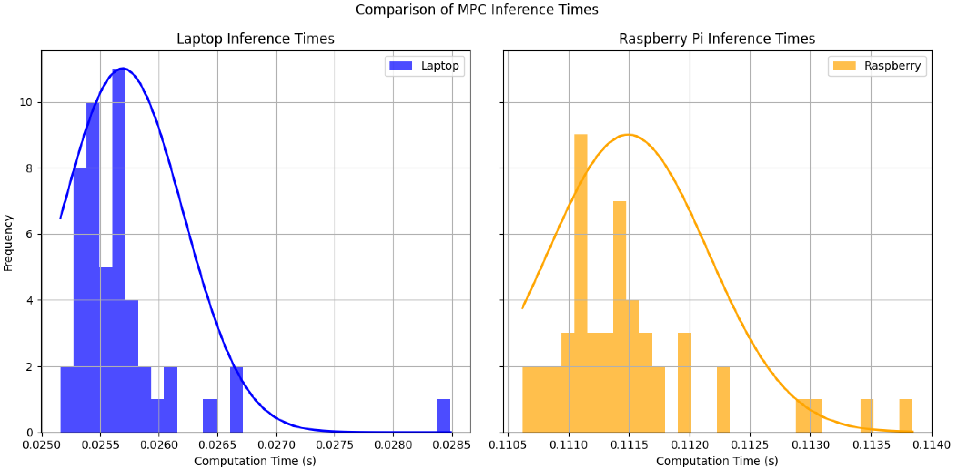
To verify the potential application of such an algorithm for online optimization, the whole guidance and control strategy is tested on a Raspberry Pi 4 (Raspberry Pi Foundation, Shenzhen, China), which should emulate the lower processing power available in space. It is equipped with a Broadcom BCM2711 quad-core Cortex-A72 (ARM v8) 64-bit SoC (Broadcom Inc., San Jose, CA, USA), operating at 1.8GHz. The Raspberry Pi has previously been used in space missions, including ESA’s Astro Pi mission, and has served as a testbed in various CubeSat systems. This makes it a compelling candidate for inclusion in this study. Running models on the Raspberry Pi 4 is straightforward due to its Linux-based operating system, Raspbian, which allows PyTorch 2.2.2 models to be loaded into a Python 3.10 script and executed directly. The procedure followed to deploy the guidance algorithm on this board is straightforward, since it natively supports Python. This allows the entire simulation framework to run directly on the device without the need to compile the code or adapt it to a different architecture, making the process quick and efficient. Here, the attention is focused primarily on the processing time required to run the guidance and control strategy to verify that it could be compatible with mission operations. The results with the recurrent neural network architecture are reported in Figure 7 and Figure 8, but similar outcomes can be expected with the transformer inference.

The Raspberry Pi 4 is about one order of magnitude slower, but still the entire guidance and control implementation takes less than $0.12$ seconds to run. The output is also validated and the error between the values coming from the two machines is negligible. Some information regarding the machines used is reported here for completeness:

• Laptop: Dell Precision 5680-Intel Core i9 13900H, 2.6 GHz (Intel, Santa Clara, CA, USA)
• Raspberry Pi 4: Quad-core Cortex-A72 (ARM v8) 64-bit SoC @ 1.8GHz

6. Conclusions

The proposed work deals with an adaptive guidance and control algorithm to autonomously reconstruct the geometry and shape of the selected uncooperative artificial object in space. The guidance block is implemented with a state-of-the-art deep reinforcement learning algorithm to design the decision-making policy of the spacecraft agent, which is approximated by two different network models: recurrent and transformer. RL can directly optimize a task-level objective and can leverage domain randomization to cope with model uncertainty, allowing the discovery of more robust control responses. This method’s primary limitation lies in the challenge of mathematically confirming its optimality and the inability to directly incorporate constraints outside the objective function, thus potentially leading to solutions that do not fully meet the constraints. To address this, a convex Model Predictive Control framework is utilized to follow the RL-derived trajectory while ensuring adherence to the constraints. The overall pipeline results in terms of average map reconstruction are consistent with the performance of the RL guidance, but this time collision avoidance with the target is ensured by MPC. The two different neural architectures are proposed and compared: a recurrent one employing LSTM layers and a transformer network, using self-attention mechanisms to capture dependencies in sequences of data points. The whole guidance and control platform is also tested on a Raspberry Pi board to verify the computational effort on less potent hardware. This validation proves the capabilities of the strategy and could be used as a reference when comparing the proposed guidance and control pipeline with more classical approaches, which would be an important step towards the verification of the advantages of this new methodology.

References

1. Izzo, D.; Märtens, M.; Pan, B. A survey on artificial intelligence trends in spacecraft guidance dynamics and control. Astrodynamics 2019, 3, 287–299. [Google Scholar] [CrossRef]
2. Silvestrini, S.; Lavagna, M. Deep Learning and Artificial Neural Networks for Spacecraft Dynamics, Navigation and Control. Drones 2022, 6, 270. [Google Scholar] [CrossRef]
3. Linares, R.; Campbell, T.; Furfaro, R.; Gaylor, D. A Deep Learning Approach for Optical Autonomous Planetary Relative Terrain Navigation. Spacefl. Mech. 2017, 160, 3293–3302. [Google Scholar]
4. Gaudet, B.; Linares, R.; Furfaro, R. Adaptive Guidance and Integrated Navigation with Reinforcement Meta-Learning. Acta Astronaut. 2020, 169, 180–190. [Google Scholar] [CrossRef]
5. Gaudet, B.; Linares, R.; Furfaro, R. Deep reinforcement learning for six degree-of-freedom planetary landing. Adv. Space Res. 2020, 65, 1723–1741. [Google Scholar] [CrossRef]
6. Brandonisio, A.; Lavagna, M.; Guzzetti, D. Reinforcement Learning for Uncooperative Space Objects Smart Imaging Path-Planning. J. Astronaut. Sci. 2021, 68, 1145–1169. [Google Scholar] [CrossRef]
7. Capra, L.; Brandonisio, A.; Lavagna, M. Network architecture and action space analysis for deep reinforcement learning towards spacecraft autonomous guidance. Adv. Space Res. 2022, 71, 3787–3802. [Google Scholar] [CrossRef]
8. Brandonisio, A.; Bechini, M.; Civardi, G.L.; Capra, L.; Lavagna, M. Closed-loop AI-aided image-based GNC for autonomous inspection of uncooperative space objects. Aerosp. Sci. Technol. 2024, 155, 109700. [Google Scholar] [CrossRef]
9. Izzo, D.; Tailor, D.; Vasileiou, T. On the Stability Analysis of Deep Neural Network Representations of an Optimal State Feedback. IEEE Trans. Aerosp. Electron. Syst. 2020, 57, 145–154. [Google Scholar] [CrossRef]
10. Korda, M. Stability and Performance Verification of Dynamical Systems Controlled by Neural Networks: Algorithms and Complexity. IEEE Control Syst. Lett. 2022, 6, 3265–3270. [Google Scholar] [CrossRef]
11. Romero, A.; Song, Y.; Scaramuzza, D. Actor-Critic Model Predictive Control. arXiv 2024, arXiv:2306.09852. [Google Scholar] [CrossRef]
12. Smith, T.K.; Akagi, J.; Droge, G. Model predictive control for formation flying based on D’Amico relative orbital elements. Astrodynamics 2025, 9, 143–163. [Google Scholar] [CrossRef]
13. Vaswani, A.; Shazeer, N.; Parmar, N.; Uszkoreit, J.; Jones, L.; Gomez, A.N.; Kaiser, L.; Polosukhin, I. Attention Is All You Need. arXiv 2023, arXiv:1706.03762. [Google Scholar] [PubMed]
14. Inalhan, G.; Tillerson, M.; How, J. Relative Dynamics and Control of Spacecraft Formations in Eccentric Orbits. J. Guid. Control. Dyn. 2002, 25, 48–59. [Google Scholar] [CrossRef]
15. Sutton, R.S.; Barto, A.G. Reinforcement Learning: An Introduction; The MIT Press: Cambridge, MA, USA, 2015. [Google Scholar]
16. Mnih, V.; Badia, A.P.; Mirza, M.; Graves, A.; Lillicrap, T.P.; Harley, T.; Silver, D.; Kavukcuoglu, K. Asynchronous Methods for Deep Reinforcement Learning. arXiv 2016, arXiv:1602.01783. [Google Scholar] [CrossRef]
17. Schulman, J.; Wolski, F.; Dhariwal, P.; Radford, A.; Klimov, O. Proximal Policy Optimization Algorithms. arXiv 2017, arXiv:1707.06347. [Google Scholar] [CrossRef]
18. Morgan, D.; Chung, S.J.; Hadaegh, F. Model Predictive Control of Swarms of Spacecraft Using Sequential Convex Programming. J. Guid. Control Dyn. 2014, 37, 1–16. [Google Scholar] [CrossRef]
19. Belloni, E.; Silvestrini, S.; Prinetto, J.; Lavagna, M. Relative and absolute on-board optimal formation acquisition and keeping for scientific activities in high-drag low-orbit environment. Adv. Space Res. 2023, 73, 5595–5613. [Google Scholar] [CrossRef]
20. Sarno, S.; Guo, J.; D’Errico, M.; Gill, E. A guidance approach to satellite formation reconfiguration based on convex optimization and genetic algorithms. Adv. Space Res. 2020, 65, 2003–2017. [Google Scholar] [CrossRef]
21. Agrawal, A.; Verschueren, R.; Diamond, S.; Boyd, S. A rewriting system for convex optimization problems. J. Control Decis. 2018, 5, 42–60. [Google Scholar] [CrossRef]
Figure 1. Reinforced model predictive guidance and control scheme.
Aerospace 12 00837 g001
Figure 2. Policy neural network decision-making.
Aerospace 12 00837 g002
Figure 3. TANGO case study training of the recurrent DRL agent: metric (reward score, map level, and episode time) evolution along the simulation [8].
Aerospace 12 00837 g003
Figure 4. TANGO case study training of the transformer DRL agent: metric (reward score, map level, and episode time) evolution along the simulation.
Aerospace 12 00837 g004
Figure 5. Example trajectory of recurrent DRL guidance + MPC.
Aerospace 12 00837 g005
Figure 6. Example trajectory of transformer DRL guidance + MPC.
Aerospace 12 00837 g006
Figure 7. Comparison between laptop and Raspberry Pi 4 recurrent neural network inference time.
Aerospace 12 00837 g007
Figure 8. Comparison between laptop and Raspberry Pi 4 Model Predictive Control optimization time.
Aerospace 12 00837 g008