Abstract
A high-performance diffuser is crucial for a high-pressure ratio centrifugal compressor to achieve high efficiency. Pipe diffusers have been proven effective in enhancing the performance of such compressors. However, detailed design methodologies for pipe diffusers are scarcely covered in the existing literature. Thus, this paper provides a comprehensive design methodology specifically for fishtailed pipe diffusers. This methodology begins by defining the throat and outlet areas using gas-dynamic functions and then establishes the centerline by choosing the angle distributions. Finally, various cross-sectional profiles are defined along the centerline, completing the diffuser’s design. To demonstrate the proposed methodology, a fishtailed pipe diffuser is designed to contrast with the original diffuser of the National Aeronautics and Space Administration’s High-Efficiency Centrifugal Compressor (NASA HECC). Numerical analysis shows that the fishtailed pipe diffuser increases the compressor’s total pressure ratio and isentropic efficiency over its whole operating range. At the design operating point, the isentropic efficiency and the total pressure ratio are increased by 2.4 percentage points and 2.7%, respectively. This demonstrates the effectiveness of the proposed design methodology for fishtailed pipe diffusers.
1. Introduction
Centrifugal compressors find extensive application in gas turbines and small aero engines owing to their ability to achieve higher single-stage total pressure ratios, and enable more compact designs compared to axial compressors. However, their efficiency is often compromised by complex secondary flow phenomena, particularly within the diffuser section. This issue becomes significantly challenging in high-pressure ratio centrifugal compressors, where supersonic inlet flows in the diffuser induce substantial shock losses and downstream flow degradation. Hence, there is a critical need for researchers to comprehensively understand the flow mechanisms within the diffuser system and to develop high-performance diffuser designs.
The pipe diffuser, pioneered by Vrana [1] and Kenny [2], has emerged as a preferred solution for high-pressure ratio centrifugal compressors. This design effectively mitigates the adverse effects of high inlet Mach numbers, accommodates highly distorted inlet flows, and offers cost-effective manufacturing solutions. Manufacturers such as General Electric [3] and Pratt & Whitney [4] have embraced this type of diffuser due to its demonstrated ability to deliver superior performance under demanding operational conditions. As shown in Figure 1, pipe diffusers are generally categorized into two types: the radial pipe diffuser and the fishtailed pipe diffuser. Both of these diffusers share a common section, namely the radial–conical section, as illustrated in Figure 1b. This section shows some similarities with traditional radial vaned diffusers, such as channel and wedge diffusers. It consists of a vaneless space and semi-vaneless space located ahead of the throat. Apart from these parts, the pipe diffuser distinguishes itself with a unique region between the vaneless space and the semi-vaneless space, known as the pseudo-vaneless space. This region is formed by the intersection of two adjacent pipe passages and features a distinctive sharp leading edge, referred to as the scalloped leading edge [5]. The planar projection and geometry configuration of the scalloped leading edge are illustrated in Figure 1a,b, respectively. Additionally, the throat of the pipe diffuser is characterized by a cylindrical-like region, implying the throat area remains constant. In the radial pipe diffuser, the radial–conical section is directly followed by a straight pipe with constant cross-sectional area, allowing the airflow to remain in the radial direction. Downstream components, such as a bend and an axial diffuser, are then introduced to redirect the flow from radial to axial [6,7]. For the fishtailed pipe diffuser, an additional bend is integrated to the end of the radial–conical section, enabling the airflow to transition directly from a radial to an axial direction [7,8].
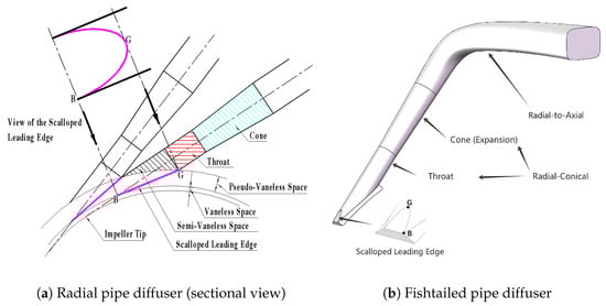
Figure 1.
Schematic diagram of two pipe diffusers.
Over the past two decades, various design methodologies have been explored for pipe diffusers, encompassing both radial pipe diffusers and fishtailed pipe diffusers. Bennett [9] and Antas [10] each proposed methodologies for designing radial pipe diffusers. Bennett’s methodology primarily emphasizes conceptual design principles, whereas Antas provides a more comprehensive and detailed derivation of the relevant formulas. Fishtailed pipe diffusers involve significantly more intricate design methodologies, as they have the capability to redirect airflow from a radial to an axial direction along a complex centerline with specified cross-sectional profiles. The design concept for fishtailed pipe diffusers introduced by Wang [11] represents the earliest documented methodology. Subsequently, Antas [12] and Xie [13] developed more detailed design methodologies for fishtailed pipe diffusers.
Nonetheless, most existing documents focus primarily on basic design concepts, and there is a lack of detailed formulas and theoretical guidance for the design of fishtailed pipe diffusers. Additionally, existing studies all fall short in exploring the specific conditions required for the formation of scalloped leading edges, leading to the possibility that some diffuser designs may not include this feature. To fill the gap, this paper introduces a comprehensive design methodology for a fishtailed pipe diffuser, and outlines the critical conditions for forming scalloped leading edges. A practical application of the proposed methodology is presented to demonstrate its effectiveness.
The structure of this paper is organized as follows: Section 2 delves into the comprehensive methodology for designing a fishtailed pipe diffuser. Section 3 elaborates on the specific design details of a fishtailed pipe diffuser for the National Aeronautics and Space Administration’s High-Efficiency Centrifugal Compressor (NASA HECC) [14]. Section 4 illustrates the details of the numerical setting-up, including the solver configuration, grid generation and independence study, boundary conditions, and an investigation into the selection of turbulence models. Section 5 conducts a comparative analysis of the performance characteristics of the prototype design (the NASA HECC compressor) and the prototype impeller with a fishtailed pipe diffuser. Finally, Section 6 and Section 7 present a conclusion and discussion, respectively.
2. Design Methodology
The design process begins with determining the throat and outlet areas based on aerodynamic parameters. The centerline of the fishtailed pipe diffuser is then defined, comprising two segments: the radial–conical section and the radial-to-axial section. Subsequently, the cross-sections along the centerline are designed in accordance with the specified area distribution. The design is finalized by defining the scalloped leading edge and the vaneless space [15].
2.1. Throat and Outlet Areas
To determine the throat and outlet areas of the fishtailed pipe diffuser, the surface area equation, which is derived from the mass flow rate equation reported in [16], is employed:
Considering the effect of boundary layer, the blockage factor B is employed to correct Equation (1). Accordingly, surface area for a single pipe diffuser can be expressed as follows:
Throat and outlet areas are as follows:
In Equations (1)–(4), K represents the constant from the continuity equation:
for air, = 1.4, the air individual gas constant R is 287.06 J/(kg·K), so K = 0.04. denotes the mass flux density gas-dynamic function, as defined in equation reported in [16]:
where is the velocity coefficient, representing the ratio of the flow velocity to the critical speed of sound (equation reported in [16]):
where , can be determined based on numerical simulation, can be given a value lower than 0.2 [12]. The value of can be determined from Figure 2, which is based on the data presented in [17]. This figure provides a relationship between the choking throat discharge coefficient and the diffuser inlet Mach number for a pipe diffuser. The blockage factor can be calculated using the equation . can be given a value within the range of 0.02 to 0.03, based on the assumption that the blockage factor remains constant for Mach numbers below 0.8, as shown in Figure 2. Additionally, , , and .
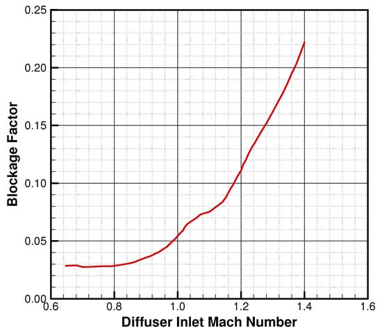
Figure 2.
Blockage factor versus the diffuser inlet Mach number.
It is concluded that to determine the throat and outlet areas, in addition to the mass flow rate and pipe count N, designers should provide the total temperature , total pressure , and Mach number at both the inlet and outlet of a pipe diffuser.
2.2. The Centerline
As indicated by the red line in Figure 3, the centerline of the fishtailed pipe diffuser can be divided into two segments: the radial–conical section and the radial-to-axial section. The former is a straight line, while the latter is represented by a spatial spline. The centerline can be designed based on the circumferential angle and metal angle distributions. The circumferential angle refers to the angle between the plane formed by the X-axis and the point (,,) on the centerline and the XOZ plane. The metal angle denotes the angle between this same plane and the tangent at the corresponding point (,,). An example is shown in Figure 4. The abscissa represents the normalized meridional length, while the ordinate represents the metal or circumferential angle.
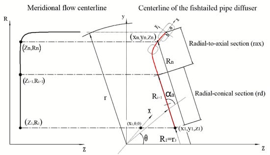
Figure 3.
Schematic of two centerlines.
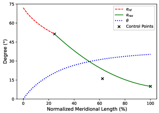
Figure 4.
Angle distributions versus normalized meridional length.
2.2.1. Radial–Conical Section
The centerline of the radial–conical section can be derived using the coordinates of the diffuser meridional flow path centerline ( and ), along with the diffuser inlet metal angle . It is crucial to ensure that the z-coordinate of the centerline remains constant throughout this section. The diffuser inlet angle is designed to align with the absolute exit flow angle of the impeller at the design operating point. This can be achieved by setting = to [10,18].
To obtain the Cartesian coordinates of the centerline, the corresponding circumferential angle distribution (blue dash line in Figure 4) must be determined. For the radial–conical section, the circumferential angle can be defined as follows:
where n represents the sequence number of the meridional flow path coordinates, with 1 denoting the diffuser inlet and i denoting the last point of the radial–conical section. Then, the Cartesian coordinates of the centerline for the radial–conical section can be derived as follows:
In addition, the metal angle distribution of the radial–conical section (red dash line in Figure 4) can be derived from ; that is .
2.2.2. Radial-to-Axial Section
The centerline of the radial-to-axial section can be determined based on the radial–conical section, the centerline coordinates of the diffuser meridional flow path ( and ), and the metal angle distribution . This distribution, which governs the metal angle along the diffuser’s centerline from the radial-to-axial section, can be controlled using a Bezier curve (green line in Figure 4). The starting point’s vertical coordinate aligns with the metal angle at the exit of the radial–conical section, given by , while the ending point’s vertical coordinate is determined based on the desired exit flow angle . The exit metal angle is defined as , where denotes the desired exit flow angle and represents the deviation angle ranging from 4° to 8° [13].
Based on the metal angle distribution , the circumferential angle of the radial-to-axial section can be determined:
The Cartesian coordinates of the centerline for the radial-to-axial section can be derived accordingly:
2.3. Cross-Sectional Area Distribution
The cross-sectional area distribution along the centerline can be divided into three segments: the throat section, the conical section, and the radial-to-axial section. Figure 5 illustrates an example of the normalized cross-sectional area distribution, with the abscissa representing the normalized meridional length and the ordinate representing the normalized cross-sectional area (normalized by the throat area; that is ).
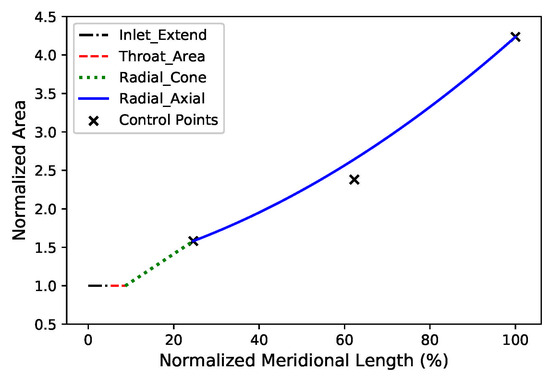
Figure 5.
Normalized area versus normalized meridional length.
1. Throat (Throat_Area in Figure 5): The first segment represents the region where the cross-sectional area remains constant, equal to the throat area , with its length defined as .
2. Conical section (Radial_Cone in Figure 5): The second segment requires consideration of the divergence angle of the radial expansion cone, so the area distribution in this section is linear.
3. Radial-to-axial section (Radial_Axial in Figure 5): The final segment is determined using a Bezier curve, the vertical coordinate of the starting point aligns with the normalized cross-sectional area at the exit of the conical section, and the ending point’s vertical coordinate is .
In addition to these three sections, Figure 5 includes a black dash dot line labeled Inlet_Extend. This section extends the throat area to facilitate the geometric modeling of the scalloped leading edge. Further details are provided in Section 2.5.
2.4. Cross Sections
The design of cross sections is guided by the fishtailed pipe diffuser’s centerline, area distribution, and the cross-sectional equation. In this paper, the equation of is utilized. The Cartesian coordinates are then determined as follows:
where denotes a point on the fishtailed pipe diffuser’s centerline, represents rounding to the nearest integer, and represents truncation, taking the integer part before the decimal point. The schematic of a cross-sectional profile with its geometric centroid explicitly marked is depicted in Figure 6. To ensure that the endpoints of the major axis or semi-major axis of the output cross-section are concentric with the center point, as shown in Figure 7, the unit vectors and must satisfy the following conditions:
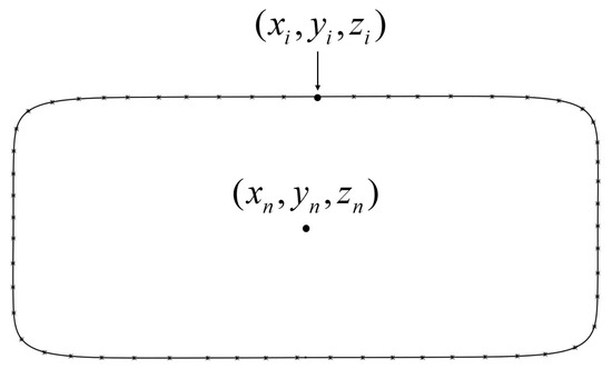
Figure 6.
Schematic of a cross-sectional profile.
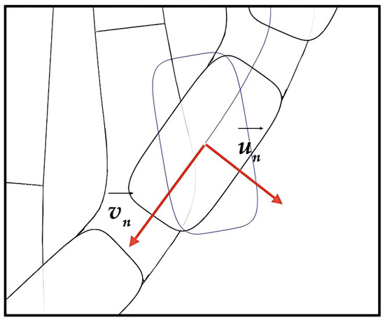
Figure 7.
Schematic of the exit cross section with various unit vectors.
Here, it is essential to explain the method for determining the equation . When , the cross-sectional shape forms a rhombus; when , it takes on a circular or elliptical shape; and when and , the shape becomes quasi-elliptical. As r and s increase, the cross-section gradually approaches a rectangular shape. It is recommended [12] that r and s range from 2 to 8 (or more). However, the optimal ranges for r and s have not yet been thoroughly explored or published.
Furthermore, it is necessary to determine the values of the major axis a and the semi-major axis b for the equation . One of these values, a or b, can be determined based on the width of the diffuser flow passage (such as the equivalent hydraulic diameter of throat, or ), while the other can be obtained based on the cross-sectional area. The area of a quasi-elliptical surface is proportional to that of an ellipse and can be expressed as follows:
Therefore, it is only necessary to determine the area coefficient for various r or s, as detailed in Appendix A. When r and s are non-integer values, the corresponding area coefficient can be obtained by interpolating the data.
2.5. Scalloped Leading Edge
Numerous studies [17,19,20] have highlighted the significance of the scalloped leading edge as a crucial feature of pipe diffusers. The structure, formed by the intersection of adjacent pipes, plays a pivotal role in influencing the performance of a diffuser. However, it is essential to adhere to specific design rules to ensure that the pipe diffuser effectively incorporates the scalloped leading edge.
Figure 8 illustrates the schematic diagram of the pipe diffuser with a scalloped leading edge, where (a) shows an overview and (b) offers a close-up. Figure 8b is included to clarify the derivation of coordinates B and G on the scalloped leading edge. Assuming the centerline of the pipe diffuser is aligned parallel to the X-axis, the corresponding tangent circle radius is . Points B and G represent the start and end points of the scalloped leading edge, respectively, as shown in Figure 1a,b. Therefore, as depicted in the figure, the scalloped leading edge forms when . According to the principle of similar triangles, the coordinates () corresponding to can be determined using the following formula:
where represents the equivalent hydraulic radius. Regarding , the corresponding coordinates can be expressed as follows:
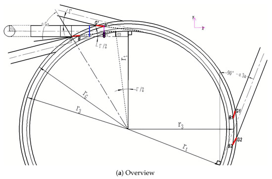
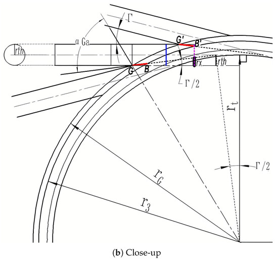
Figure 8.
Generalized pipe diffuser geometry with scalloped leading edges (planar projection).
By employing the aforementioned method, the projection line of the scalloped leading edge on the XOY plane can be determined. Subsequently, the coordinates of points B and G at various positions can be derived through coordinate transformation. For instance, considering the coordinates of points and in Figure 8b, the corresponding coordinates () and () can be calculated using the following formulas with the single passage angle :
To finish the geometric modeling of the scalloped leading edge (particularly leading edge ), the starting point of the pipe diffuser’s centerline should be located on the purple dashed line in Figure 8b. However, according to Equation (8), the starting point lies on the blue dash-dot line where the radial coordinate is . Therefore, it is recommended to employ the Inlet_Extend section. The radial coordinate of the new centerline’s starting point can be expressed as follows:
For the actual coordinates (such as (,) and (,) in this paper) and formulas of the scalloped leading edge in Figure 8a, please refer to Appendix B.
The inlet metal angle of the scalloped leading edge can be expressed as follows:
Subsequently, the incidence can be computed based on the inlet flow angle , which is as follows:
Following the aforementioned methodology, a fishtailed pipe diffuser can be designed, as exemplified in Figure 1b and Figure 9. Additionally, to facilitate numerical simulations, it is essential to incorporate a vaneless diffuser section between the impeller and the fishtailed pipe diffuser. This section can be generated by lofting between the impeller exit surface and the diffuser inlet surface, where the latter is formed by trimming the fishtailed pipe diffuser with the annular surface corresponding to .
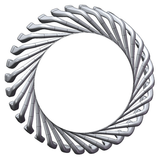
Figure 9.
Schematic of the fishtailed pipe diffuser model with vaneless diffuser.
3. The Fishtailed Pipe Diffuser for the NASA HECC Compressor
3.1. The NASA HECC Centrifugal Compressor Stage (Compressor A)
The NASA high-efficiency centrifugal compressor (HECC), referred to as Compressor A in this paper, featuring an unshrouded impeller, a vaned diffuser, and an exit guide vane (EGV), has been selected as the benchmark for this investigation. The NASA report indicates that both the impeller and the vaned diffuser incorporate splitters designed to alleviate flow separations. The positioning of the EGV relative to the vaned diffuser was examined with regard to the clocking effect. Figure 10 and Table 1 provide detailed illustrations of the compressor geometry and its design parameters, respectively.

Figure 10.
The NASA HECC stage. Reproduced with permission from Medic et al. Technical Report No.NASA/CR-218114, 2014. Copyright 2014 Publish Use Permitted [14].

Table 1.
Design parameters of the HECC stage.
3.2. The Fishtailed Pipe Diffuser (Compressor B)
Based on the geometric dimensions and aerodynamic parameters of the NASA HECC impeller exit, a new diffuser has been designed. The diffuser geometry is divided into two parts: one is the fishtailed pipe diffuser designed following the methodology presented in Section 2, while the other one is an extended duct. As illustrated in Figure 11, the centerline of the fishtailed pipe diffuser flow path is represented by a red line, with its end aligned with the trailing edge of the EGV. Downstream of this interface, the flow path transitions into an extended duct (shown in a green line). This segment serves as an aerodynamic continuation of the fishtailed pipe diffuser exit, ensuring that it maintains the same exit position of the NASA HECC exit. It is worth noting that both the prototype diffuser (spanning from the vaned diffuser to the EGV) and the fishtailed pipe diffuser maintain the same exit metal angle (approximately 3.17° at the EGV exit) and exit area [14]. The design parameters, centerline metal angle distribution, normalized area distribution, and the diffuser geometry (with the end duct) are detailed in Table 2, Figure 4, Figure 5, and Figure 9, respectively. In this paper, the HECC impeller configured with the new diffuser (referred to hereafter as the fishtailed pipe diffuser for convenience) is designated as Compressor B.
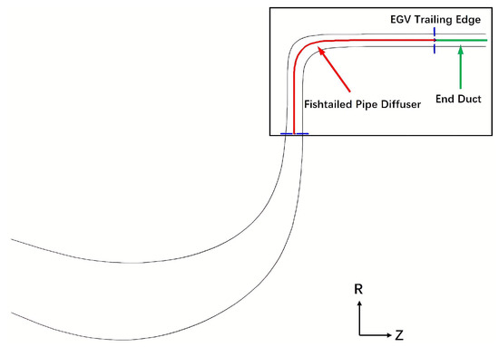
Figure 11.
Schematic of the new diffuser flow path centerline.
Table 2.
Design parameters of the fishtailed pipe diffuser geometry.
4. Numerical Setting-Up
4.1. Solver
Numerical analyses of the fishtailed pipe diffuser for the NASA HECC compressor (Compressor B) are performed using the commercial CFD software ANSYS CFX 2021 R1. A second-order spatial discretization scheme and high-resolution turbulence options are used. The pressure-based coupled algebraic multigrid method is employed, with pressure–velocity coupling handled by the Rhie and Chow momentum interpolation scheme [21] to prevent pressure oscillations. Furthermore, the viscous work term is included in the total energy equation to model internal heating by viscosity, which is necessary for cases involving multiple frames of reference (MFR), such as turbomachinery simulations.
4.2. Mesh
A full-hexahedral structured mesh for the NASA HECC impeller is generated using the commercial software NUMECA 13.2, AutoGridTM. Figure 12 illustrates a single passage mesh of the HECC impeller, including blade fillets in the geometry. The “butterfly” mesh topology is chosen to accurately capture the actual geometry of the fillets without compromising mesh quality. A fully tetrahedral unstructured mesh for the fishtailed pipe diffuser is generated using ANSYS ICEM CFD 2021 R1, as shown in Figure 13. The values on both the blade surfaces and end walls are maintained below 3.0.
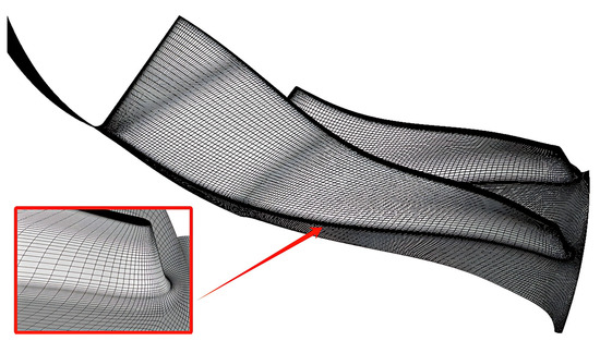
Figure 12.
HECC impeller mesh with fillets.
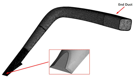
Figure 13.
The fishtailed pipe diffuser mesh.
4.3. Boundary Conditions
The boundary conditions are consistent with those described in reference [22]. At the inlet boundary, a fixed total pressure of 101,325 Pa and a total temperature of 293.15 K are specified, with the flow direction perpendicular to the inlet surface. The turbulence intensity is set to 1%, as mentioned in the NASA report [14]. Static pressure is specified at the exit boundary, and it is adjusted to simulate flow conditions from choke to near stall. Non-slip, adiabatic wall conditions are applied, along with an equivalent sand grain roughness of 9 μm on both the blade surfaces and end walls. The mixing plane interface with “constant total pressure” is used to connect the impeller and fishtailed pipe diffuser.
4.4. Grid Independence Study
A grid independence study is carried out using the Wilcox k-Omega () turbulence model [23], with the impeller grid fixed at 2.3 million cells. This configuration has already been validated in our previous work [22]. For the fishtailed pipe diffuser, three grids of varying densities (1.87 million, 2.64 million, 296, and 3.75 million cells) were employed for this analysis, building upon the baseline impeller mesh from [22]. To ensure consistency in the value, the first cell width on the diffuser wall is kept constant across all grids.
In Figure 14, the isentropic efficiency and total pressure ratio are plotted against the mass flow rate normalized by the measured choked flow of the prototype design [14]. It can be observed that the speedline obtained with 2.64 million grid nodes for the fishtailed pipe diffuser closely matches the results of the fine mesh case. Hence, utilizing the 2.64 million grid nodes for the fishtailed pipe diffuser provides an optimal balance between accuracy and computational cost.
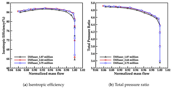
Figure 14.
Performance characteristics for different grids.
4.5. Comparison of Various Turbulence Models
Beyond the grid independence study, the reliability of the numerical simulations is further validated by assessing the impact of various turbulence models on Compressor B. In this study, four eddy viscosity turbulence models, namely Wilcox k-Omega (), Standard k-Epsilon () [24], Shear Stress Transport () [25], and SST-reattachment modification () [26], are employed.
The performance characteristics of Compressor B with different turbulence models are illustrated in Figure 15. It can be seen that all models demonstrate closely aligned predictions for both isentropic efficiency and total pressure ratio across the whole speedline, while revealing marginal discrepancies in the choked mass flow rate. The and models predict the lowest choked mass flow rate, while the model exhibits the largest choked mass flow rate among all models. Additionally, the performance curves indicated that the model predicts a significantly smaller stable flow range compared to the other models, which aligns with findings reported in reference [22]. Though there are some differences among these four models, the deviations of characteristics such as isentropic efficiency, total pressure ratio, and choked mass flow rate are all below 1%. Therefore, it is thought that the turbulence models have limited influence on the simulation results for Compressor B.
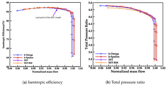
Figure 15.
Stage characteristics of the fishtailed pipe diffuser with various turbulence models.
Although there is a lack of experimental validation, the aforementioned work eliminates uncertainties related to grid independence and turbulence models, thereby ensuring the reliability of the numerical results. In this paper, the Wilcox k-Omega () turbulence model, which has shown good agreement with the test data for the NASA HECC compressor (Compressor A) [22], is selected to ensure consistency in comparisons between Compressor A and Compressor B.
5. Performance Characteristics
5.1. Overall Performance
Figure 16 illustrates the overall performance of Compressor A and Compressor B. The total-to-total isentropic efficiency and total pressure ratio are plotted versus the mass flow rate normalized by the measured choked mass flow rate of Compressor A. The experimental data of Compressor A is included in the figure for reference. It is seen that the isentropic efficiency and total pressure ratio curves for Compressor B exhibit an upward shift compared to Compressor A over the whole speedline, indicating a notable enhancement in aerodynamic performance. At the design operating point (near the green dashed line), the isentropic efficiency and total pressure ratio show an increase of 2.4 percentage points and 2.7%, respectively.
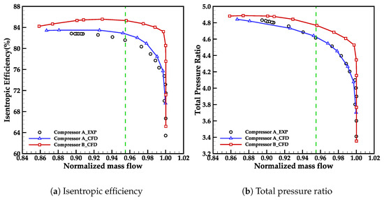
Figure 16.
Overall performance of Compressor A and Compressor B.
5.2. Impeller Performance
Figure 17 depicts the performance characteristics of the HECC impeller when integrated into Compressor A and Compressor B. Subfigures (a) and (b) represent the total-to-total isentropic efficiency and total pressure ratio of the HECC impeller versus the normalized mass flow rate, respectively. Subfigures (c) and (d) present the spanwise distributions of the total-to-total isentropic efficiency and total pressure ratio at the impeller exit, corresponding to the design operating point (near the green dashed line in Figure 17a,b).
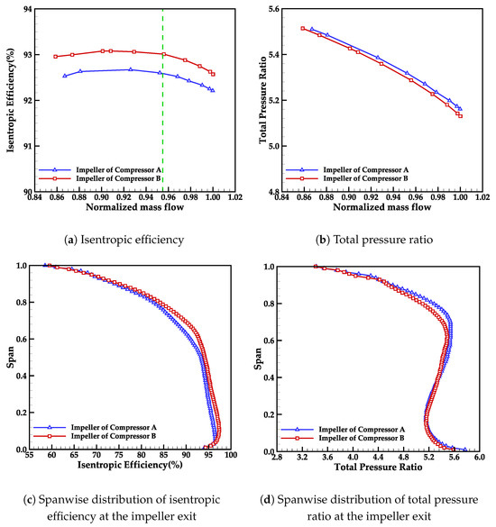
Figure 17.
The HECC impeller performance characteristics of Compressor A and Compressor B.
As shown in Figure 17a,b, the impeller in Compressor B consistently exhibits slightly higher isentropic efficiency and nearly identical total pressure ratio across the entire speedline compared to the impeller in Compressor A. Additionally, Figure 17c,d demonstrate that variation in efficiency almost originates from the entire spanwise, while difference in pressure ratio primarily stems from the upper midspan region of the impeller.
Although certain variations are observed, the results indicate that the impeller’s influence on the overall performance of both the Compressor A and Compressor B is relatively minor. The performance characteristics of the two HECC impellers suggest that the notable improvement in compressor efficiency is predominantly attributed to the superior performance of the fishtailed pipe diffuser (in Compressor B). In addition, the use of different diffusers in the compressors has a slight impact on the performance of the same impeller.
5.3. Diffuser Performance
The static pressure recovery () and total pressure loss () of the two different diffusers are shown in Figure 18. These two parameters are defined as follows:
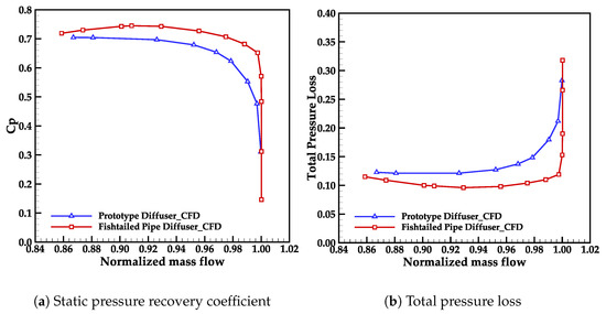
Figure 18.
Performance characteristics of two diffusers.
It is important to note that the position of station 3 deviates from that in references [14,22] due to the specific design dimensions of the fishtailed pipe diffuser. For the purpose of a fair comparison, the position of station 3 in the prototype design is aligned with that of the fishtailed pipe diffuser. It can be observed that the fishtailed pipe diffuser shows much higher values and lower compared to the prototype diffuser, revealing the significant performance enhancements primarily achieved with the fishtailed pipe diffuser.
5.4. Flow Mechanism in Two Diffusers
This section provides a detailed comparative analysis of the internal flow between the two different diffusers. To achieve a thorough evaluation, eleven stations are employed along the fishtailed pipe diffuser passage, as illustrated in Figure 19a. These cross-sections, labeled from station 1 to station 11, correspond to various regions within the fishtailed pipe diffuser. Specifically, station 1 and station 2 encompass the scalloped leading edge region. Station 2 and station 3 are positioned at the throat inlet and outlet, respectively. The radial–conical section of the fishtailed pipe diffuser is covered by station 3 to station 5, while station 5 to station 11 are evenly distributed along the radial-to-axial section.
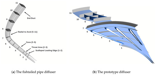
Figure 19.
Selected eleven stations of two diffusers.
For the prototype diffuser, the same stations are utilized, maintaining consistent radial dimensions within the radial–conical section (station 1 to station 5) and nearly consistent axial dimensions in the radial-to-axial section (station 6 to station 11), as depicted in Figure 19b. However, due to the unique structure of the fishtailed pipe diffuser, certain stations, such as those in the scalloped leading edge and throat area, are exclusive to the fishtailed pipe diffuser, whereas for the prototype diffuser, these stations are included purely for comparative analysis purposes.
Figure 20 presents the static pressure recovery coefficient (), specific entropy, and absolute Mach number profiles at eleven stations along the passage of the prototype diffuser and the fishtailed pipe diffuser configurations. The values are calculated with reference to the circumferentially area-averaged static pressure at the exit of the two HECC impellers. It is seen that both diffusers exhibit a similar trend in static pressure recovery. The non-zero value at the inlet of the fishtailed pipe diffuser is attributed to the position of station 1, which is located a certain distance away from the outlet section of the HECC impeller. The primary distinction in the distribution between these two diffusers occurs between station 2 and station 3. In the fishtailed pipe diffuser, the constant throat area between these stations, coupled with the developing boundary layer whose ongoing growth slightly reduces the effective flow area, leads to a slight increase in flow velocity (as shown in Figure 20c), causing a minor decrease in . Beyond station 4, the fishtailed pipe diffuser demonstrates a higher than the prototype diffuser, probably due to its capacity to mitigate flow separations or re-energize the low-momentum fluids. As previously noted, this performance enhancement is attributed to its scalloped leading edge. The incoming flow passing through this feature forms two pairs of counter-rotating vortices, which re-energizes and transport the flow while alleviating adverse effects from low-energy fluids. A detailed mechanism analysis will be presented in subsequent sections. Notably, both diffusers exhibit a decrease in at station 8, attributed to significant flow separation occurring after passing through the radial-to-axial region (between station 7 and station 8). The minor decrease in between station 10 and station 11 in the fishtailed pipe diffuser can be attributed to the friction losses over the equivalent surface area in the end duct.
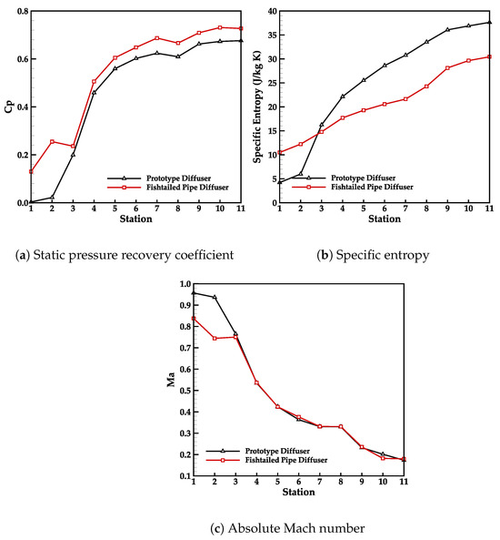
Figure 20.
Performance comparison of two diffusers.
Figure 20b indicates that the fishtailed pipe diffuser experiences a more gradual increase in entropy compared to the prototype diffuser. While the entropy values for both diffusers are nearly identical at station 3, the prototype diffuser suffers significantly higher losses after station 3, a trend that continues until reaching the compressor exit. In the region between station 7 and station 8, similar to the distribution, entropy for both diffusers rise due to flow separations induced by the bend. Additionally, it is observed that the flow separation in the fishtailed pipe diffuser remains unmitigated, resulting in an entropy increase trend similar to that observed in the prototype diffuser. Finally, according to Figure 20c, both diffusers show nearly identical exit Mach numbers when maintaining the same exit area.
Figure 21 and Figure 22 depict the non-dimensionalized entropy distributions along the selected stations for two diffusers, respectively. In the case of the fishtailed pipe diffuser, surface streamlines are included to track the evolution of vortices and energy transport within the passage. The entropy values have been non-dimensionalized using the compressor work input, as derived by Denton [27]. The corresponding formula is provided below:
where represents the heat capacity and S denotes entropy. At station 1, located in the pseudo-vaneless space of the fishtailed pipe diffuser, two counter-rotating vortices are generated near the pressure side (PS). The vortex near the shroud wall (VS) is dominant compared to the one near the hub wall (VH). This predominance occurs because the upstream vortex, which initially moves counter-clockwise from the hub towards the shroud wall, is influenced by varying incidences from the hub to the shroud span when encountering the scalloped leading edge ridge. Consequently, though the vortex divided into two parts, the VS maintains its dominant position.
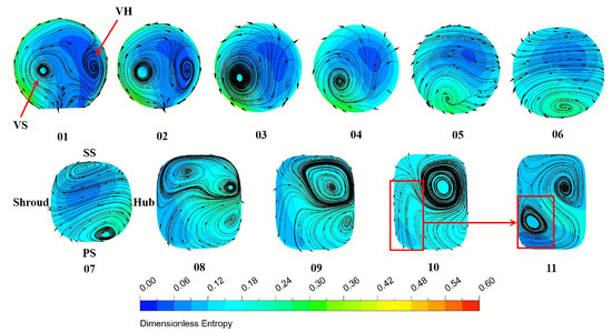
Figure 21.
Entropy distribution and streamlines at various stations in the fishtailed pipe diffuser.
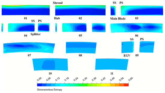
Figure 22.
Entropy distribution at various stations in the prototype diffuser.
From station 2 to station 6, it is observed that these two vortices, especially the VS, effectively transport both the high-energy and low-momentum flow near the PS into the main flow region, directing them along a counter-clockwise path near the diffuser wall towards the PS. This process re-energizes the low-momentum flow, leading to a reduction in aerodynamic loading and contributing to the improved performance of the fishtailed pipe diffuser. Additionally, a clockwise vortex is observed near the suction side (SS) at station 7 due to a combination of expansion-induced separation (highlighted as zone 1 in Figure 23) and abrupt curvature variations in the hub of the radial-to-axial region which causes a significant change in velocity direction. This vortex further deteriorates as the flow progresses. At station 8, two vortices are observed near the SS, occupying nearly half of the flow passage. As the flow progresses, these two vortices merge into a single large vortex, which then combines with the vortex near the PS, moving toward the compressor exit. From station 7 to station 11, the vortex near the PS continues to play a role in transporting and redistributing the fluid. This vortex ultimately merges with the vortex near the SS. At station 11, a new vortex near the PS is then generated. However, the ability to mitigate losses is weakened by upstream flow separations, which could be the primary reason for the reduced gradient in static pressure recovery after station 8.
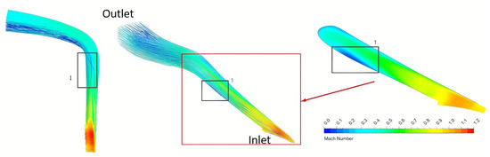
Figure 23.
Streamlines and Mach number distributions in the fishtailed pipe diffuser (left and middle: 3D streamlines; right: Mach number distribution on the midspan).
Figure 22 shows the normalized entropy distribution of the prototype diffuser. From station 1 to station 2, the high-entropy region is primarily concentrated near the shroud wall, driven by the tip leakage separation from the HECC impeller. Due to the effect of the negative incidence, a boundary layer flow separation is induced on the pressure side. According to what is observed in station 3, the low-momentum flow which causes high entropy can be observed near the main blade pressure side. This phenomenon is also observed in Figure 24. However, unlike the fishtailed pipe diffuser, the prototype diffuser struggles to effectively suppress flow separations or low-momentum flow, leading to further deterioration and increased losses compared to the fishtailed pipe diffuser. After passing through the vaned diffuser, the separated low-momentum fluid mixes with the main flow and continues towards the compressor exit.
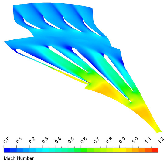
Figure 24.
Mach number contour at 10% span (prototype diffuser).
6. Conclusions
This paper presents a comprehensive design methodology for fishtailed pipe diffusers, aiming to fill the gap in the open literature. Based on the proposed methodology, a fishtailed pipe diffuser is developed for the NASA HECC centrifugal impeller. Numerical simulations demonstrate that the fishtailed pipe diffuser significantly enhances the aerodynamic performance of the compressor in terms of isentropic efficiency and total pressure ratio. These findings confirm the reliability and effectiveness of the proposed methodology. The main conclusions drawn from this study are as follows:
- The design of a fishtailed pipe diffuser can be systematically achieved using aerodynamic parameters, diffuser centerline, metal angle distribution, and area distribution. This methodology ensures both efficiency and reliability in a design process.
- At the design operating point, the fishtailed pipe diffuser increases the isentropic efficiency and the total pressure ratio by 2.4 percentage points and 2.7%, respectively.
- For the fishtailed pipe diffuser, a pair of counter-rotating vortices generated by the scalloped leading edge can transport and re-energize the low-momentum flow near the pressure side, effectively suppressing upstream flow separations. In constrast, the prototype vaned diffuser lacks the ability to redistribute low-energy fluid, leading to higher losses.
7. Discussion
It is noteworthy that this study reveals significant flow separation in the flow field of the fishtailed pipe diffuser, primarily concentrated around the radial-to-axial section. This phenomenon may stem from suboptimal design parameters, such as the radial–conical divergence angle , area distribution, and so on. Although some studies have been conducted in this area, the existing findings remain incomplete and fall short of detailed guidance on the design parameters of pipe diffusers. Further work will focus on investigating the impact of various design parameters on the performance of pipe diffusers, with the goal of achieving an optimized pipe diffuser design, aiming to provide comprehensive design guidelines and refine the fishtailed pipe diffuser design methodology presented in this paper.
8. Patents
The design methodology described in Section 2 has been embodied in an patent (CN 119026282 B, granted on 18 April 2025) [15].
Author Contributions
Conceptualization, J.L.; methodology, J.L.; software, J.L.; validation, J.L.; formal analysis, J.L., D.W. and X.H.; investigation, J.L.; data curation, J.L.; writing—original draft preparation, J.L.; writing—review and editing, J.L., D.W. and X.H.; supervision, D.W. and X.H. All authors have read and agreed to the published version of the manuscript.
Funding
This research received no external funding.
Data Availability Statement
The data supporting the results of this study are available in the NASA publicly archived datasets, accessible via the following link, accessed on 28 March 2022, https://ntrs.nasa.gov/citations/20180001471.
Conflicts of Interest
The authors declare no conflicts of interest.
Nomenclature
| A | Area, |
| b | 1) Blade height, m 2) semi-major axis |
| B | Blockage factor |
| c | Ratio of throat length to throat diameter |
| Static pressure recovery coefficient | |
| d | Equivalent hydraulic diameter, m |
| i | Incidence, ° |
| K | Continuity equation constant |
| m | Meridional length, m |
| Mass flow rate, | |
| Absolute Mach number | |
| N | Number of pipes |
| p | Pressure, |
| q | Mass flux density gas-dynamic function |
| r | 1) Radius, m 2) exponent of the major axis of the quasi-elliptic equation |
| R | Radial coordinate of meridional flow path, m |
| s | Exponent of the semi-major axis of the quasi-elliptic equation |
| T | Temperature, K |
| x | X-coordinate, m |
| y | Y-coordinate, m |
| z | Z-coordinate, m |
| Z | Z-coordinate of meridional flow path, m |
| Abbreviations | |
| Total pressure loss | |
| SS | Suction side |
| PS | Pressure side |
| VS | Vortex near the shroud wall |
| VH | Vortex near the hub wall |
| Greek Symbols | |
| Absolute flow angle/metal angle (angles relative to the meridional plane), ° | |
| Relative flow angle (angles relative to the meridional plane), ° | |
| Deviation angle, ° | |
| 1) Divergence angle, ° 2) Circumferential angle, ° | |
| Velocity coefficient | |
| Total pressure loss coefficient | |
| Ratio of specific heats | |
| Single passage angle, ° | |
| Area coefficient | |
| Subscripts | |
| 2 | Impeller outlet |
| 3 | Diffuser inlet |
| 4 | Diffuser outlet |
| B | Scalloped leading edge point (start) |
| Pipe diffuser (single passage) | |
| Radial-to-axial section | |
| G | Scalloped leading edge point (end) |
| Diffuser/compressor outlet | |
| Radial–conical section | |
| t | Tangent |
| Throat area | |
| Superscripts | |
| * | Stagnation |
Appendix A
Table A1.
Area coefficient versus various r and s.
Table A1.
Area coefficient versus various r and s.
| s | 2 | 3 | 4 | 5 | 6 | 7 | 8 | 9 | |
|---|---|---|---|---|---|---|---|---|---|
| r | |||||||||
| 2 | 1 | 1.0712 | 1.1129 | 1.1402 | 1.1596 | 1.1740 | 1.1852 | 1.1941 | |
| 3 | 1.0712 | 1.1247 | 1.1555 | 1.1758 | 1.1902 | 1.2008 | 1.2090 | 1.2155 | |
| 4 | 1.1129 | 1.1555 | 1.1803 | 1.1964 | 1.2077 | 1.2162 | 1.2226 | 1.2281 | |
| 5 | 1.1402 | 1.1758 | 1.1964 | 1.2097 | 1.2192 | 1.2263 | 1.2315 | 1.2359 | |
| 6 | 1.1596 | 1.1902 | 1.2077 | 1.2192 | 1.2274 | 1.2332 | 1.2378 | 1.2415 | |
| 7 | 1.1740 | 1.2008 | 1.2162 | 1.2263 | 1.2332 | 1.2383 | 1.2424 | 1.2455 | |
| 8 | 1.1852 | 1.2090 | 1.2226 | 1.2315 | 1.2378 | 1.2424 | 1.2459 | 1.2486 | |
| 9 | 1.1941 | 1.2155 | 1.2281 | 1.2359 | 1.2415 | 1.2455 | 1.2486 | 1.2512 | |
Appendix B. Coordinates of the Scalloped Leading Edge
References
- Vrana, J.C. Diffuser for Centrifugal Compressor. U.S. Patent 3333762, 1 August 1967. [Google Scholar]
- Kenny, D.P. A novel low-cost diffuser for high-performance centrifugal compressor. J. Eng. Power 1969, 91, 37–46. [Google Scholar] [CrossRef]
- Zachau, U.; Buescher, C.; Niehuis, R. Experimental investigation of a centrifugal compressor stage with focus on the flow in the pipe diffuser supported by particle image velocimetry (piv) measurements. In Proceedings of the ASME Turbo Expo 2008: Power for Land, Sea and Air, Berlin, Germany, 9–13 June 2008. [Google Scholar]
- Bourgeois, J.A. Experimental and numerical investigation of an aero-engine centrifugal compressor. In Proceedings of the ASME Turbo Expo 2009: Power for Land, Sea and Air, Orlando, FL, USA, 8–12 June 2009. [Google Scholar]
- Han, G.; Lu, X.G.; Zhao, S.F.; Yang, C.W.; Zhu, J.Q. Parametric studies of pipe diffuser on performance of a highly loaded centrifugal compressor. J. Eng. Gas. Turb. Power 2014, 136, 122604. [Google Scholar] [CrossRef]
- Erickson, D.W. Characterization and impact of secondary flows in a discrete passage centrifugal compressor diffuser. In Proceedings of the ASME Turbo Expo 2018: Turbomachinery Technical Conference and Exposition, Oslo, Norway, 11–15 June 2018. [Google Scholar]
- Han, G.; Lu, X.G.; Zhang, Y.F.; Zhao, S.F.; Yang, C.W.; Zhu, J.Q. Investigation of two pipe diffuser configurations for a compact centrifugal compressor. Proc. Inst. Mech. Eng. Part G J. Aerosp. Eng. 2018, 232, 716–728. [Google Scholar] [CrossRef]
- Ogino, A.; Nakayama, R.; Kitamura, E.; Fujisawa, N.; Aoyama, S.; Ohta, Y. Diffuser stall inception in a high-pressure ratio centrifugal compressor with fishtail pipe diffuser. In Proceeding of the ASME Turbo Expo 2023: Turbomachinery Technical Conference and Exposition, Boston, MA, USA, 26–30 June 2023. [Google Scholar]
- Bennett, I. The Design and Analysis of Pipe Diffusers for Centrifugal Compressors. Ph.D. Thesis, Cranfield University, Cranfield, UK, 1997. [Google Scholar]
- Antas, S. Pipe diffuser for radial and axial-centrifugal compressor. Int. J. Turbo. Jet. Eng. 2014, 31, 29–36. [Google Scholar] [CrossRef]
- Wang, B.; Yan, M. Design and numerical simulation of pipe diffuser in centrifugal compressor. J. Aerosp. Power 2012, 27, 1303–1311. [Google Scholar]
- Antas, S. Exhaust system for radial and axial-centrifugal compressor with pipe diffuser. Int. J. Turbo. Jet. Eng. 2016, 36, 297–304. [Google Scholar] [CrossRef]
- Xie, J.; He, X.; Jin, H.L.; Chen, X.; Yin, Y.Q.; Huang, S.Q. Design Methodology for the Pipe Diffuser and Pipe Diffuser. CN Patent CN110374928A, 25 October 2019. [Google Scholar]
- Medic, G.; Shrama, O.P.; Jongwook, J.; Hardin, L.W.; McCormick, D.C.; Cousins, W.T.; Lurie, E.A.; Shabbir, A.; Holley, B.M.; Van Slooten, P.R. High Efficiency Centrifugal Compressor for Rotorcraft Application, NASA/CR-2014-218114; National Aeronautics and Space Administration: Washington, DC, USA, 2014. [Google Scholar]
- Liu, J.; Wang, D.X.; Huang, X.Q. A Design Methodology for the Fishtailed Pipe Diffuser with Scalloped Leading Edge. CN Patent CN119026282B, 18 April 2025. [Google Scholar]
- Wang, X. Fundamentals of Gas Dynamics, 2nd ed.; Northwestern Polytechnical University: Xi’an, China, 2006. (In Chinese) [Google Scholar]
- Kenny, D.P. A comparison of the predicted and measured performance of high pressure ratio centrifugal compressor diffusers. In Proceedings of the ASME International Gas Turbine and Fluids Engineering Conference and Products Show, San Francisco, CA, USA, 26–30 March 1972. [Google Scholar]
- Casey, M.; Robinson, C. Radial Flow Turbocompressors: Design, Analysis, and Applications; Cambridge University: Cambridge, UK, 2021. [Google Scholar]
- Han, G.; Yang, C.; Wu, S.; Zhao, S.F.; Lu, X.G. The investigation of mechanism on pipe diffuser leading edge vortex generation and development in centrifugal compressor. Appl. Therm. Eng. 2023, 219, 119606. [Google Scholar] [CrossRef]
- Wang, Y.; Zhao, S.F.; Lu, X.G.; Zhu, J.Q. Analysis of characteristic and mechanism of pipe diffuser for a highly loaded centrifugal compressor. J. Aerosp. Power 2011, 26, 649–655. [Google Scholar]
- Rhie, C.M.; Chow, W.L. A numerical study of the turbulence flow past on the airfoil with trailing edge separation. J. AIAA 1983, 21, 1525–1532. [Google Scholar] [CrossRef]
- Liu, J.N.; Wang, D.X.; Huang, X.Q. Investigation of turbulence models for areodynamic analysis of a high pressure ratio centrifugal compressor. Phys. Fluids 2023, 35, 106108. [Google Scholar] [CrossRef]
- Wilcox, D.C. Turbulence Modeling for CFD; DCW Industries: San Diego, CA, USA, 2006; pp. 124–136. [Google Scholar]
- Jone, W.P.; Launder, B.E. The calculation of low-reynolds-number phenomena with a two-equation model for turbulence. Int. J. Heat Mass. Tran. 1973, 16, 1119–1130. [Google Scholar] [CrossRef]
- Menter, F.R. Two-equation eddy-viscosity turbulence models for engineering applicaitons. J. AIAA 1994, 32, 1598–1605. [Google Scholar] [CrossRef]
- Bourgeois, J.A.; Martinuzzi, R.J.; Savory, E.; Zhang, C.; Roberts, D.A. Assessment of turbulence model predictions for an aero-engine centrifugal compressor. J. Turbomach. 2011, 133, 011025. [Google Scholar] [CrossRef]
- Denton, J.D. The 1993 IGTI scholar lecture: Loss mechanisms in turbomachines. J. Turbomach. 1993, 115, 621–656. [Google Scholar] [CrossRef]
Disclaimer/Publisher’s Note: The statements, opinions and data contained in all publications are solely those of the individual author(s) and contributor(s) and not of MDPI and/or the editor(s). MDPI and/or the editor(s) disclaim responsibility for any injury to people or property resulting from any ideas, methods, instructions or products referred to in the content. |
© 2025 by the authors. Licensee MDPI, Basel, Switzerland. This article is an open access article distributed under the terms and conditions of the Creative Commons Attribution (CC BY) license (https://creativecommons.org/licenses/by/4.0/).