Reentry Trajectory Online Planning and Guidance Method Based on TD3

Abstract

Aiming at the problem of poor autonomy and weak time performance of reentry trajectory planning for Reusable Launch Vehicle (RLV), an online reentry trajectory planning and guidance method based on Twin Delayed Deep Deterministic Policy Gradient (TD3) is proposed. In view of the advantage that the drag acceleration can be quickly measured by the airborne inertial navigation equipment, the reference profile adopts the design of the drag acceleration–velocity profile in the reentry corridor. In order to prevent the problem of trajectory angle jump caused by the unsmooth turning point of the section, the section form adopts the form of four multiple functions to ensure the smooth connection of the turning point. Secondly, considering the advantages of the TD3 dual Critic network structure and delay update mechanism to suppress strategy overestimation, the TD3 algorithm framework is used to train multiple strategy networks offline and output profile parameters. Finally, considering the reentry uncertainty and the guidance error caused by the limitation of the bank angle reversal amplitude during lateral guidance, the networks are invoked online many times to solve the profile parameters in real time and update the profile periodically to ensure the rapidity and autonomy of the guidance command generation. The TD3 strategy networks are trained offline and invoked online many times so that the cumulative error in the previous guidance period can be eliminated when the algorithm is called again each time, and the online rapid generation and update of the reentry trajectory is realized, which effectively improves the accuracy and computational efficiency of the landing point.

1. Introduction

The Reusable Launch Vehicle (RLV) [1,2] uses aerodynamic lift for the return to reentry. Compared with ballistic reentry, it has significant advantages such as strong lateral maneuverability, high landing point accuracy, controllable overload, and heat flow peak. It is a key technical way to achieve high-precision fixed-point return and flexible space use. However, the reentry process faces severe process constraints and terminal constraints, and the flight environment changes dynamically and has significant uncertainties, which pose a great challenge to online generation of feasible trajectories and guidance. Therefore, reentry trajectory planning and guidance algorithms have received extensive attention.

RLV reentry trajectory planning and guidance algorithms [3] mainly include nominal trajectory tracking guidance, predictor–corrector guidance [4,5], and intelligent guidance. In view of the fact that drag acceleration can quickly calculate flight range and can be quickly measured by airborne inertial navigation equipment, nominal trajectory tracking guidance using drag acceleration profile as the nominal trajectory has certain advantages. In order to ensure that the trajectory satisfies all flight constraints, it is necessary to transform the process constraints into the reentry corridor and plan the drag acceleration–velocity profile [6,7] in the reentry corridor. At the same time, for the time-controllable reentry flight problem, a fast trajectory planning method based on the drag acceleration-energy profile is proposed, which makes the time greatly adjustable and realizes the rapid prediction of the flight capability boundary. In order to obtain the drag acceleration-energy profile that meets the requirements of the flight range, References [8,9] used a multi-segment linear function to set the drag acceleration profile as a parameterized form, and then used the prediction–correction method to solve the parameters to obtain a standard trajectory. However, the turning point of the linear function is not smooth, which is not conducive to tracking guidance. In Reference [10], the reciprocal profile was described by a cubic spline function, and the smooth trajectory was generated quickly. The traditional standard trajectory guidance relies on the nominal trajectory and has been successfully applied to the space shuttle, but the flexibility is limited, and it is difficult to meet the requirements of future aircraft autonomy. Numerical predictor–corrector guidance relies on iterative numerical integration, which has low computational efficiency and is difficult to meet real-time application requirements. Therefore, it is urgent to develop online trajectory planning and guidance algorithms.

With the development of artificial intelligence, intelligent guidance has proposed new solutions to the above problems. The core of intelligent guidance is to use artificial intelligence (AI) technology, especially machine learning (ML), deep learning (DL), reinforcement learning (RL), and intelligent optimization algorithms, to give the reentry guidance system stronger perception, learning, decision-making, and adaptability. In References [11,12], a reentry guidance method based on reinforcement learning is proposed. It adopts the decoupling design idea of longitudinal and lateral guidance, and uses reinforcement learning to output the amplitude of the bank angle, which has considerable computational efficiency and higher terminal accuracy and robustness. Attempting to solve the problem of long generation time of predictive correction guidance commands, Reference [13] introduced a deep deterministic policy gradient (DDPG) combined with the flight profile generated by quasi-balanced flight conditions. Through the design of reinforcement learning reward function and the adjustment of guidance period, the problem of non-convergence of results caused by sparse reward in the process of deep reinforcement learning training is solved so that the aircraft can complete flight tasks with process constraints and terminal constraints. In order to improve the flight potential of the aircraft, Reference [14] used Proximal Policy Optimization (PPO) and TD3 algorithms to train reinforcement learning agents, output angle of attack and bank angle instructions, and improve the adaptability of the aircraft. Considering the influence of the no-fly zone, References [15,16] proposed a step-by-step intelligent guidance research framework of predictive correction guidance-pre-trained bank angle guidance model based on supervised learning-further upgraded bank angle guidance model based on reinforcement learning, which gets rid of the constraints of the traditional predictive corrector guidance method on the bank angle solution space, and expects to produce a better fly-around strategy.

In this paper, the pre-reentry trajectory is obtained by numerical integration of the dynamic equation after selecting the constant angle of attack and the bank angle. On the premise of pre-setting the angle of attack profile, the process constraints are converted into reentry corridors, and four multiple-function drag acceleration reference profiles are designed for the glide trajectory. According to the principle of profile continuity and smoothness, the profile parameters are simplified. Secondly, by offline training multiple TD3 strategy networks, a hierarchical reward is designed to meet the needs of the flight range, and the parameters of different nodes in the profile are solved, respectively. At the same time, through the longitudinal guidance of the tracking of the drag acceleration profile, the bank angle command is solved; lateral guidance is performed by tilting angle reversal to limit heading angle deviation. According to the current state and flight range of each drag acceleration profile node, the TD3 strategy networks are invoked multiple times online to plan the trajectory and update the profile periodically. By combining it with tracking guidance, the cumulative error in the previous guidance period can be eliminated when the algorithm is invoked again each time, which effectively improves the accuracy and computational efficiency of the landing point and realizes the online rapid generation and update of the reentry trajectory.

2. Reentry Modeling and Constraints

Ignoring the Earth’s oblateness, considering the Earth’s rotation, and taking time as the independent variable, the 3-DOF reentry dynamic model [6] of RLV is as follows:

$$\left\{\begin{array}{l}\dot{r}=V\sin \gamma \\ \dot{\lambda }={\displaystyle \frac{V\cos \gamma \cos \varphi }{r}}\\ \dot{l}={\displaystyle \frac{V\cos \gamma \sin \varphi }{r\cos \lambda }}\\ \dot{V}=-{\displaystyle \frac{D}{m}}-g\sin \gamma +{\tilde{C}}_V\\ \dot{\gamma }={\displaystyle \frac{1}{V}}\left({\displaystyle \frac{L\cos \sigma }{m}}-g\cos \gamma +{\displaystyle \frac{V^2\cos \gamma }{r}}\right)+{\tilde{C}}_{\gamma }\\ \dot{\varphi }={\displaystyle \frac{1}{V}}\left({\displaystyle \frac{L\sin \sigma }{m\cos \gamma }}+{\displaystyle \frac{V^2\cos \gamma \tan \lambda \sin \varphi }{r}}\right)+{\tilde{C}}_{\varphi }\end{array}\right.$$

(1)

$$\left\{\begin{array}{l}{\tilde{C}}_V={\omega }_e^{2}r{\cos }^2\lambda \sin \gamma -{\omega }_e^{2}r\cos \lambda \sin \lambda \cos \varphi \cos \gamma \\ {\tilde{C}}_{\gamma }=2{\omega }_e\cos \lambda \sin \varphi +{\displaystyle \frac{{\omega }_e^{2}r\left({\cos }^2\lambda \cos \gamma -\cos \lambda \sin \lambda \cos \varphi \sin \gamma \right)}{V}}\\ {\tilde{C}}_{\varphi }={\displaystyle \frac{{\omega }_e^{2}r\cos \lambda \sin \lambda \sin \varphi }{V\cos \gamma }}-{\displaystyle \frac{2{\omega }_e\left(\cos \lambda \cos \varphi \sin \gamma -\sin \lambda \cos \gamma \right)}{\cos \gamma }}\\ \end{array}\right.$$

(2)

where $r$ is the geocentric distance, $\lambda$ is latitude, $l$ is longitude, $V$ is the velocity of the aircraft relative to the Earth, $m$ is the mass of the aircraft, $\gamma$ is the track angle of the track, $\varphi$ is the azimuth of the track (positive in the north by west), $g$ is the acceleration of gravity, $\sigma$ is the bank angle, and ${\omega }_e$ is the angular velocity of the Earth’s rotation. ${\tilde{C}}_V$, ${\tilde{C}}_{\gamma }$, and ${\tilde{C}}_{\varphi }$ are the accelerations generated by the rotation of the Earth. $D$ and $L$ are the drag and lift of the aircraft.

Assuming that the Earth is an ideal sphere, the calculation formula of the flight height of the aircraft is as follows:

$$h=r-R_e$$

(3)

where $R_e$ is the average radius of the Earth.

In order to ensure that the aircraft successfully completes the reentry mission, the core constraints that the aircraft needs to meet during the reentry process mainly include process constraints, control constraints, and terminal constraints.

The process constraints [7] are mainly divided into heat flow constraint, overload constraint, dynamic pressure constraint, and equilibrium glide constraint (QEGC) when the bank angle is 0. The formula is

$$\dot{Q}=K_Q\sqrt{\rho }{V}^{3.15}\le {\dot{Q}}_{\max }$$

(4)

$$n_z=(L\cos \alpha +D\sin \alpha )/\mathrm{mg}\le n_{z\cdot \max }$$

(5)

$$\overline{q}=\rho V^2/2\le {\overline{q}}_{\max }$$

(6)

$$g-V^2/r-L\le 0$$

(7)

where $\alpha$ is the angle of attack, $\dot{Q}$ is the heat flux rate, $K_Q$ is the heat transfer coefficient, $n_z$ is aerodynamic overload, and $\overline{q}$ is dynamic pressure.

The control variables of the aircraft are the angle of attack and the bank angle. In the trajectory optimization, its amplitude needs to be constrained. The formula is

$$\left\{\begin{array}{l}\left|\alpha \right|\le {\alpha }_{\max }\\ \left|\sigma \right|\le {\sigma }_{\max }\end{array}\right.$$

(8)

where ${\alpha }_{\max }$ and ${\sigma }_{\max }$ are the maximum values of the angle of attack and the bank angle.

The terminal constraints of an aircraft generally include altitude, velocity, latitude, and longitude constraints, which can be expressed as

$$\left\{\begin{array}{l}V(t_f)=V_f\\ H(t_f)=H_f\\ \lambda (t_f)={\lambda }_f\\ l(t_f)=l_f\end{array}\right.$$

(9)

where $t_f$ is the terminal moment, $V_f$ is the terminal velocity, $H_f$ is the terminal height, ${\lambda }_f$ is the terminal latitude, and $l_f$ is the terminal longitude.

3. Rapid Planning of Reentry Trajectory in Drag Acceleration–Velocity Profile

3.1. Angle of Attack Profile and Reentry Corridor

1.

Angle of attack profile

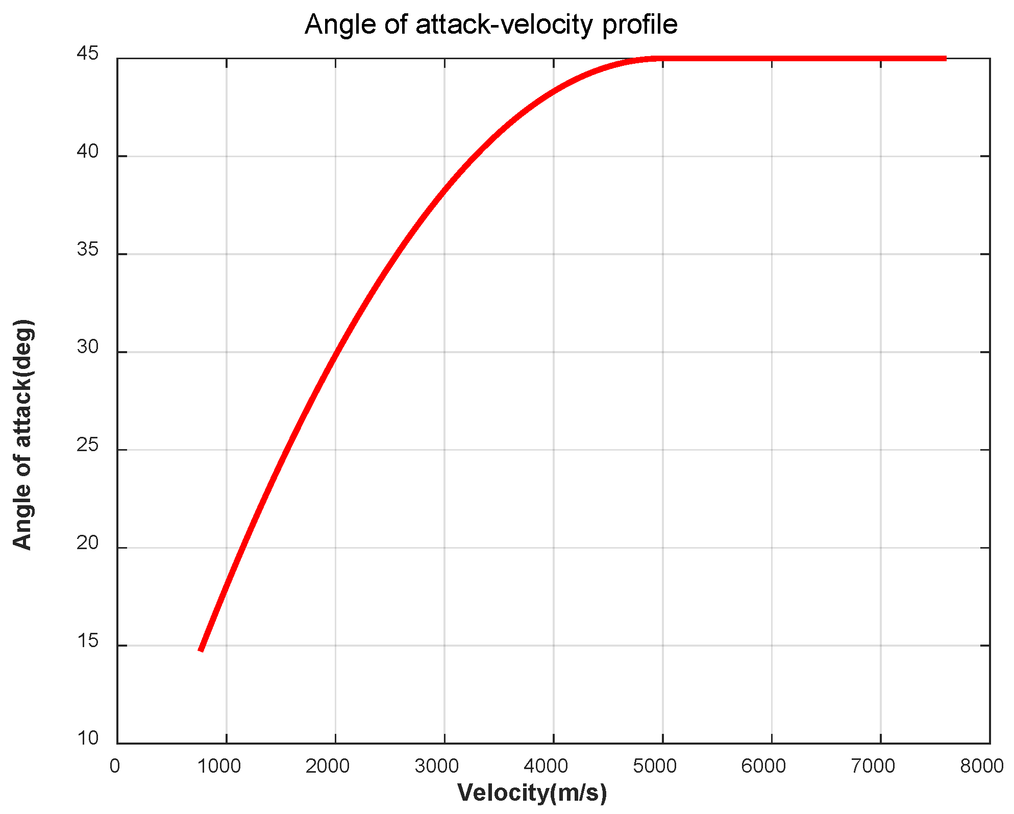
The angle of attack profile ($\alpha -V$) is a function of angle of attack with respect to velocity. At the beginning of reentry, RLV needs to fly at a high angle of attack to increase lift and drag, so as to avoid excessive heat flow caused by excessive height drop. With the decrease in speed and height, the angle of attack should be gradually reduced to reduce the lift and drag, which can avoid the jump of the trajectory caused by excessive lift, and can also reduce the drag and increase the range. When the reentry phase is coming to an end, in order to ensure that the RLV can perform guidance tracking in the energy management phase, it is necessary to transition the angle of attack to the front end of the maximum lift-to-drag ratio [7].

According to the above design principles, this paper refers to the angle of attack profile planning method of the space shuttle. At the beginning of reentry, it keeps flying at a high angle of attack. When the velocity is less than a certain value, the angle of attack begins to decrease with the velocity until it reaches the maximum lift-to-drag ratio at the end of reentry. In order to ensure the smooth connection of the subsequent track angle curve, the designed angle of attack–velocity profile formula is as follows:

$$\alpha (V)=\left\{\begin{array}{ll}45& V\ge 5000\\ a_{\alpha }{V}^2+b_{\alpha }V+c_{\alpha }& else\end{array}\right.$$

(10)

$$\left\{\begin{array}{l}{a}_{\alpha }\ast {5000}^2+b_{\alpha }\ast 5000+c_{\alpha }=45\\ a_{\alpha }{V_f}^2+b_{\alpha }{V}_f+c_{\alpha }=15\\ -b_{\alpha }/2a_{\alpha }=5000\end{array}\right.$$

(11)

where ${\alpha }_{\alpha }$, $b_{\alpha }$, and $c_{\alpha }$ are design parameters.

The angle of attack profile designed in this paper is shown in Figure 1.

2.

Reentry corridor

The calculation method of the reentry corridor is to convert the multiple process constraints into the constraints of a single physical quantity through a series of mathematical transformations [17]. The three process constraints of heat flow, overload, and dynamic pressure form the hard constraints of the reentry corridor, and QEGC forms the soft constraints of the reentry corridor, which together form the upper and lower boundaries of the reentry corridor.

The expression transformed from Equation (4) to Equation (7) into the drag acceleration–velocity corridor is

$$\left\{\begin{array}{l}D{a}_{\dot{Q}}={({\displaystyle \frac{{\dot{Q}}_{\max }}{K_Q{V}^{2.15}}})}^2{C}_{D}S/(2m)\\ D{a}_{n_z}={\displaystyle \frac{n_{z\max }g}{\frac{C_L}{C_D}\cos \alpha +\sin \alpha }}\\ D{a}_{\overline{q}}={\displaystyle \frac{{\overline{q}}_{\max }{C}_{D}S}{m}}\\ D{a}_{eg}=(g-{\displaystyle \frac{V^2}{r}}){\displaystyle \frac{C_D}{C_L}}\end{array}\right.$$

(12)

$$D{a}_{eg}\le Da(V)\le \min (D{a}_{\dot{Q}},D{a}_{n_z},D{a}_{\overline{q}})$$

(13)

where $D{a}_{\dot{Q}}$, $D{a}_{n_z}$, $D{a}_{\overline{q}}$, and $D{a}_{eg}$ are the drag acceleration boundaries corresponding to ${\dot{Q}}_{\max }$, $n_{z\max }$, ${\overline{q}}_{\max }$, and QEGC constraints, respectively. $Da(V)$ is the drag acceleration reference profile.

It is assumed that the overall constraint of RLV is as follows: the maximum heat flux rate is ${\dot{Q}}_{\max }=3000 \mathrm{kw}/{\mathrm{m}}^2$; the maximum overload is $n_{z\max }=3$; and the maximum dynamic pressure is ${\overline{q}}_{\max }=50 \mathrm{kpa}$. The corresponding relationship between the drag acceleration and the relative velocity is calculated by Equation (12), and the reentry corridor of the drag acceleration–velocity profile can be calculated, as shown in Figure 2. $D{a}_{\dot{Q}}$, $D{a}_{n_z}$, and $D{a}_{\overline{q}}$ together constitute the lower boundary of the height–velocity corridor, and $D{a}_{eg}$ forms the upper boundary of the height–velocity corridor.

3.2. Reentry Drag Acceleration Reference Trajectory Designing

The reentry trajectory of an unpowered RLV is usually divided into a pre-reentry section and a glide section [18]. The pre-reentry section is usually located at 60–120 km above sea level. In this stage, the atmospheric density is very thin, and the aerodynamic effect is not obvious. It is difficult for the spacecraft to adjust its trajectory by aerodynamic force. Therefore, it is usually necessary to maintain a constant large angle of attack and bank angle flight. When the spacecraft enters the glide phase, as the height decreases, the aerodynamic force begins to play a role, and the aircraft gradually generates guidance capability. At this time, the aerodynamic force can be used to achieve the purpose of adjusting the reentry trajectory, so this phase becomes the key link of reentry trajectory planning.

• Pre-reentry section

When the spacecraft is flying in the rarefied atmosphere, the aerodynamic force is weak, the aircraft has no guidance ability, and the control quantity has little effect on the descent trajectory. It can be considered that the spacecraft makes free-fall motion in this stage. Therefore, the angle of attack and bank angle in the pre-reentry section can be taken as constant ${\alpha }_0$ and ${\sigma }_0$. The reentry trajectory in the pre-reentry section is obtained by numerical integration of the dynamic Equation (1) [18].

The conditions for the end of the pre-reentry section are set as follows:

$$n_z\ge \delta$$

(14)

where $\delta$ is a small quantity pre-set according to the accuracy requirement.

The reason why Equation (14) is used as the end condition of the pre-reentry trajectory is that as the RLV enters the dense atmosphere from the thin atmosphere, when the overload reaches a certain value, the spacecraft can rely on aerodynamic force to change its flight trajectory, and the aircraft gradually has the ability to change the trajectory.

2.

Glide section

The glide section needs to carry out segmented trajectory design, which is generally composed of four sections [7]: temperature control section, equilibrium glide section, constant resistance section, and transition section. In order to ensure a smooth connection of each section, the first or second order function is selected for profile design. The drag acceleration–velocity expression of each stage is given below.

• Temperature control section: Ensure that the aircraft passes through the high heat flux area safely, starting from the end of the pre-reentry section until the maximum heat flux peak appears.

$$Da(V)=b_{1}V+c_1 \mathrm{if} V_1<V\le V_{yz}$$

(15)

• Equilibrium glide section: Establish a larger overload as soon as possible.

$$Da(V)=a_2{V}^2+b_{2}V+c_2 else if{V}_2<V\le V_1$$

(16)

• Constant resistance section: Maintain a large overload so that the aircraft has better maneuverability.

$$Da(V)=c_3 else if{V}_3<V\le V_2$$

(17)

• Transition section: By adjusting the velocity corresponding to the start of the transition section, the whole range can be adjusted more accurately.

$$Da(V)=a_4{V}^2+b_{4}V+c_4 else{V}_f<V\le V_3$$

(18)

where $b_1$, $c_1$, $a_2$, $b_2$, $c_2$, $a_4$, $b_4$, and $c_4$ are trajectory design parameters. $V_{yz}$, $V_1$, $V_2$, $V_3$, and $V_f$ are the terminal velocities of each section of the pre-reentry section and the gliding section.

According to Equations (15)–(18), there are 9 design parameters of the reference section. If the direct design is very complicated and not intuitive, and if the endpoints of each section are considered as the parameters to be designed, the design difficulty will be greatly simplified.

After the angle of attack–velocity profile is determined, the process constraints can be directly converted into the boundary of the reentry corridor. As long as the aircraft flies within the reentry corridor, all constraints are satisfied.

According to the principle of smooth connection of each segment, the state $(V_{yz},D{a}_{yz})$ and ${\displaystyle \frac{dD{a}_{yz}}{d{V}_{yz}}}$ of the pre-reentry terminal and the state $(V_f,D{a}_f)$ of the reentry terminal can be known:

• If the terminal state $(V_1,D{a}_1)$ of the temperature control section is known, and in order to ensure that the track angle from the pre-reentry section to the gliding section does not jump, ${\displaystyle \frac{dD{a}_{yz}}{d{V}_{yz}}}=b_1$ and $c_1$ can be calculated.
• If the terminal state $V_2$ of the equilibrium glide section is known, and the terminal state $(V_1,D{a}_1)$ and ${\displaystyle \frac{dD{a}_{wz}}{d{V}_{wz}}}$ of the temperature control section and the terminal state ${\displaystyle \frac{dD{a}_{pz}}{d{V}_{pz}}}=0$ of the equilibrium glide section are given, $a_2$, $b_2$, $c_2$, and the terminal state $D{a}_2$ of the equilibrium glide section can be calculated.
• If the terminal state $V_2$ of the equilibrium glide section is known, given the terminal state $D{a}_2$ of the equilibrium glide section, $c_3$ and the terminal state $D{a}_3$ of the constant resistance section can be calculated.
• If the terminal state $V_3$ of the constant resistance section is known, and the terminal state $D{a}_3$ of the constant resistance section and the reentry terminal state $(V_f,D{a}_f)$ are given, $a_4$, $b_4$, and $c_4$ can be calculated.

Let the parameters to be designed be

$$\mathit{X}=[V_1,V_2,V_3]$$

(19)

According to the flight mission and characteristics of each segment, the basic principles of design parameter adjustment are as follows:

• The endpoint and the drag acceleration profile determined by the endpoint must be in the reentry corridor;
• As far as possible to ensure a smooth connection at the endpoints of each section;
• The control quantity such as the heeling angle does not exceed the control quantity constraint;
• The velocity of the end of the temperature control section should be after the velocity corresponding to the maximum heat flux;
• Considering the uncertainty of flight aerodynamic parameters, the drag acceleration profile should be kept at a certain distance from the reentry corridor.

According to Equations (12) and (13), the function $Da-V$ of the upper and lower boundaries of the reentry corridor are follow as

$$D{a}_{up}(V)=f_{up}(V)$$

(20)

$$D{a}_{down}(V)=f_{down}(V)$$

(21)

The reference drag acceleration profile parameters are uniquely determined by $X$ and can be described as a function of $X$ and $V$.

$$Da(V)=f(X,V)$$

(22)

Considering the above principles and the characteristics of the reentry process, the final online planning problem of the reentry drag acceleration reference profile is that given the initial conditions, under the conditions of satisfying the process constraints, control constraints, and terminal constraints, the minimum flight distance of the aircraft is taken as the optimization objective, and the trajectory parameters $X$ are optimized online to plan a qualified trajectory. The expression is

$$L_{togo}=\sqrt{{(\lambda -{\lambda }_f)}^2+{(l-l_f)}^2}$$

(23)

$$\begin{array}{l}\min \{J(X)\}=L_{togo}\\ s.t.\left\{\begin{array}{l}D{a}_{down}<Da<D{a}_{up}\\ V^{Qm}<V_1<V^{Qn}\\ V_{alpha\downarrow }<V_2<V_1-\delta \\ V_z+\epsilon <V_3<V_2\end{array}\right.\end{array}$$

(24)

where $L_{togo}$ is the distance to be flown; $l_{Ob}$ and ${\lambda }_{Ob}$ the latitude and longitude coordinates of the current aircraft position; $J(X)$ is the objective optimization function, $V^{Qm}$ and $V^{Qn}$ are the maximum heat flux decrease with $m\%$ and $n\%$ being the corresponding velocity, respectively; $V_{alpha\downarrow }$ is the corresponding velocity when the angle of attack is pressed down; and $\delta$ and $\epsilon$ are the thresholds.

4. Online Trajectory Planning and Guidance Based on TD3

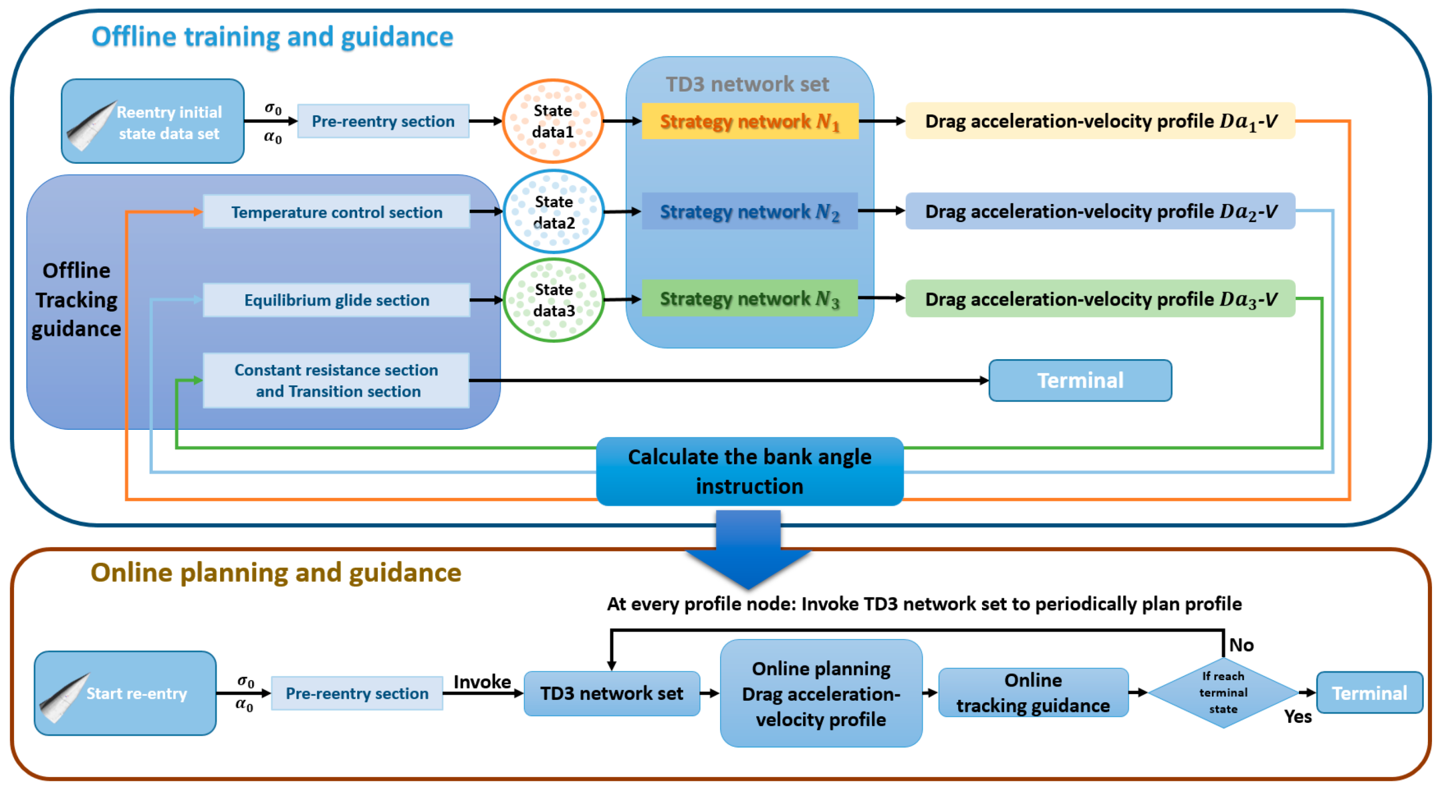
As shown in Figure 3, the online planning and guidance algorithm of reentry trajectory based on TD3 is divided into two parts: ① Offline training part—training multiple strategy networks by using TD3 algorithm framework by pulling off the initial states and tracking guidance offline; ② Online planning and guidance part—online invoke TD3 strategy network to plan and periodically update the drag acceleration profile, and the tracking guidance law is calculated online.

4.1. Offline Network Training Based on TD3

4.1.1. Twin Delayed Deep Deterministic Policy Gradient (TD3)

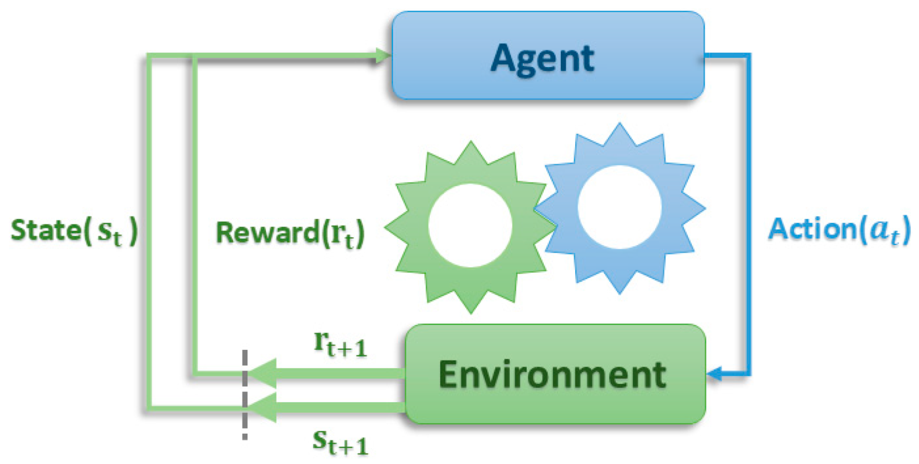
Reinforcement learning [19] belongs to the machine learning paradigm under the sequential decision-making framework. As shown in Figure 4, its core mechanism is reflected in the multi-step interaction process between the agent and the environment, imitating ‘trial and error learning’ of the organism mechanism so that an agent learns how to make a series of actions (Action) to change the state of the environment (State) to achieve the goal of maximizing the cumulative reward (Reward), and gradually approaching the optimal behavior strategy.

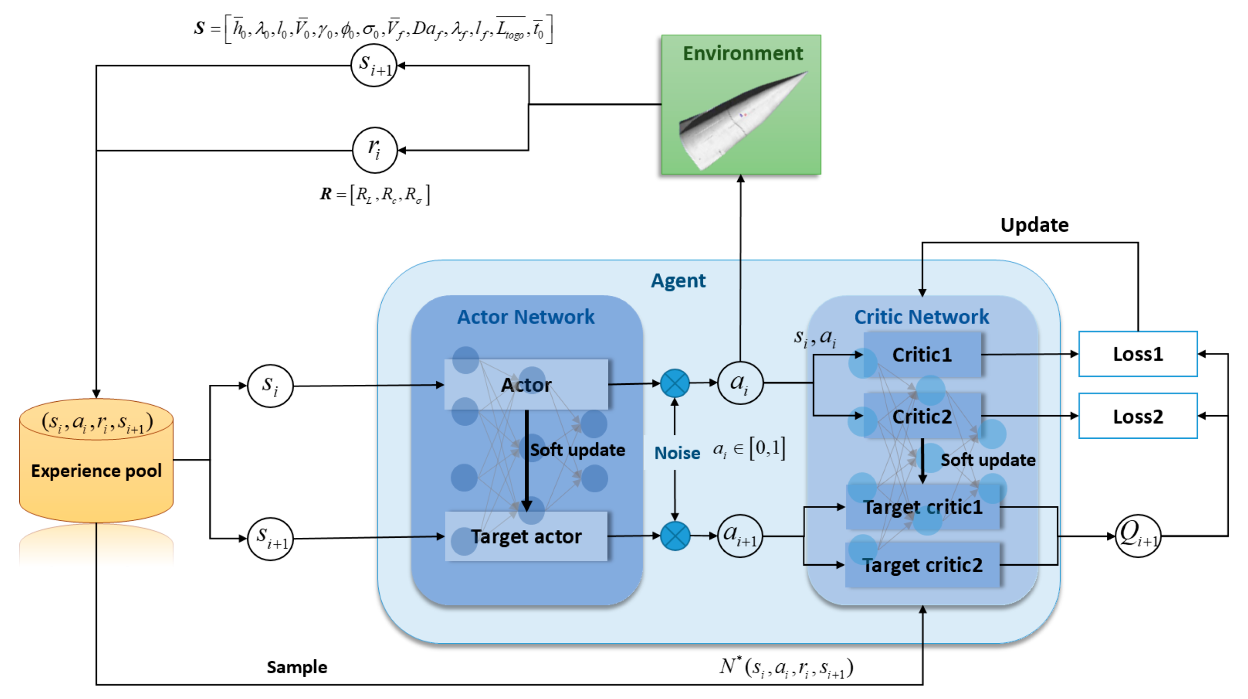
The TD3 [20] algorithm is a deep reinforcement learning algorithm based on the Actor–Critic framework, which aims to solve the problem of overestimation of Q value in deep deterministic policy gradient methods (such as deep deterministic policy gradient, DDPG). Its core design includes three key technologies: Clipped Double Q-Learning, Target Policy Smoothing, and Delayed Policy Updates.

• Clipped Double Q-Learning

In order to suppress the overestimation bias of the Q function, TD3 maintains two independent Critic networks $(Q_{{\theta }_1},Q_{{\theta }_2})$ and their target networks $(Q_{{\theta }_1^{’}},Q_{{\theta }_2^{’}})$ at the same time. The target Q value is generated by the minimum value of the two:

$$y=r_a+{\gamma }_a\min Q_{{\theta }_1^{’}}(s^{’},a^{’})$$

(25)

where $r_a$ is a reward signal caused by an action, ${\gamma }_a$ is the discount factor, and $(s^{’},a^{’})$ are the state and action of the next moment.

2.

Target Policy Smoothing

When TD3 calculates the target Q value, a small Gaussian noise is added to the target action to constrain the action disturbance range ($\left|\epsilon \right|\le c$) so that the Q function is locally smooth in the action space, avoiding the strategy overfitting to the sharp peak of the Q function.

$$a^{’}={\pi }_{{\varphi }^{’}}(s^{’})+\chi ,\chi ~clip(N(0,\sigma ),-c,c)$$

(26)

where $\chi$ is the random noise of a normal distribution, with the range being $\left(-c,c\right)$.

3.

Delayed Policy Updates

TD3 introduces a delay effect in the update mechanism of the Actor network; that is, the update of the Actor network will lag behind the multiple iterations of the Critic network, ensuring that the Actor can receive more stable and accurate Q value information.

4.1.2. TD3 Strategy Network Designing

Considering the environmental uncertainty and the bank angle reversal strategy adopted by the lateral guidance, there is a limit on the amplitude of the change rate when the bank angle is reversed, and the reversal is not completed instantaneously. It is necessary to consider the time required for the roll angle reversal during the actual flight process, resulting in insufficient accuracy of the final landing point of the aircraft. In order to improve this shortcoming, the core idea of the TD3 trajectory online planning algorithm is to train three different TD3 reinforcement learning strategy networks $N_i$($i=1,2,3$): ① Strategy network $N_1$: The initial states of reentry are biased, the terminal state data set of the pre-reentry section is collected offline, and the strategy network $N_1$ is trained to generate the drag acceleration profile of the whole section of the gliding section at the beginning of the gliding section. ② Strategy network $N_2$: The tracking guidance is carried out offline for the drag acceleration profile of the temperature control section. The terminal state data set of the temperature control section is collected offline, and the training strategy network $N_2$ is used to generate the drag acceleration profile of the equilibrium glide section, the constant drag section and the transition section at the beginning of the equilibrium glide section. ③ Strategy network $N_3$: The tracking guidance is carried out offline for the drag acceleration profile of the balanced glide section. The terminal state data set of the balanced glide section is collected offline, and the training strategy network $N_3$ is used to generate the drag acceleration profile of the constant resistance section and the transition section at the beginning of the constant resistance section. By invoking the TD3 strategy network $N_i$ planning trajectory multiple times online at each node of the glide section, it is combined with the tracking guidance so that the cumulative error in the previous guidance period can be eliminated each time the algorithm is invoked again, and the accuracy of the aircraft landing point can be improved.

TD3 strategy network training needs to set up three parts, namely state space (State), action space (Action), and reward (Reward).

• State space

The state vector $S\in {\mathit{R}}^{13}$ comprehensively characterizes the initial motion state and task target of the aircraft.

$$\mathit{S}=\left[{\overline{h}}_0,{\lambda }_0,l_0,{\overline{V}}_0,{\gamma }_0,{\varphi }_0,{\sigma }_0,{\overline{V}}_f,D{a}_f,{\lambda }_f,l_f,\overline{L_{togo}},{\overline{t}}_0\right]$$

(27)

where ${\overline{h}}_0$, ${\overline{V}}_0$, $\overline{V_f}$, $\overline{L_{togo}}$, and ${\overline{t}}_0$ are the normalized initial height and velocity, terminal velocity, distance, and time between the aircraft and the endpoint, respectively.

The first seven states reflect the initial motion state of the aircraft, the eighth to eleventh states give the task target information, and finally reflect the terminal waiting distance and simulation time. In order to eliminate the influence of dimension on training, some parameters of the state space are normalized. The normalization method is as follows:

$$\overline{x}={\displaystyle \frac{x}{k}}$$

(28)

where $\overline{x}$ is the normalized variable and $k$ is the normalized coefficient, see

Table 1. Normalized coefficient.

Variable	Unit	Coefficient
$h$	m	$R_{\mathrm{e}}$
$V$	m·s−1	$\sqrt{g_0{R}_{\mathrm{e}}}$
$L_{togo}$	m	$R_{\mathrm{e}}$
$t$	s	10

.

2.

Action space

By designing the action space, the drag acceleration profile parameters can be solved to determine the size and shape of the profile. According to the different trajectory generation tasks of three different strategy networks $N_i$, the action space $\mathit{A}$ to be designed is different. Therefore, each action output by the agent is normalized as $a_i\in \left[0, 1\right]$, and the specific design is as follows:

• Strategy network $N_1$:

$$\mathit{A}=[a_1,a_2,a_3]$$

(29)

$$\left\{\begin{array}{l}{V}_1=V^{Qm}+a_1\ast (V^{Qn}-V^{Qm})\\ V_2=V_{alpha\downarrow }+a_2\ast (V_1-\delta -V_{alpha\downarrow })\\ V_3=V_z+\epsilon +a_3\ast (V_2-V_z-\epsilon )\end{array}\right.$$

(30)

• Strategy network $N_2$:

$$\mathit{A}=[a_2,a_3]$$

(31)

$$\left\{\begin{array}{l}{V}_2=V_{alpha\downarrow }+a_2\ast (V_1-\delta -V_{alpha\downarrow })\\ V_3=V_z+\epsilon +a_3\ast (V_2-V_z-\epsilon )\end{array}\right.$$

(32)

• Strategy network $N_3$:

$$\mathit{A}=a_3$$

(33)

$$V_3=V_z+\epsilon +a_3\ast (V_2-V_z-\epsilon )$$

(34)

3.

Reward

The reward function in reinforcement learning is the core of driving agent learning, and its design quality directly determines the success or failure of reinforcement learning training. In this paper, a hierarchical reward design method is adopted to meet the requirements of the flight range under the condition of satisfying the process constraints so that the aircraft can successfully reach the target point.

• Flight distance reward $R_L$

The goal of the reward is to guide the aircraft to gradually approach the target point, and the reward is negatively correlated with the terminal flight range. Therefore, a piecewise linear function reward is designed to make the terminal flight range smaller and the reward greater.

$$R_L=\left\{\begin{array}{cc}{r}_1\ast (L_1-L_{\mathrm{togo}})& L_{\mathrm{togo}}<L_{goal1}\\ r_2\ast (L_2-L_{\mathrm{togo}})+r_1\ast (L_1-L_{goal1})& L_{goal1}\le L_{\mathrm{togo}}<L_{goal2}\\ r_2\ast (L_2-L_{goal2})& L_{\mathrm{togo}}\ge L_{goal2}\end{array}\right.$$

(35)

where $r_1$, $r_2$, $L_1$, $L_2$, $L_{goal1}$, and $L_{goal2}$ are all positive coefficients.

• Process constraint reward $R_c$

The drag acceleration profile exceeds the reentry corridor and is given a negative reward. If it does not exceed, no reward is given.

$$R_c=\left\{\begin{array}{ll}-a_c& Da\le D{a}_{down}\\ -a_c& D{a}_{up}\le Da \\ 0& D{a}_{down}<Da<D{a}_{up}\end{array}\right.$$

(36)

where $a_c$ is a positive coefficient.

• Bank angle reversal reward

In order to reduce the inclination angle reversal, when the total number of inclination angle reversals exceeds a certain value, a negative reward is given.

$$R_{\sigma }=\left\{\begin{array}{ll}-a_{\sigma }& T(\sigma )>T{(\sigma )}_{\max }\\ 0& else\end{array}\right.$$

(37)

where $a_{\sigma }$ is a positive coefficient, $T(\sigma )$ is the number of bank angle reversals in the whole reentry process of the aircraft, and $T{(\sigma )}_{\max }$ is limitation of the number of bank angle reversals.

In summary, the sum of the aircraft final awards is

$$R=R_L+R_c+R_{\sigma } \mathrm{IsDone}$$

(38)

where $\mathrm{IsDone}=\sqrt{{(V-V_f)}^2}\le \Delta V$ represents the end of the training round and $\Delta V$ is the terminal velocity threshold.

The TD3 strategy network design logic is the state quantity of the aircraft as the environmental state, and the agent uses a dual Critic network and a delay strategy to update the collaborative optimization. By updating the two Critic networks in parallel and taking the minimum value to construct the target Q value to suppress the overestimation bias, the Actor network is gradually optimized at a lower update frequency than the Critic network to ensure the stability of the function evaluation. At the same time, the clipping Gaussian noise is added to the output action of the target Actor to smooth the Q value estimation surface, and the soft update mechanism is used to gradually synchronize the target network parameters, and finally, output the action to maximize the reward, as shown in Figure 5.

4.2. The Tracking Guidance

4.2.1. Longitudinal Guidance

In the TD3 trajectory online planning algorithm, the drag acceleration–velocity profile solved by the strategy network can be converted into a height–velocity profile. Combined with the 3-DOF reentry dynamic model, the amplitude of the bank angle can be inversely solved.

Through the transformation of Equation (1), it can be obtained that

$${\displaystyle \frac{dH}{dV}}={\displaystyle \frac{V\sin \gamma }{-\frac{D}{m}-g\sin \gamma +{\tilde{C}}_V}}$$

(39)

When the height–velocity profile is known, the height can be expressed as a function related to the velocity, and the corresponding velocity derivative ${\displaystyle \frac{dV}{dH}}$ can be obtained by the difference in the velocity. Given the size of the track angle, the difference method is used again to obtain the corresponding velocity derivative ${\displaystyle \frac{d\gamma }{dV}}$, and according to the chain derivative rule, the change rate of the track angle can be obtained, that is,

$${\displaystyle \frac{d\gamma }{dt}}={\displaystyle \frac{d\gamma }{dV}}\ast {\displaystyle \frac{dV}{dt}}={\displaystyle \frac{d\gamma }{dV}}\ast (-{\displaystyle \frac{D}{m}}-g\sin \gamma +{\tilde{C}}_V)$$

(40)

The change rate of the track angle is known, and the size of the bank angle can be expressed as

$$\sigma =acr\cos ({\displaystyle \frac{V(\stackrel{·}{\gamma }-{\tilde{C}}_{\gamma })-(V^2/r-g)\cos \gamma }{L/m}})$$

(41)

The longitudinal guidance directly tracks the bank angle without correction.

4.2.2. Lateral Guidance

Because the angle of attack profile is preset, the lateral guidance only needs to determine the sign of the bank angle, and the change process of the remaining state quantity can be obtained by numerical integration of the dynamic equations of longitude, latitude, and heading angle.

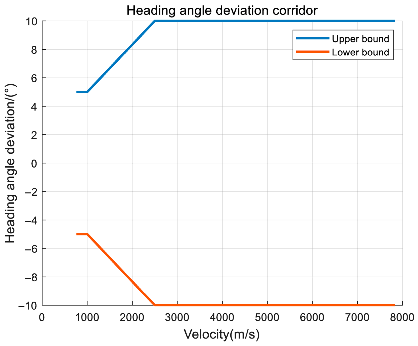
In this paper, the sign of the bank angle is obtained by using the bank angle reversal control strategy. The basic idea can be described as follows: by giving the heading angle deviation corridor, when the velocity heading angle of the aircraft exceeds the maximum range allowed by the corridor, the aircraft immediately reverses the bank angle, that is, the sign of the bank angle so that the velocity heading angle returns to the established range to ensure that the spacecraft flies towards the target point, which is expressed by the followingformula:

$$\mathrm{sgn}\left({\sigma }^{(t)}\right)=\left\{\begin{array}{cc}-1& \Delta \varphi \ge \Delta {\varphi }_{\mathrm{up}}\\ \mathrm{sgn}\left({\sigma }^{(t-1)}\right)& \Delta {\varphi }_{\mathrm{down}}<\Delta \varphi <\Delta {\varphi }_{\mathrm{up}}\\ 1& \Delta \varphi \le \Delta {\varphi }_{\mathrm{down}}\end{array}\right.$$

(42)

where $\Delta {\varphi }_{\mathrm{up}}$ and $\Delta {\varphi }_{\mathrm{down}}$ are the designed corridor boundaries, and

$$\begin{array}{l}\Delta {\varphi }_{\mathrm{up}}=\left\{\begin{array}{cc}{\varphi }_1& V\ge V_m\\ {\varphi }_1-{\displaystyle \frac{V-V_1}{V_2-V_1}}{\varphi }_2& V_m>V>V_n\\ {\varphi }_2& V<V_n\end{array}\right.\\ \Delta {\varphi }_{\mathrm{down}}=-\Delta {\varphi }_{\mathrm{up}}\end{array}$$

(43)

where $V_m$, $V_n$, ${\varphi }_1$, and ${\varphi }_2$ are the velocity heading angle deviation corridor parameters designed according to experience.

When the velocity of the aircraft is high, the distance between the aircraft and the target point is far, and there is more time to adjust the error, so a larger heading angle error corridor is set to reduce the number of roll angle reversals. When approaching the target point, in order to improve the terminal accuracy, it is necessary to narrow the range of the heading angle error corridor, as shown in the following Figure 6.

4.3. Online Trajectory Planning and Guidance

Combined with the TD3 strategy network set of offline training, online trajectory generation and guidance can be realized, as shown in Figure 3. The initial state of the aircraft is determined, and the aircraft maintains a constant bank angle and angle of attack to complete the pre-reentry section flight. The TD3 strategy network $N_1$ is invoked at the end node of the pre-reentry section to generate the entire drag acceleration profile of the glide section online for online tracking guidance. The TD3 strategy network $N_2$ is invoked at the end node of the temperature control section to generate the drag acceleration profile of the equilibrium glide section, the constant resistance section, and the transition section online for online tracking guidance. The TD3 strategy network $N_3$ is invoked at the end node of the equilibrium glide section to generate the drag acceleration profile of the constant resistance section and the transition section online for online tracking guidance, thereby completing the flight task. The TD3 strategy networks are trained offline and invoked online many times so that the cumulative error in the previous guidance period can be eliminated when the algorithm is called again each time, and the online rapid generation and update of the reentry trajectory is realized, which effectively improves the accuracy and computational efficiency of the landing point. Due to the black box characteristics of the trained neural network, it is difficult to absolutely guarantee the reliability of the algorithm. In actual execution, in order to avoid security risks, the complete or stage trajectory can be quickly integrated to evaluate the reliability of the trajectory. On the other hand, the TD3 guidance strategy does not exclude the involvement of other algorithms. For example, traditional guidance methods such as predictive correction guidance can be used to take over for a short time.

5. Simulation and Discussion

• TD3 strategy network offline training

According to the above settings, the training agent is trained. The initial state of training is set as shown in

Table 2. Initial state of training.

Parameter	Unit	Pull Deviation Situation
$H$	m	$\pm 2000$
$V$	m·s−1	$\pm 10$
$\gamma$	°	$\pm 0.5$
$\lambda$	°	$\pm 1$
$l$	°	$\pm 1$
$\varphi$	°	$\pm 3$

, and the initial state is uncertainly biased.

The TD3 strategy network training results are compared with the DDPG training results to verify that the TD3 online trajectory planning algorithm has strong adaptability and robustness. Firstly, the training network parameters of TD3 and DDPG are set: ① TD3 network module: The Actor network and Critic network modules have two hidden layers, and the two hidden layers contain 1024 and 512 neurons, respectively; the learning rates of the Actor network and Critic network are 0.0001 and 0.0001, respectively; the size of the playback buffer is ${10}^6$; the sampling batch size of each training is 256; the discount factor is 0.99; the soft update coefficient of the target network is 0.005; and the target strategy Gaussian noise is $(-0.5, 0.5)$. ② DDPG network module: The Actor network module and Critic network module have two hidden layers, and the two hidden layers contain 1024 and 512 neurons, respectively. The learning rates of the Actor network and Critic network are 0.001 and 0.001, respectively; the size of the playback buffer is ${10}^6$; the sampling batch size of each training is 256; the discount factor is 0.99; the soft update coefficient of the target network is 0.005; and the regression coefficient and variance of OU noise are 1 and 0.1, respectively. Secondly, the training process reward parameters are set. If the process constraint reward parameter is too large, the accuracy of the landing point will be affected. If the process constraint reward parameter is too small, the process constraint will not be satisfied. When setting the tilt angle reversal reward, if the number of bank angle reversal restrictions is too large or too small, the reward will be ineffective. If the tilt angle reversal reward is too large, it will affect the accuracy of the landing point. If it is too small, the reward will not work. It is necessary to train and debug multiple times to obtain the optimal result, as shown in

Table 3. Training process reward parameters.

Parameter	Value
$r_1$	24
$r_2$	12.67
$L_1$	5
$L_2$	3
$L_{goal1}$	5
$L_{goal2}$	13
$a_c$	20
$a_{\sigma }$	10
$T{(\sigma )}_{\max }$	5

.

Figure 7 shows the average reward variation curve of the training process. As shown in Figure 7 and

Table 4. Average reward convergence of strategy networks.

Network	DDPG	TD3
$N_1$	23	71
$N_2$	61	77
$N_3$	66	85

, during the whole training process, the average training reward of TD3 is much better than that of DDPG, which represents that the trajectory online generation and guidance algorithm based on TD3 reinforcement learning has strong applicability and robustness, and can adapt to different initial states and significant model parameters. And the convergence speed of TD3 is basically faster than DDPG. The average rewards of the three TD3 strategy networks are gradually increasing. When the training times are set to 1000 times, the rewards are gradually converged after training 600 rounds, indicating that the basic training of the TD3 strategy network is completed.

As shown in Table 4, whether TD3 or DDPG is used, the relationship between the convergence average reward values of the three strategy networks is $N_3>N_2>N_1$, which proves that the aircraft can improve the landing accuracy of the aircraft by calling the corresponding strategy network during the reentry process.

2.

Online trajectory planning and guidance

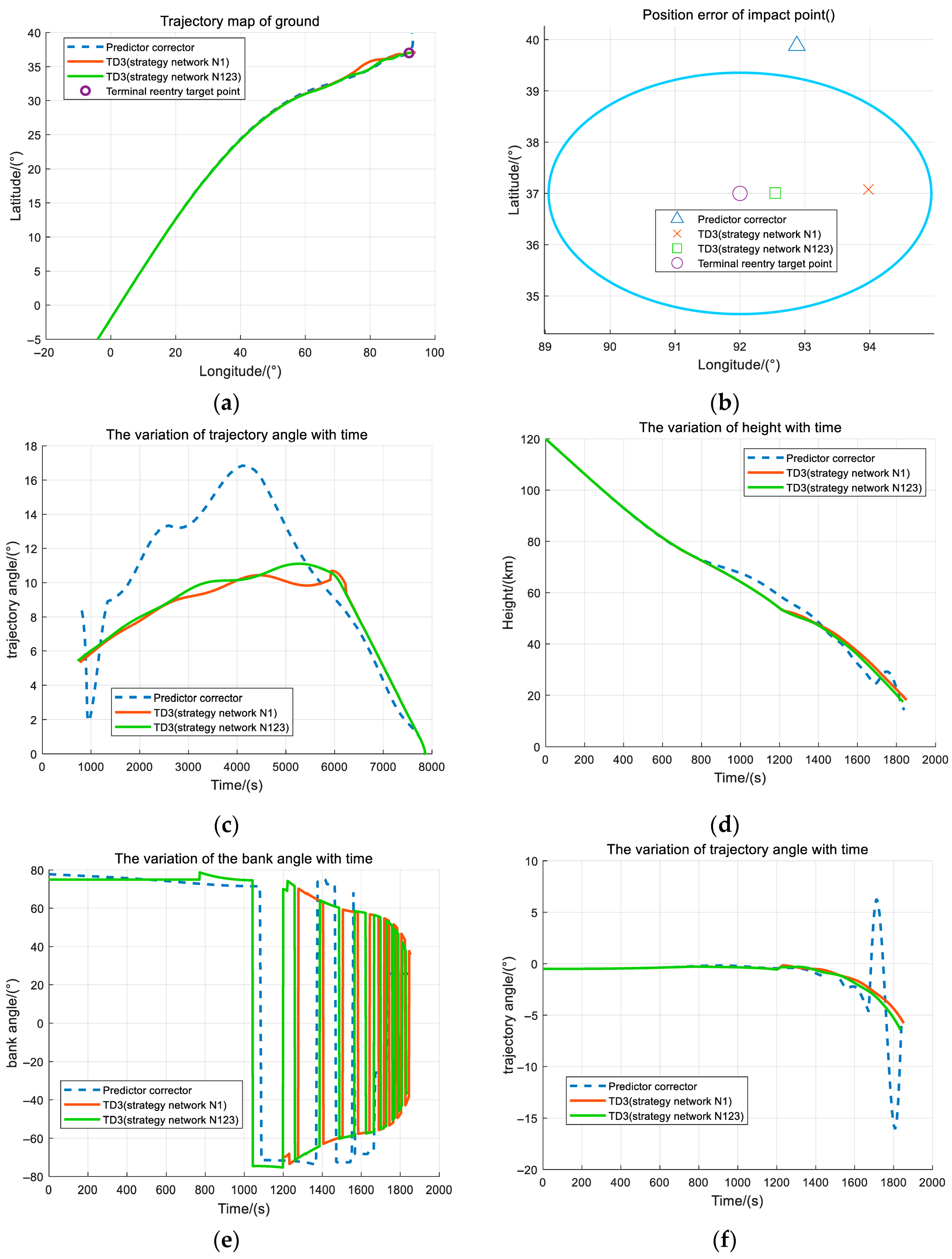
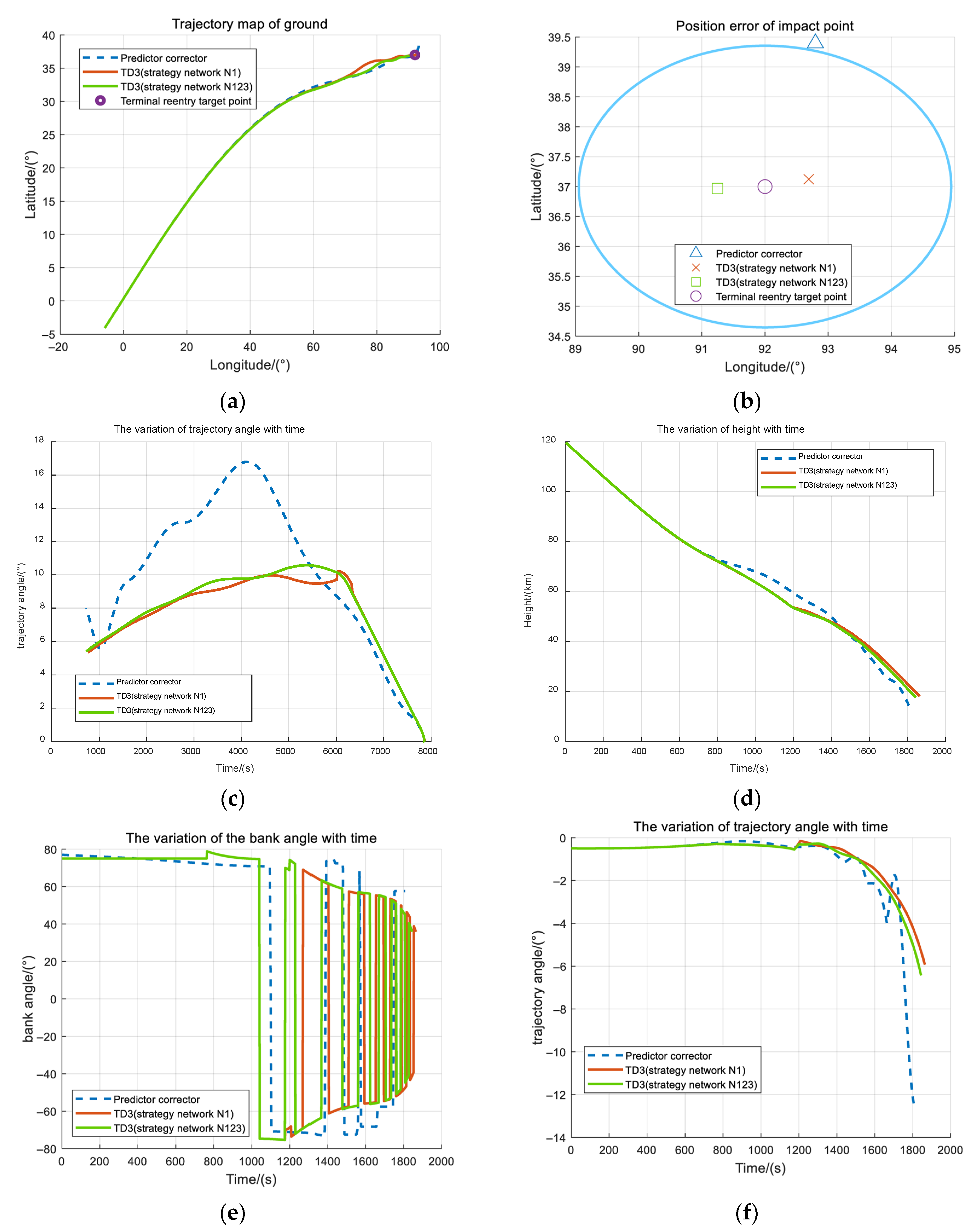
The initial state of the aircraft is given randomly, and determination of the aerodynamic uncertainty deviation is carried out. The specific guidance tasks and aerodynamic uncertainty are shown in

Table 5. Guidance tasks.

Task	Unit	1	2	3
$H$	km	119.947	119.878	118.609
$V$	m·s−1	7837.578	7834.569	7829.437
$\gamma$	°	0.678	0.795	0.834
$\lambda$	°	−5	−5.972	−4.068
$l$	°	−4.068	−5.316	−5.891
$\varphi$	°	53.453	54.754	53.167
$H_f$	km	18
$V_f$	m·s−1	760
${\lambda }_f$	°	37
$l_f$	°	92

and

Table 6. Aerodynamic uncertainty of aircraft.

Section	${\mathit{C}}_{\mathit{L}}$	${\mathit{C}}_{\mathit{D}}$
Equilibrium glide section	$+5\%$	$+5\%$

. The trajectory generation and guidance of the three tasks are carried out online, respectively. The simulation diagram is shown in Figure 8, Figure 9 and Figure 10.

In Figure 8a,b, Figure 9a,b and Figure 10a,b, it can be seen that in each task, the trajectory online generation and guidance algorithm based on TD3 reinforcement learning can complete the flight task; and the landing accuracy of the method of invoking the TD3 policy network multiple times is better than that of invoking a single policy network only in the pre-reentry section, and the two methods are better than the prediction–correction guidance. Figure 8c, Figure 9c and Figure 10c, show the drag acceleration profiles corresponding to the three tasks during the flight, and it can be seen that the algorithm can adapt to the requirements of the three tasks. In Figure 8d–f, Figure 9d–f and Figure 10d–f, it can be seen that the drag acceleration profile in the form of four multiple functions is used to make the trajectory angle not jump, so as to ensure that the aircraft can track the nominal trajectory during the guidance process, so that the aircraft can reach the terminal height and velocity.

Table 7. Simulation time.

Method	Unit	Average Total Time	Average Single Instruction Generation Time
Predictor-corrector	s	811.9202	0.5635
$\mathrm{TD}3 (\mathrm{strategy} \mathrm{network} N_1$)	s	3.5115	0.0039
$\mathrm{TD}3 (\mathrm{strategy} \mathrm{network} N_{1,2,3}$)	s	8.2866	0.0037

shows the simulation time of the three methods. The single command generation efficiency of the TD3 guidance method is improved by ${10}^2$, and the average single command generation is less than 0.01 s, which can realize real-time online guidance.

In summary, the most significant advantages of TD3-based reentry trajectory online planning and guidance compared to traditional guidance methods are as follows:

• Improve the accuracy of landing point: In the case that the traditional guidance method can also reach the target point, the TD3 guidance method has higher landing point accuracy, strong random error applicability, and flight adaptability, and the accuracy of the preset task is improved by 84%.
• The computational efficiency is improved: Compared with the traditional guidance method, the single command generation efficiency of the TD3 guidance method is improved by ${10}^2$, which can realize online guidance.
• Simplified longitudinal guidance strategy: Because the profile design of traditional drag acceleration–velocity profile guidance is not smooth, it is necessary to design the longitudinal guidance law offline to correct the bank angle, such as PID guidance. TD3 guidance smooths the angle of attack profile and the reference profile so that the calculated bank angle can be directly guided longitudinally to ensure that the aircraft tracks the nominal profile and achieves the effect of simplifying the guidance strategy.

6. Conclusions

Aiming at the problem of poor autonomy and weak time performance of reentry trajectory planning for RLV, an online reentry trajectory planning and guidance method based on TD3 reinforcement learning is proposed. The reference profile adopts four multi-function drag acceleration–velocity profiles designed in the reentry corridor to ensure smooth connection of turning points. The TD3 strategy networks are trained offline to solve the profile parameters to meet the needs of the flight range. According to the current state and flight range of each section of the drag acceleration profile, the TD3 strategy network is invoked multiple times online to plan the trajectory and update the profile periodically. The offline training and multiple online invoking of TD3 strategy networks can eliminate the cumulative error in the previous guidance cycle when the algorithm is invoked again each time, and the online rapid generation and update of the reentry trajectory is realized, which effectively improves the accuracy of the landing point and the efficiency of instruction generation, and provides an effective method for real-time online trajectory planning and autonomous guidance in the complex environment of aerospace vehicles.

References

1. Fan, W.; Wang, L.; Long, X.D. Review of Foreign Reusable Launch Vehicle Development in 2022. China Aerosp. 2023, 25–30. [Google Scholar]
2. Zhang, C.; Liu, D.Q.; Wang, J.W. Review of Foreign Hypersonic Technology Development in 2020. Aerosp. Missiles 2021, 12–16. [Google Scholar] [CrossRef]
3. Mu, L.X.; Wang, X.M.; Xie, R. Review of Hypersonic Vehicles and Their Guidance and Control Technologies. J. Harbin Inst. Technol. 2019, 51, 1–14. [Google Scholar]
4. Pan, L.; Peng, S.; Xie, Y. 3D Guidance for Hypersonic Reentry Gliders Based on Analytical Prediction. Acta Astronaut. 2020, 167, 42–51. [Google Scholar] [CrossRef]
5. Liu, Z.; He, Y. Study of Reentry Guidance Based on Analytical Predictor-Corrector for Aerospace Vehicle. In Proceedings of the 36th Chinese Control Conference, Dalian, China, 26–28 July 2017; pp. 5827–5832. [Google Scholar]
6. Yu, B. Research on Guidance Technology for Initial Reentry Phase of Reusable Launch Vehicle. Master’s Thesis, Nanjing University of Aeronautics and Astronautics, Nanjing, China, 2015. [Google Scholar]
7. Yu, L. Research on Guidance Technology for Reentry Phase of Reusable Launch Vehicle. Master’s Thesis, Nanjing University of Aeronautics and Astronautics, Nanjing, China, 2018. [Google Scholar]
8. Wang, P.; Yan, X.; Nan, W.; Li, X. A Rapid and Near Analytic Planning Method for Gliding Trajectory under Time Constraints. Acta Armamentarii 2024, 45, 2294–2305. [Google Scholar]
9. Wang, T.; Zhang, H.B.; Zhu, R.Y. Reentry Predictor-Corrector Guidance Algorithm Considering Drag Acceleration. J. Astronaut. 2017, 38, 143–151. [Google Scholar]
10. Huang, H.B.; Liang, L.Y.; Yang, Y. Reentry Trajectory Planning and Guidance Method Based on Inverse Drag Acceleration Profile. Acta Aeronaut. 2018, 39, 338–348. [Google Scholar]
11. Yan, X.L.; Wang, K.; Zhang, Z.J. Reentry Guidance Method Based on LSTM-DDPG. Syst. Eng. Electron. 2025, 47, 268–279. [Google Scholar]
12. Jiang, Q.; Wang, X.; Li, Y. Intelligent Reentry Guidance with Dynamic No-fly Zones Based On Deep Reinforcement Learning. In Proceedings of the 29th International Conference on Computational and Experimental Engineering and Science, Shenzhen, China, 3–6 August 2024; pp. 291–313. [Google Scholar]
13. Huang, X.Y.; Dai, J.; Liu, G. Predictor-Corrector Guidance Algorithm for Launch Vehicle Based on DDPG. Aerosp. Technol. 2024, 89–102. [Google Scholar]
14. Das, P.P.; Pei, W.; Niu, C. Reentry Trajectory Design of A Hypersonic Vehicle Based On Reinforcement Learning. In Proceedings of the 2023 Asian Aerospace and Astronautics Conference, Wuhan, China, 15–17 September 2023; p. 012005. [Google Scholar]
15. Hui, J.P.; Wang, R.; Guo, J.F. Intelligent Guidance Technology for No-Fly Zone Avoidance Based on Reinforcement Learning. Acta Aeronaut. 2023, 44, 240–252. [Google Scholar]
16. Hui, J.P.; Wang, R.; Yu, Q.D. Online Generation Technology of ‘New Quality’ Corridor for Reentry Vehicle Based on Reinforcement Learning. Acta Aeronaut. 2022, 43, 623–635. [Google Scholar]
17. Wang, Z.H.; Li, T.; Yan, H.D.; Hu, Y.; Gao, C. Improved Drag Acceleration Profile Design for Hypersonic Vehicle. Mod. Def. Technol. 2024, 52, 115–123. [Google Scholar]
18. Nie, Z.T. Reentry Trajectory Planning and Tracking Control Based on Altitude-Velocity Profile. Master’s Thesis, Dalian University of Technology, Dalian, China, 2020. [Google Scholar]
19. Barto, A.G.; Sutton, R.S. Reinforcement Learning: An Introduction; MIT Press: Cambridge, MA, USA, 1998. [Google Scholar]
20. Shi, L.A. Research on Deep Reinforcement Learning Methods and Applications. Master’s Thesis, Xidian University, Xian, China, 2023. [Google Scholar]
Figure 1. Angle of attack–velocity profile.
Aerospace 12 00747 g001
Figure 2. Drag acceleration–velocity corridor: (a) the reentry corridor boundary corresponding to each constraint; (b) reentry corridor composed of soft and hard constraints.
Aerospace 12 00747 g002
Figure 3. Algorithm structure diagram.
Aerospace 12 00747 g003
Figure 4. Reinforcement learning diagram.
Aerospace 12 00747 g004
Figure 5. Framework of designing TD3 strategy networks.
Aerospace 12 00747 g005
Figure 6. Heading angle deviation corridor.
Aerospace 12 00747 g006
Figure 7. Reward curves of training: (a) the reward convergences of TD3 and DDPG strategy network N 1 ; (b) the reward convergences of TD3 and DDPG strategy network N 2 ; (c) the reward convergences of TD3 and DDPG strategy network N 3 .
Aerospace 12 00747 g007aAerospace 12 00747 g007b
Figure 8. Simulation of task 1: (a) trajectory map of ground; (b) position error of impact point; (c) the variation in drag acceleration with velocity; (d) the variation in height with time; (e) the variation in the bank angle with time; (f) the variation in trajectory angle with time.
Aerospace 12 00747 g008
Figure 9. Simulation of task 2: (a) trajectory map of ground; (b) position error of impact point; (c) the variation in drag acceleration with velocity; (d) the variation in height with time; (e) the variation in the bank angle with time; (f) the variation in trajectory angle with time.
Aerospace 12 00747 g009
Figure 10. Simulation of task 3: (a) trajectory map of ground; (b) position error of impact point; (c) the variation in drag acceleration with velocity; (d) the variation in height with time; (e) the variation in the bank angle with time; (f) the variation in trajectory angle with time.
Aerospace 12 00747 g010