Article

Parameter Tuning of Detached Eddy Simulation Using Data Assimilation for Enhancing the Simulation Accuracy of Large-Scale Separated Flow Around a Cylinder

by
Kyosuke Nomoto
1,2,* and
Shigeru Obayashi
2
1
Department of Aerospace Engineering, Tohoku University, Sendai 980-8577, Miyagi, Japan
2
Institute of Fluid Science, Tohoku University, Sendai 980-8577, Miyagi, Japan
*
Author to whom correspondence should be addressed.
Aerospace 2025, 12(8), 736; https://doi.org/10.3390/aerospace12080736
Submission received: 30 December 2024 / Revised: 31 July 2025 / Accepted: 12 August 2025 / Published: 19 August 2025
(This article belongs to the Special Issue Fluid Flow Mechanics (4th Edition))

Abstract

In this study, data assimilation using PIV measurement data of the cylinder wake obtained from wind tunnel tests was applied to tune the simulation model parameters of Detached Eddy Simulation (DES) to improve the accuracy of large-scale separated flow simulations around a cylinder. The use of DES enables more accurate simulation of large-scale separation flows than RANS. However, it increases computational costs and makes parameter tuning using data assimilation difficult. To reduce the computational time required for data assimilation, the conventional data assimilation method was modified. The background values used for data assimilation were constructed by extracting only velocity data from locations corresponding to observation points. This approach reduced the computational time for background error covariance and Kalman gain, thereby significantly reducing the execution time of the filtering step in data assimilation. As a result of tuning, C d e s significantly increased, while C b 1 decreased. This adjustment extended the length of the recirculation bubble, bringing the time-averaged velocity distribution closer to the PIV measurement data. However, the peak frequency in the PSD obtained from the FFT analysis of velocity fluctuations in the wake shifted slightly toward lower frequencies, slightly increasing the discrepancy with the measurement data. Verifying the relationship between parameter values and flow, it was found that parameter tuning stabilized the separation shear layer generated at the leading edge of the cylinder and enlarged the size of the recirculation bubbles. On the other hand, frequency variations did not show consistent changes in response to parameter value changes, indicating that the effect of parameter tuning was limited under the simulation conditions of this study. To bring the frequency fluctuations closer to experimental results, it is suggested that other methods, such as higher-order spatial and temporal accuracy, should be combined.

1. Introduction

Computational Fluid Dynamics (CFD) has become increasingly valuable for analyzing fluid motion due to advancements in computational accuracy. Recently, high-fidelity simulations, such as Direct Numerical Simulation (DNS) and Large Eddy Simulation (LES), have become feasible. However, these methods require large amount of computational resources. Therefore, without a High Performance Computing (HPC) system, it is challenging to apply these methods in aerospace engineering and complex flow conditions, such as those involving aircraft and spacecraft. In fact, research analyzing the flow around wing profiles at high Reynolds numbers similar to flight conditions using LES used the one of the most powerful HPC in the world at the time of the study [1]. Even if computing performance continues to improve in the future, it is considered difficult to easily perform simulations that require such enormous computing resources.
Practically, simulations based on Reynolds-averaged Navier-Stokes equations (RANS) are commonly performed. However, these methods approximate turbulent behavior through mathematical models, resulting in high model dependence. In addition, turbulence models have difficulty accurately representing the complex motion of turbulence, making it difficult to perform highly accurate simulations under conditions where the spatio-temporal behavior of turbulence structures governs the flow. Consequently, RANS-based turbulent simulations have low accuracy in several cases, especially in conditions involving large scale separation flow such as the flow around a wing section with a high angle of attack [2,3]
To efficiently simulate the turbulent flow with large scale separation, hybrid simulations combining RANS and LES, such as Detached Eddy Simulation (DES) [4], have been proposed. DES applies the RANS method for flows near the solid body surface and the LES method for flows far from the solid body surface. The method explicitly decomposes lattice-scale vortices, resulting in higher reproducibility of turbulent structures than RANS, and allows for coarser grid spacing near object surfaces than LES, resulting in lower computational costs. So, it has been used industrially, including simulations of the flow around a landing gear [5] and a reentry capsule [6]. Nevertheless, DES results depend on grid size and turbulence model parameters [7]. Therefore, DES is not yet an ideal simulation method capable of accurately simulating all flow conditions. Modified methods have been proposed to improve computational accuracy by adjusting the switching region between RANS and LES, similar to Delayed DES (DDES) [8] and Improved DDES (IDDES) [9], but these methods were not sufficient to completely resolve the accuracy issues.
Recently, data assimilation method, which tunes turbulence model parameters using experimental or observation data, has attracted attention as a means to improve simulation accuracy by adjusting the simulation method to the real flow phenomena. Data assimilation incorporates “observation data” which is obtained experiment into numerical simulations, a method extensively developed in weather forecasting. Several studies applying this method to RANS simulations have demonstrated improved accuracy. For example, a study tuned the parameters of the Menter SST model using wind tunnel velocity data for back-step flow [10], and another study adjusted the parameters of the k ϵ model using LES data on surface pressure distribution for flow around a square cylinder [11].
In this study, similarly to previous RANS-focused research, we attempted to enhance simulation accuracy by tuning DES model parameters through data assimilation using experimental data. We examined the flow around a circular cylinder with low aspect ratio levitated in the freestream, a type of large-scale separated flow, which is an important flow condition in aerodynamic engineering. The flow is characterized by a separated shear layer at the leading edge of the cylinder, and a turbulent structure forming at the cylinder wake called the “recirculation bubble” and the “helical vortex structure” [12].
Large-scale separation flow is observed in aircraft stall conditions and around spacecraft, and they significantly affect the stability, so its phenomenon must be simulated with high accuracy. In several studies, to precisely represent this phenomenon in numerical simulation, a high-fidelity and high-cost simulation method such as LES or DNS is required [13,14,15]. In addition, wind tunnel tests can provide high-fidelity flow data by replicating actual flow conditions as closely as possible. However, location, quantity, and types of physical quantities of data that can be obtained are constrained by the specifications of the experimental apparatus and experimental methods, and there are cases where it is not possible to obtain all the necessary data. Furthermore, studies on improving the simulation accuracy of flows accompanied by separation through RANS parameter tuning have achieved qualitative improvements in accuracy but have not been able to reproduce observation data [11,16]. This study aims to reproduce airflow similar to wind tunnel test using DES with low computational costs through parameter tuning using data assimilation. This is expected to not only improve simulation accuracy but also realize an alternative to wind tunnel experiments, thereby contributing to the advancement of research and development in aerospace engineering.
The observation data used for data assimilation were two-dimensional velocity distributions measured using Particle Image Velocimetry (PIV) in the back of a circular cylinder levitated in freestream by Magnetic Suspended and Balance System (MSBS) [17]. The experiment was implemented by Kuwata et al. [18]. Conventional data assimilation methods required a significant amount of time and memory for matrix calculations, resulting in high computational costs. To address this issue, we extracted only the velocity data corresponding to the observation data acquisition locations from the simulation results obtained using DES and used it for data assimilation, thereby reducing the data assimilation cost. Additionally, the causal relationship between parameter changes and simulation results was investigated, and the mechanism by which parameter adjustments influence simulation results was examined.
The structure of this paper is as follows: Section 1 provides an overview of the background and objectives of the study; Section 2 describes the DES model, data assimilation method, and simulation conditions; Section 3 presents the result of parameter tuning, turbulent viscosity, and comparisons between simulations and PIV measurements of Reynolds stress, time-averaged velocity, velocity frequency analysis, and vorticity; and also examines the mechanisms for improving simulation accuracy based on changes in simulation results due to parameter adjustments; and finally, Section 4 presents the conclusions.

2. Methodology

2.1. Simulation Models and Parameters

The DES employed in this study is a type known as Delayed Detached Eddy Simulation (DDES), which was proposed by Spalart et al. in 2006 [8]. This DES model utilizes a modified version of the Spalart-Allmaras model [19], known as SA-noft2, which omits the transition terms from the original formulation. The SA-noft2 model is used as the turbulence model in the RANS region as well as the SGS model in the LES region. The transport equation for the modified turbulent viscosity coefficient ν ^ used in SA-noft2 is presented below.
ρ ν ^ t + ρ u j ν ^ x j = ρ C b 1 S ^ ν ^ C w 1 f w ν ^ d 2 + ρ σ x j ( ν + ν ^ ) ν ^ x j + C b 2 ν ^ x i ν ^ x i
where the first term on the right side represents the production term of turbulent viscosity, the second term represents the destruction term, and the third term represents the diffusion term. In the DES framework using the SA model, the length scale d (the distance from the wall surface) in the destruction term of the SA model is modified as follows:
d ˜ = min ( d , C des Δ ) ,
where Δ is the grid size, and C d e s is an empirically determined parameter. With this modification, the SA model operates as a RANS model in the regions where d < C des Δ and as an SGS model for LES in the regions where d > C des Δ . In DDES, the function is further modified as follows:
d ˜ = d f d max ( 0 , d C des Δ ) ,
where f d is a shielding function designed to prevent premature switching from RANS to LES in the boundary layer.
Since these equations include several empirically determined parameters, we attempted to reproduce the flow observed in wind tunnel tests by tuning these parameters using data assimilation. While tuning a larger number of parameters increases the degrees of freedom, potentially allowing the simulation to better replicate the experimental flow, it also significantly increases the computational cost required for data assimilation. Therefore, in this study, we selected parameters that are expected to have a significant impact on the flow field and focused on tuning them to perform computationally efficient data assimilation.
The parameters selected for tuning are C d e s and C b 1 . The parameter C d e s in DES adjusts the transition distance from the wall between RANS and LES, as well as the vortex size treated as turbulent viscosity in the LES region. The parameter C b 1 appears in terms of turbulent viscosity production and destruction in the SA model and affects the rate of turbulent viscosity generation.

2.2. CFD Code and Simulation Conditions

The CFD solver “UTCart,” a compressible fluid solver utilizing hierarchical Cartesian grids, developed by Imamura and Tamaki et al. [20] UTCart automates the processes of fluid simulations such as grid generation, numerical simulation of fluid, and output of flow data.
However, because hierarchical Cartesian grids consist of cubic cells, an excessive number of grids tends to accumulate near the object surface. In standard fluid simulations, the grid spacing on the object surface is set to satisfy the non-dimensional length y + < 1.0 . If the same grid resolution is applied in this study, the total number of grid points would reach the order of 10 8 . To address this issue, the wall-function feature implemented in UTCart was used, allowing for coarser grid spacing near the wall surface, which controlled excessive grid generation around the cylinder.
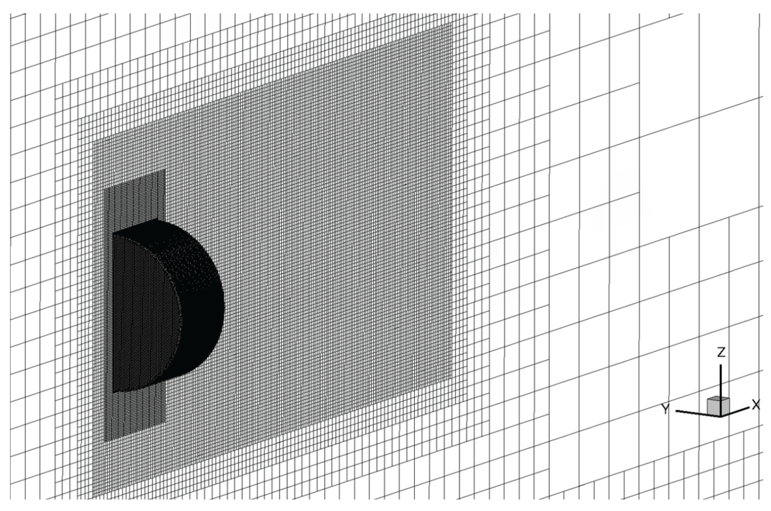
The cylinder size was set to match the cylinder used in the wind tunnel tests conducted by Kuwata et al. [18], with a diameter D = 1 , length L = 0.5 , and aspect ratio L / D = 0.5 (in the simulations, the length was non-dimensionalized by the diameter of the cylinder). The Reynolds number of the bulk flow was 5.9 × 10 4 , and the Mach number was set to 0.2. Figure 1 illustrates the computational domain and grid layout. To simulate flow conditions close to the wind tunnel tests, the external boundaries in the spanwise direction of the cylinder were set as slip wall boundaries to emulate the wind tunnel walls. The inlet boundary was set with total pressure and total temperature fixed to correspond to a Mach number of 0.2, while the outlet boundary was set as a fixed static pressure boundary. The cross-sectional width of the simulation domain was set to five times the diameter of the cylinder, matching the ratio of the diameter of the cylinder to the size of the wind tunnel used in the Kuwatas’ experiment [18]. In addition, initial flow condition was assumed to be uniform flow condition.
As shown in Figure 2, to visualize the recirculation bubble in the cylinder wake, the grid spacing in the wake region was set to D/45, so the total number of grid points is approximately 3.5 million. Although this resolution is appreciably coarse compared to LES simulations, we intentionally used such a coarse grid in this study to demonstrate the potential utility of improving simulation accuracy through parameter tuning via data assimilation under such conditions.
The computational methods used in the fluid simulations are as follows. Spatial gradients were computed using the weighted least squares method [21] and gradient reconstruction was performed using the second order MUSCL scheme [22]. Due to the low Mach number of 0.2 in this study, no slope limiting function was applied. The convection scheme used was SLAU, developed by Shima et al. [23], and the time integration method was LUSGS [24]. The time step was set to a non-dimensional time Δ t = 1.041666 × 10 2 , corresponding to 1 / 400 of the time step of the PIV measurement data ( 1 / 300 s) obtained in the wind tunnel tests.
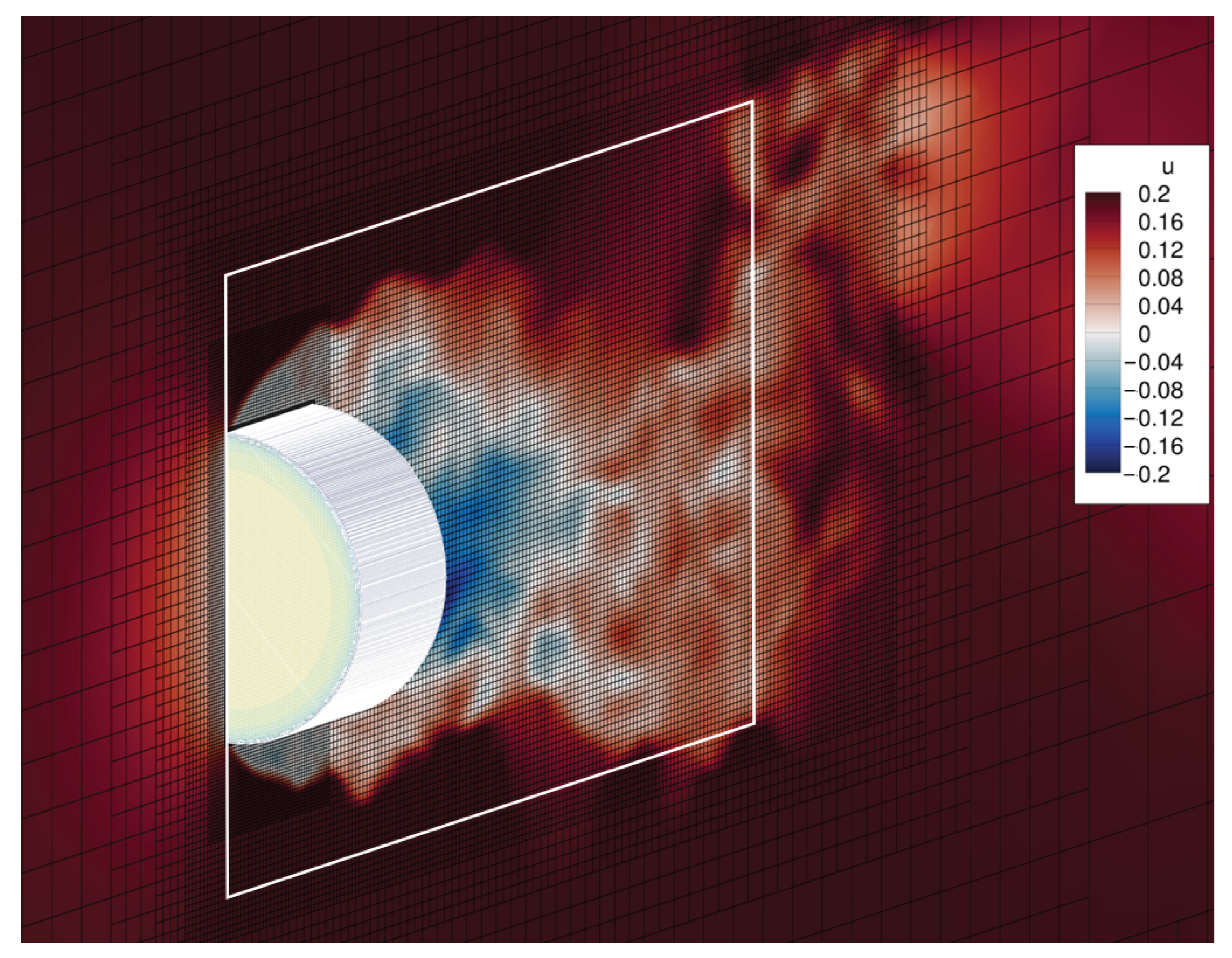
In the simulation, the flow separates at the leading edge of the cylinder, forming a large separation region in the cylinder wake. In this study, we evaluated the effect of parameter tuning on improving accuracy by comparing the velocity distribution in the x-z plane passing through the center axis of the cylinder (corresponding to the region where the PIV data were acquired) with the PIV measurement data, as shown in Figure 3.

2.3. Data Assimilation Method

Data assimilation methods can broadly be categorized into sequential data assimilation, based on Bayesian estimation theory, and variational data assimilation, based on the maximize the likelihood distribution. In this study, we used the “Ensemble Square Root Filter (EnSRF) [25],” a sequential data assimilation method. Since EnSRF is a variant of the Ensemble Kalman Filter (EnKF) [26], we first provide a brief overview of EnKF before explaining EnSRF. The data assimilation system can be represented by the following state-space model:
x t = F t x t 1 + v t
y t = H t x t + w t
where x t represents the state vector at time t, F t denotes the model operator that transitions the state from time t 1 to t, and v t is the system noise. Similarly, y t denotes the equivalent vector for the observation at time t, H t is the observation operator that maps the state to the observation space, and w t represents the observation error.
The EnKF performs data assimilation in a manner like the Kalman Filter (KF), which minimizes the error covariance of the simulation. The KF determines the correction weights using a function called the Kalman gain, as shown in Equation (6), and applies the correction to the state vector x t as expressed in Equation (7) and the simulation error covariance matrix V t as expressed in Equation (8).
K t = V t f H t T H t V t f H t T + R t 1
x t a = x t f + K t y t o b s H t x t f
V t a = I K t H t V t f
where K t is the Kalman gain, V t f is the simulation error covariance matrix, I is the identity matrix, H t is the observation operator, R t is the observation error covariance matrix, and the superscripts f and a represent ‘forecast’ and ‘analysis’, before and after data assimilation, respectively.
KF assumes linearity in both the system model and the observation model, making it unsuitable for direct application to fluid simulations, which are inherently non-linear systems. Furthermore, the covariance matrix V t is a matrix L × L , where L represents the number of elements in the state vector x t . In fluid simulations, L is often on the order of several millions, resulting in an overwhelming number of matrix elements. Consequently, the computational cost becomes prohibitively high, rendering such calculations practically infeasible.
The EnKF was proposed by Evensen to extend the KF framework for application to nonlinear models. This method approximates the error-containing state vector using a dataset of several state vectors, called an “ensemble,” which is constructed by introducing variability into the computational conditions.
X t f = x t f ( 1 ) x t f ( 2 ) x t f ( N )
where the superscripts ( 1 ) , ( 2 ) , , ( N ) denote the ensemble members. The mean and covariance of this ensemble are calculated using the following equations:
x t f ¯ = 1 N n = 1 N x t f ( n )
V t f = 1 N 1 n = 1 N x t f ( n ) x t f ¯ x t f ( n ) x t f ¯ T
In the EnKF, the ensemble covariance matrix is not explicitly updated because it is approximated by the update of each ensemble member. The Kalman Gain is derived using the above ensemble covariance matrix and the error covariance matrix of the observed data, and data assimilation is performed independently for each ensemble member using the Kalman Gain. Therefore, Equation (8) is skipped and data assimilation can be performed only by updating the state vector and Kalman Gain as shown below.
K t = V t f H t T H t V t f H t T + R t 1
x t a = x t f + K t y t o b s + w t n H t x t f
In the original EnKF process, as shown in the preceding equation, the observation vector y t o b s is added with different observation noise w t n for each ensemble member. This type of data assimilation process, in which observation noise is added to the observation data, is called the perturbed observation method, and the covariance matrix of the ensemble after data assimilation corresponds to the update formula of the covariance matrix of the KF. EnKF has proven great effectiveness by many researchers, but it also has shortcomings. One of them is that the noise added to the observation data when using the perturbed observation method causes sampling errors, which may impose a negative effect on the prediction of the state vector.
To avoid this issue, this study employed the Ensemble Square Root Filter (EnSRF), which does not require explicit addition of observation noise. In this method, similar to the Kalman Filter (KF), the ensemble mean and covariance are updated separately. First, the ensemble perturbation δ X t f is defined as follows:
δ X t f = X t f + x t f ¯
Next, the ensemble covariance matrix is replaced to the form using the perturbation as follows:
V t f = 1 N 1 δ X t f δ X t f T
Then, using the ensemble perturbation, the matrix E t f is derived as follows:
E t f = 1 N 1 δ X t f
This corresponds to the square root of the covariance matrix V t f , satisfying the relationship:
V t f = E t f E t f T
Using this relationship, the ensemble covariance can be updated as follows:
E t a E t a T = I K t H E t f E t f T
Therefore, the EnKF-type data assimilation method shows that the ensemble covariance matrix should be updated to satisfy Equation (23).
In the EnSRF method, the ensemble mean is updated using the same approach as in the Kalman Filter (KF). However, the ensemble perturbations are updated using a transformation matrix T, which satisfies the relationship:
E t a = E t f T ,
where the matrix T ensures consistency with the updated covariance matrix while modifying the ensemble perturbations. Finally, the updated ensemble perturbations δ X t a ( = N 1 E t a ) are added to the updated ensemble mean x t a ¯ , resulting in the updated system model. This method does not explicitly add observation noise, thereby avoiding the loss of accuracy due to sampling errors, while retaining the computational efficiency of EnKF by reducing the cost of matrix operations. The equations for EnSRF are given as follows:
I + E t f T H t T R t 1 H t E t f = Z Σ Z T
K t = E t f Z Σ 1 Z T E t f T H t T R t 1
T = Z Σ 1 / 2 Z T
x t a ¯ = x t f ¯ + K t y t o b s H x t f ¯
E t a = E t f T
X t a = x t a ¯ + N 1 E t a
where Z and Σ represent the eigenvectors and eigenvalues obtained through singular value decomposition (SVD). For simplification, in this study the observation error covariance matrix R was assumed to be diagonal, with diagonal elements set to the mean error of the PIV measurement data, σ w 2 = 7.7 × 10 4 . The vector y o b s represents the observation vector consisting of PIV measurement data used for data assimilation.
The PIV measurement data comprise 163 points in the x-direction (streamwise direction) and 107 points in the z-direction (spanwise direction), totaling 17,441 measurement points. However, the outside of the recirculation bubble in the cylinder wake excluded due to large measurement errors. Additionally, because the spatial density of the data is high, with measurements obtained at intervals shorter than the simulation grid spacing, the data were down sampled at intervals of five, resulting in 320 PIV measurement points. The x-direction velocity u and z-direction velocity w components at these points were used to construct the y o b s . The locations of the observation points used to construct the y o b s are shown in Figure 4.

2.4. Data Assimilation Process

The data assimilation process consists of three steps: the construction of the initial ensemble, the forecasting step, and the filtering step.
First, 50 cylinder wake simulations were performed to construct the initial ensemble for data assimilation. The initial ensemble was generated by introducing variability to the model parameters C d e s and C b 1 . In this study, for each ensemble member, the default parameter values, assumed to be P d e f were varied within the range ( P d e f P d e f / 4 , P d e f + P d e f / 2 ) using the Latin hypercube sampling method. (By conducting simulations under conditions with different parameter values, variations in the simulation results arise, enabling the representation of simulation uncertainty.)
After constructing the ensemble, an initial computation was performed. The initial computation was terminated at the 70,000 time steps, at which point a fully developed recirculation bubble had formed in the cylinder wake. Here, the method employed in this study to reduce the computational cost of data assimilation is explained. Typically, data assimilation is performed using all the data stored at the simulation grid points, including pressure p, velocity components ( u , v , w ) , density ρ , and eddy viscosity coefficient e v i s ). However, the huge volume of data requires enormous memory capacity and results in prolonged computation times. To address this issue, UTCart provides a feature that allows users to extract specific variables—such as velocity components, pressure, and density—at arbitrary coordinate points and at custom time step intervals. Using this feature, the x-direction velocity u and z-direction velocity w distributions were extracted at coordinate points corresponding to the observation locations in the PIV measurement data. By selecting only, the variables corresponding to the PIV measurement data as observations, it became possible to perform data assimilation with significantly reduced memory usage and computation time. This approach substantially reduced the computational resources required for data assimilation process. In fact, the data assimilation process of loading data, running EnSRF, and exporting the analysis data took less than 10 s. Typical data assimilation methods that use all of the simulation results stored in each ensemble can take a significant amount of time to perform the data assimilation step due to bottlenecks in memory consumption of a computer and data transfer rates. With our method, data assimilation cycles can be performed quickly, contributing to the reduction of computational resources and efficient execution of data assimilation.
Next, the “forecasting step,” which refers to the simulation prior to data assimilation, is explained. Since this study targets unsteady flow, data assimilation was performed using instantaneous values. Therefore, it was necessary to match the time step of the data assimilation execution with the time interval of the PIV measurement data used as observation data. In this study, data assimilation was performed at each time step of the PIV measurements. Accordingly, the simulation time before each data assimilation execution was set to 400-time steps. In the “filtering step,” where data assimilation is performed using the EnSRF, the turbulence model parameters of each ensemble member are updated based on the simulation ensemble and the corresponding PIV measurement data at that time step. The updated turbulence model parameters are then returned to their respective ensemble members, and the forecasting step is executed again.
The forecasting and filtering steps were repeated iteratively to update the parameters. With each execution of data assimilation, the variance of the turbulence model parameters across the ensemble decreased, resulting in a gradual reduction in the magnitude of parameter adjustments. Data assimilation was terminated once the parameters were confirmed to have converged to constant values. The convergence of parameter tuning is determined by the parameter variation values before and after the filtering step. When the parameter shift caused by filtering is less than 1/1000 of the first filtering step and continues to decrease monotonically, data assimilation is terminated.
Finally, a simulation was conducted using the tuned parameters, and the results were compared with those obtained using the default parameters and the PIV measurement data. This comparison was used to evaluate the effectiveness of parameter tuning in improving the simulation results.
From the generation of the initial ensemble to the execution of the simulation with the tuned parameters and the subsequent comparison of data, the entire process required approximately 100 h.
Here is a summary of the data assimilation procedure:
  • Generation of the Initial Ensemble: Variability is introduced to the parameters targeted for tuning using the Latin hypercube sampling method, and a set of 50 simulation cases (the simulation ensemble) is prepared. Each simulation case (ensemble member) undergoes initial simulation (70,000 time steps).
  • Forecasting Step: Each ensemble member performs 400 simulation steps. Next, from the simulation data of each ensemble member, the x-direction velocity u and z-direction velocity w are extracted at the same locations as the PIV measurement coordinates.
  • Filtering Step: Data assimilation using EnSRF is performed with the extracted simulation data, the PIV measurement data, and the turbulence model parameters. The parameter values of each ensemble member are updated and returned to the original ensemble members.
  • Repetition of Steps 2 and 3: Steps 2 and 3 are repeated. Parameter tuning was terminated after 60 iterations of data assimilation.
  • Calculate the ensemble mean of each parameter to obtain the tuned parameters. Then, simulate the flow around the circular cylinder using tuned parameters.

3. Results and Discussions

3.1. Process for Verification of Results

In this study, the velocity distribution of the airflow was compared between the PIV measurement data and the simulation data.
First, the results of parameter tuning were presented, and the effect of parameter tuning on simulation results was verified by analyzing the changes in turbulent viscosity and Reynolds stress components for the default and tuned parameter simulation results. The velocity averaged data from these simulation results were then compared with PIV measurements to verify the reproducibility of the magnitude of the separation due to parameter tuning. Furthermore, the standard deviation of the velocity distribution and the frequency analysis of the velocity fluctuation by FFT processing were performed to verify the reproducibility of the characteristic PSD distribution of the cylinder wake velocity fluctuation corresponding to the experimentally confirmed Strouhal number St 0.14. Furthermore, six additional simulation cases set the C b 1 or C d e s to arbitrary values, respectively, were added and the time-averaged velocity distribution, PSD of velocity fluctuations analyzed by FFT, and vorticity distribution of the cylinder wake were calculated for each case. From these results, the mechanism by which changes in parameter values caused changes in the flow of the cylinder wake was verified. In addition, the time-averaged velocity distribution of the cylinder wake was extracted from the result of a high-fidelity simulation example using LES. This distribution was compared with the PIV measurements and the DDES results to highlight the characteristics of the parameter tuning method presented in this study and to propose possible improvements to the method.

3.2. Results of Parameter Tuning

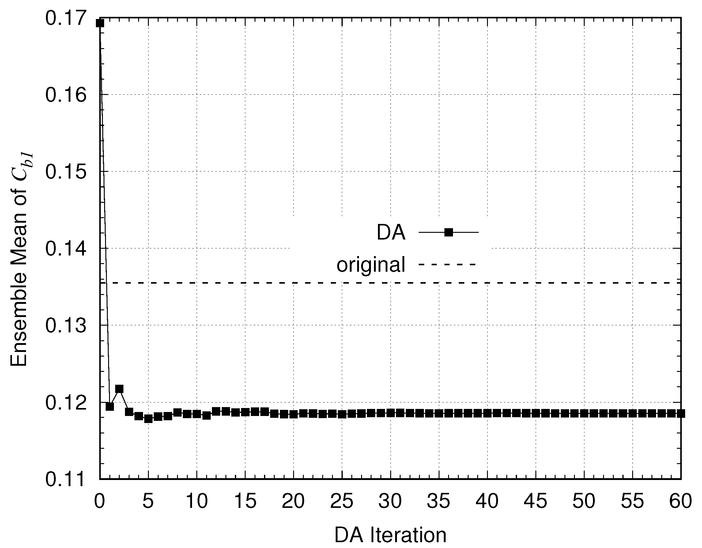
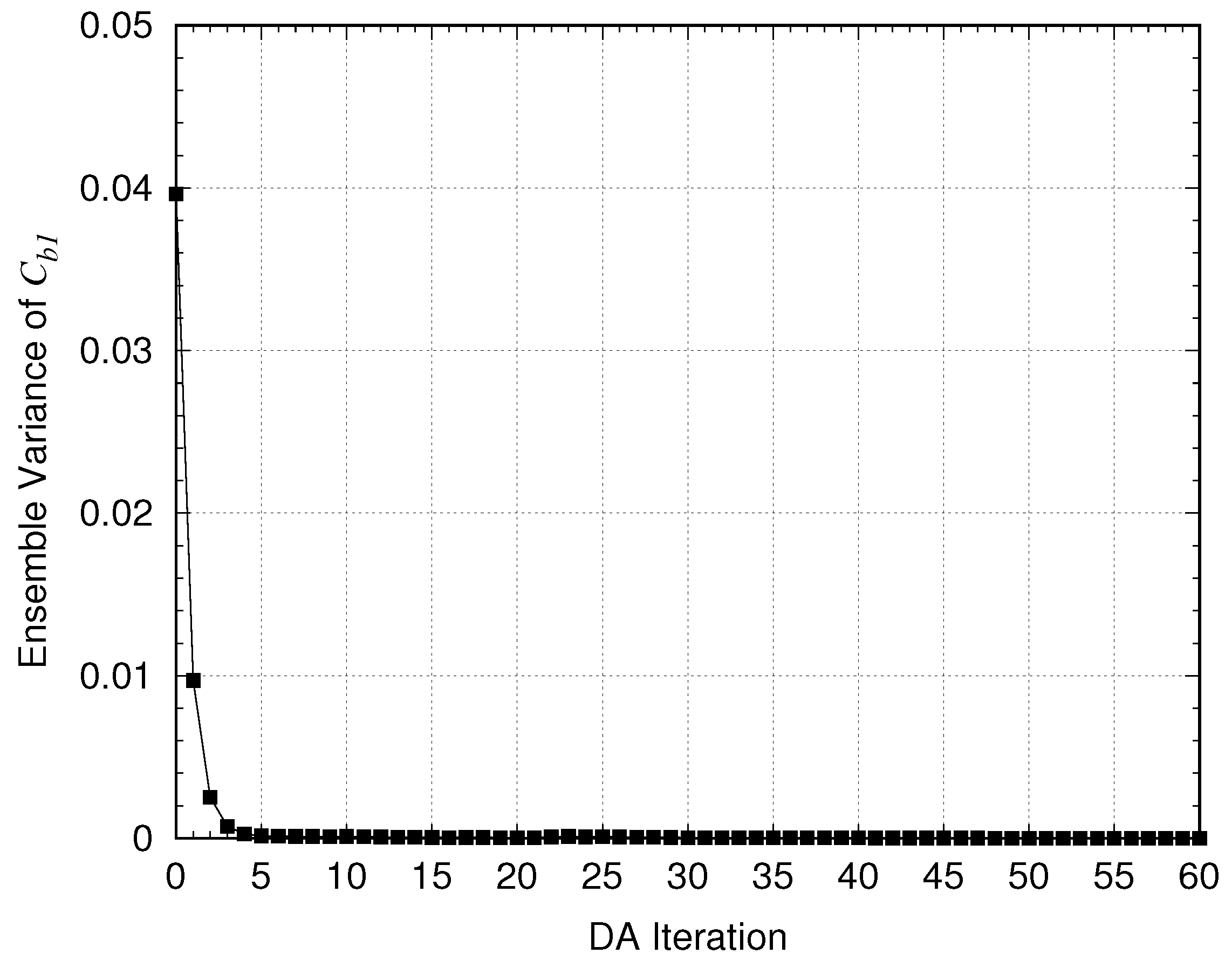
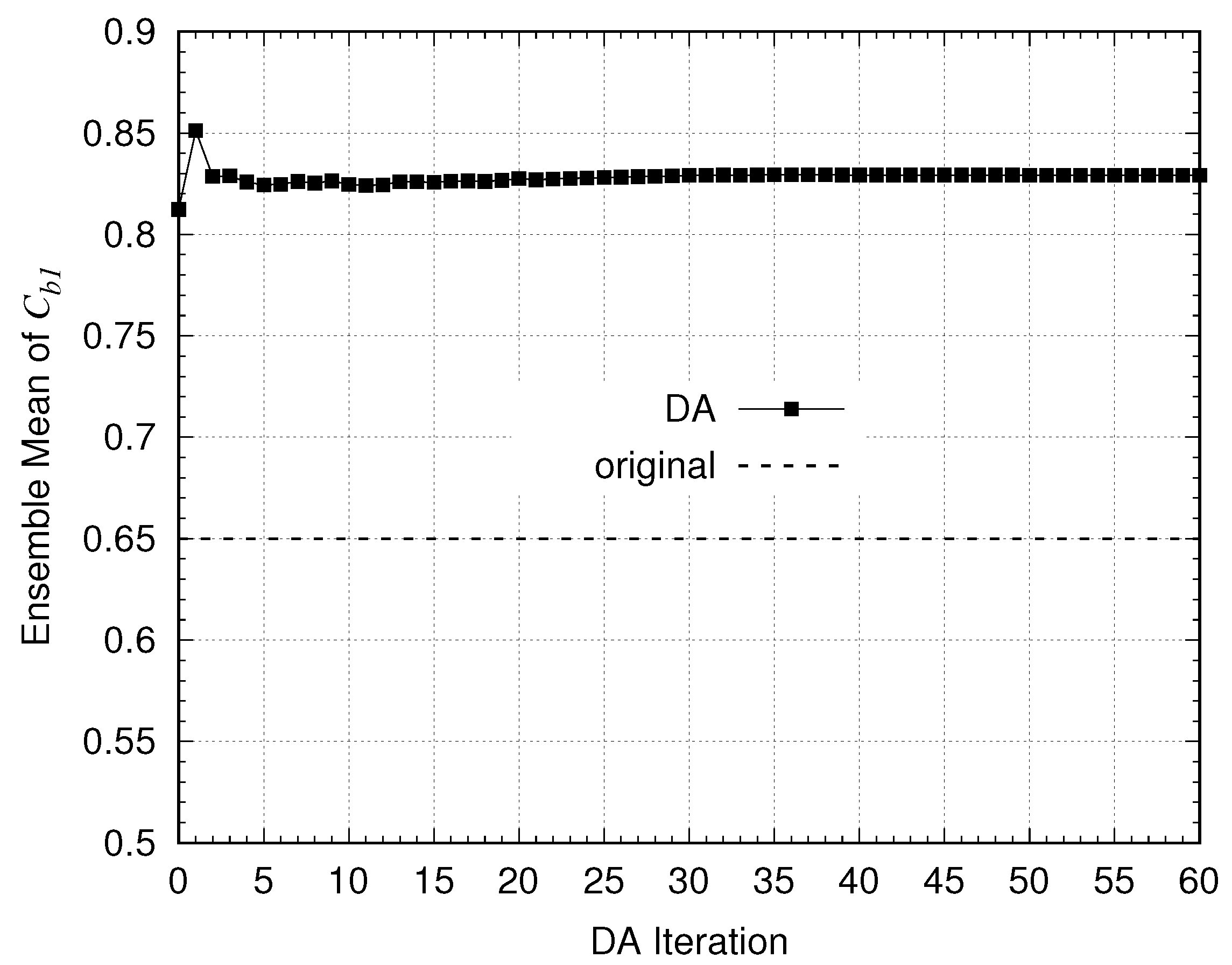
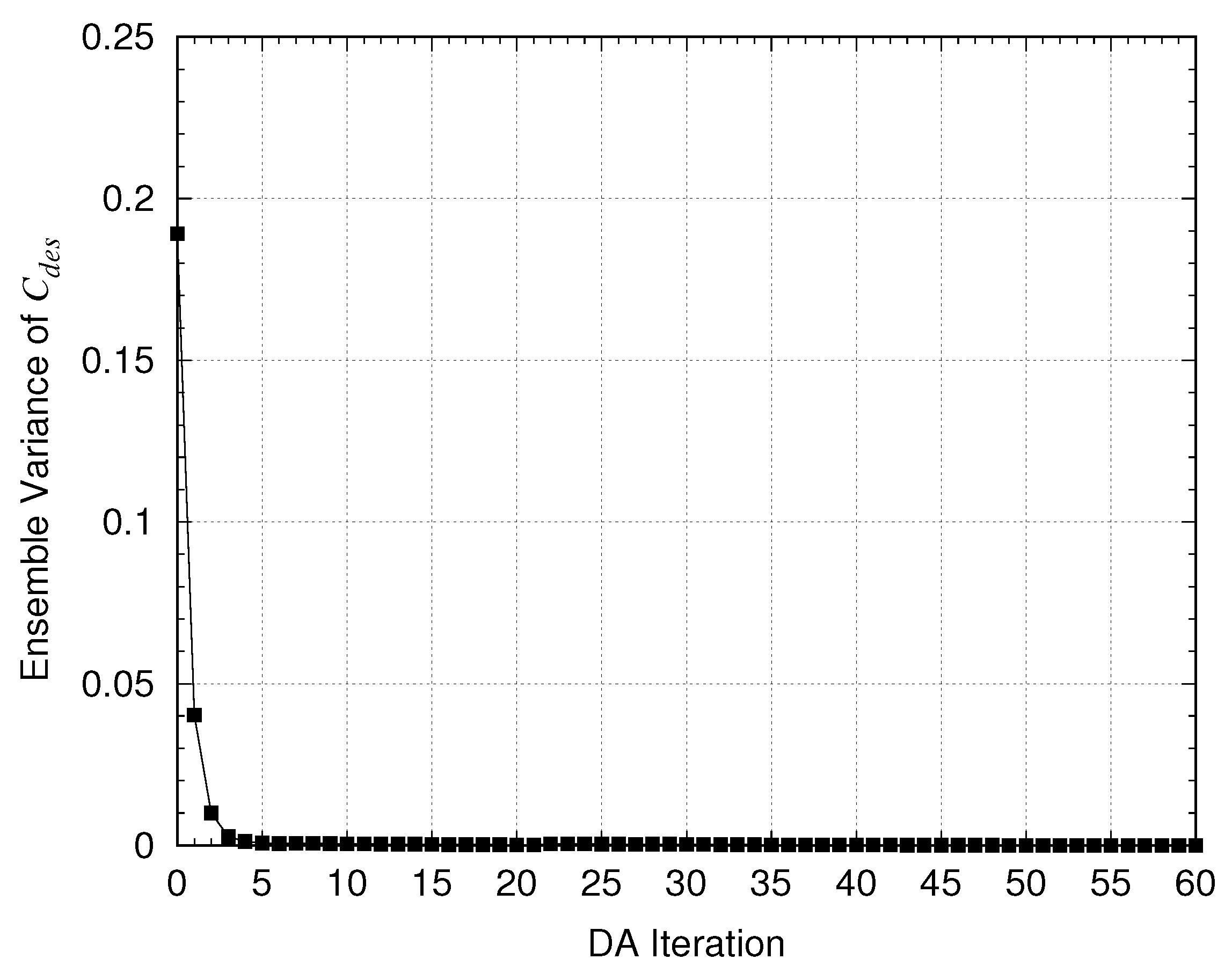
Figure 5 and Figure 6 show the history of the ensemble mean and variance for C b 1 . Similarly, Figure 7 and Figure 8 show the history of the ensemble mean and variance for C d e s . It can be observed that both parameters converged to constant values after approximately five iterations of data assimilation. Additionally, the variance decreased monotonically as the number of data assimilation iterations increased. Therefore, it can be concluded that the parameters were tuned through data assimilation. The average values of these two parameters after the 60th data assimilation iteration is regarded as the “tuned parameters.”
Table 1 compares the default parameters with the tuned parameters. While C b 1 decreased by approximately 12.5 % , C d e s increased by approximately 27.5 % . The slight reduction in C b 1 indicates a minor decrease in the rate of turbulent viscosity production. In contrast, the increase in C d e s suggests an increase in the scale of the eddies modeled as turbulent viscosity. Consequently, the overall turbulent viscosity of the airflow is expected to increase. Moreover, the increase in turbulent viscosity and the enlargement of the modeled vortex scale suppress small-scale vortex motion in the cylinder’s wake.

3.3. Comparison of Turbulent Viscosity Coefficients in Flow Fields

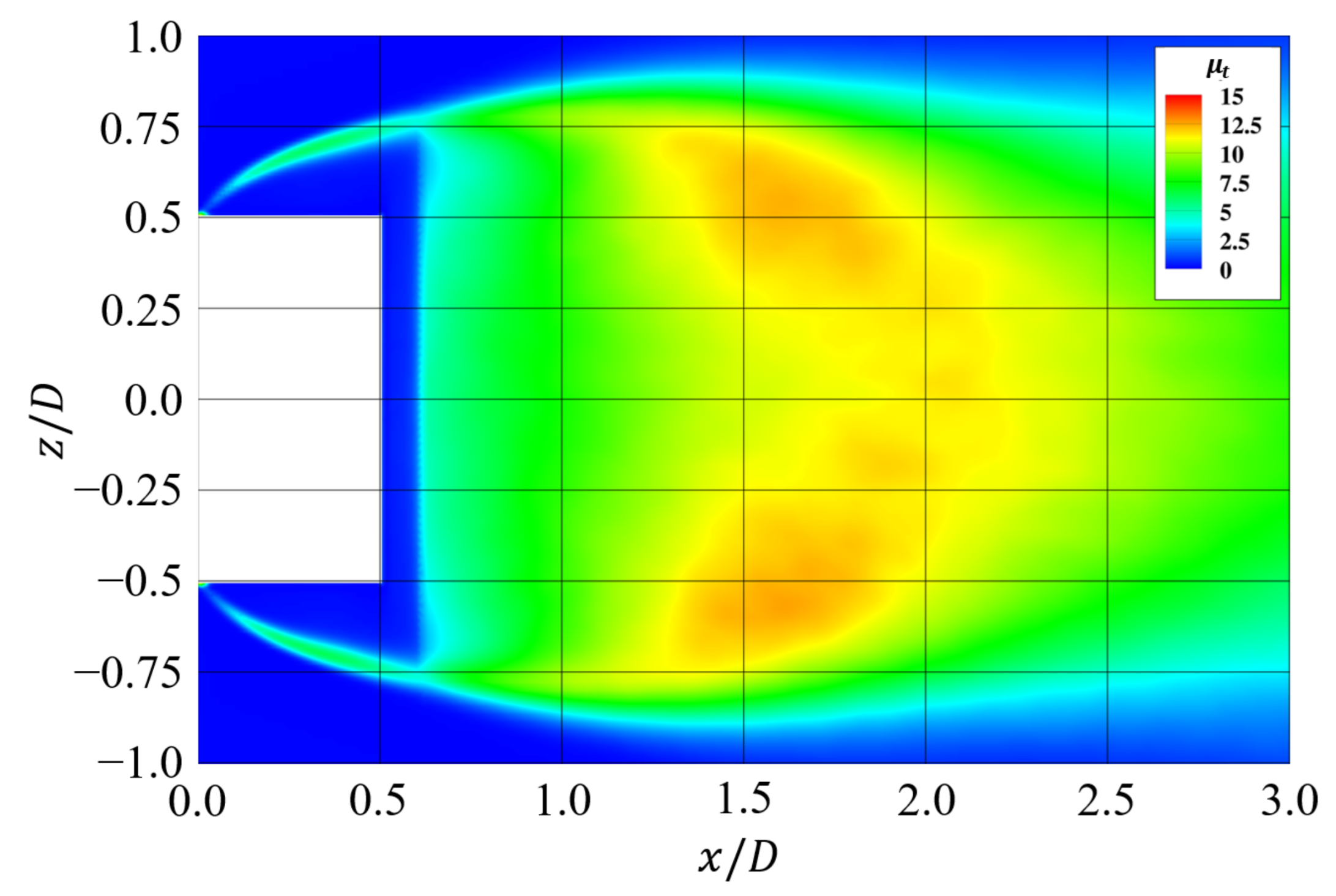
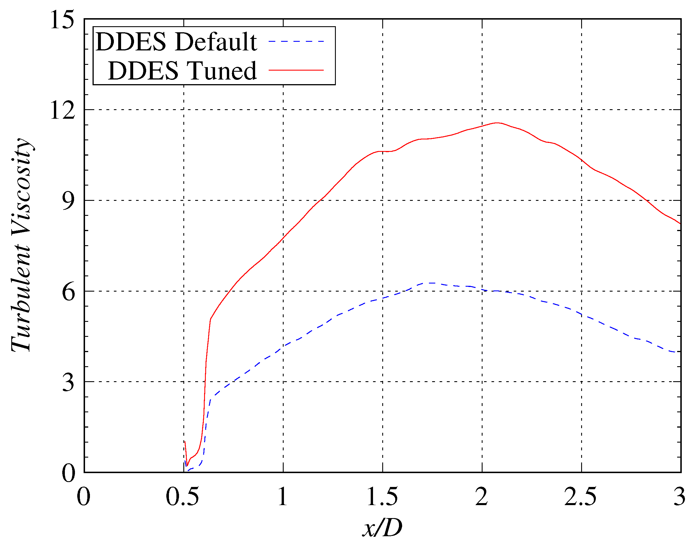
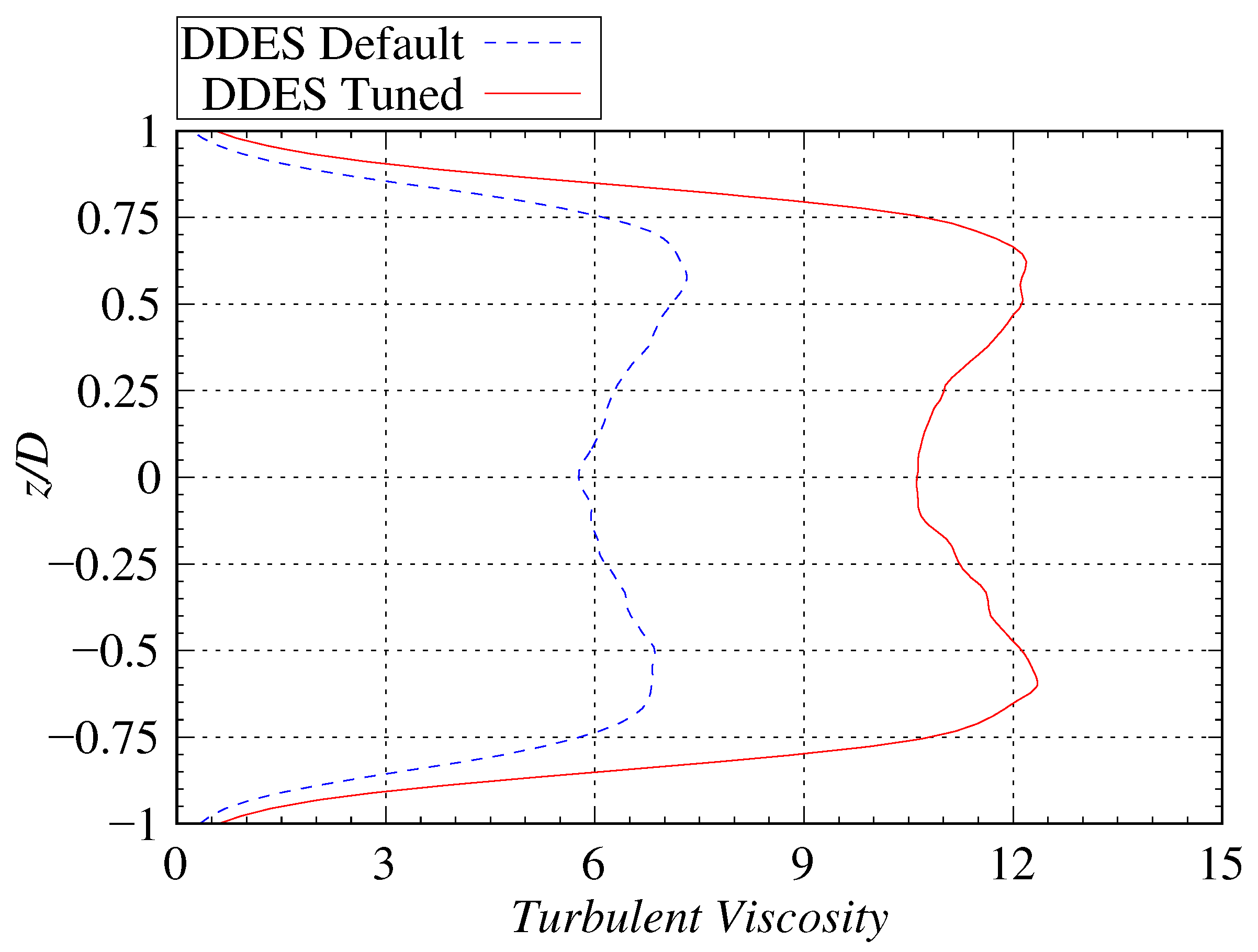
Figure 9 and Figure 10 show the distribution of turbulent viscosity coefficients in the x-z plane ( a t y / D = 0 ) passing through the center axis of the cylinder for simulations using the default parameters and tuned parameters, respectively. Figure 11, Figure 12 and Figure 13 depict the profiles of turbulent viscosity coefficients along the center axis of the cylinder, the z axis on the side surface of the cylinder ( x / D = 0.25 ) and the z axis in the wake region ( x / D = 1.5 ) , respectively. Examining the distribution of turbulent viscosity coefficients in the x-z plane, it can be observed that the turbulent viscosity coefficient is low near the cylinder wall and increases sharply outside this region. This sharp increase is attributed to the doubling of the grid size in this region, which consequently doubles the size of the vortices modeled by the SGS model. As a result, a significant gap in the turbulent viscosity coefficient arises. Focusing on the turbulent viscosity coefficients on the side surface of the cylinder, the parameter tuning increases the turbulent viscosity coefficient in the range 0.6 < z / D < 0.7 by approximately a factor of two. As mentioned above, a decrease in C b 1 is associated with a reduction in the turbulent viscosity coefficient, while an increase in C d e s contributes to its increase. Therefore, the significant increase in the turbulent viscosity coefficient suggests that the value of C d e s has a substantial impact on the flow field. The profile of the turbulent viscosity coefficient along the cylinder’s center axis shows that the gap in turbulent viscosity coefficient at x / D = 0.6 , caused by grid expansion, becomes larger with parameter tuning. The results with tuned parameters show values approximately 1.7 times higher than those with the default parameters. In the region x / D > 0.6 , the turbulent viscosity coefficient is generally higher with the tuned parameters than with the default parameters. In the z-axis profile at x / D = 1.5 , a difference of approximately two times is observed in the values of the turbulent viscosity coefficient. Thus, it can be concluded that the parameter tuning also increases the turbulent viscosity coefficient on the rear side of the cylinder. Overall, the results indicate that the increase in C d e s due to parameter tuning has a significant impact on flow in the recirculation bubble. Although parameter tuning increased the value of the turbulent viscosity coefficient, the distribution did not exhibit notable qualitative changes. This suggests that the tuned parameters, which are uniform throughout the computational domain, do not induce localized changes in the flow.

3.4. Comparison of Reynolds Stress Components u w / U 2

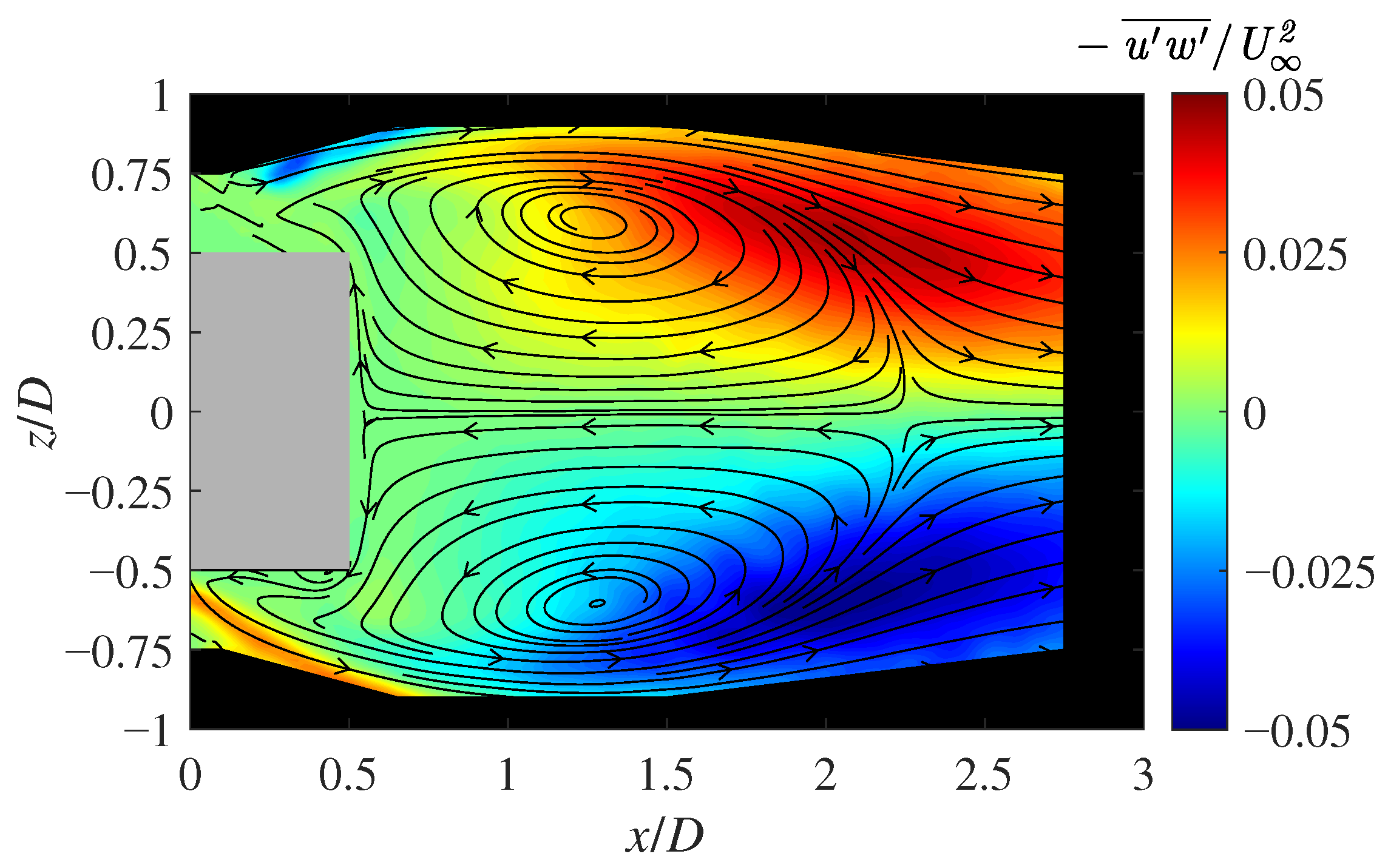
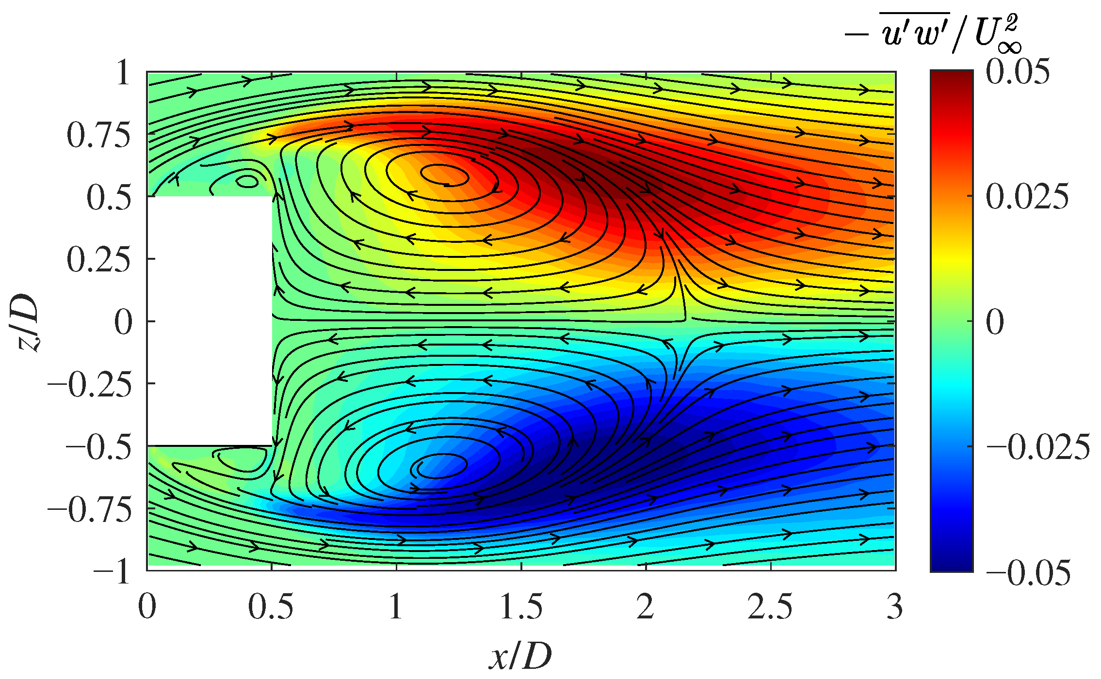
Figure 14, Figure 15 and Figure 16 show the Reynolds stress components u w / U 2 in the x-z plane through the center axis of the cylinder obtained from PIV measurements, simulation using default parameters, and simulation using tuned parameters, respectively. Streamlines illustrating the time-averaged velocity distribution were added to each figure. The PIV measurement shows no significant distribution near the cylinder and a large distribution around the outer edge of the recirculation bubble, downstream from the vortex center. However, in both simulation cases, a large distribution is shown around the outer edge of the recirculation bubble upstream from the vortex center, suggesting that the separated shear layer is stronger than in the wind tunnel testing. Comparing the two simulation cases, the tuned parameters decreased Reynolds stress in the separated shear layer upstream from the vortex center while increasing Reynolds stress near the outer edge of the recirculation bubble. This phenomenon can be attributed to the increase in C d e s damping the motion of small-scale vortices. In the vicinity of the shear layer separation dominated by small-scale fluctuations, this suppression of fluctuations decreased Reynolds stress. Conversely, downstream from the vortex center, larger-scale fluctuations dominate, and suppressing small-scale fluctuations reduces minor oscillations, enhancing the correlation between the large scale velocity fluctuations u and w , thereby increasing Reynolds stress.

3.5. Comparisons of Velocity Distribution at Wake Flow

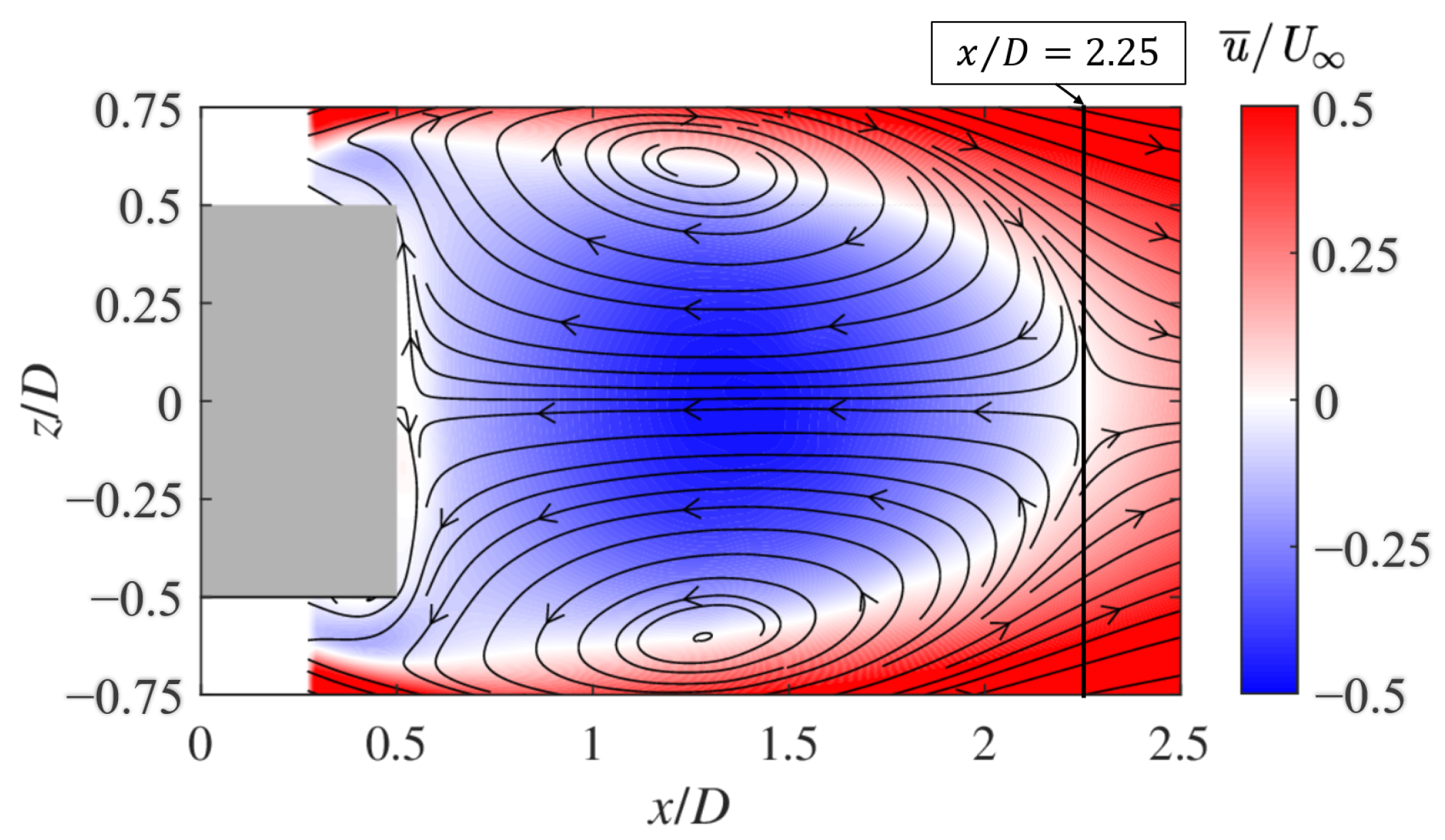
Figure 17, Figure 18 and Figure 19 show the results of the velocity distribution from the PIV measurement data, the simulation using the default parameters, and the simulation using the tuned parameters, respectively. Examining the length of the recirculation bubble, the PIV measurement data indicate x / D = 2.25 , the default parameter simulation results indicate x / D = 2.15 , and the tuned parameter simulation results indicate x / D = 2.23 . These results demonstrate that parameter tuning brought the size of the recirculation bubble closer to the PIV measurement data, indicating an improvement in simulation accuracy.
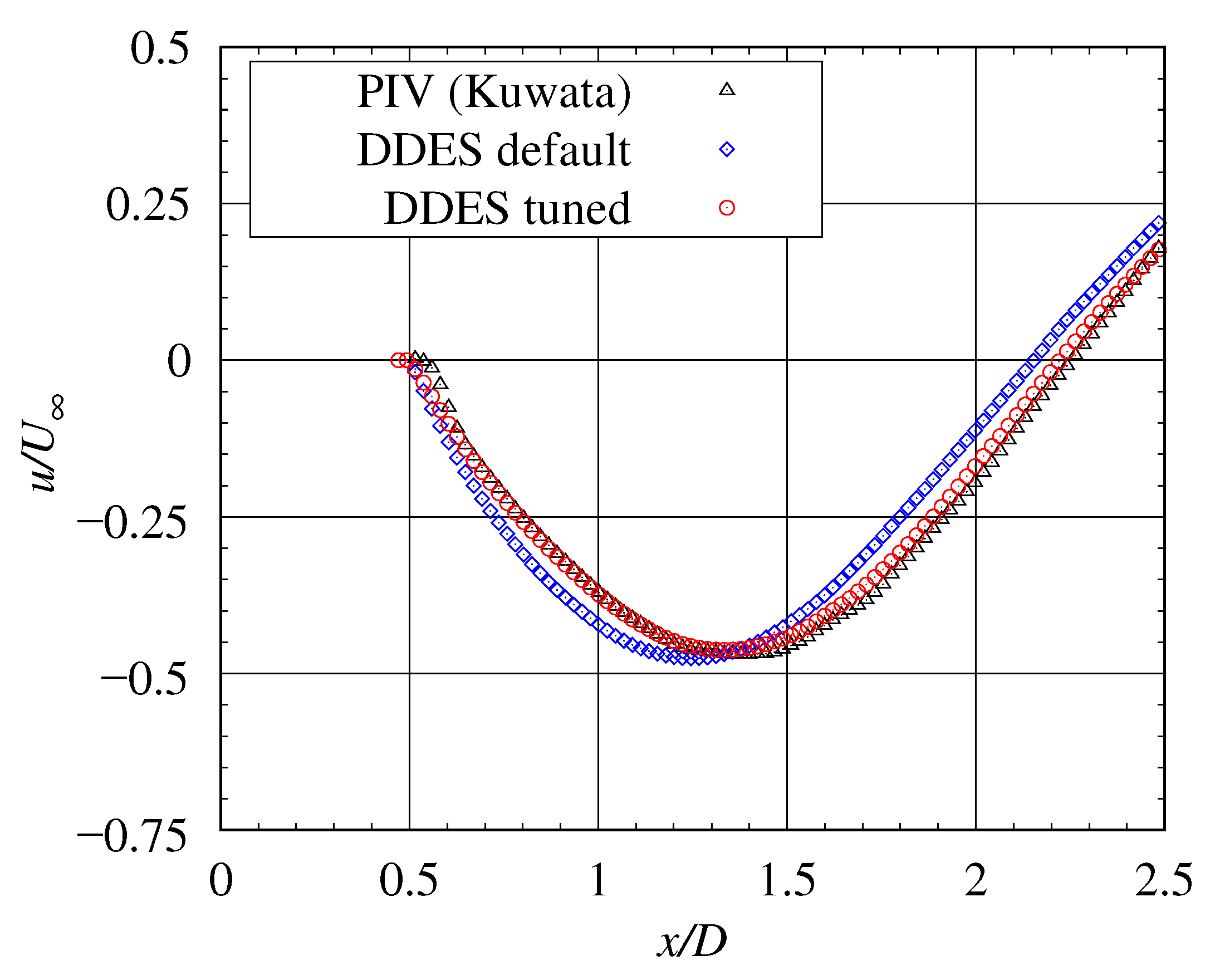
Figure 20 shows the profile of the x-direction velocity u along the center axis of the cylinder. Although the results with the default parameters reproduce the velocity distribution to a certain extent, the parameter tuning enabled a simulation that closely matches the PIV measurement data. In particular, in the region near the back surface of the cylinder ( 0.5 < x / D < 1.0 ) , the velocity gradient nearly coincides with the PIV measurement data.
Table 2 displays the position and value of the minimum velocity for the PIV measurement and each simulation. Parameter tuning brought the location of the minimum velocity and the value of the minimum velocity closer to those observed in the PIV measurement data.
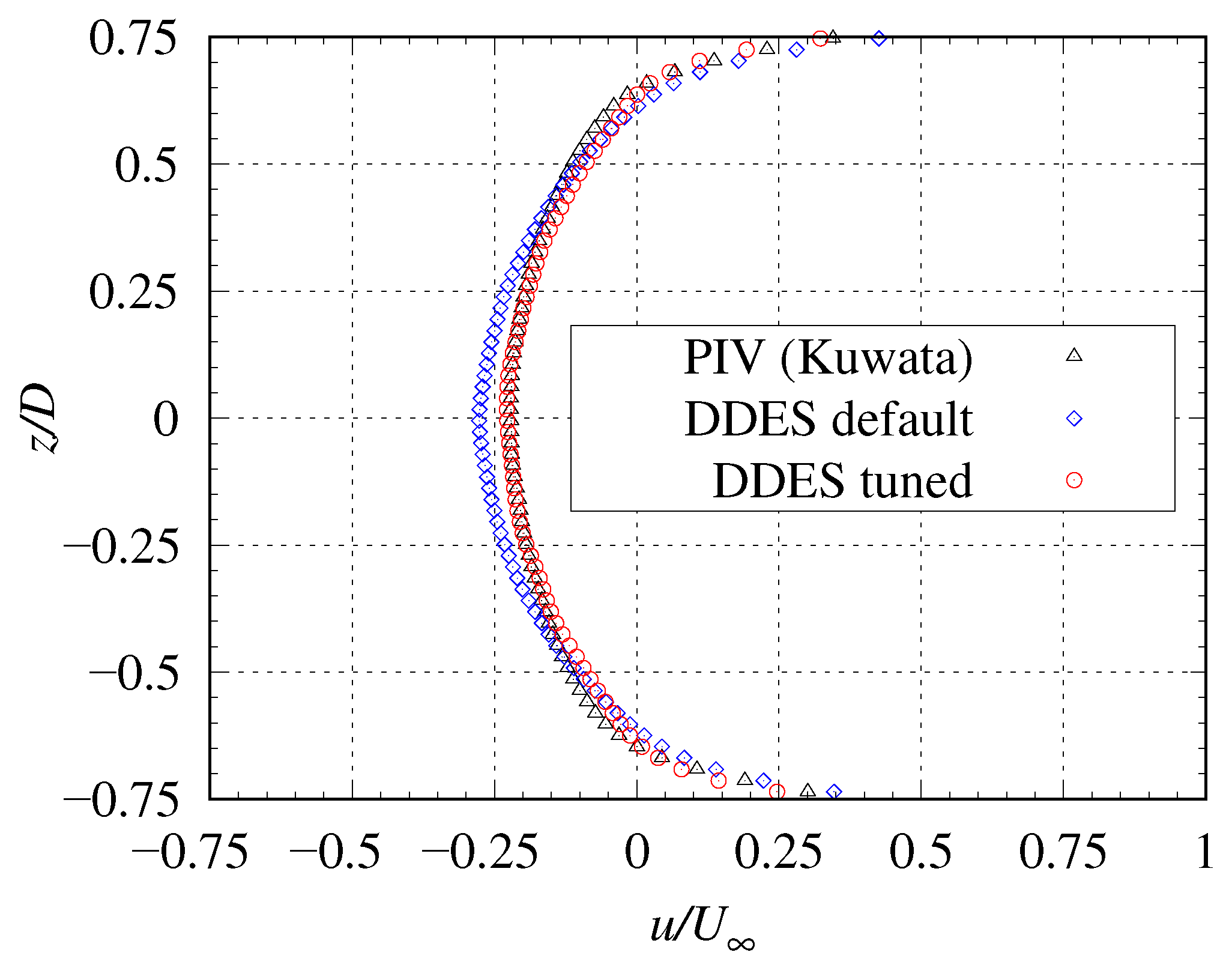
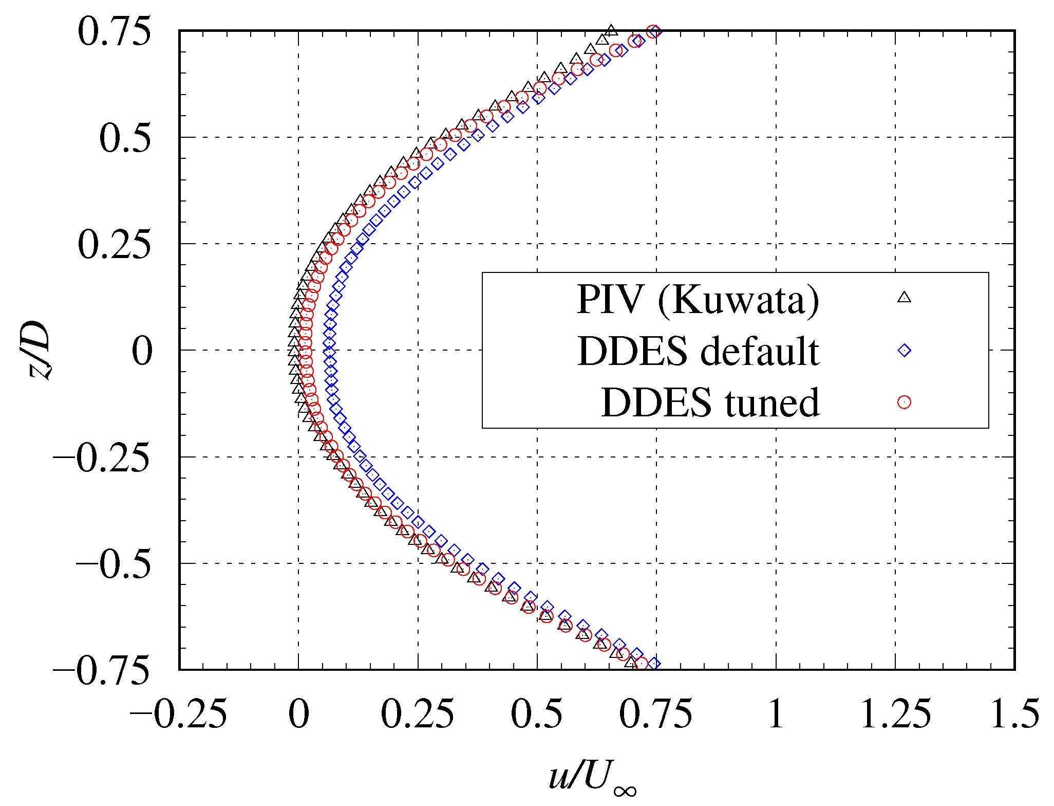
Figure 21, Figure 22 and Figure 23 present the z-axis profiles of u/U at three locations: near the back surface of the cylinder ( x / D = 0.75 ), the location with the minimum velocity in the PIV measurement data ( x / D = 1.4 ), and near the end of the recirculation bubble in the PIV measurement data ( x / D = 2.25 ).
In the region near the back surface of the cylinder ( x / D = 0.75 ) , the velocity distribution shows an overall improvement, although slight errors remain in the range 0.5 < | z / D | < 0.75 . At x / D = 1.5 , the velocity distribution closely matches the PIV measurement data, both near the center axis of the cylinder and at the outer edge of the recirculation bubble. At x / D = 2.25 , as inferred from the comparison of the length of the recirculation bubble, minor errors remain in the velocity near the center axis of the cylinder. However, the results using the tuned parameters overall exhibit values closer to the PIV measurement data. Therefore, parameter tuning significantly improved the simulation accuracy of the time-averaged velocity distribution in the recirculation bubble of the cylinder wake.

3.6. Velocity Fluctuations in the Wake of the Cylinder

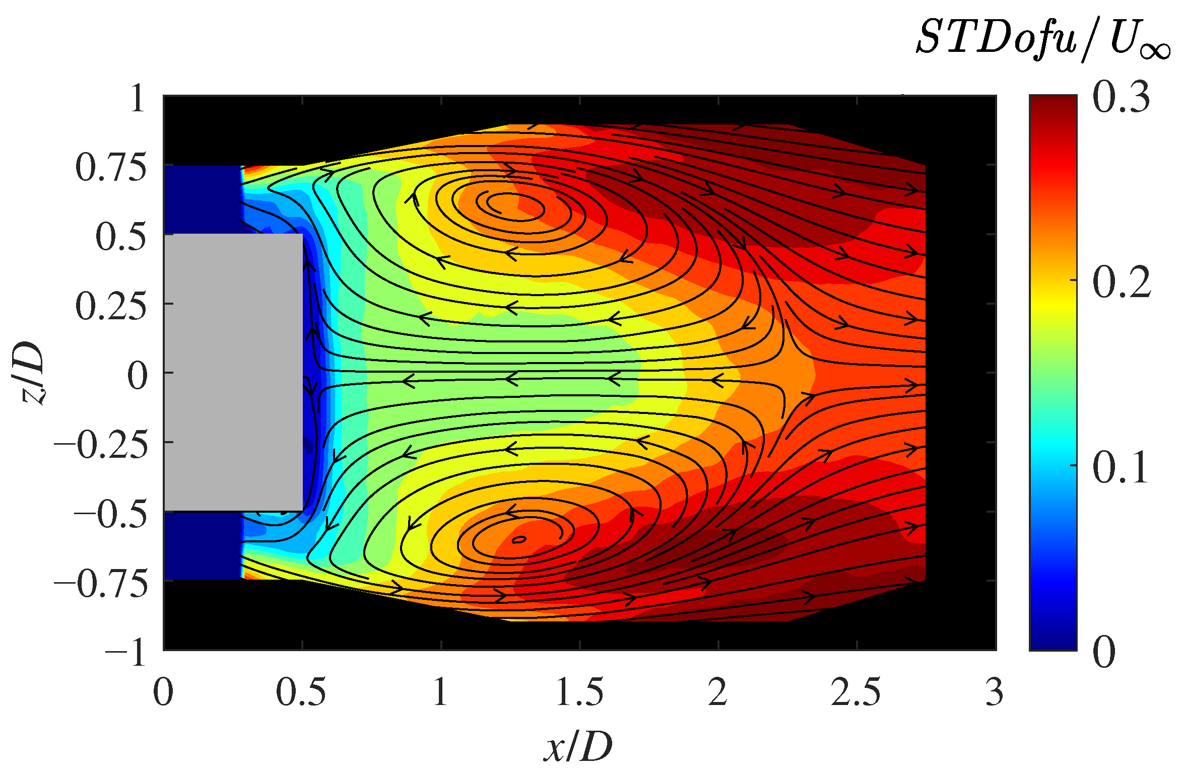
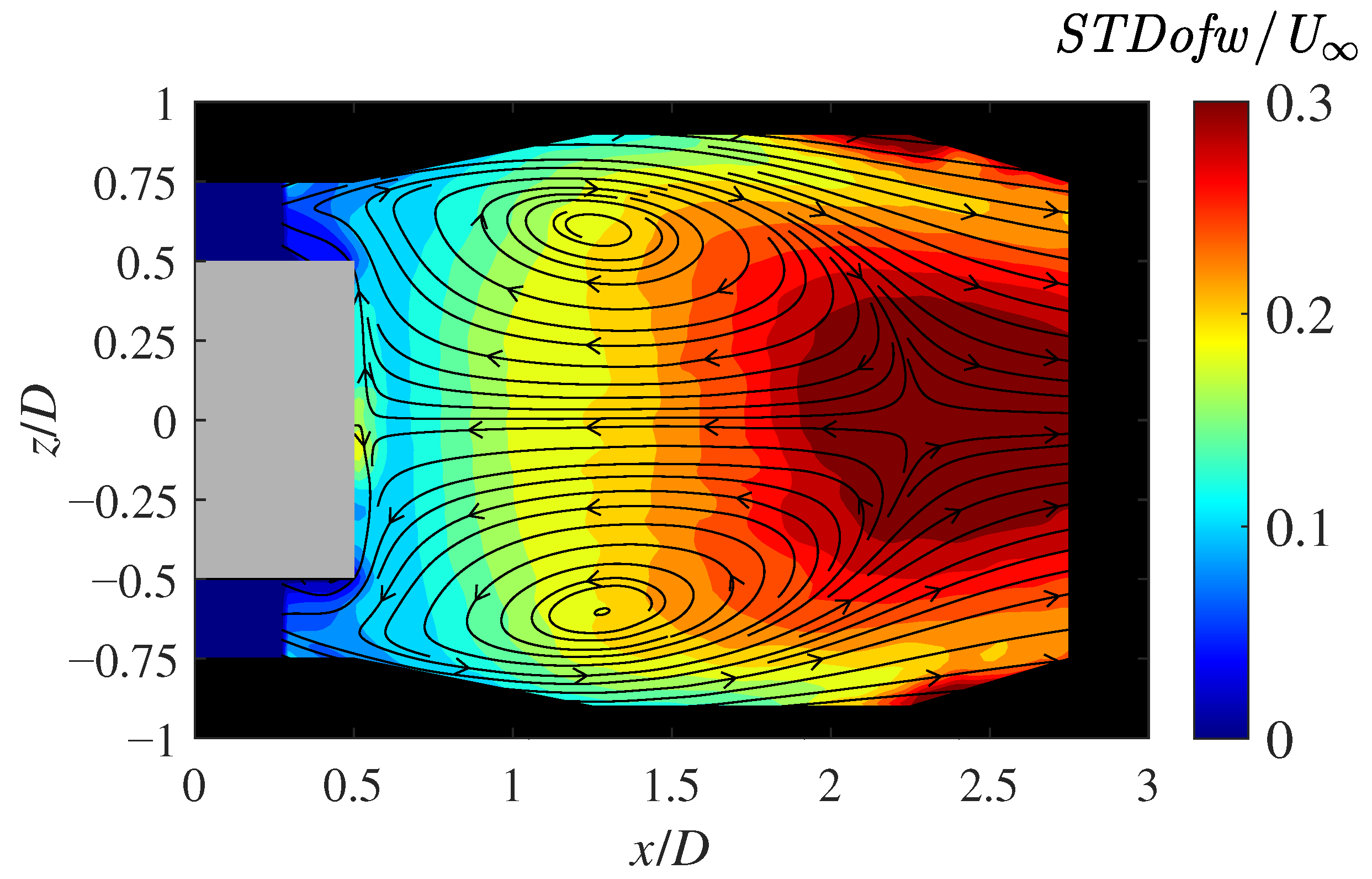
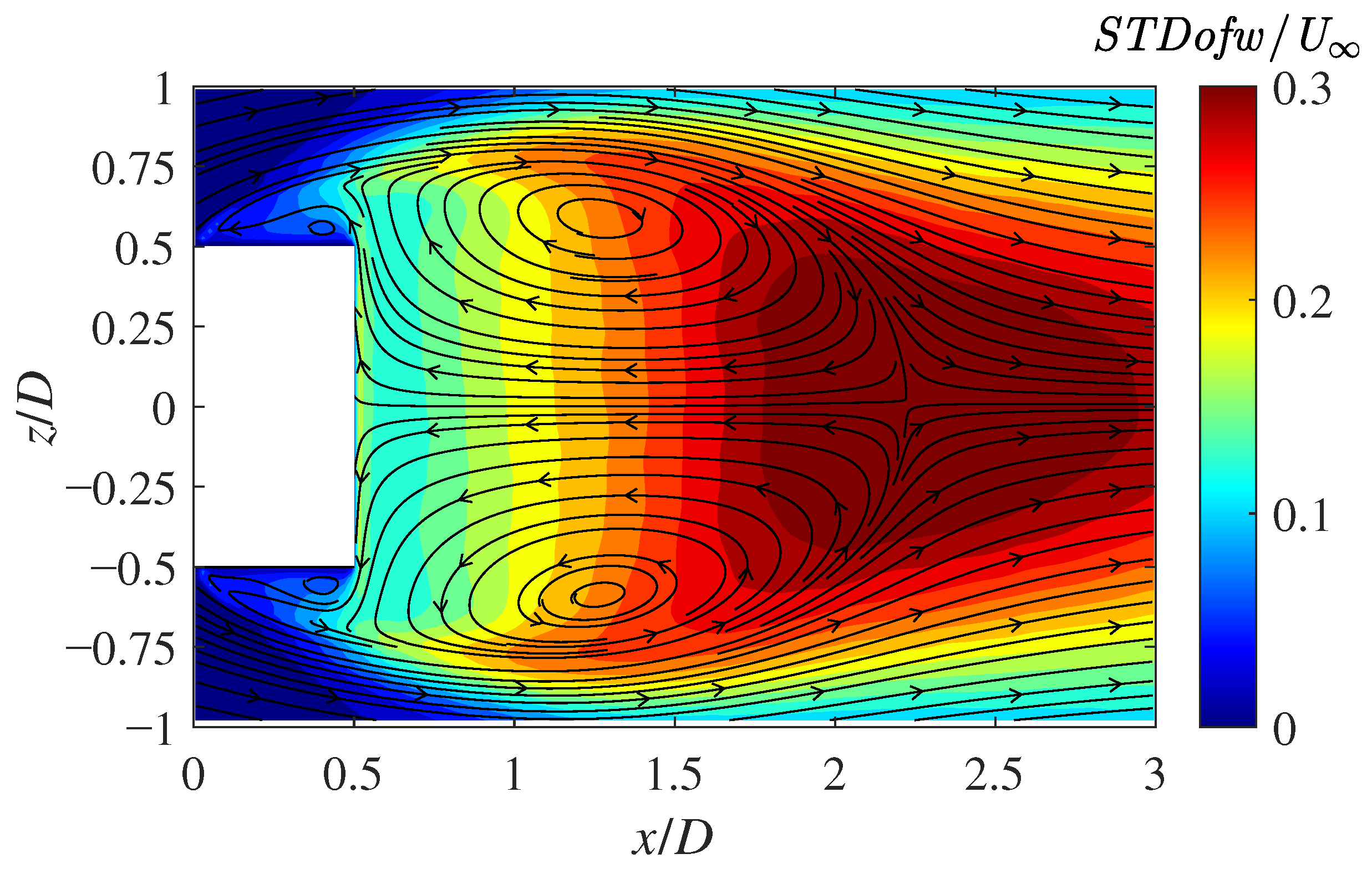
Figure 24, Figure 25 and Figure 26 show the standard deviation distributions of the streamwise velocity component u obtained from the PIV measurement data, the simulation using default parameters, and the simulation using tuned parameters, respectively.
Then, Figure 27, Figure 28 and Figure 29 show the standard deviation distributions of the spanwise velocity component w obtained from the PIV measurement data, the simulation using default parameters, and the simulation using tuned parameters, respectively.
When examining the x-direction velocity u, the PIV measurement data exhibit significant fluctuations near the edge of the recirculation bubble ( 1.5 < x / D < 2.25 , 0.5 < | z / D | < 0.8 ). In both simulation cases, large fluctuations are observed upstream ( x / D 0.5 ) compared to the PIV measurement data. However, the overall distribution is like that of the PIV data. It is worth noting that the simulation with tuned parameters shows a slightly downstream shift in the region of large fluctuations. For the z-direction velocity w, the PIV measurement data reveal an increasing trend in fluctuations with distance from the rear of the cylinder, peaking near the downstream stagnation point of the recirculation bubble ( x / D > 2.0 , | z / D | < 0.5 ) . While both simulation cases show a generally similar trend, the distribution near the centers of the two vortices in the recirculation bubble qualitatively differs. In both simulations, regions of strong fluctuations extend upstream like “spikes,” a feature not observed in the PIV data. Although quantitative differences are less pronounced, the weak fluctuation region near the cylinder back surface is slightly broader in the tuned parameter case, and the strong fluctuation region around the end of recirculation bubble shifts downstream.
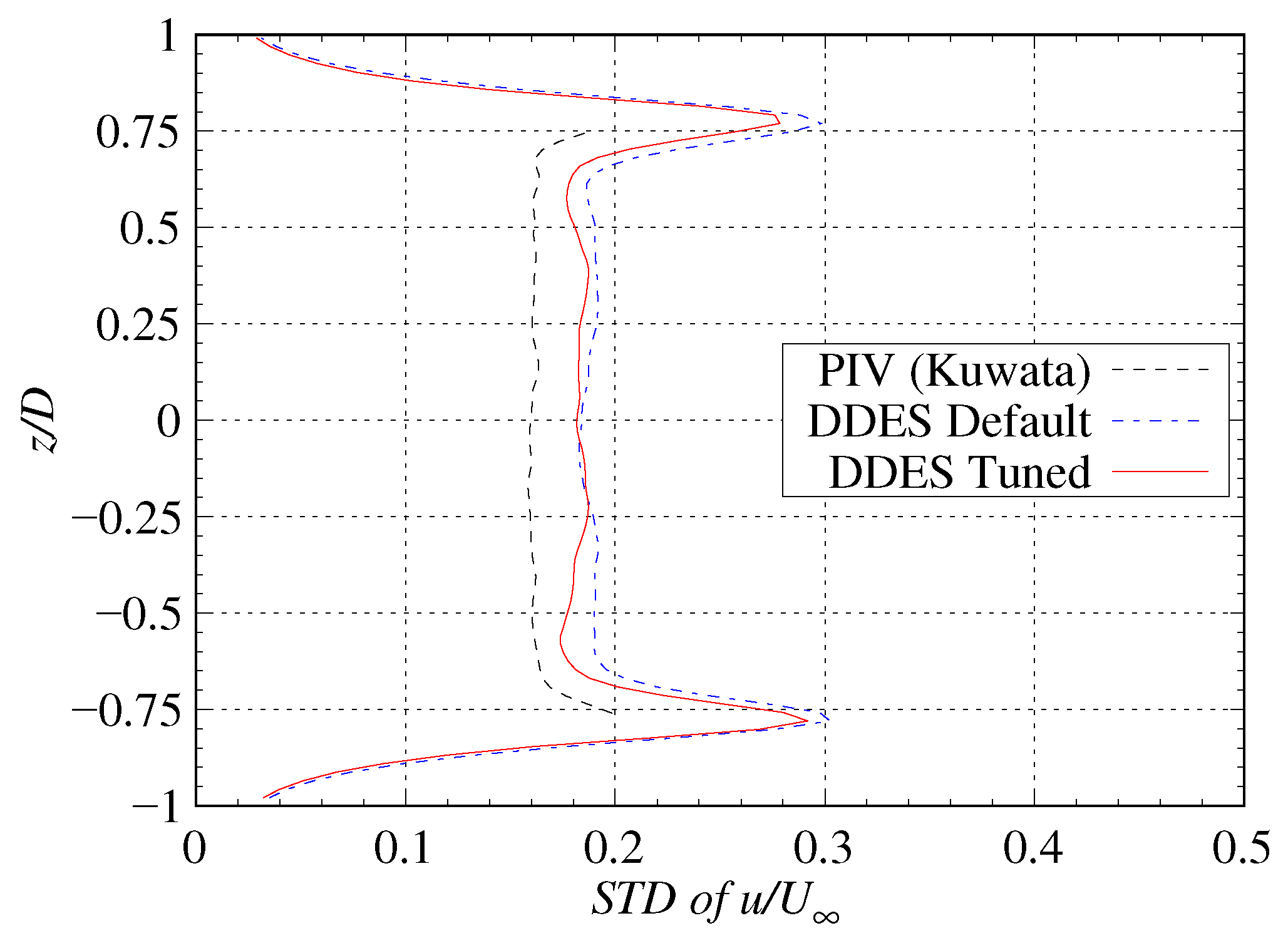
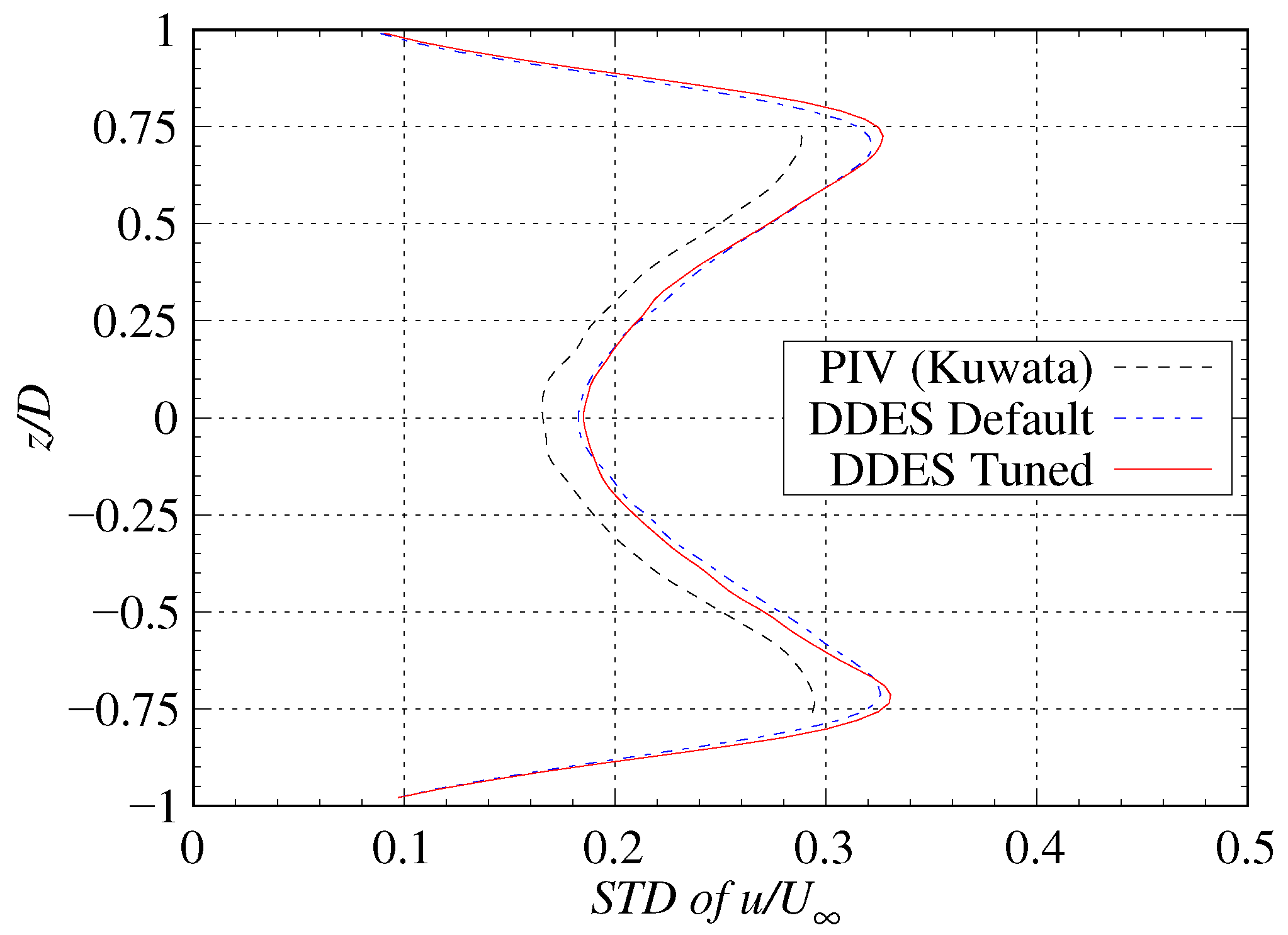
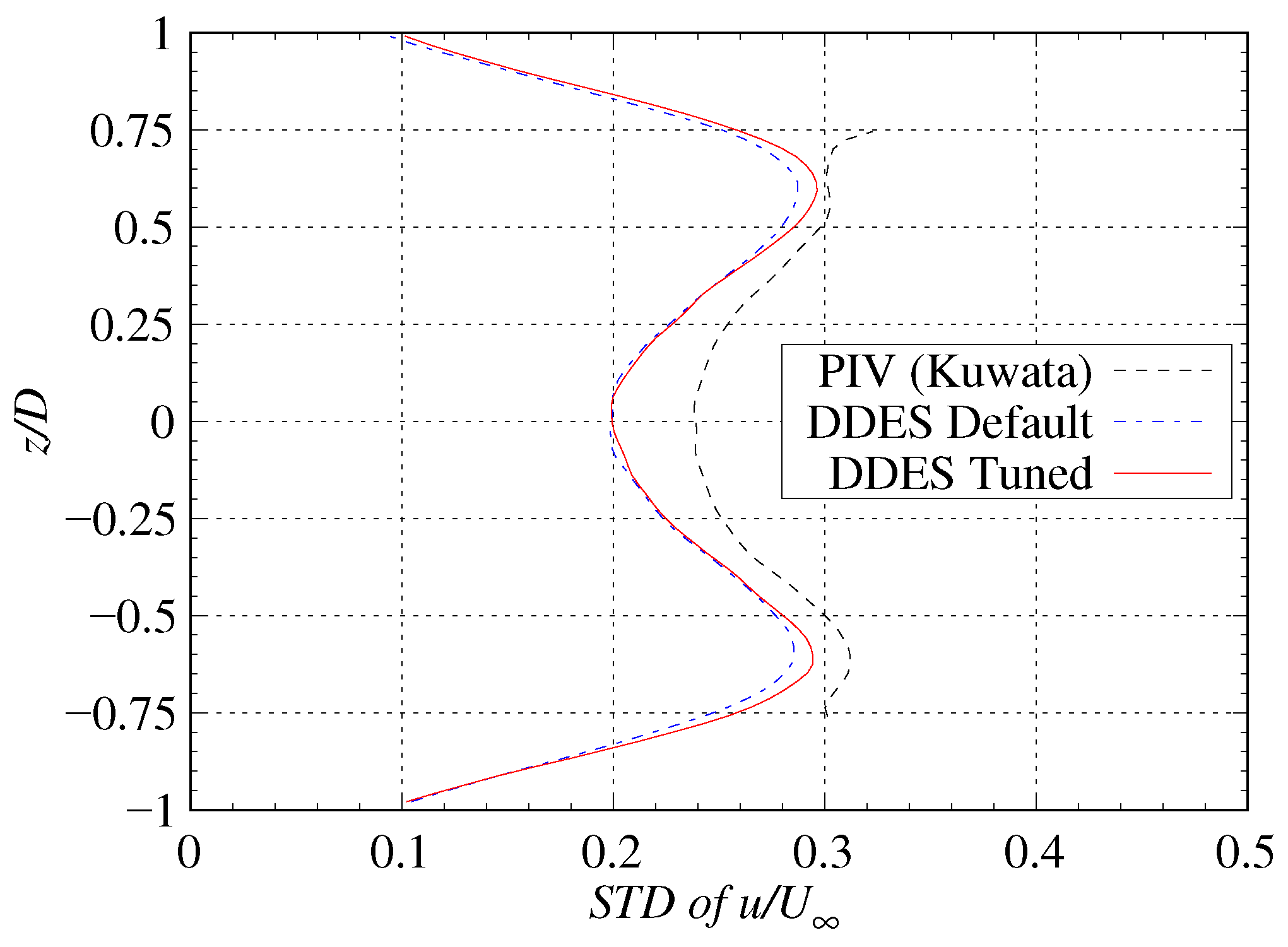
Figure 30, Figure 31 and Figure 32 show the z-axis profiles of the standard deviation of the streamwise velocity component u at three locations: x / D = 0.75 , x / D = 1.5 , and x / D = 2.25 . For the PIV measurement data, regions with | z / D | > 0.75 , where data reliability is low, were excluded from the comparison.
At x / D = 0.75 , the profile shows a peak fluctuation at | z / D | = 0.75 , with fluctuations stabilizing at values between 0.16 and 0.19 closer to the center axis of the cylinder, despite slight oscillations. The tuned parameter results show weaker fluctuations compared to the default parameter results, which align more closely with the PIV measurements. This suggests that parameter tuning suppressed velocity fluctuations near the cylinder back surface, likely due to the damping of small-scale motions caused by the increase in C d e s . At x / D = 1.5 , the fluctuations increase with the distance from the center axis of the cylinder, peak at | z / D | = 0.75 , and then decrease. Compared to the PIV measurements, the simulation results exhibit fluctuations from 0.02 to 0.03 higher throughout the profile. The parameter tuning caused only small changes, indicating a limited impact. At x / D = 2.25 , the qualitative characteristics of the distribution are similar to those at x / D = 1.5 , but the peak fluctuation occurs closer to the center axis of the cylinder at | z / D | = 0.6 . Although the PIV measurements show higher values than the simulations, the tuned parameter results are closer to the PIV data near the peak at | z / D | = 0.6 .
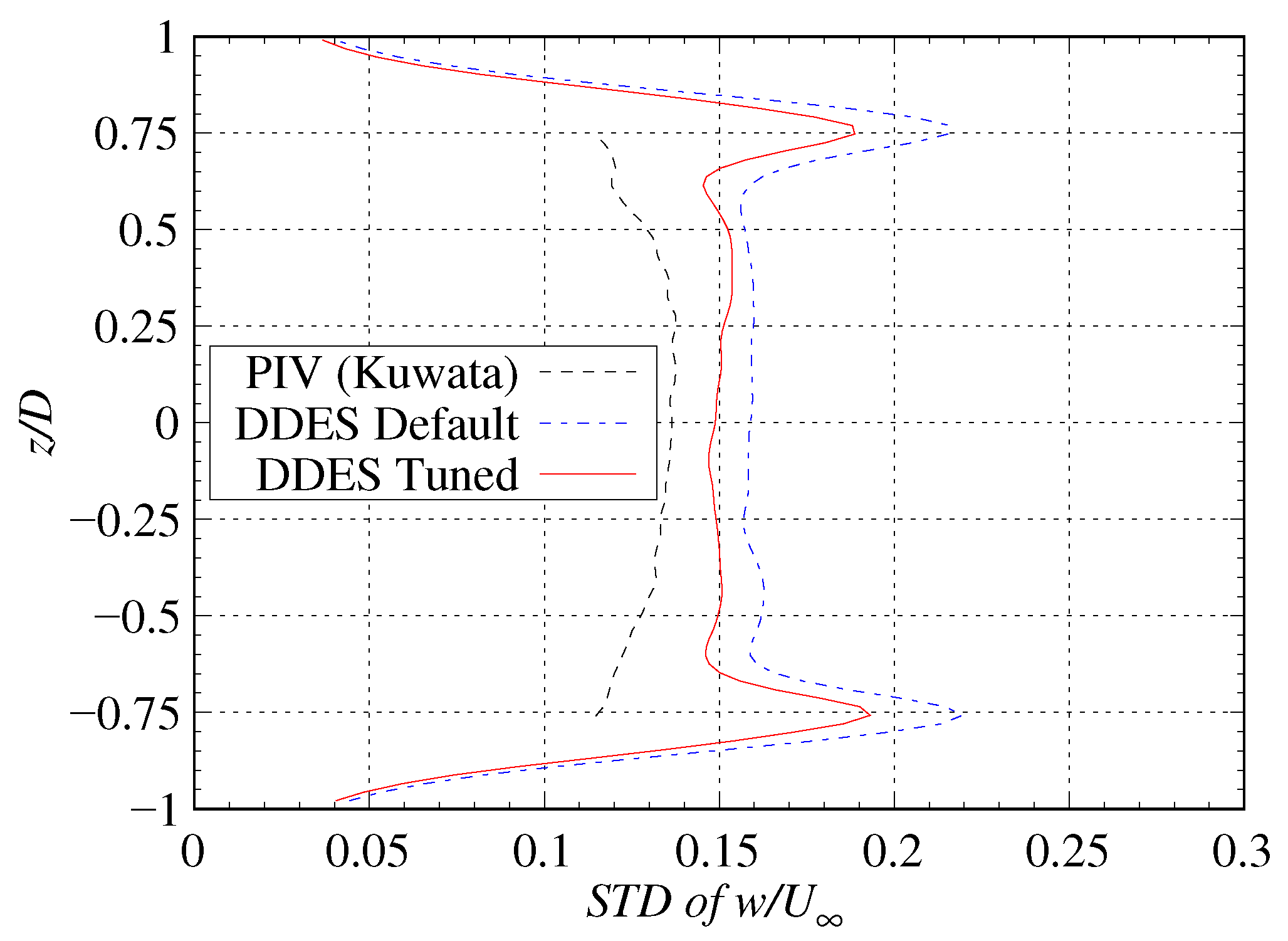
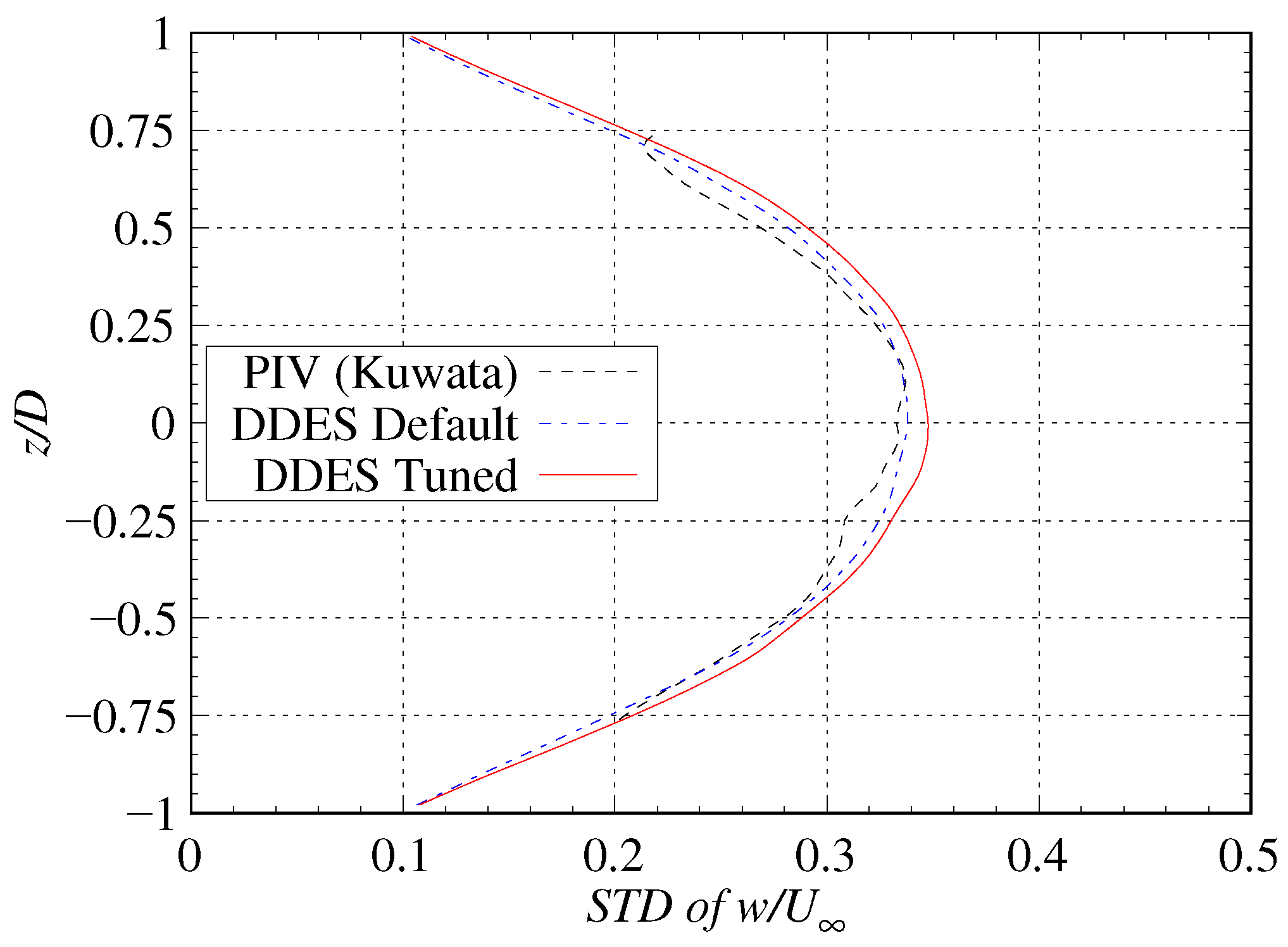
Figure 33, Figure 34 and Figure 35 show the z-axis profiles of the standard deviation of the z-direction velocity component w at x / D = 0.75 , x / D = 1.5 , and x / D = 2.25 , respectively. As for the velocity component u, the PIV data for | z / D | > 0.75 were excluded from the comparison.
At x / D = 0.75 , the simulation results show a peak at | z / D | = 0.75 , which is not present in the PIV measurements. Within the recirculation bubble ( | x / D | < 0.7 ) , the fluctuation magnitudes follow the order P I V < T u n e d P a r a m e t e r s < D e f a u l t P a r a m e t e r s , indicating that parameter tuning reduced velocity fluctuations near the back surface of the cylinder, bringing them closer to the PIV data. At x / D = 1.5 , the profiles show consistent fluctuation magnitudes within the recirculation bubble ( | z / D | < 0.6 ) . Quantitatively, the PIV measurements show smaller fluctuations compared to the simulations, with the tuned parameter results being slightly closer to the PIV data than the default parameter results. At x / D = 2.25 , the magnitude of the fluctuation peaks on the center axis of the cylinder and decreases outward. Although no qualitative differences are observed among the three cases, the tuned parameter results show slightly larger fluctuations than the default parameter results.
From the contour plots and z-axis profiles of velocity fluctuations in the cylinder wake, it is evident that parameter tuning did not cause qualitative changes in the fluctuation distribution. However, parameter tuning resulted in quantitative changes, such as reduced fluctuations near the cylinder rear and increased fluctuations downstream, indicating that the distribution of velocity fluctuations shifted slightly downstream due to parameter tuning. In this study, parameter tuning resulted in a significant increase in the value of C d e s . This change enlarged the scale of vortices treated as turbulent viscosity within the turbulent flow. Consequently, small-scale velocity fluctuations caused by flow separation at the leading edge of the cylinder were suppressed. This suppression delayed the development of velocity fluctuations, changing the generation of vortices that form the recirculation bubble slightly downstream. As a result, the elongation of the recirculation bubble observed in Section 3.5 can be attributed to this effect.

3.7. Time–Frequency Analysis of Velocity Fluctuation

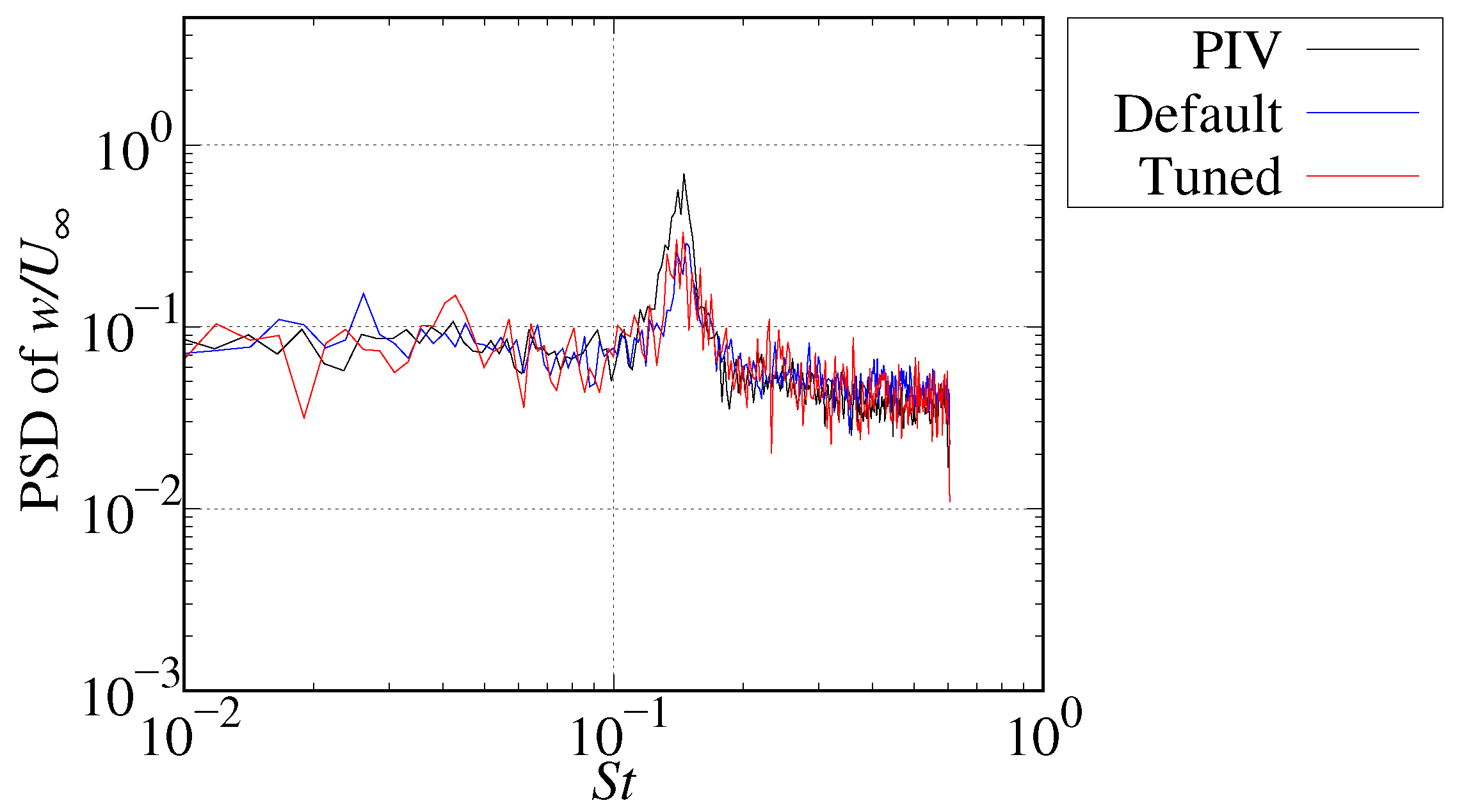
From the comparison of fluctuations in the x-direction velocity u and z-direction velocity w, distributions with strong fluctuations were identified at specific locations in the cylinder wake. Strong velocity fluctuations suggest the formation of characteristic unsteady velocity fields in these regions. To examine the spatial distribution of these unsteady velocity fields, FFT analyses of the velocity components were performed and differences between PIV measurements and the simulation results were compared. The velocity components FFT were performed for the first time, and three coordinate points were selected for comparison of the Power Spectral Density (PSD) of u and w. The selected points were: (1) near the cylinder rear where the fluctuations are weak ( x / D = 1.0 , z / D = 0.0 ) ; (2) downstream of the cylinder rear where strong fluctuations in w were observed ( x / D = 2.0 , z / D = 0.0 ) ; and (3) near the edge of the recirculation bubble where strong fluctuations in u were observed ( x / D = 2.0 , z / D = 0.65 ) . These points are referred to as Point 1, Point 2, and Point 3, respectively.
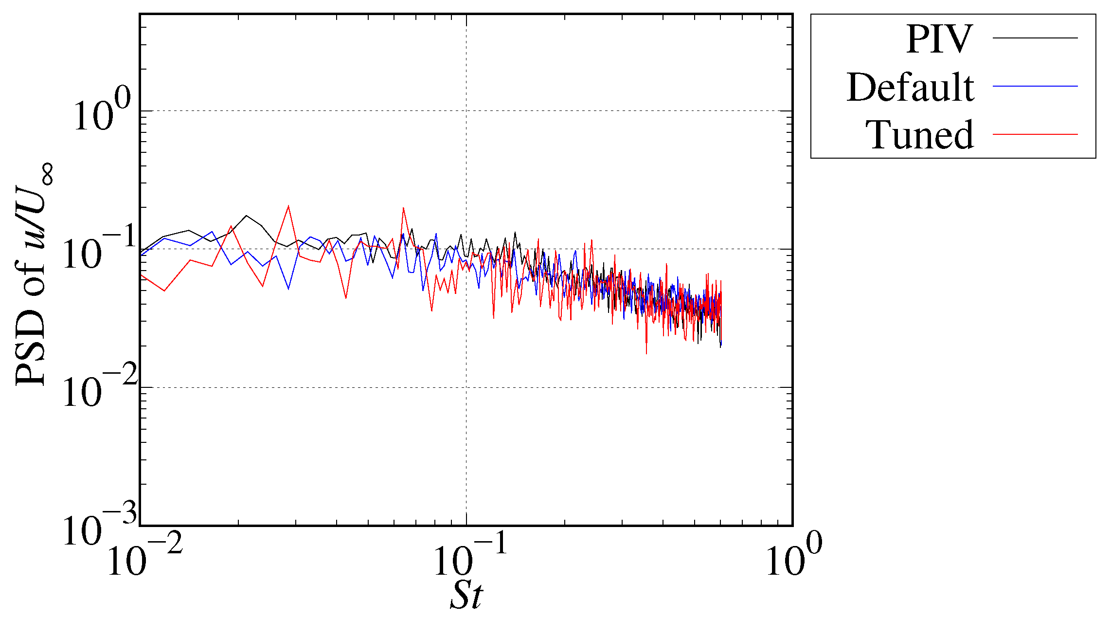
Figure 36 and Figure 37 compare the PSD obtained by FFT analyses of the x-direction velocity u and the z-direction velocity w at Point 1 ( x / D = 1.0 , z / D = 0.0 ) for the PIV measurement data, the simulation using default parameters, and the simulation using tuned parameters.
For u, all cases exhibit similar distributions, showing a decrease in PSD from low-frequency to high-frequency ranges. For w, the three cases show a distribution with a peak at S t 0.14 , indicating qualitative agreement in the fluctuation components of the flow at point 1. Quantitative differences are not observed for u, but for w, the peak value at S t 0.14 is lower in the simulations compared to the PIV measurements. Specifically, the peak value is approximately 0.7 in the PIV data, whereas it is about 0.3 in both simulation cases. Additionally, parameter tuning causes the peak position in the w PSD to shift slightly toward lower frequencies and the peak width to broaden. However, no significant differences in peak height were observed.
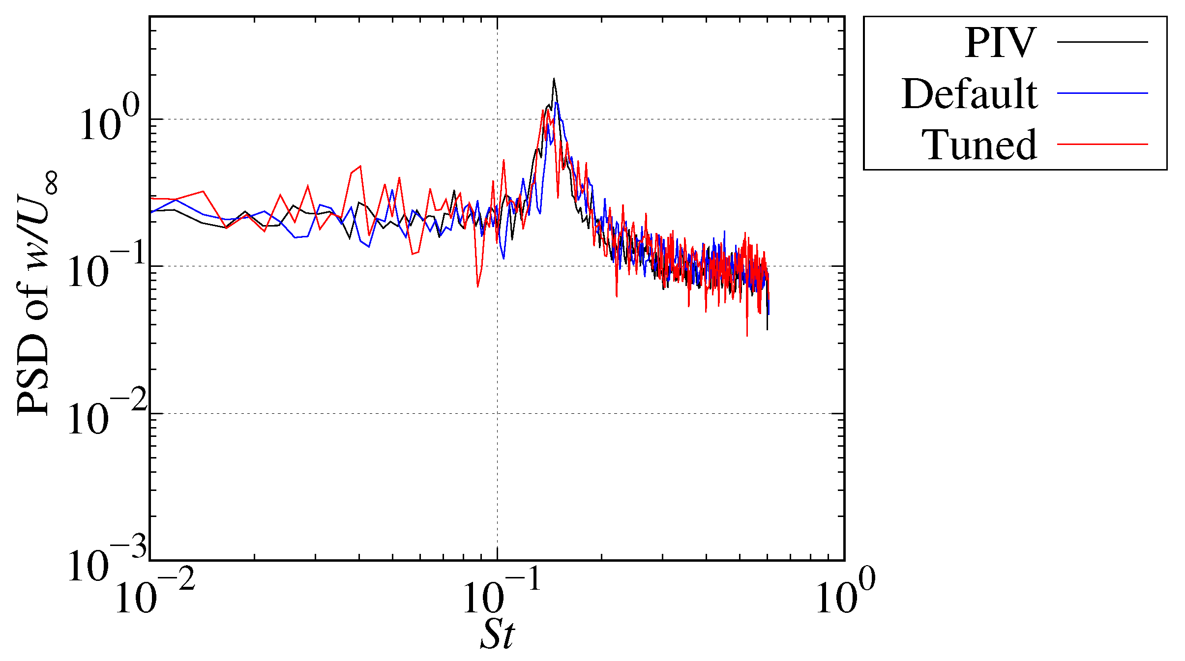
Figure 38 and Figure 39 compare the PSD of u and w at point 2 ( x / D = 2.0 , z / D = 0.0 ) for the PIV measurement data, the simulation using default parameters, and the simulation using tuned parameters.
The PSD distribution of u in all three cases exhibits a uniform decreasing trend from low to high frequencies. However, unlike the results at Point 1, a slight peak at S t 0.14 is observed only in the PIV measurement data. The PSD distribution of w shows a peak at S t 0.14 in both the PIV measurement data and the two simulation cases, like the results at point 1. The PSD distribution of u shows almost no changes due to parameter tuning. For w, parameter tuning slightly increases the values in the low-frequency range and shifts the peak position to a lower frequency. However, as with point 1, no improvement in the peak value is observed due to parameter tuning. Figure 40 and Figure 41 compare the PSD of u and w at point 3 ( x / D = 2.0 , z / D = 0.65 ) for the PIV measurement data, the simulation using default parameters, and the simulation using tuned parameters.
Both u and w show peaks at S t 0.14 in the PIV measurement data and the two simulation cases. However, compared to the PIV measurements, the simulation results for both cases appear to slightly tend toward higher frequencies near the peak at S t 0.14 , and the peak values are lower than those in the PIV data. Parameter tuning causes the PSD peak of u to broaden toward lower frequencies, resulting in the formation of three peaks at S t 0.14 . For the z-direction velocity w, no significant changes in the PSD distribution are observed due to parameter tuning.
Spatial Distribution of Frequency Analysis Results The comparison of PSD at specific coordinate points mentioned earlier indicates that the simulations conducted in this study qualitatively captured the velocity fluctuations in the cylinder wake, regardless of parameter tuning. However, quantitatively, significant differences were observed between the PIV measurement data and the simulation data in the velocity fluctuations at S t 0.14 , where the PSD peaks occurred. Furthermore, it remains unclear whether the spatial distribution of the velocity fluctuations was accurately predicted. To address this, the fluctuations at S t 0.14 were extracted within the region 0 < x / D < 3.0 , | z / D | < 1.0 , and PSD spatial distribution data were generated. The results using default parameters and those using tuned parameters were then compared with the PIV measurement data to evaluate the prediction accuracy of the spatial distribution of velocity fluctuations.
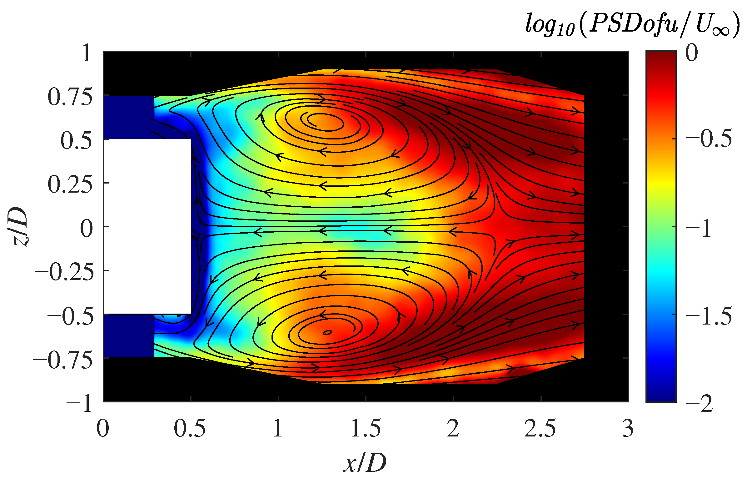
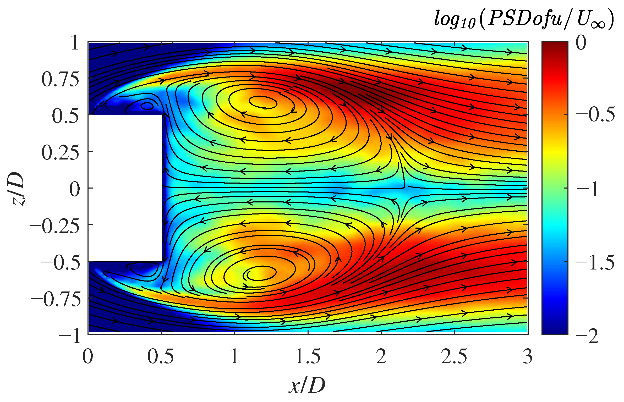
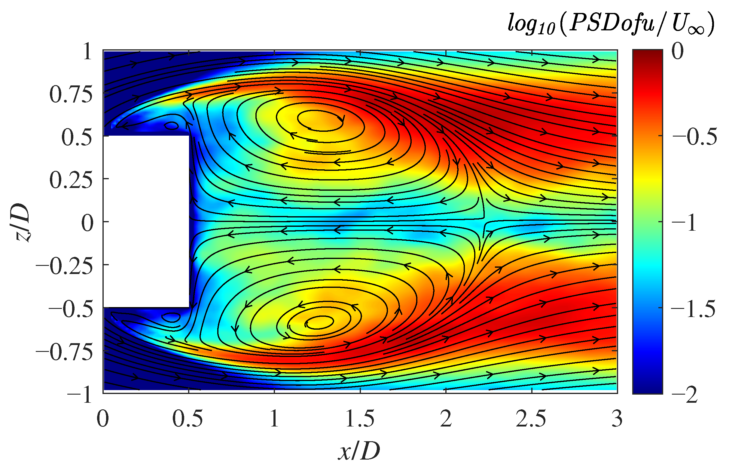
Figure 42, Figure 43 and Figure 44 show the PSD distributions of the x-direction velocity component u at St = 0.143, corresponding to the PIV measurement data, the simulation using default parameters, and the simulation using tuned parameters, respectively. PSD values are expressed in a common logarithm.
Although the PSD values along the center axis of the cylinder in the two simulation cases are very small, the PIV measurement data show slightly higher PSD values near the end of the recirculation bubble. Despite this difference, both the simulation cases and the PIV measurement data indicate significant fluctuations near the outer edge of the recirculation bubble, and the overall distribution patterns are similar. This suggests that the two simulation cases qualitatively capture the high-frequency velocity fluctuations caused by the helical vortex structures identified by Berger et al. However, a quantitative comparison of the high PSD distribution at the outer edge of the recirculation bubble reveals that the PSD values in the two simulation cases are lower than those in the PIV measurement data. This indicates that the simulations underestimate the influence of the helical vortex structures and the resulting velocity fluctuations compared to the PIV measurements. Furthermore, no significant quantitative improvement is observed because of parameter tuning.
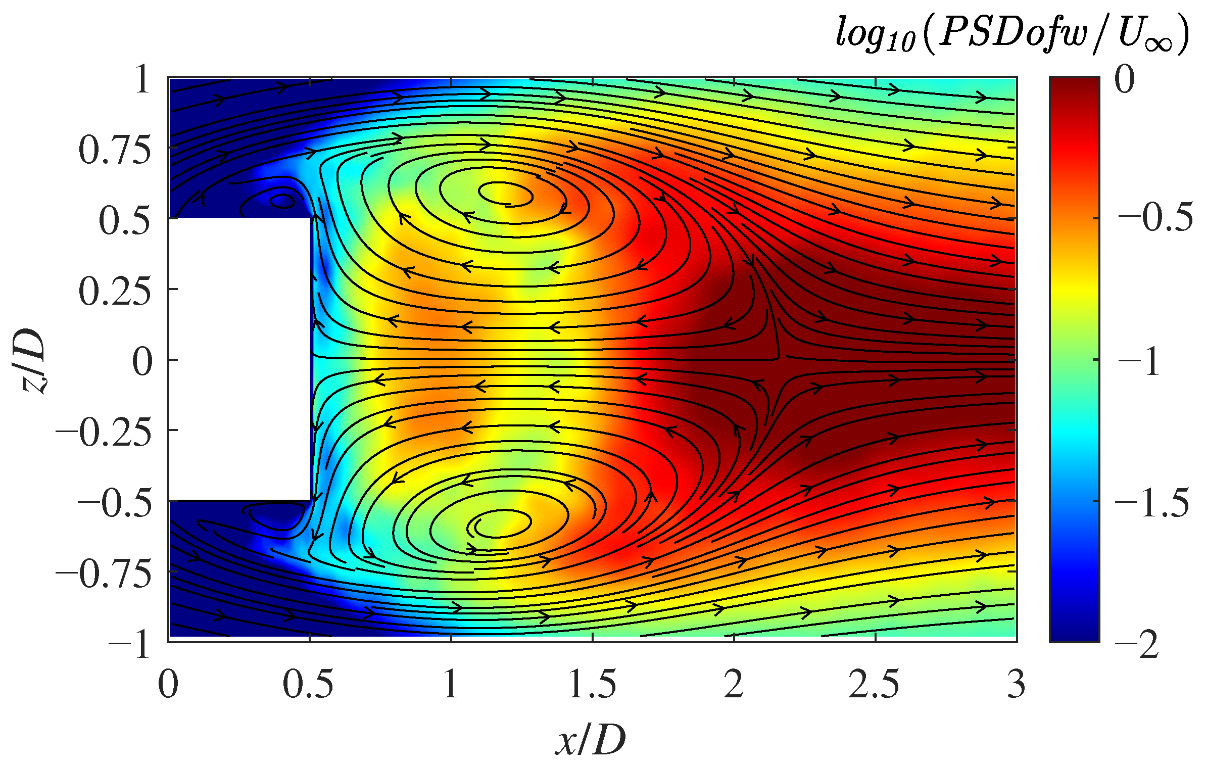
Figure 45, Figure 46 and Figure 47 show the PSD distributions of the z-direction velocity component w for the PIV measurement data, the simulation using default parameters, and the simulation using tuned parameters, respectively.
The PSD is concentrated near the stagnation point downstream of the recirculation bubble, with high values also observed near the back surface of the cylinder ( x / D = 1.0 ) . These qualitative features are consistent between the simulations and the PIV measurements, indicating that the simulations qualitatively capture the velocity fluctuations of the velocity component w well. However, as with the velocity component u, quantitative comparisons reveal clear differences between the PIV measurements and the simulations. The PSD distribution near the rear surface of the cylinder is significantly smaller in both simulation cases compared to the PIV data. Additionally, the region downstream of the recirculation bubble where the PSD exceeds 1.0 is narrower in the simulations than in the PIV measurements. Therefore, like the velocity component u, the simulations tend to underestimate the velocity fluctuations at S t 0.14 for the velocity component w. This tendency did not improve significantly even with parameter tuning.

3.8. Relationship Between Parameter Values and Simulation Results of Wake Velocity and Vorticity Components

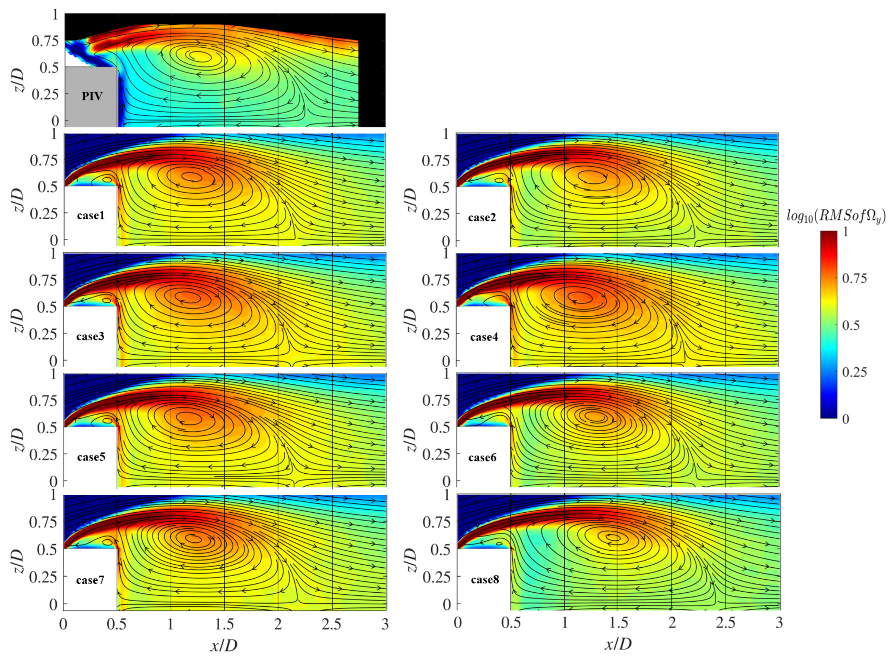
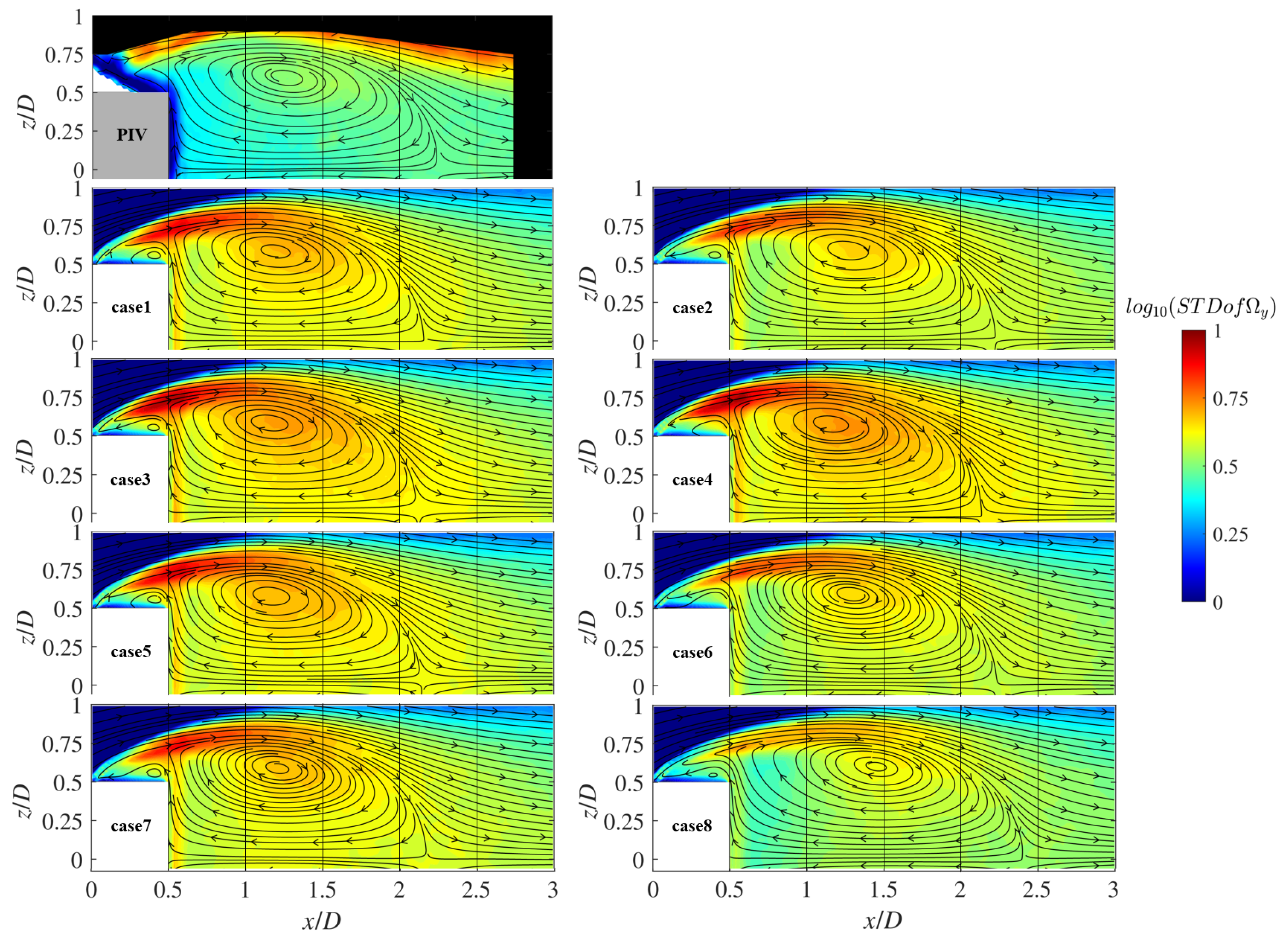
To verify the mechanism by which changes in parameter values affect simulation results, simulations were conducted under the following eight conditions with varying parameter values, and the vorticity component Ω y of the vorticity tensor was extracted and compared with PIV measurement results. The wake flow of a cylinder changes due to the separation shear layer generated at the leading edge of the cylinder and the disturbance of the separation shear layer caused by the Kelvin-Helmholtz instability. Therefore, by comparing the parameter values with the vorticity and vorticity fluctuations in the region around the leading edge of the cylinder and downstream of it, it is possible to understand the mechanism. The parameter values for each simulation case are shown in the Table 3 below. The simulation conditions, except for parameter values, are the same as those shown in Section 2.2.

3.8.1. Comparison of the Root Mean Square (RMS) of the Vorticity Component Ω y

Figure 48 shows a comparison of the RMS of the vorticity component Ω y in the PIV measurement and simulations in the wake region of the cylinder on the x-z plane through the center axis of the cylinder. Streamlines showing the time-averaged velocity are also shown. The PIV measurement result shows missing data near the leading edge, but all eight simulation results show strong vorticity caused by separation at the leading edge of the cylinder. These vorticities move downstream along the flow and gradually decrease. In both C b 1 and C d e s cases, it was shown that the high-vorticity region around x / D = 0.5 is thicker when the parameter values are smaller and becomes slightly thinner as the parameter values increase. The vorticity distribution near the rear surface of the cylinder is larger in cases with smaller parameter values and tends to decrease as the parameters increase. In addition, a notable difference is observed in the length of the high-vorticity region distributed along the separated shear layer and its downstream extension between changes in C b 1 and C d e s . Although varying C b 1 does not result in a clear difference, increasing the value of C d e s clearly extends the high-vorticity region farther downstream. Near the centers of the twin vortices that form the recirculation bubble, there exists a region where the vorticity generated by the leading edge separation diffuses. The vorticity distribution in this region does not show a strong sensitivity to changes in C b 1 values, but is significantly affected by changes in C d e s , showing a decreasing trend in vorticity as C d e s increases.

3.8.2. Comparison of the Standard Deviation (STD) of the Vorticity Component Ω y

Figure 49 shows a comparison of the STD of the vorticity component Ω y in the PIV measurement and simulations in the wake region of the cylinder on the x-z plane through the center axis of the cylinder. As in Figure 48, streamlines representing the time-averaged velocity components are also shown. In the region near the leading edge of the cylinder, where the separated shear layer exists, no distinct distribution is observed in the PIV measurements. However, the eight simulation cases exhibit strong vorticity fluctuations in this region. In particular, strong distributions appear near the separated share layer. Similarly to the results of the RMS of the vorticity component, variations in C d e s had a greater effect on the value of the vorticity variation than variations in C b 1 . Although changes in C b 1 did not show significant effects, an increase in C d e s led to reduced vorticity fluctuations in the separated shear layer region, near the centers of the twin vortices, and in the vicinity of the rear surface of the cylinder.

3.8.3. Relationship Between Parameter Tuning and Improvement in Time-Averaged Velocity Distribution

This section discusses the relationship between changes in parameter values due to tuning and the enlargement of the recirculation bubble. Figure 50 compares the time-averaged x-direction velocity u / U on the center axis of the cylinder, using PIV measurement data and the eight simulation cases corresponding to the parameters setting listed in Table 3. The results show that the velocity distribution is strongly dependent on the value of C d e s . As C d e s increases, the size of the recirculation bubble expands and the velocity gradient on the upstream side of the recirculation bubble ( 0.5 < x / D < 1.5 ) becomes more gradual. Additionally, both the position where the minimum velocity occurs and the minimum velocity value shift downstream and decrease, respectively, as C d e s increases.
An increase in C d e s corresponds to an increase in the vortex size treated as the turbulent viscosity coefficient in the SGS model. Furthermore, the turbulent viscosity coefficient within the computational domain is found to be higher than that obtained using the default parameters. Consequently, some of the vortex motions that were explicitly simulated under the default parameter setting are now treated as turbulent viscosity. As a result, the motion of small-scale vortices is suppressed compared to the simulation using the default parameters. As shown in Figure 48 and Figure 49, this leads to suppressed vorticity fluctuations in the separated shear layer near the cylinder’s leading edge, and an extension of the high-vorticity region downstream. As a result, the diffusion of the separated shear layer is suppressed and the recirculation bubble extends farther downstream compared to the case using the default parameters. This mechanism is considered to have brought both the size of the recirculation bubble and the time-averaged velocity distribution closer to the PIV data, thereby improving the simulation accuracy.

3.8.4. Relationship Between Parameter Tuning and Frequency Analysis Results

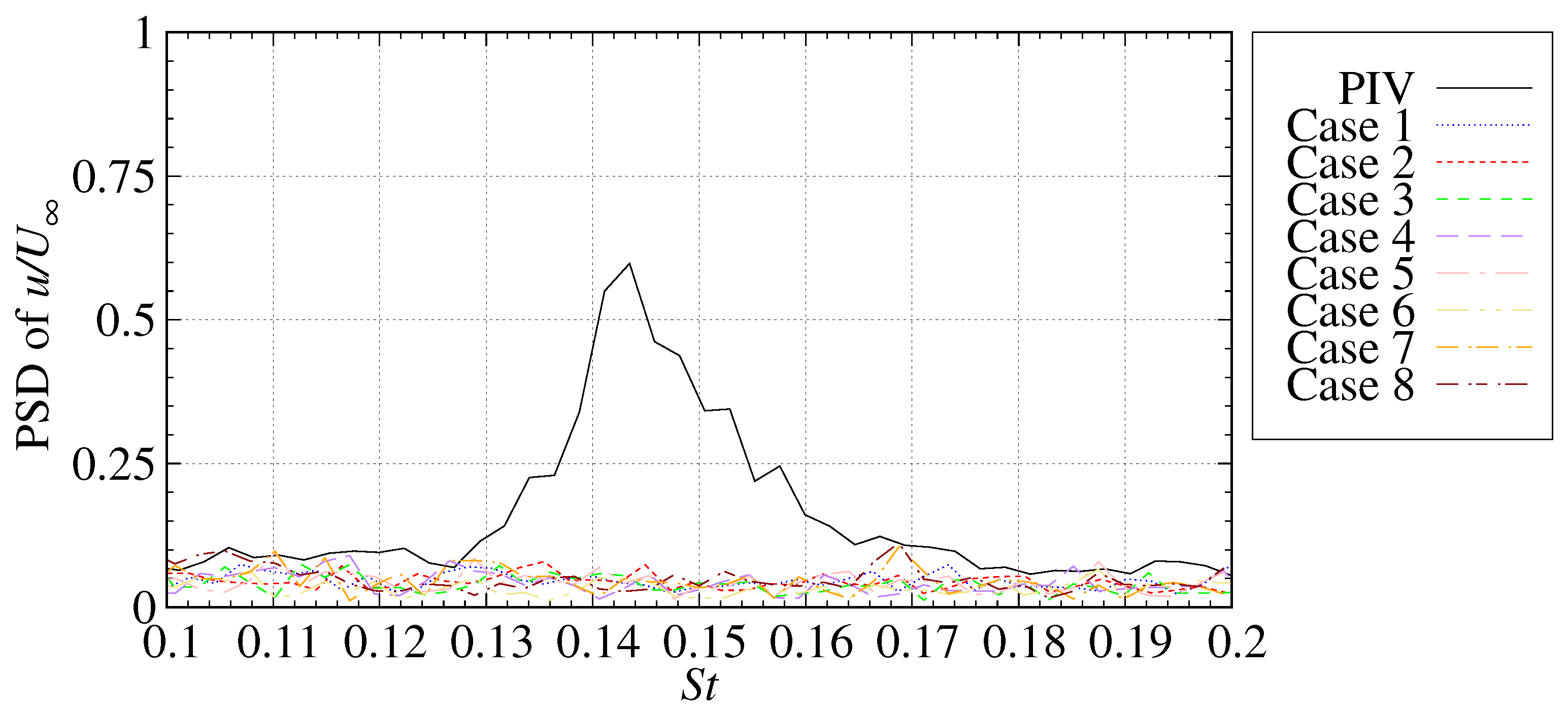
To examine the relationship between changes in parameter values and frequency variations in the cylinder wake, the PSD of the velocity components u and w was calculated using FFT at selected coordinates. Figure 51 and Figure 52 compare the PSD of u / U and w / U at ( x / D = 2.25 , z / D = 0.0 ), and Figure 53 and Figure 54 show the PSD at ( x / D = 2.0 , z / D = 0.65 ). The results from PIV measurements and eight simulation cases based on the parameter conditions listed in Table 3 are included. To clearly identify the positions and magnitudes of the PSD peak, the logarithmic axis was not used, and the horizontal axis was limited to the Strouhal number range of 0.1 0.2 . The coordinate point ( x / D = 2.25 , z / D = 0.0 ) corresponds to a stagnation point of wake in the PIV data, having a strong peak in the PSD of w / U . The coordinate point ( x / D = 2.0 , z / D = 0.65 ), located on the outer boundary of the recirculation bubble, has strong peaks in both u / U and w / U .
While the PIV data in Figure 51 captures a peak not seen in any simulation case, it appears at a slightly lower frequency than the other three figures, suggesting the need for further validation of this peak. Across all four figures, unlike the clear parameter-dependence observed in the time-averaged velocity distributions, no consistent trends in PSD distribution are seen among the eight simulation cases.
All cases showed significantly lower PSD values than the PIV data, with little variation among them. The Strouhal number at which the PSD peaks occur varies across cases, and no clear relationship is observed between parameter values and frequency characteristics. Additionally, case 3 and case 6, where C b 1 and C d e s were set significantly lower than default values, show different peak frequencies depending on coordinate location and velocity component. And then, Case 5 and case 8, where C b 1 and C d e s were set to their highest values, respectively, both show a few PSD peaks at S t 0.13 in Figure 54.
These variations in frequency characteristics are considered to result from complex effects of parameter-induced changes in wake vorticity. Decreasing parameter values increases vorticity fluctuations, destabilizing the separated shear layer, which likely introduces irregularity into the frequency components and causes variations in peak frequencies. Conversely, increasing parameter values stabilizes the shear layer, which may reduce the dominant frequency and enhance low-frequency fluctuations. The limited variation in PSD peak values with respect to parameter changes is likely due to the coarse spatial and temporal resolution of the simulation, as well as the large grid spacing. Under these conditions, the ability to capture short-time-scale flow fluctuations is limited, suggesting that changes in model parameters alone are insufficient to enhance high-frequency fluctuations. Therefore, under the simulation conditions applied in this study, it is considered that, in addition to parameter tuning, other techniques are necessary to improve the time variation characteristics of the flow.

3.8.5. Effect of Parameter Tuning in DES Through Comparison with LES and Consideration of Possible Improvements for Simulation Accuracy of DES

In addition, the LES results conducted by Kuwata et al. [18] were compared with the PIV measurements and the eight DDES cases to highlight the characteristics of simulation accuracy improvement achieved through parameter tuning using data assimilation with experimental results. This comparison evaluated the difference between the tuned DDES and the high-fidelity simulation, discussing potential improvements to the parameter tuning method. The condition of LES analysis is briefly described. This simulation method is called ‘Implicit LES (I-LES)’ because it does not use a subgrid-scale model. Kuwata et al. used the CFD solver called ‘LANS3D’ [27] based on the finite difference method for compressible fluids. A sixth-order accuracy compact scheme is used for spatial discretization, and a second-order backward difference scheme is used for time integration. The subiterations in each time step were calculated using the LUSGS method. The time step size was normalized to 0.0005 with respect to the cylinder diameter and sound speed. Reynolds number of the freestream was set to R e = 4.0 × 10 4 and the Mach number was set to M a = 0.2 . Although the Reynolds number is somewhat lower compared to the experiments and the DDES simulations, the flow studied in this research exhibits a low Reynolds number dependence on Reynolds numbers of the order of 10 4 . Therefore, it is appropriate to use the result of this LES as a comparison. The number of grid points was 351 in the radial direction, 201 in the azimuthal direction, and 751 in the flow direction. The simulation cost of the referenced LES is more than 100 times higher than that of DDES in this study due to the time step size and the number of grid points. Details of the LES simulation are described in [18].
Figure 55 compares the time-averaged velocity in the x-direction u / U along the cylinder center axis in the cylinder wake region, obtained by PIV measurements, eight DDES cases, and LES by Kuwata et al.
Focusing on the region farther downstream from the rear surface of the cylinder ( x / D > 1.5 ), the PIV and LES are same distribution, and the DDES case with tuned parameters shows a velocity distribution close to them. Therefore, it can be said that, in this region, parameter tuning improved the accuracy of the DDES simulation and the DDES simulation reproduced the high-fidelity simulation.
However, in the region near the rear surface of the cylinder, a notable difference is observed between the PIV measurements and LES results. Among the DDES cases, the case using the default parameters (case1) shows a distribution closer to LES than the case using tuned parameters (case2) that resemble the PIV data. Furthermore, the case in which C d e s and C b 1 are set to values smaller than the default values (case3 and case6) showed the distribution to be more like LES. In this study, data assimilation was performed using PIV measurement data as observations and the parameters were tuned so that the DDES results were closer to the PIV measurements. As a result, in the region near the rear surface of the cylinder, where the difference between LES and PIV is pronounced, the difference from LES is considered to be greater than in the case with default parameters. Since data assimilation improves simulations to reproduce the specific observation data used, it should be noted that, as in this study, there may be cases where the difference from high-fidelity simulations, such as LES, becomes larger in part of the computational domain.
The results of the eight DDES cases suggest that reproducing LES results requires using smaller parameter values near the cylinder rear surface and larger values farther downstream. For example, dividing the domain based on distance from the cylinder and assigning different parameter values to each region could enable more accurate tuning than the current method using uniform values throughout the domain.

4. Conclusions

This study examined the effectiveness of parameter tuning through data assimilation using wind tunnel experimental data to improve the simulation accuracy of large-scale separated flow around a cylinder facing the mainstream, using DDES. The assimilated data consisted of two-dimensional velocity fields in the wake measured by PIV, and the tuned parameters were C d e s and C b 1 . The velocity data was extracted from the simulation points corresponding to the coordinates of the PIV measurements used as observations, and the data assimilation was performed using only this data set. This approach significantly reduced the computational time required for data assimilation.
The parameter tuning resulted in a decrease in C b 1 and an increase in C d e s compared to the default values. Comparisons of turbulent viscosity and Reynolds stress indicated increased turbulent viscosity in the wake region, along with increased Reynolds stress.
Time-averaged velocity comparisons showed expansion of the recirculation bubble, and the simulation results grew closer to the PIV measurements. This result suggests the effect of parameter tuning of DES models to improve simulation accuracy of the size of the recirculation bubble and velocity distribution in the wake flow. In contrast, FFT analysis of unsteady velocity revealed that the frequency component generating the PSD peak in the recirculation bubble shifted toward lower frequencies after tuning, increasing the discrepancy with PIV data. The magnitude of the peak PSD remained largely unchanged.
Analysis of vorticity distributions indicated that increases in C b 1 and C d e s suppressed vorticity fluctuations in the separated shear layer near the cylinder’s leading edge. This suppression reduced shear layer diffusion, causing the recirculation bubble enclosed by the layer to extend farther downstream compared to the default case. As a result, the size of the recirculation bubble matched the PIV data more closely. However, the effect of changing parameter values on the wake flow fluctuations was not significant, especially the magnitude of the PSD peaks, which did not improve with parameter tuning. Therefore, under the simulation conditions of this study, improving both the time-averaged and time-dependent characteristics of the flow requires not only parameter tuning but also additional measures.
Comparison with LES results showed that the case with the smallest C b 1 and C d e s values best matched LES results in the flow field near the rear surface of the cylinder, while the result of the DDES cases with tuned values of the parameters best matched LES in the flow field far from the cylinder. These results suggest the possibility of the values of the optimal parameter for the simulation to vary depending on the simulation domain in turbulent flow simulation using DES.

Author Contributions

Conceptualization, K.N. and S.O.; Methodology, K.N.; Validation, K.N. and S.O.; Investigation, K.N.; Writing—original draft, K.N.; Writing—review and editing, S.O.; Supervision, S.O.; Project administration, S.O.; funding acquisition, S.O. All authors have read and agreed to the published version of the manuscript.

Funding

This study was supported by JSPS KAKENHI Grant number 21H04586.

Acknowledgments

This study was implemented using the Hokkaido University High-Performance Intercloud at the Information Initiative Center, Hokkaido University, Sapporo, Japan, and AFI-NITY at the Advanced Fluid Information Research Center, Institute of Fluid Science, Tohoku University, Sendai, Japan. We would like to express our gratitude to them. The CFD code “UTcart” used in this study was provided through the kind support of Yoshiharu Tamaki and Taro Imamura of the University of Tokyo. Sincere gratitude is expressed to both for their generous assistance.

Conflicts of Interest

The authors declare no conflicts of interest.

References

  1. Asada, K.; Kawai, S. Large-eddy simulation of airfoil flow near stall condition at Reynolds number 2.1 × 10⁶. Phys. Fluids 2018, 30, 085103-1–085103-22. [Google Scholar] [CrossRef]
  2. Rumsey, C.L.; Slotnick, J.P. Overview and Summary of the Second AIAA High Lift Prediction Workshop. In Proceedings of the AIAA Aerospace Sciences Meeting, National Harbor, MD, USA, 13–17 January 2014. AIAA paper 2014-0747. [Google Scholar]
  3. Sawada, E.; Aoyama, T.; Hamamoto, S.; Matsushima, K.; Imamura, T.; Yoshimoto, M.; Ueno, Y.; Nakakita, K.; Murayama, M. 6th Aerodynamics Prediction Challenge (APC-6). In Proceedings of the Fluid Dynamics Conference/Aerospace Numerical Simulation Symposium 2020 Online, Online, 28–30 September 2020. JAXA-SP-20-005. [Google Scholar]
  4. Strelets, M. Detached eddy simulation of massively separated flows. In Proceedings of the 39th Aerospace Sciences Meeting and Exhibit, Reno, Nevada, 8–11 January 2001. AIAA 2001-0879. [Google Scholar]
  5. Imamura, T.; Tamaki, Y. Unsteady Flow Simulation around Two-wheel Main Landing Gear based on Compressible Navier-Stokes Solver with Immersed Boundary Method. In Proceedings of the AIAA AVIATION 2020 FORUM, Virtual Event, 8 June 2020. AIAA 2020-2579. [Google Scholar]
  6. Ohmichi, Y.; Kobayashi, K.; Kanazaki, M. Numerical investigation of wake structures of an atmospheric entry capsule by modal analysis. Phys. Fluids 2019, 31, 074105-1-12. [Google Scholar] [CrossRef]
  7. Caruelle, B.; Ducros, F. Detached-Eddy Simulations of Attached and Detached Boundary Layers. Int. J. Comput. Fluid Dyn. 2003, 17, 433–451. [Google Scholar] [CrossRef]
  8. Spalart, P.R.; Deck, S.; Shur, M.L.; Squires, K.D.; Strelets, M.K.; Travin, A. A new version of detached-eddy simulation, resistant to ambiguous grid densities. Theor. Comput. Fluid Dyn. 2006, 20, 181–195. [Google Scholar] [CrossRef]
  9. Shur, M.L.; Spalart, P.R.; Strelets, M.K.; Travin, A.K. A hybrid RANS-LES approach with delayed-DES and wall-modelled LES capabilities. Int. J. Heat Fluid Flow 2008, 29, 1638–1649. [Google Scholar] [CrossRef]
  10. Kato, H.; Ishiko, K.; Yoshizawa, A. Optimization of Parameter Values in the Turbulence Model Aided by Data Assimilation. AIAA J. 2016, 54, 1512–1523. [Google Scholar] [CrossRef]
  11. Nakamura, M.; Ozawa, Y.; Nonomura, T. Low-grid-resolution-RANS-based Data Assimilation of Time Averaged Separated Flow Obtained by LES. Int. J. Comput. Fluid Dyn. 2022, 36, 167–185. [Google Scholar] [CrossRef]
  12. Berger, E.; Scholz, D.; Schumm, M. Coherent Vortex Structures in the Wake of a Sphere and a Circular Disk at Rest and Under Forced Vibrations. J. Fluids Struct. 1990, 4, 231–257. [Google Scholar] [CrossRef]
  13. Yang, J.; Liu, M.; Wu, G.; Zhong, W.; Zhang, X. Numerical Study on coherent structure behind a circular disk. J. Fluids Struct. 2014, 51, 172–188. [Google Scholar] [CrossRef]
  14. Camarri, S.; Salvetti, M.V.; Koobus, B.; Dervieux, A. Large-Eddy Simulation of a Bluff-Body Flow on Unstructured Grids. Int. J. Numer. Methods Fluids 2002, 40, 1431–1460. [Google Scholar] [CrossRef]
  15. Tiras, F.X.; Gorobets, A.; Oliva, A. Turbulent Flow around a Square Cylinder at Reynolds Number 22,000: A DNS Study. Comput. Fluids 2015, 123, 87–98. [Google Scholar] [CrossRef]
  16. Ito, S.; Furukawa, M.; Yamada, K.; Manabe, K. Applying Ensemble Kalman Filter to Transonic Flows Through a Two-Dimensional Turbine Cascade. J. Fluids Eng. 2021, 143, 121113. [Google Scholar] [CrossRef]
  17. Okuizumi, H.; Sawada, H.; Nagaike, H.; Konishi, Y.; Obayashi, S. Introduction of 1-m MSBS in Tohoku University, New Device for Aerodynamics Measurements of the Sports Equipment. In Proceedings of the 12th Conference of the International Sports Engineering Association (Proceeding Paper), Brisbane, QLD, Australia, 26–29 March 2018; Volume 2. [Google Scholar]
  18. Kuwata, M.; Abe, Y.; Sho, Y.; Nonomura, T.; Sawada, H.; Yakeno, A.; Asai, K.; Obayashi, S. Flow Characteristics around Extremely Low Fineness-Ratio Circular Cylinders. Phys. Rev. Fluids 2021, 6, 1–14. [Google Scholar] [CrossRef]
  19. Spalart, P.A.; Allmaras, S. One-Equation Turbulence Model for Aerodynamic Flows. In Proceedings of the 30th Aerospace Sciences Meeting and Exhibit, Reno, Nevada, 6–9 January 1992. AIAA-92-0439. [Google Scholar]
  20. Tamaki, Y.; Imamura, T. Turbulent Flow Simulations of the NASA Common Research Model Using the Immersed Boundary Method with a Wall Function. In Proceedings of the 35th AIAA Applied Aerodynamics Conference, Denver, CO, USA, 5–9 June 2017. AIAA 2017-4235. [Google Scholar]
  21. Mavriplis, D.J. Revisiting the Least-Squares Procedure for Gradient Reconstruction on Unstructured. In Proceedings of the 16th AIAA Computational Fluid Dynamics Conference, Orlando, FL, USA, 23–26 June 2003. AIAA 2003-3986. [Google Scholar]
  22. van Leer, B. Towards the ultimate conservative difference scheme. V. A second-order sequel to Godunov’s method. J. Comput. Phys. 1979, 32, 101–136. [Google Scholar] [CrossRef]
  23. Shima, E.; Kitamura, K. On New Simple Low-Dissipation Scheme of AUSM-Family for akk Speeds. In Proceedings of the 47th AIAA Aerospace Sciences Meeting Including the New Horizons Forum and Aerospace Exposition, Orlando, FL, USA, 5–8 January 2009. AIAA-2009-136. [Google Scholar]
  24. Yoon, S.; Jameson, A. Lower-upper Symmetric-Gauss-Seidel method for the Euler and Navier-Stokes equations. AIAA J. 1988, 26, 1025–1026. [Google Scholar] [CrossRef]
  25. Tippett, M.K.; Anderson, J.L.; Bishop, C.H.; Hamill, T.M.; Whitaker, J.S. Ensemble Square Root Filters. Mon. Weather. Rev. 2003, 131, 1485–1490. [Google Scholar] [CrossRef]
  26. Evensen, G. Sequential Data Assimilation with a Nonlinear Quasi-Geostrophic Model using Monte Carlo Methods to Forecast Error Statistics. J. Geophys. Res. 1994, 99, 10143–10162. [Google Scholar] [CrossRef]
  27. Fujii, K. Developing an Accurate and Efficient Method for Compressible Flow Simulation—An Example of CFD in Aeronautics. In Proceedings of the 5th International Conference on Numerical Ship Hydrodynamics, Washington, DC, USA, 24–28 September 1990. [Google Scholar]
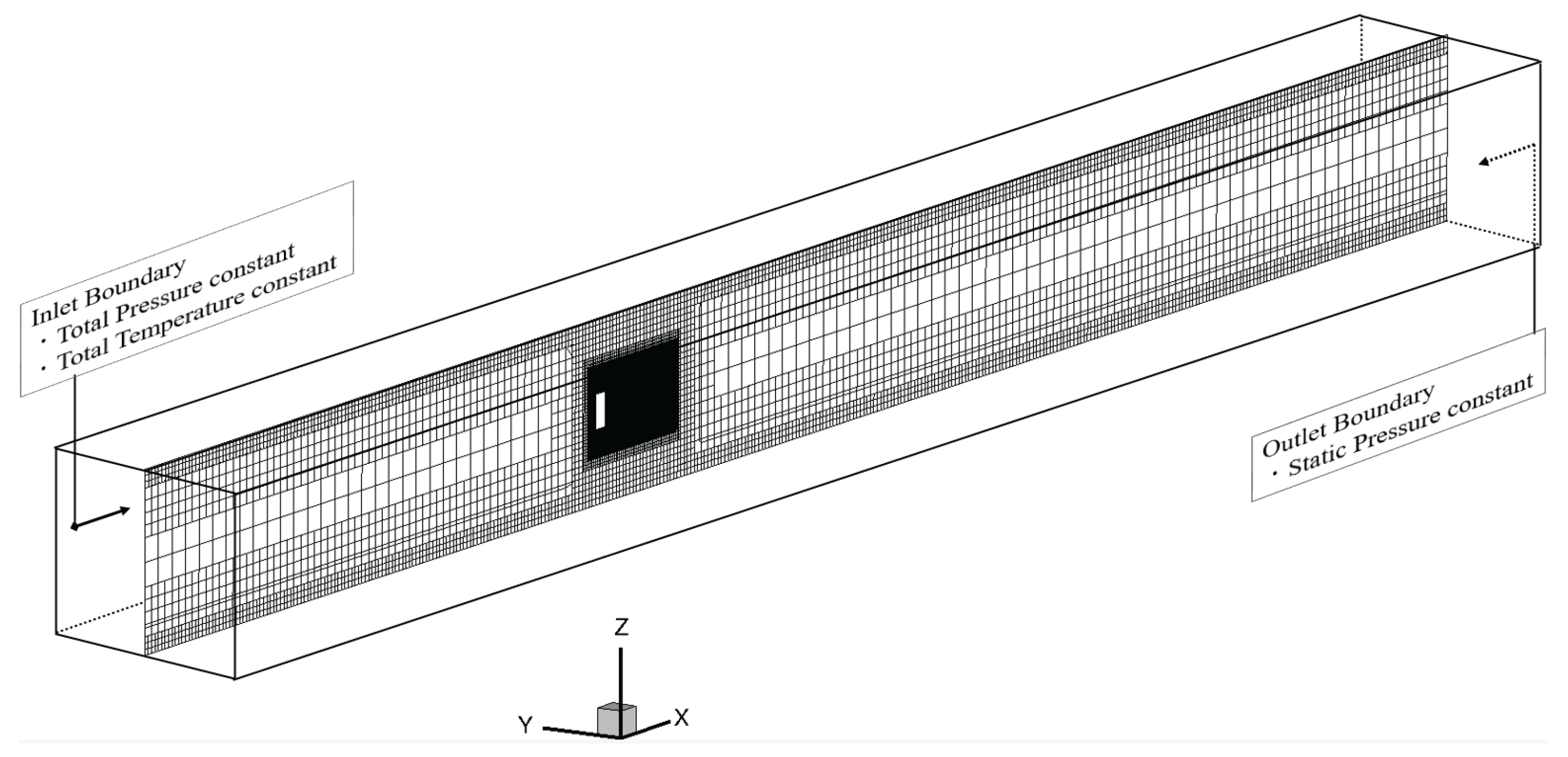
Figure 1. Boundary condition and grid outline.
Aerospace 12 00736 g001
Figure 2. Grid condition around a cylinder.
Aerospace 12 00736 g002
Figure 3. Outline of the velocity distribution on x-z plane through the center axis of the cylinder.
Aerospace 12 00736 g003
Figure 4. Locations of observation data.
Aerospace 12 00736 g004
Figure 5. Tuning history of the mean of the C b 1 values of the ensemble members.
Aerospace 12 00736 g005
Figure 6. Tuning history of the variance of the C b 1 values of the ensemble members.
Aerospace 12 00736 g006
Figure 7. Tuning history of the mean of the C d e s values of the ensemble members.
Aerospace 12 00736 g007
Figure 8. Tuning history of the variance of the C d e s values of the ensemble members.
Aerospace 12 00736 g008
Figure 9. Turbulent viscosity coefficient μ t in x-z plane along the center axis of the cylinder with default parameters.
Aerospace 12 00736 g009
Figure 10. Turbulent viscosity coefficient μ t in x-z plane along the center axis of the cylinder with tuned parameters.
Aerospace 12 00736 g010
Figure 11. Comparison of turbulent viscosity coefficient μ t on the center axis of the cylinder.
Aerospace 12 00736 g011
Figure 12. Comparison of turbulent viscosity coefficient μ t on the z-axis at x/D = 0.25.
Aerospace 12 00736 g012
Figure 13. Comparison of turbulent viscosity coefficient μ t on the z-axis at x/D = 1.5.
Aerospace 12 00736 g013
Figure 14. Reynolds stress component in x-z plane on the center axis of the cylinder obtained by PIV measurement.
Aerospace 12 00736 g014
Figure 15. Reynolds stress component in x-z plane on the center axis of the cylinder with default parameters.
Aerospace 12 00736 g015
Figure 16. Reynolds stress component in x-z plane on the center axis of the cylinder with tuned parameters.
Aerospace 12 00736 g016
Figure 17. x-direction velocity distribution in x-z plane on the center axis of the cylinder obtained by PIV measurement.
Aerospace 12 00736 g017
Figure 18. x-direction velocity distribution in x-z plane on the center axis of the cylinder with default parameters.
Aerospace 12 00736 g018
Figure 19. x-direction velocity distribution in x-z plane on the center axis of the cylinder with tuned parameters.
Aerospace 12 00736 g019
Figure 20. Comparison of X-direction velocity distribution on the center axis of the cylinder.
Aerospace 12 00736 g020
Figure 21. Comparison of X-direction velocity distribution along the z axis at the streamwise location x / D = 0.75 .
Aerospace 12 00736 g021
Figure 22. Comparison of X-direction velocity distribution along the z axis at the streamwise location x / D = 1.5 .
Aerospace 12 00736 g022
Figure 23. Comparison of X-direction velocity distribution along the z axis at the streamwise location x / D = 2.25 .
Aerospace 12 00736 g023
Figure 24. Standard Deviation of x-direction velocity u obtained by PIV measurement.
Aerospace 12 00736 g024
Figure 25. Standard Deviation of x-direction velocity u obtained by simulation using default parameters.
Aerospace 12 00736 g025
Figure 26. Standard Deviation of x-direction velocity u obtained by simulation using tuned parameters.
Aerospace 12 00736 g026
Figure 27. Standard Deviation of z-direction velocity w obtained by PIV measurement.
Aerospace 12 00736 g027
Figure 28. Standard Deviation of z-direction velocity w obtained by simulation using default parameters.
Aerospace 12 00736 g028
Figure 29. Standard Deviation of z-direction velocity w obtained by simulation using tuned parameters.
Aerospace 12 00736 g029
Figure 30. Comparison of Standard Deviation of x-direction velocity u along the z axis at the x / D = 0.75 .
Aerospace 12 00736 g030
Figure 31. Comparison of Standard Deviation of x-direction velocity u along the z axis at the x / D = 1.5 .
Aerospace 12 00736 g031
Figure 32. Comparison of Standard Deviation of x-direction velocity u along the z axis at the x / D = 2.25 .
Aerospace 12 00736 g032
Figure 33. Comparison of Standard Deviation of z-direction velocity w along the z axis at the x / D = 0.75 .
Aerospace 12 00736 g033
Figure 34. Comparison of Standard Deviation of z-direction velocity w along the z axis at the x / D = 1.5 .
Aerospace 12 00736 g034
Figure 35. Comparison of Standard Deviation of z-direction velocity w along the z axis at the x / D = 2.25 .
Aerospace 12 00736 g035
Figure 36. Comparison of PSD of x-direction velocity u at the point 1.
Aerospace 12 00736 g036
Figure 37. Comparison of PSD of z-direction velocity w at the point 1.
Aerospace 12 00736 g037
Figure 38. Comparison of PSD of x-direction velocity u at the point 2.
Aerospace 12 00736 g038
Figure 39. Comparison of PSD of z-direction velocity w at the point 2.
Aerospace 12 00736 g039
Figure 40. Comparison of PSD of x-direction velocity u at the point 3.
Aerospace 12 00736 g040
Figure 41. Comparison of PSD of z-direction velocity w at the point 3.
Aerospace 12 00736 g041
Figure 42. PSD of x-direction velocity u at S t = 0.143 obtained by PIV measurement.
Aerospace 12 00736 g042
Figure 43. PSD of x-direction velocity u at S t = 0.143 obtained by simulation using default parameters.
Aerospace 12 00736 g043
Figure 44. PSD of x-direction velocity u at S t = 0.143 obtained by simulation using tuned parameters.
Aerospace 12 00736 g044
Figure 45. PSD of z-direction velocity w at S t = 0.143 obtained by PIV measurement.
Aerospace 12 00736 g045
Figure 46. PSD of z-direction velocity w at S t = 0.143 obtained by simulation using default parameters.
Aerospace 12 00736 g046
Figure 47. PSD of z-direction velocity w at S t = 0.143 obtained by simulation using tuned parameters.
Aerospace 12 00736 g047
Figure 48. Comparisons of RMS of vorticity component Ω y between PIV measurement result and simulation results from eight cases of DDES.
Aerospace 12 00736 g048
Figure 49. Comparisons of STD of vorticity component Ω y between PIV measurement result and simulation results from eight cases of DDES.
Aerospace 12 00736 g049
Figure 50. Comparisons of time-averaged velocity distribution u / U on the center axis of the cylinder between PIV measurement result and simulation results from eight cases of DDES.
Aerospace 12 00736 g050
Figure 51. Comparisons of PSD of x-direction velocity u / U at (x/D = 2.25, z/D = 0.0) between PIV measurement result and simulation results from eight cases of DDES.
Aerospace 12 00736 g051
Figure 52. Comparisons of PSD of z-direction velocity w / U at (x/D = 2.25, z/D = 0.0) between PIV measurement result and simulation results from eight cases of DDES.
Aerospace 12 00736 g052
Figure 53. Comparisons of PSD of x-direction velocity u / U at (x/D = 2.0, z/D = −0.65) between PIV measurement result and simulation results from eight cases of DDES.
Aerospace 12 00736 g053
Figure 54. Comparisons of PSD of z-direction velocity w / U at (x/D = 2.0, z/D = −0.65) between PIV measurement result and simulation results from eight cases of DDES..
Aerospace 12 00736 g054
Figure 55. Comparisons of time-averaged velocity distribution on the center axis of the cylinder between PIV measurement result, simulation results from eight cases of DDES and simulation result from I-LES by Kuwara et al.
Aerospace 12 00736 g055
Table 1. Comparisons of default and tuned parameters for C b 1 and C d e s .
ParameterDefaultTunedRelative Error
C b 1 0.13550.118512.5%
C d e s 0.650.829227.5%
Table 2. Location and value of the minimum x-direction velocity u m i n / U along the center axis of the cylinder.
LocationValue
PIV (Kuwata)1.40−0.471
DDES-Default1.23−0.483
DDES-Tuned1.35−0.468
Table 3. Parameter values set for the eight cases of DDES simulations.
C b 1 C des
Case 10.1355 (default)0.65 (default)
Case 20.1083 (tuned)0.8619 (tuned)
Case 30.060.65
Case 40.10830.65
Case 50.20.65
Case 60.13550.4
Case 70.13550.8619
Case 80.13551.0
Disclaimer/Publisher’s Note: The statements, opinions and data contained in all publications are solely those of the individual author(s) and contributor(s) and not of MDPI and/or the editor(s). MDPI and/or the editor(s) disclaim responsibility for any injury to people or property resulting from any ideas, methods, instructions or products referred to in the content.