
A Review of Simulations and Machine Learning Approaches for Flow Separation Analysis


Abstract
1. Introduction
2. Mechanisms and Impacts of Flow Separation
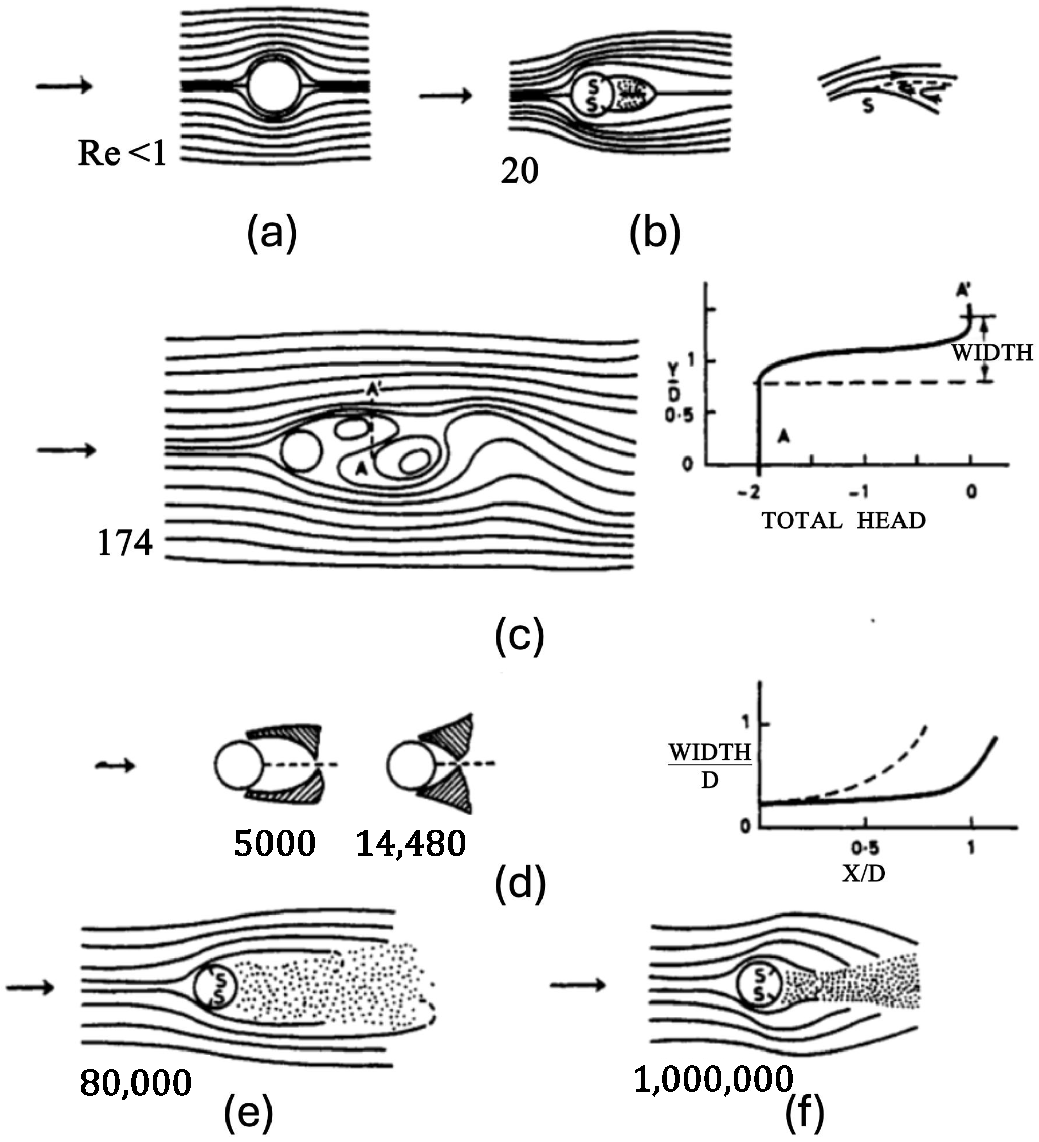
2.1. 2D Flow Separation
2.2. 3D Flow Separation

2.3. Discussion
3. Simulations for Flow Separation
3.1. RANS

| Reference | Geometry | Key Parameters | Methods | Key Findings | Limitations |
|---|---|---|---|---|---|
| Langtry et al. [30] | S809 airfoil (21% thickness) | Re = , AoA = 1°– 20°. FSTI = 0.2% | SST with transition model | Improved prediction of separation bubbles and torque; good prediction of lift/drag at moderate AoA | Struggles with massively separated flows; requires empirical correlations |
| Wolgemuth & Walters [31] | NACA0012 airfoil at varying AoA | Re = – , AoA = 0°– 20°, Tu = 0.01–2% | Transition-sensitive | Good prediction of separation bubbles | Overpredicts stall angles at low Re; requires unsteady solvers for convergence |
| Furst et al. [32] | Flat plate; two NACA0012 airfoils in tandem; VKI turbine blade | Re = , Tu = 0.3–9.43% | Algebraic model () with intermittency vs. model | Both predict bypass/natural transition; is better for separated flows | Grid dependency near walls; algebraic model struggles with 3D effects |
| Menter et al. [33] | Flat plates (T3 series); Pak-B turbine blader; T106 cascade; V103 compressor | Re = – , Tu = 0.03–8% | One equation intermittency () model coupled with SST | Galilean invariant; captures the separation bubbles and reattachment | Limited calibration for crossflow transition; requires fine grids for separation bubbles |
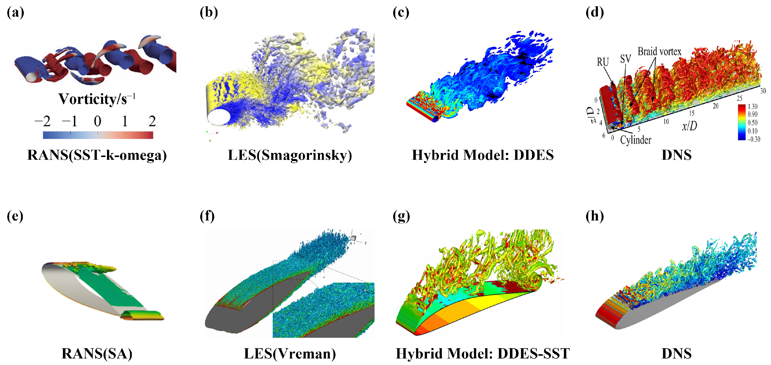
3.2. LES
3.3. DNS
3.4. Hybrid Modeling Techniques
3.4.1. Hybrid CFD Methods
3.4.2. Incorporated High-Order Methods in CFD Simulations
3.4.3. ROM
3.5. LBM
3.6. Further Discussion
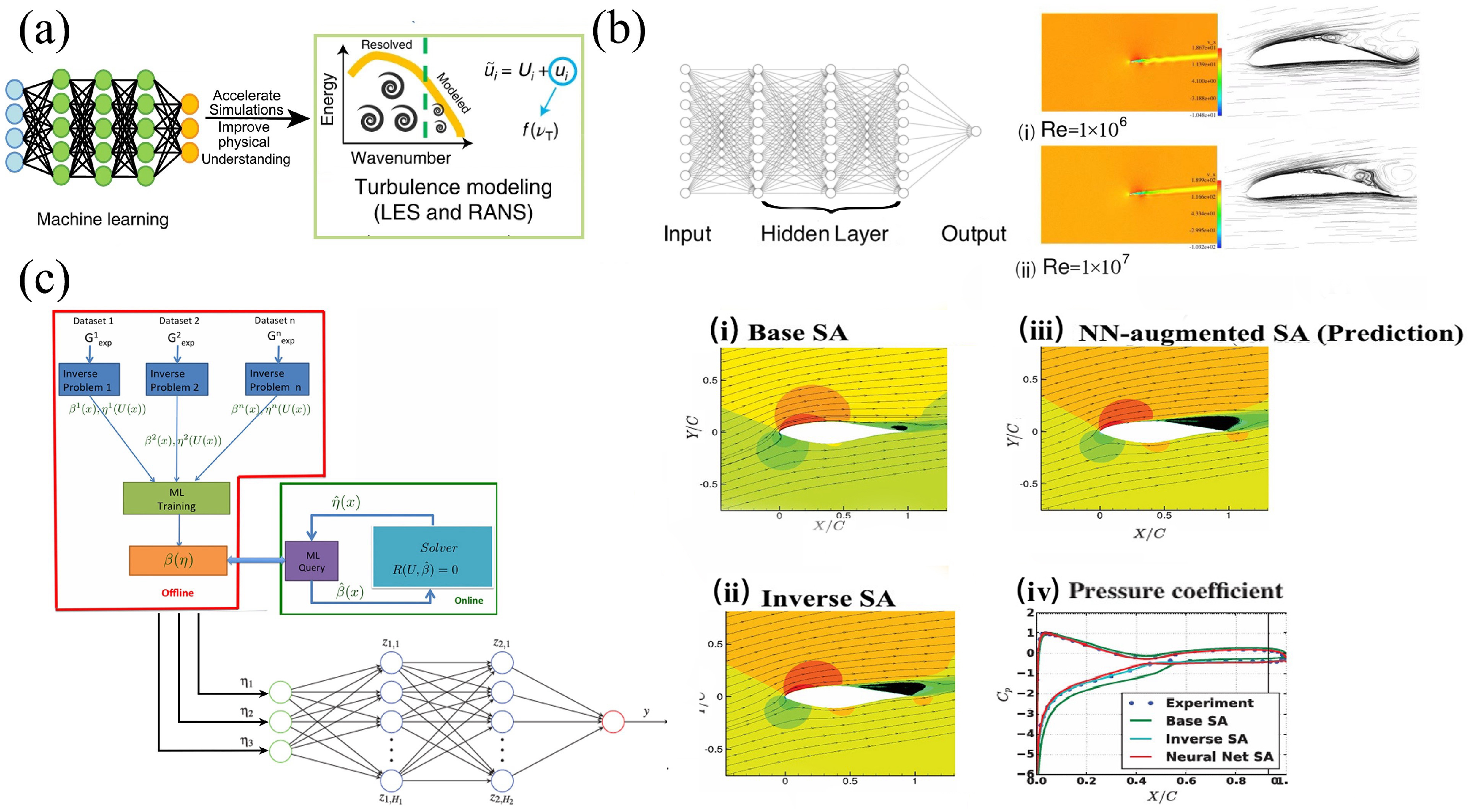
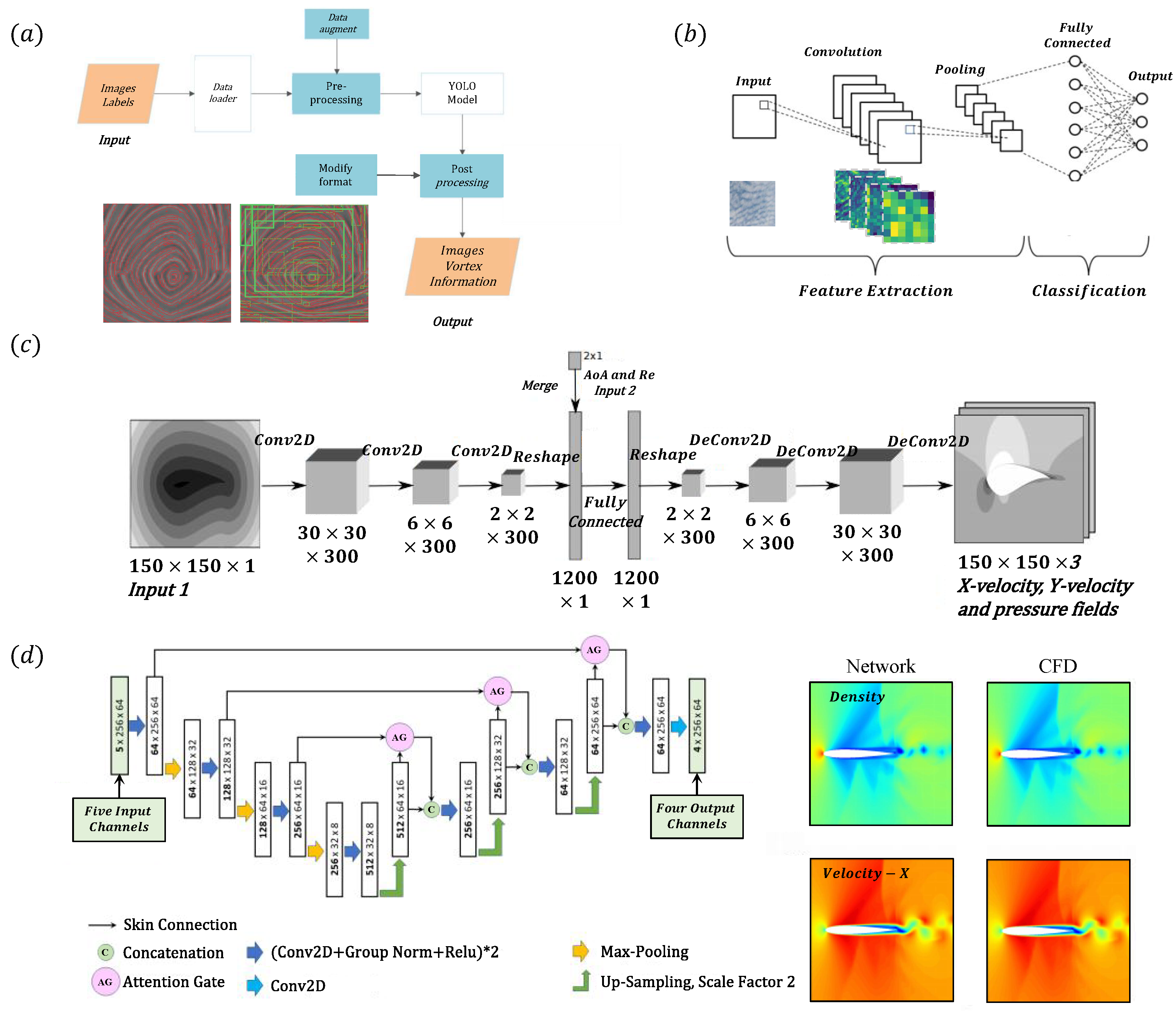
4. ML for Flow Separation
4.1. ML Enhancement of Turbulent Modelling Closure
4.2. ML-Enhanced ROMs
4.3. CNNs
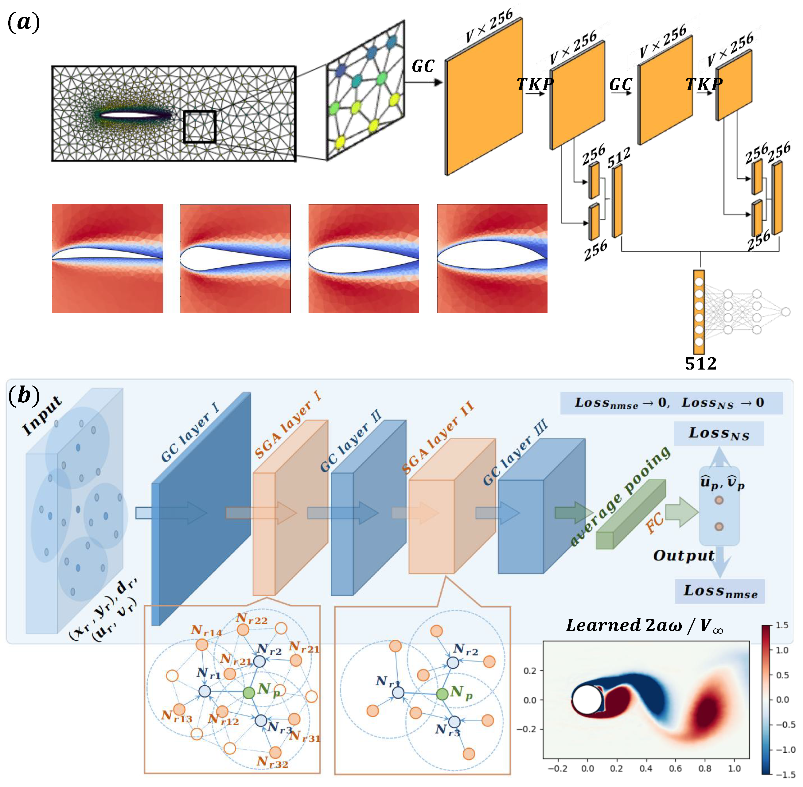
4.4. GNNs
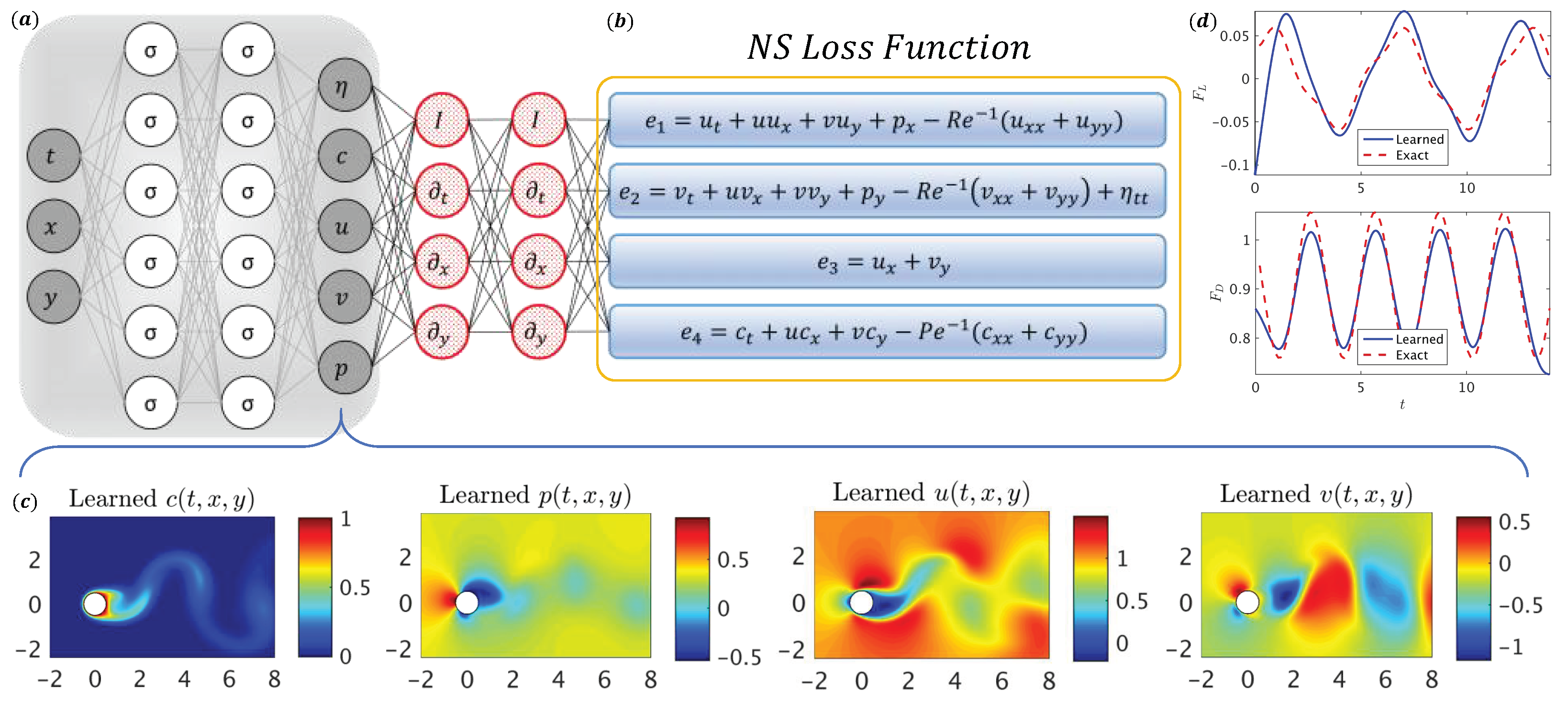
4.5. PINNs
4.6. Data Assimilation Enhanced ML
5. Discussions and Future Trends
Author Contributions
Funding
Data Availability Statement
Acknowledgments
Conflicts of Interest
References
- Roshko, A. Perspectives on Bluff Body Aerodynamics. J. Wind. Eng. Ind. Aerodyn. 1992, 49, 79–100. [Google Scholar] [CrossRef]
- Rizzi, A.; Luckring, M.J. Historical Development and Use of CFD for Separated Flow Simulations Relevant to Military Aircraft. Aerosp. Sci. Technol. 2021, 117, 106940. [Google Scholar] [CrossRef]
- Gursul, I.; Wang, Z. Flow Control of Tip/Edge Vortices. AIAA J. 2018, 56, 1731–1749. [Google Scholar] [CrossRef]
- Li, Y.; Chang, J.; Kong, C.; Bao, W. Recent Progress of Machine Learning in Flow Modeling and Active Flow Control. Chin. J. Aeronaut. 2022, 35, 14–44. [Google Scholar] [CrossRef]
- Sun, X.; Xu, Y.; Huang, D. Numerical Simulation and Research on Improving Aerodynamic Performance of Vertical Axis Wind Turbine by Co-flow Jet. J. Renew. Sustain. Energy 2019, 11, 013303. [Google Scholar] [CrossRef]
- Heinz, S. The Potential of Machine Learning Methods for Separated Turbulent Flow Simulations: Classical Versus Dynamic Methods. Fluids 2024, 9, 278. [Google Scholar] [CrossRef]
- Mokhtarpoor, R.; Heinz, S.; Stoellinger, M. Dynamic Unified RANS-LES Simulations of High Re Separated Flows. Phys. Fluids 2016, 28, 095101. [Google Scholar] [CrossRef]
- Zhao, Z.; Wang, J.; Gong, Y.; Xu, H. Large Eddy Simulation of Flow and Separation Bubbles Around a Circular Cylinder from Sub-critical to Super-critical Reynolds Numbers. J. Mar. Sci. Appl. 2023, 22, 219–231. [Google Scholar] [CrossRef]
- Ohlsson, J.; Schlatter, P.; Fischer, F.P.; Henningson, S.D. Direct Numerical Simulation of Separated Flow in a Three-dimensional Diffuser. J. Fluid Mech. 2010, 650, 307–318. [Google Scholar] [CrossRef]
- Brunton, S.L.; Noack, B.R.; Koumoutsakos, P. Machine Learning for Fluid Mechanics. Annu. Rev. Fluid Mech. 2020, 52, 477–508. [Google Scholar] [CrossRef]
- Jin, X.; Cai, S.; Li, H.; Karniadakis, G.E. NSFnets (Navier-Stokes flow nets): Physics-Informed Neural Networks for the Incompressible Navier-Stokes Equations. J. Comput. Phys. 2021, 426, 109951. [Google Scholar] [CrossRef]
- Greenblatt, D.; Wygnanski, J.I. The Control of Fow Separation by Periodic Excitation. Prog. Aerosp. Sci. 2000, 36, 487–545. [Google Scholar] [CrossRef]
- Chang, P.K. Introduction to the Problems of Flow Separation. In Separation of Flow; Pergamon Press: Oxford, UK, 1970; pp. 3–35. [Google Scholar]
- Schlichting, H.; Gersten, K. Boundary Layer Theory. In Fundamentals of Boundary—Layer Theory; Springer: Berlin, Germany, 2017; pp. 29–49. [Google Scholar]
- Bezzola, A. Optimal Bass Reflex Loudspeaker Port Design. In Proceedings of the COMSOL Conference 2019, Boston, MA, USA, 2–4 October 2019. [Google Scholar]
- Van Dyke, M. An Album of Fluid Motion; The Parabolic Press: Stanford, CA, USA, 1982. [Google Scholar]
- Wikipedia Contributors. Flow Separation. Available online: https://en.wikipedia.org/wiki/Flow_separation (accessed on 3 March 2025).
- Pope, S.B. Wall Flows. In Turbulent Flows; Cambridge University Press: Cambridge, UK, 2000; pp. 264–332. [Google Scholar]
- Graham, M.; Li, J. Vortex Shedding and Induced Forces in Unsteady Flow. Aeronaut. J. 2024, 128, 2149–2190. [Google Scholar] [CrossRef]
- Leibovich, S.; Luckring, J.M. The Structure of Vortex Breakdown. Annu. Rev. Fluid Mech. 1978, 10, 221–246. [Google Scholar] [CrossRef]
- Wang, S.; He, G.; Liu, T. Estimating lift from wake velocity data in flapping flight. J. Fluid Mech. 2019, 868, 501–537. [Google Scholar] [CrossRef]
- Li, J.; Zhao, X.; Graham, M. Vortex force maps for three-dimensional unsteady flows with application to a delta wing. J. Fluid Mech. 2020, 900, A36. [Google Scholar] [CrossRef]
- Simpson, R.L. Junction Flows. Annu. Rev. Fluid Mech. 2001, 33, 415–443. [Google Scholar] [CrossRef]
- Délery, J. Separation in Three-Dimensional Flow: Critical Points, Separation Lines, and Vortices. Onera—The French Aerospace Lab. 2011. Available online: https://www.onera.fr/sites/default/files/ressources_documentaires/cours-exposes-conf/onera-3d-separation-jean-delery-2011-1a.pdf (accessed on 2 January 2025).
- Durbin, P.A. Some Recent Developments in Turbulence Closure Modeling. Annu. Rev. 2018, 50, 77–103. [Google Scholar] [CrossRef]
- Chaouat, B. The State of the Art of Hybrid RANS/LES Modeling for the Simulation of Turbulent Flows. Flow Turbul. Combust 2017, 99, 279–327. [Google Scholar] [CrossRef]
- Duraisamy, K.; Iaccarino, G.; Xiao, H. Turbulence Modeling in the Age of Data. Annu. Rev. Fluid Mech. 2019, 51, 357–377. [Google Scholar] [CrossRef]
- Peng, S.H.; Eliasson, P. Examination of the Shear Stress Transport Assumption with a Low-Reynolds Number k–ω Model for Aerodynamic Flows. In Proceedings of the 37th AIAA Fluid Dynamics Conference and Exhibit, Miami, FL, USA, 25–28 June 2007. AIAA 2007-3864. [Google Scholar]
- Liu, Y.; Li, P.; Jiang, K. Comparative Assessment of Transitional Turbulence Models for Airfoil Aerodynamics in the Low Reynolds Number Range. J. Wind. Eng. Ind. Aerodyn. 2021, 217, 104726. [Google Scholar] [CrossRef]
- Langtry, R.B.; Gola, J.; Menter, F.R. A One-Equation Local Correlation-Based Transition Model. In Proceedings of the 44th AIAA Aerospace Sciences Meeting and Exhibit, Reno, NV, USA, 9–12 January 2006. AIAA 2006-395. [Google Scholar]
- Wolgemuth, N.M.; Walters, D.K. CFD Prediction of Boundary Layer Transition And Separation on an Airfoil at Varying Angle of Attack. In Proceedings of the EDSM2007 5th Joint ASME/JSME Fluids Engineering Conference, San Diego, CA, USA, 30 July–2 August 2007. FEDSM2007-37111. [Google Scholar]
- Fürst, J.; Příhoda, J.; Straka, P. Numerical Simulation of Transitional Flows. Computing 2013, 95, S163–S182. [Google Scholar] [CrossRef]
- Menter, F.R.; Smirnov, P.E.; Liu, T.; Avancha, R. A One-Equation Local Correlation-Based Transition Model. Flow Turbul. Combust 2015, 95, 583–619. [Google Scholar] [CrossRef]
- Xia, X.; You, Z.; Wang, Z. The three types of turbulence models and stability numerical simulation studies for cylindrical flow. Hydro-Sci. Eng. 2024, 5, 84–94. [Google Scholar]
- Lysenko, D.A.; Ertesvåg, I.S.; Rian, K.E. Large-Eddy Simulation of the Flow Over a Circular Cylinder at Reynolds Number 3900 Using the OpenFOAM Toolbox. Flow Turbul. Combust 2012, 89, 491–518. [Google Scholar] [CrossRef]
- Zhang, D.; Cadel, D.R.; Paterson, E.G.; Lowe, K.T. Hybrid RANS/LES Turbulence Model Applied to a Transitional Unsteady Boundary Layer on Wind Turbine Airfoil. Fluids 2019, 4, 128. [Google Scholar] [CrossRef]
- Li, J.; Wang, B.; Qiu, X.; Wu, J.; Zhou, Q.; Fu, S.; Liu, Y. Three-dimensional vortex dynamics and transitional flow induced by a circular cylinder placed near a plane wall with small gap ratios. J. Fluid Mech. 2022, 953, A2. [Google Scholar] [CrossRef]
- Guo, H.; Li, G.; Zou, Z. Numerical Simulation of the Flow around NACA0018 Airfoil at High Incidences by Using RANS and DES Methods. J. Mar. Sci. Eng. 2022, 10, 847. [Google Scholar] [CrossRef]
- Arias-Ramírez, W.; Oberoi, N.; Larsson, J. Multifidelity Approach to Sensitivity Estimation in Large-Eddy Simulation. AIAA J. 2023, 61, 3485–3495. [Google Scholar] [CrossRef]
- Sa, J.H.; Park, S.H.; Kim, C.J.; Park, J.K. Low-Reynolds number flow computation for eppler 387 wing using hybrid DES/transition model. J. Mech. Sci. Technol. 2015, 29, 1837–1847. [Google Scholar] [CrossRef]
- Beck, A.D.; Bolemann, T.; Flad, D.; Frank, H.; Gassner, G.J.; Hindenlang, F.; Munz, C. High-order discontinuous Galerkin spectral element methods for transitional and turbulent flow simulations. J. Int. J. Numer. Meth. Fluids. 2014, 76, 522–548. [Google Scholar] [CrossRef]
- Zhao, M. A Review of Recent Studies on the Control of Vortex-induced Vibration of Circular Cylinders. Ocean. Eng. 2023, 285, 115389. [Google Scholar] [CrossRef]
- Liang, Z.; Wang, J.; Jiang, B.; Zhou, H.; Yang, W.; Ling, J. Large-Eddy Simulation of Flow Separation Control in Low-Speed Diffuser Cascade with Splitter Blades. Processes 2023, 11, 3249. [Google Scholar] [CrossRef]
- Piomelli, U.; Balaras, E. Wall-layer Models for Large-Eddy Simulations. Annu. Rev. Fluid Mech. 2002, 34, 349–374. [Google Scholar] [CrossRef]
- Meng, T.; Li, X.; Zhou, L.; Zhu, H.; Li, J.; Ji, L. Large Eddy Simulation and Combined Control of Corner Separation in a Compressor Cascade. Phys. Fluids 2022, 34, 075113. [Google Scholar] [CrossRef]
- Kawai, S.; Larsson, J. Wall-modeling in Large Eddy Simulation: Length Scales, Grid Resolution, and Accuracy. Phys. Fluids 2012, 24, 015105. [Google Scholar] [CrossRef]
- Malik, R.M.; Uzun, A. DNS of Accelerating and Decelerating Turbulent Flow. In Proceedings of the AIAA Aviation 2020 Forum, Virtual, 19 August 2020. [Google Scholar]
- Jones, L.E.; Sandberg, R.D.; Sandham, N.D. Direct Numerical Simulations of Forced and Unforced Separation Bubbles on an Airfoil at Incidence. J. Fluid Mech. 2008, 602, 175–207. [Google Scholar] [CrossRef]
- Shahab, M.F.; Omidyeganeh, M.; Pinelli, A. DNS of Separated Low-Re Flow Around a Cambered Aerofoil. In Direct and Large-Eddy Simulation XI; Springer: Berlin/Heidelberg, Germany, 2019; pp. 373–380. [Google Scholar]
- Spalart, R.P.; Watmuff, H.J. Experimental and Numerical Study of a Turbulent Boundary Layer with Pressure Gradients. J. Fluid Mech. 1993, 249, 337–371. [Google Scholar] [CrossRef]
- Wu, X.; Moin, P. Direct Numerical Simulation of Turbulence in A Nominally Zero-pressure-gradient Flat-plate Boundary Layer. J. Fluid Mech. 2009, 630, 5–41. [Google Scholar] [CrossRef]
- Coleman, G.N.; Sandberg, R.D. A Primer on Direct Numerical Simulation of Turbulence- Methods, Procedures and Guidelines; Technical Report AFM-09/01b; University of Southampton: Southampton, UK, 2010. [Google Scholar]
- Zhang, W.; Samtaney, R. Assessment of Spanwise Domain Size Effect on the Transitional Flow Past an Airfoil. Comput. Fluids 2016, 124, 39–53. [Google Scholar] [CrossRef]
- Cummings, M.R.; Squires, K.; Spalart, P. Multidisciplinary Applications of Detached-Eddy Simulation to Separated Flows at High Reynolds Numbers. In Proceedings of the 2004 Users Group Conference, Williamsburg, VA, USA, 7–11 June 2004; pp. 103–111. [Google Scholar]
- Spalart, P.R.; Deck, S.; Shur, M.L.; Squires, K.D.; Strelets, M.K.; Travin, A. A New Version of Detached-eddy Simulation, Resistant to Ambiguous Grid Densities. Theor. Comput. Fluid Dyn. 2006, 20, 181–195. [Google Scholar] [CrossRef]
- Menter, F.R. Stress-Blended Eddy Simulation (SBES)—A New Paradigm in Hybrid RANS-LES Modeling. In Proceedings of the 6th Symposium on Hybrid RANS-LES Methods, Strasbourg, France, 20–21 November 2018; pp. 27–37. [Google Scholar]
- Menter, F.R.; Egorov, Y. The Scale-Adaptive Simulation Method for Unsteady Turbulent Flow Predictions. Part 1: Theory and Model Description. Flow Turbul. Combust 2010, 85, 113–138. [Google Scholar] [CrossRef]
- Moller, F.M.; Tucker, P.G.; Wang, Z.; Morsbach, C.; Bergmann, M. On the Prediction of Separation-Induced Transition by Coupling Delayed Detached-Eddy Simulation with γ-Transition Model. In Proceedings of the 15th European Conference on Turbomachinery Fluid Dynamics & Thermodynamics, Budapest, Hungary, 24–28 April 2023. [Google Scholar]
- Sandrin, S.; Mazzei, L.; Soghe, R.D.; Fontaneto, F. Computational Fluid Dynamics Prediction of External Thermal Loads on Film-Cooled Gas Turbine Vanes: A Validation of Reynolds-Averaged Navier–Stokes Transition Models and Scale-Resolving Simulations for the VKI LS-94 Test Case. Fluids 2024, 9, 91. [Google Scholar] [CrossRef]
- Rezaeiha, A.; Montazeri, H.; Blocken, B. CFD Analysis of Dynamic Stall on Vertical Axis Wind Turbines using Scale Adaptive Simulation (SAS): Comparison against URANS and Hybrid RANS/ LES. Energy Convers. Manag. 2019, 196, 1281–1298. [Google Scholar] [CrossRef]
- Weihing, P.; Letzgus, T.; Kramer, E. Development of Alternative Shielding Functions for Detached-Eddy Simulations. In Progress in Hybrid RANS-LES Modelling, Notes on Numerical Fluid Mechanics and Multidisciplinary Design; Hoarau, Y., Peng, S.H., Schwamborn, D., Revell, A., Mockett, C., Eds.; Springer: Cham, Switzerland, 2019; pp. 109–118. [Google Scholar]
- Haering, W.S.; Oliver, A.T.; Moser, D.R. Active Model Split Hybrid RANS/LES. Phys. Rev. Fluids 2022, 7, 014603. [Google Scholar] [CrossRef]
- Wang, Z.J.; Fidkowski, K.; Abgrall, R.; Bassi, F.; Caraeni, D.; Cary, A.; Deconinck, H.; Hartmann, R.; Hillewaert, K.; Huynh, H.T.; et al. High-order CFD Methods: Current Status and Perspective. Int. J. Numer. Methods Fluids 2013, 72, 811–845. [Google Scholar] [CrossRef]
- Wang, S.; Dong, Y.; Deng, X. High-Order Simulation of Aeronautical Separated Flows with a Reynold Stress Model. J. Aircr. 2018, 55, 1177–1190. [Google Scholar] [CrossRef]
- Krank, B.; Kronbichler, M.; Wall, W.A. Wall Modeling via Function Enrichment Within a High-order DG Method for RANS Simulations of Incompressible flow. Int. J. Numer. Methods Fluids, 2024; accepted. [Google Scholar] [CrossRef]
- Ding, Q.; Zhao, M.; Xian, J.; Chen, Y.; Hao, S.; Cheng, C.; Li, X.; Liu, Z. Large Eddy Simulation Based on An Improved High-precision Interior Penalty Discontinuous Galerkin Method: Flow Past Cylinders and Airfoils. Acta Mech. 2024, 235, 6599–6623. [Google Scholar] [CrossRef]
- Brill, S.R.; Pal, P.; Ameen, M.; Xu, C.; Ihme, M. An Enrichment Wall Modeling Framework for Spectral Element Methods. Phys. Fluids 2024, 36, 125169. [Google Scholar] [CrossRef]
- Gassner, G.J.; Beck, A.D. On the Accuracy of High-order Discretizations for Underresolved Turbulence Simulations. Theor. Comput. Fluid Dyn. 2013, 27, 221–237. [Google Scholar] [CrossRef]
- Lucia, D.J.; Beran, P.S.; Silva, W.A. Reduced-order Modelling: New Approaches for Computational Physics. Prog. Aerosp. Sci. 2004, 40, 51–117. [Google Scholar] [CrossRef]
- Xu, Z.; Cao, N.Y.; Li, C.; Luo, Y.; Su, E.; Wang, W.; Tang, W.; Yao, Z.; Wang, Z.L.A. Digital Mapping of Surface Turbulence Status and Aerodynamic Stall on Wings of a Flying aircraft. Nat. Commun. 2023, 14, 2792. [Google Scholar] [CrossRef]
- Berkooz, G.; Holmes, P.; Lumley, J.L. The Proper Orthogonal Decomposition in the Analysis of Turbulent Flows. Annu. Rev. Fluid Mech. 1993, 25, 539–575. [Google Scholar] [CrossRef]
- Sajadmanesh, S.M.; Mojaddam, M.; Mohseni, A.; Nikparto, A. Numerical Identification of Separation Bubble in an Ultra-high-lift Turbine Cascade Using URANS Simulation and Proper Orthogonal Decomposition. Aerosp. Sci. Technol. 2019, 93, 105329. [Google Scholar] [CrossRef]
- Tong, F.; Sun, D.; Li, X. Direct Numerical Simulation of Impinging Shock Wave and Turbulent Boundary Layer Interaction over a Wavy-wall. Chin. J. Aeronaut. 2021, 34, 350–363. [Google Scholar] [CrossRef]
- Zhao, M.; Zhao, Y.; Liu, Z. Dynamic Mode Decomposition Analysis of Flow Characteristics of an Airfoil with Leading Edge Protuberances. Aerosp. Sci. Technol. 2020, 98, 105684. [Google Scholar] [CrossRef]
- Taira, K.; Hemati, M.S.; Brunton, S.L.; Sun, Y.; Duraisamy, K.; Bagheri, S.; Dawson, S.T.M.; Yeh, C. Modal Analysis of Fluid Flows: Applications and Outlook. AIAA J. 2020, 58, 998–1022. [Google Scholar] [CrossRef]
- Chen, S.; Doolen, G.D. Lattice Boltzmann Method for Fluid Flows. Annu. Rev. 1998, 30, 329–364. [Google Scholar] [CrossRef]
- Ribeiro, R.L.; Dantas, C.; Wolf, W. Intermittency of a Transitional Airfoil Flow with Laminar Separation Bubble Solved by the Lattice-Boltzmann Method. Aerosp. Sci. Technol. 2025, 158, 109907. [Google Scholar] [CrossRef]
- Premnath, K.N.; Pattison, M.J.; Banerjee, S. An Investigation of the Lattice Boltzmann Method for Large Eddy Simulation of Complex Turbulent Separated Flow. J. Fluids Eng. 2013, 135, 051401. [Google Scholar] [CrossRef]
- Zhu, Y.; Zhao, S.; Zhou, Y.; Liang, H.; Bian, X. An unstructured adaptive mesh refinement for steady flows based on physics-informed neural networks. arXiv 2024, arXiv:2411.19200. [Google Scholar]
- Wan, Z.; Zhang, W. A unified method of data assimilation and turbulence modeling for separated flows at high Reynolds numbers. Phys. Fluids 2023, 35, 025124. [Google Scholar]
- Xu, Z.; Maria, A.; Chelli, K.; Premare, T.D.; Bilbao, X.; Petit, C.; Zoumboulis-Airey, R.; Moulitsas, I.; Teschner, T.; Asif, S.; et al. Vortex and Core Detection using Computer Vision and Machine Learning Methods. Eur. J. Comput. Mech. 2023, 32, 467–494. [Google Scholar] [CrossRef]
- Hu, L.; Wang, W.; Xiang, Y.; Zhang, J. Flow Field Reconstructions with GANs Based on Radial Basis Functions. IEEE Trans. Aerosp. Electron. Syst. 2022, 58, 3460–3476. [Google Scholar] [CrossRef]
- Li, N.; Liu, Y.; Gong, G.; Zhao, L.; Yuan, H. A generative deep learning approach for real-time prediction of hypersonic vehicles in fluid-thermo-structural coupling fields. Aerosp. Sci. Technol. 2023, 139, 108398. [Google Scholar] [CrossRef]
- Guéniat, F.; Mathelin, L.; Hussaini, M.Y. A Statistical Learning Strategy for Closed-Loop Control of Fluid Flows. Theor. Comput. Fluid Dyn. 2016, 30, 497–510. [Google Scholar] [CrossRef]
- Zhu, L.; Zhang, W.; Kou, J.; Liu, Y. Machine Learning Methods for Turbulence Modeling in Subsonic Flows Around Airfoils. Phys. Fluids 2019, 31, 015105. [Google Scholar] [CrossRef]
- Vinuesa, R.; Brunton, S.L. Enhancing computational fluid dynamics with machine learning. Nat. Comput. Sci. 2022, 2, 358–366. [Google Scholar] [CrossRef]
- Areias, P.; Correia, R.; Melicio, R. Airfoil Analysis and Optimization Using a Petrov–Galerkin Finite Element and Machine Learning. Aerospace 2023, 10, 638. [Google Scholar] [CrossRef]
- Singh, A.P.; Medida, S.; Duraisamy, K. Machine-Learning-Augmented Predictive Modeling of Turbulent Separated Flows over Airfoils. AIAA J. 2017, 55, 2215–2227. [Google Scholar] [CrossRef]
- Ling, J.; Kurzawski, A.; Templeton, J. Reynolds Averaged Turbulence Modelling Using Deep Neural Networks with Embedded Invariance. J. Fluid Mech. 2016, 807, 155–166. [Google Scholar] [CrossRef]
- Zhang, B. Airfoil-based Convolutional Autoencoder and Long Short-term Memory Neural Network for Predicting Coherent Structures Evolution Around an Airfoil. Comput. Fluids 2023, 258, 105883. [Google Scholar] [CrossRef]
- Liu, Z.; Han, R.; Zhang, M.; Zhang, Y.; Zhou, H.; Wang, G.; Chen, G. An Enhanced Hybrid Deep Neural Network Reduced-order Model for Transonic Buffet Flow Prediction. Aerosp. Sci. Technol. 2022, 126, 107636. [Google Scholar] [CrossRef]
- Jia, X.; Li, C.; Ji, W.; Gong, C. A Hybrid Reduced-order Model Combing Deep Learning for Unsteady Flow. Phys. Fluids 2022, 34, 097112. [Google Scholar] [CrossRef]
- Phung, V.H.; Rhee, E.J. A High-Accuracy Model Average Ensemble of Convolutional Neural Networks for Classification of Cloud Image Patches on Small Datasets. Appl. Sci. 2019, 34, 4500. [Google Scholar] [CrossRef]
- Bhatnagar, S.; Afshar, Y.; Pan, S.; Duraisamy, K.; Kaushik, S. Prediction of Aerodynamic Flow Fields Using Convolutional Neural Networks. Comput. Mech. 2019, 64, 525–545. [Google Scholar] [CrossRef]
- Chen, L.; Thuerey, N. Deep learning-based predictive modeling of transonic flow over an airfoil. Phys. Fluids 2024, 36, 127106. [Google Scholar] [CrossRef]
- Han, R.; Wang, Y.; Zhang, Y.; Chen, G. A novel spatial-temporal prediction method for unsteady wake flows based on hybrid deep neural network. Phys. Fluids 2019, 31, 127101. [Google Scholar] [CrossRef]
- Sekar, V.; Jiang, Q.; Shu, C.; Khoo, B.C. Fast Flow Field Prediction over Airfoils Using Deep Learning Approach. Phys. Fluids 2019, 31, 057103. [Google Scholar] [CrossRef]
- Duru, C.; Alemdar, H.; Baran, O.U. A Deep Learning Approach for the Transonic Flow Field Predictions Around Airfoils. Comput. Fluids 2022, 236, 105312. [Google Scholar] [CrossRef]
- Lee, S.; You, D. Data-Driven Prediction of Unsteady Flow Over a Circular Cylinder Using Deep Learning. J. Fluid Mech. 2019, 879, 217–254. [Google Scholar] [CrossRef]
- Ogoke, F.; Meidani, K.; Hashemi, A.; Farimani, B. Graph Convolutional Networks Applied to Unstructured Flow Field Data. Mach. Learn. Sci. Technol. 2021, 2, 045020. [Google Scholar] [CrossRef]
- He, X.; Wang, Y.; Li, J. Flow Completion Network: Inferring the Fluid Dynamics from Incomplete Flow Information Using Graph Neural Networks. Phys. Fluids 2022, 34, 087114. [Google Scholar] [CrossRef]
- Massegur, D.; Da, R.A. Graph convolutional multi-mesh autoencoder for steady transonic aircraft aerodynamics. Mach. Learn. Sci. Technol. 2024, 5, 025006. [Google Scholar] [CrossRef]
- Hines, D.; Philipp, B. Graph neural networks for the prediction of aircraft surface pressure distributions. Aerosp. Sci. Technol. 2023, 137, 108268. [Google Scholar] [CrossRef]
- Yiren, S.; Alonso, J. Performance Evaluation of a Graph Neural Network-Augmented Multi-Fidelity Workflow for Predicting Aerodynamic Coefficients on Delta Wings at Low Speed. In Proceedings of the AIAA SCITECH 2025 Forum, Orlando, FL, USA, 6–10 January 2025; pp. 2025–2360. [Google Scholar]
- Raissi, M.; Wang, Z.; Triantafyllou, M.S.; Karniadakis, G.E. Deep learning of vortex-induced vibrations. J. Fluid Mech 2019, 861, 119–137. [Google Scholar] [CrossRef]
- Ren, Z.; Hu, P.; Su, H.; Zhang, F.; Yu, H. Physics-Informed Neural Networks for Transonic Flow Around a Cylinder with High Reynolds Number. Phys. Fluids 2024, 36, 036129. [Google Scholar] [CrossRef]
- Mons, V.; Chassaing, J.C.; Gomez, T.; Sagaut, P. Reconstruction of Unsteady Viscous Flows Using Data Assimilation Schemes. J. Comput. Phys. 2016, 316, 255–280. [Google Scholar] [CrossRef]
- Maulik, R.; Egele, R.; Raghavan, K.; Balaprakash, P. Quantifying Uncertainty for Deep Learning Based Forecasting and Flow-reconstruction Using Neural Architecture Search Ensembles. Phys. D 2023, 454, 133852. [Google Scholar] [CrossRef]


| Category | Method | Key Parameters | Advantages | Limitations |
|---|---|---|---|---|
| Traditional | RANS | NACA0012, NACA4415 Airfoil , [29] | Significantly reduced computational cost. | Unable to accurately capture transient turbulent structures; limited predictive capability for separated flows. |
| LES | NACA65-010, [43]; Blade NACA65 Airfoil, , [45] | Captures transient flow characteristics at high Re numbers, providing superior predictive capability for separated flows compared to RANS. | Significantly higher computational cost than RANS especially under conditions of high Re or complex geometries; requires high grid resolution near walls. | |
| DNS | NACA0012, NACA65(12)10 , [48] | Resolves all scales of turbulent structures, offering the highest accuracy. | Requires extremely high grid resolution and fine time step; computational cost increases exponentially with Re. | |
| Hybrid CFD | Circular cylinder, Airfoil, ; [55,59,60]; | Balances computational cost with accuracy, enabling simulations of high Re at complex geometries. | Low accuracy with strong interactions between turbulence scales; smooth transition between RANS and LES regions. | |
| High-Order | NACA0012 , [63] | High fidelity in resolving
separation dynamics and complex flow features. | Heavy dependence on turbulence modelling; high computational cost and time. | |
| ROM | Cascade, , [72]; NACA0012 Airfoil, , [74]; | Significant cost reduction due to essential flow physics preservation compared to traditional CFD methods. | Reliance on data quality and selected mode for accuracy. | |
| LBM | NACA0012 Airfoil , [77] | Parallel efficiency; suitable for complex geometries and multiphase. | Challenges in handling high Re; compressibility constraints; associated computational costs. | |
| Machine Learning | ML-Enhanced Turbulent Modelling | Airfoils, [87,88] [89] | Improved accuracy; limited training data; must deal with high Re. | Limited model generality; physical constraints and uncertainties; challenges in model interpretability; low adaptability. |
| ML-Enhanced ROMs | Cylinder and airfoils [90,91,92] | Improved accuracy with low computational cost. | Error accumulation; limited universality; extended training time; limited performance for high-Re turbulent flows. | |
| CNNs | Airfoils, Cylinder [94,95,96,97,98,99] | High accuracy; some generalization ability; reduce computational cost. | Limited by the quality and quantity of training data; difficulty in accurately predicting some complex flow phenomena such as small-scale vortical structures. | |
| GNNs | Cylinder, airfoils, aircraft, delta wings [100,101,102,103,104], , | Handle
unstructured data; improve accuracy; good generalization ability. | Low adaptability to complex geometries and flow conditions; greatly rely on data quality and quantity. | |
| PINNs | Cylinder [101,105,106] | High efficiency with low costs; integrate physical laws; efficient data utilization. | Challenges in high-Re turbulence and unsteady cases. | |
| Data Assimilation | Cylinder, [107] | Method innovation; relevance to practical applications. | Statistical dependence issues; computational efficiency and scalability. |
Disclaimer/Publisher’s Note: The statements, opinions and data contained in all publications are solely those of the individual author(s) and contributor(s) and not of MDPI and/or the editor(s). MDPI and/or the editor(s) disclaim responsibility for any injury to people or property resulting from any ideas, methods, instructions or products referred to in the content. |
© 2025 by the authors. Licensee MDPI, Basel, Switzerland. This article is an open access article distributed under the terms and conditions of the Creative Commons Attribution (CC BY) license (https://creativecommons.org/licenses/by/4.0/).
Share and Cite
Hao, X.; He, X.; Zhang, Z.; Li, J. A Review of Simulations and Machine Learning Approaches for Flow Separation Analysis. Aerospace 2025, 12, 238. https://doi.org/10.3390/aerospace12030238
Hao X, He X, Zhang Z, Li J. A Review of Simulations and Machine Learning Approaches for Flow Separation Analysis. Aerospace. 2025; 12(3):238. https://doi.org/10.3390/aerospace12030238
Chicago/Turabian StyleHao, Xueru, Xiaodong He, Zhan Zhang, and Juan Li. 2025. "A Review of Simulations and Machine Learning Approaches for Flow Separation Analysis" Aerospace 12, no. 3: 238. https://doi.org/10.3390/aerospace12030238
APA StyleHao, X., He, X., Zhang, Z., & Li, J. (2025). A Review of Simulations and Machine Learning Approaches for Flow Separation Analysis. Aerospace, 12(3), 238. https://doi.org/10.3390/aerospace12030238