Abstract
The tethered space net robot offers an effective solution for active space debris removal due to its large capture envelope. However, most existing studies overlook the evasive behavior of non-cooperative targets. To address this, we model an orbital pursuit–evasion game involving a tethered net and propose a game theory-based leader–follower tracking control strategy. In this framework, a virtual leader—defined as the geometric center of four followers—engages in a zero-sum game with the evader. An adaptive dynamic programming method is employed to handle input saturation and compute the Nash Equilibrium strategy. In the follower formation tracking phase, a synchronous distributed model predictive control approach is proposed to update all followers’ control simultaneously, ensuring accurate tracking while meeting safety constraints. The feasibility and stability of the proposed method are theoretically analyzed. Additionally, a body-fixed reference frame is introduced to reduce the capture angle. Simulation results show that the proposed strategy successfully captures the target and outperforms existing methods in both formation keeping and control efficiency.
1. Introduction
For on-orbit capture missions, flexible tethered space nets (TSNs) are highly effective for debris removal and non-cooperative target capture, providing a wide range and reduced precision requirements compared to traditional methods like robotic arms or harpoons [1,2]. To further enhance control over the position and configuration of the deployed net, recent advances have led to the development of maneuverable tethered space net robots (TSNRs), which integrate a deformable tethered net with four actively controlled spacecraft that coordinate their motion to adjust the net’s configuration [3,4]. While recent studies have extensively explored the formation control of the TSNR system, few have considered the potential evasive maneuvers of non-cooperative targets. However, when the target exhibits such autonomous behavior, existing formation tracking methods may compromise capture performance. The TSNR capture problem thus becomes an orbital pursuit–evasion game (OPEG) scenario, further complicated by the safety constraints caused by the tethered net.
The safety constraints in the TSNR system primarily revolve around maintaining appropriate inter-spacecraft distances [5]. As the four maneuvering spacecraft regulate the net configuration by varying their relative positions, excessive separation can lead to the bouncing effect or even breaking of the tether, while overly close distances may result in entanglement or even collisions between the spacecraft [6]. Ma et al. [7] employed the artificial potential field (APF) method to constrain the safety distance between spacecraft in TSNR and designed a robust adaptive control scheme to achieve high-precision formation tracking control. To enhance control performance under multiple constraints, distributed model predictive formation control (DMPC) is employed to accomplish trajectory tracking and collision avoidance in multi-agent systems [8,9]. Although these methods demonstrate excellent performance in formation tracking, collision avoidance, and connectivity maintenance, they typically rely on a known reference or target trajectory [10]. However, when the target exhibits rational and autonomous behavior, its actions become interdependent with those of the pursuer [11]. In such cases, applying the aforementioned formation tracking control methods—which focus solely on one-sided optimization—may result in suboptimal solutions, thereby lacking foresight in their pursuit strategy.
Game theory is widely applied to pursuit–evasion problems and is increasingly used to address optimization challenges in orbital competition and cooperation tasks [12]. Treating each spacecraft as an intelligent agent, these orbital scenarios are typically modeled as differential games, with the core challenge being to identify the Nash Equilibrium (NE), where any unilateral deviation by a spacecraft leads to a disadvantage [13]. As is well recognized, input saturation constitutes a fundamental physical constraint, with exceeding actuator limits leading to poor control performance. Consequently, it is essential to incorporate input saturation constraints into the NE solution. To address the optimal control problem under such constraints, a data-driven adaptive dynamic programming (ADP) method with a saturated linear function is proposed, where spacecraft inputs exceeding prescribed bounds are truncated [14]. Furthermore, with the growing trend toward spacecraft clustering, the involvement of multiple agents in orbital games introduces additional complexity to the solution process [12]. The multi-agent pursuit–evasion scenario is established as a mixed zero-sum game problem [15], which involves solving a set of coupled Hamilton–Jacobi (HJ) equations. In particular, the presence of quadratic terms in the formation error cost—critical for tethered net formation tracking in this paper—substantially increases the computational complexity of the solution process.
The leader–follower approach is a widely used strategy in multi-agent systems, where followers adjust their positions based on the leader’s state to maintain a desired formation or achieve cooperative tasks. This method offers a clear control hierarchy and reduced communication [16]. In spacecraft attitude coordination, a distributed predefined-time control framework has been proposed in which each follower estimates the virtual leader’s motion and tracks it using a chattering-free adaptive controller, ensuring robustness against uncertainties and disturbances [17]. For spacecraft formation flight, Wei et al. [18] proposed an adaptive leader–follower formation control approach that integrates APF with prescribed performance control to achieve precise tracking while ensuring collision avoidance and connectivity maintenance. Under the same state constraints, the distributed formation control problem for a group of leader-following spacecraft with bounded control inputs is investigated in [19].
In this paper, we focus on minimizing the complexity of solving the multi-agent pursuit–evasion problem by employing a game theory-based virtual leader–follower tracking control approach. This method addresses the multi-agent orbital pursuit–evasion problem while enforcing safety constraints imposed by a tethered net. Additionally, the spacecraft is modeled as a continuous low thrust system with control bounds. At the leader level, the geometric center of the four pursuer spacecraft, which approximates the center of the tethered net, is treated as a virtual leader. The virtual leader engages in an orbital zero-sum game with the evader spacecraft. To solve the differential game problem under input constraints, we employ an adaptive dynamic programming method incorporating a hyperbolic tangent saturation function. At the follower level, the four spacecraft collaboratively maintain a formation to follow the virtual leader’s trajectory. Assuming synchronous decision-making among the followers and considering both safety and control constraints, we apply a synchronous distributed model predictive control (SDMPC) approach to determine the optimal tracking control for each spacecraft. Compared to sequential DMPC [20], where each agent must wait for the previous one to complete its computation before using the updated information, and iterative DMPC [21], where all agents solve their optimization problems and exchange information with neighbors iteratively within each sampling period, SDMPC allows all agents to update their control simultaneously through a single optimization step. This parallel update scheme significantly reduces both computation time and overall computational load [22]. In comparison with the existing research, the core contributions of this study are summarized below.
(1) Compared to other studies on orbital tethered net capture [3,4], this work models the target spacecraft as an intelligent maneuverable agent and formulates the problem as a multi-agent OPEG with safety constraints imposed by the tethered net.
(2) A novel game theory-based virtual leader–follower tracking control strategy is proposed to solve the multi-agent OPEG.
(3) An adaptive dynamic programming approach incorporating a saturation function is employed to address the OPEG, enabling effective handling of spacecraft input saturation.
(4) A synchronous distributed model predictive control method is developed to ensure optimal formation tracking of the pursuer system while satisfying safety constraints imposed by the tethered net.
The rest of the paper is structured as outlined below. Section 2 describes the mission objectives and formulates the dynamics of the multi-agent pursuit–evasion system with a tethered net. In Section 3, the ADP approach is employed to solve the orbital zero-sum game under input saturation constraints. Section 4 presents a distributed formation tracking strategy based on SDMPC with integrated safety constraints, along with a corresponding stability analysis. Simulation findings appear in Section 5, with conclusions summarized in Section 6.
2. Problem Formulation
2.1. Task Overview
In the OPEG scenario, the pursuer attempts to capture the evader, whereas the evader strives to maximize its distance. In this paper, four spacecraft comprising the pursuer system manipulate a square tethered net to capture the evader. The tethered net is modeled as a mass–spring system, which also exerts dynamic influence on the motion of the four spacecraft, as illustrated in Figure 1. The capture distance is defined as the distance between the evader and the virtual leader represented by the geometric center of the four spacecraft in the pursuer system. This distance is denoted as , where . represent the position of the virtual leader, the ith follower in the pursuer, and the evader, respectively. Considering the lower precision requirements for the tethered net, a capture threshold is established, with the capture deemed successful when .
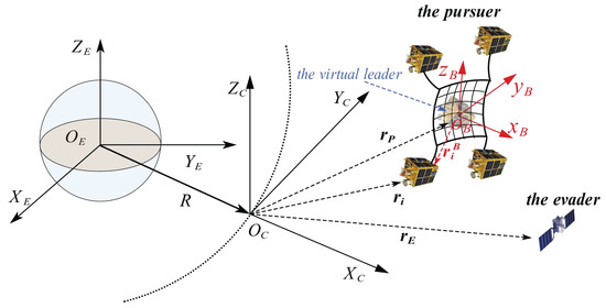
Figure 1.
Graphical representation of the orbital pursuit–evasion system with TSNR.
2.2. Dynamics Modeling
The orbital movement of the spacecraft in the OPEG scenario are represented by defining several coordinate systems based on the earth-centered inertial (ECI) frame, labeled as , which is positioned at the center of the Earth. The relative dynamics between the orbital pursuer and the evader are analyzed in the Euler-Hill coordinate frame. This frame, labeled as , is defined with the -axis pointing radially outward, the -axis aligned with the angular momentum vector, and the -axis completing the right-handed orthogonal coordinate system. To describe the attitude of the tethered net, the body-fixed frame, denoted by , is defined and located at the virtual leader. The -axis aligns with the direction of the virtual leader’s velocity, the -axis is parallel to the plane, and the -axis is defined to form a right-handed orthogonal coordinate system. In the Euler–Hill coordinate frame, the spacecraft’s relative translational dynamics are governed by the following equations:
Here, represents the mean motion of the Euler–Hill coordinate frame, and denotes the acceleration vector generated by continuous low thrust of the spacecraft. The matrix representation of the relative orbital dynamics in the pursuit–evasion scenario is given as follows:
where , and the input of the pursuer and evader spacecraft is assumed to be bounded by positive constants, as follows: and .
2.3. Leader–Follower Framework Design
The game theory-based virtual leader–follower tracking control framework is shown in Figure 2. Based on initial conditions and the game control strategy, both the virtual leader (the pursuer) and the evader can follow their ideal NE trajectories. Then, using the distributed formation tracking control, the followers with a tethered net can track their formation trajectory under the uncertainty of tethered net dynamics and safety constraints.
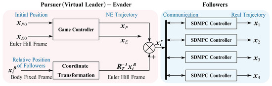
Figure 2.
Diagram illustrating the structure of the proposed leader–follower scheme.
Furthermore, as illustrated in Figure 3, minimizing the impact of the evader on the net during capture requires reducing the angle between the velocity vectors of the virtual leader and the evader ( and ), as well as the angle between the net’s normal vector and the virtual leader’s velocity . Aligning these vectors will help ensure a smoother interception and mitigate potential deformation or damage to the net.
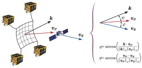
Figure 3.
Diagram illustrating the capture angle.
To minimize the angle , the virtual leader’s strategy is optimized by minimizing the objective function , which reflects the velocity error between the virtual leader and the evader. In addition, to reduce the angle , the desired relative states of the follower spacecraft are defined in the body-fixed frame such that the vector is aligned with the -axis, which is oriented along the virtual leader’s velocity vector, namely denoted by . The state of the ith follower in the body-fixed frame is designed to achieve the desired formation configuration. By applying a coordinate transformation involving the rotation matrix and translation vector (representing the state of the virtual leader), we can obtain the reference state for the ith follower spacecraft in the Euler–Hill frame as follows:
where is defined as follows:
Here, the two rotation angles and of the coordinate axes are defined as follows:
3. Game Theory-Based Approach to Orbital Pursuit–Evasion Problem
3.1. OPEG Modeling
In the OPEG, two players are involved: a virtual leader and an evader. The spacecraft’s cost function is formulated as follows:
where denotes the initial state at time and is a positive definite matrix. Additionally, to handle the input saturation constraints of the spacecraft, this section introduces a non-quadratic function , which is expressed as follows [23]:
where is a positive definite diagonal matrix and denotes the inverse of the hyperbolic tangent function. can be reduced to a form that no longer includes the integral symbol, as shown below:
where the vector , . denotes the natural logarithm (base e), while indicates that each component of the vector is squared individually.
In this OPEG scenario, the virtual leader designs a control to minimize , while the evading spacecraft designs a control to maximize it. This optimal control problem, involving both the virtual leader and evader, is a zero-sum game with a unique solution if a NE strategy exists, provided that the following condition holds.
3.2. Approach to Game Control Solution
The value function is defined as follows:
Based on the Taylor expansion of the value function V, the equivalent expression of Equation (10) is as follows:
The Hamiltonian is defined as follows:
Based on the stationary conditions of optimization, the optimal controls are derived by solving the following first-order conditions:
Accordingly, the game controls of the two players can be expressed as follows:
where denotes the hyperbolic tangent function and is defined as follows:
Substituting Equations (8) and (13) into Equation (11) gives the following the Hamilton–Jacobi–Isaacs (HJI) equation:
By solving the HJI equation, the optimal value function is obtained and subsequently substituted into Equation (13) to derive the NE game controls for the virtual leader and the evader, which are . However, due to the nonlinearities in the cost terms and the presence of input saturation, the HJI equation cannot be solved analytically. Nevertheless, its explicit form is essential for constructing the loss function used in the neural network-based approximation of the value function. To address this, the ADP method is employed to obtain a numerical solution under input constraints. The neural network can be employed to approximate the optimal value function and its gradient , as follows:
where denotes the ideal constant weight vector, is a vector of manually designed basis functions that act as neuron nodes, and represents the approximation error of the neural network. Then, the gradient form of is given as follows:
Let denote the estimation of , and the estimation of the gradient of the value function can be described as follows:
The NE control can be approximated as follows:
Substituting Equations (19) and (20) into Equation (12), we can obtain the estimation error of the HJI equation as follows:
To approximate the solution of the HJI equation, the approximation error is expected to be minimized as much as possible. By minimizing the squared error term , the learning of the neural network weight vector can be achieved. Based on this, the updated law for the weight vector is defined as follows:
where the is the learning rate, . An enhanced Levenberg–Marquardt algorithm modifies the normalization denominator from to , ensuring boundedness in the mathematical proof [23]. By performing iterative updates of the form , the neural network weights are expected to converge, allowing for the determination of the game control for the spacecraft in the OPEG.
4. SDMPC Approach to Multi-Agent Formation Control
4.1. Task Formulation for Formation Control
In this section, we examine a scenario in which four follower spacecraft cooperatively maneuver a tethered net to track the NE trajectory of a virtual leader. Effective coordination among the followers is essential for successful mission execution, necessitating synchronized decision-making. Each follower is required to reach its assigned position while maintaining the prescribed formation configuration. To ensure coordinated operation, the system must comply with the completeness constraints imposed on each follower spacecraft, specified as follows:
where represents the reference position of the ith follower, computed according to Equation (3); denotes the desired relative positions among the followers, while R and r represent the maximum and minimum safe distances between followers, respectively. Let be the index set of the four follower spacecraft. is a priori information for agent i denotes the set of neighbors of agent i.
In this work, SDMPC is employed to facilitate formation tracking while ensuring compliance with critical constraints and mitigating the effects of disturbances caused by the tethered net. These constraints not only involve maintaining safe inter-spacecraft distances above, but also require that the gap between the actual trajectories and the assumed trajectories communicated to other agents remains within acceptable bounds. The assumed trajectories are defined as the combination of the optimal trajectories computed at the previous time step and the terminal control input applied to the final state, as shown in Equation (40). The computational schematic of the SDMPC method is illustrated in Figure 4. At kth time step, each spacecraft optimizes its trajectory at the kth time step based on the reference trajectory , the optimized trajectory from the th time step, and the assumed trajectories of its neighboring spacecraft. The corresponding notations for control and state variables are summarized in Table 1. The first segment of the optimized control for each follower is chosen as the actual input at kth time step, and then the actual next state is determined.
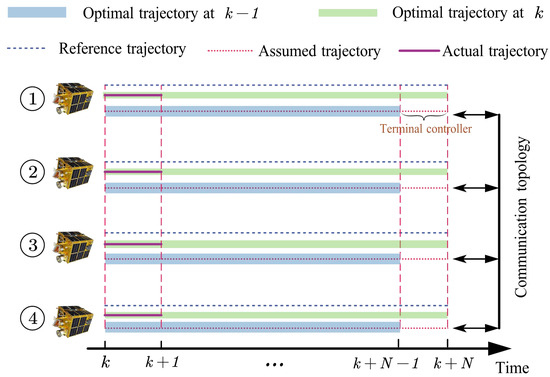
Figure 4.
The computational schematic of the SDMC method for spacecraft formation tracking.

Table 1.
Description of different control and state variables.
4.2. Definition of the Cost Functions and Constraints
At time step k, the cost function for ith follower can be written in the following form.
with the constraint that for ,
where
Equations (28) and (29) represent the dynamic constraints and input saturation constraints, respectively. Equations (30) and (31) impose safety constraints induced by the tethered nets. Similarly, Equation (32) define the compatibility constraints, while Equation (33) specifies the terminal state region constraints. The cost function in this optimal problem is expressed as follows:
where the stage and terminal cost functions are defined as follows:
where denotes the squared weighted norm of a vector with respect to the matrix , i.e., .
4.3. Design of the Compatibility Constraints
To ensure formation tracking consistency in synchronized decision-making, it is assumed that each agent’s actual trajectory has a small deviation from its assumed trajectory communicated to other agents. To address this, the compatibility constraint on position in this work is defined as follows:
4.4. Design of Safety Constraints
Considering the configuration constraints of the tethered net deployment, the tracking spacecraft must satisfy the following safe distance constraints:
4.5. Design of the Terminal Ingredients
4.5.1. Terminal Control
The assumed control and assumed state, which include the optimal solution from the previous step and the terminal component, are defined as follows:
The terminal control in assumed control is constructed as follows:
Substitute the terminal control into the orbital dynamics (Equation (1)) and express them in the following difference form.
The gains and are computed such that the matrix is stabilized, and the equality holds. This expression can be further simplified as follows:
4.5.2. Terminal Cost
The terminal cost is defined in Equation (36), where is a positive definite matrix obtained as the solution to the Lyapunov equation, commonly represented as follows:
where is a predefined matrix with positive definite. Additionally, it can be demonstrated that the terminal cost serves as a local control-Lyapunov function and satisfies the following conditions. The detailed derivation is omitted here, as a similar process can be found in [24]:
4.5.3. Terminal Set
4.6. Discussion of the Feasibility and Stability
At the kth time step, all follower spacecraft independently solve their respective optimization problems simultaneously. Provided a feasible solution exists at the initial time for each follower spacecraft, the optimization problem remains feasible at all subsequent time steps. Moreover, the entire system converges to a state of asymptotic stability.
Proof.
(a) Feasibility: At the kth time step, it is assumed that a valid solution exists for the formation tracking of the follower spacecraft. Let the assumed control and assumed state be the feasible control and feasible state . Since and is derived from the constrained optimization at the kth time step, it readily satisfies the constraints such as Equations (28)–(32). Additionally, under the designed feedback control , the positively invariant set ensures that the safety constraints are met. Therefore, if a feasible solution exists at the kth time step in this optimization problem of each follower spacecraft, a feasible solution will also exist at the th time step.
(b) Stability: The difference in the sum of optimal costs for all spacecraft between consecutive time steps can be expressed as follows:
Further simplification can be obtained by substituting Equation (45) into the above, given that is a quadratic form defined by a positive semi-definite matrix, yielding the following:
□
5. Simulation Results
In this section, numerical simulations are conducted based on the initial conditions to evaluate the proposed game theory-based virtual leader–follower control in addressing the multi-agent OPEG problem. In this study, the initial states of the virtual leader and the evader, along with the desired relative state of the follower are provided in Table 2. For each simulation, the position of the evader is randomly selected within a certain range. The local orbital angular velocity is set to . The coefficient affecting the maximum input of the virtual leader is specified as , while the evader’s is limited to [25]. Select , [23]. Additionally, the capture threshold m. The learning rate [26], and the activation function employed to approximate the optimal value function is chosen as follows:
which results in a single hidden layer neural network architecture with 27 neuron nodes for approximating the optimal value function. The initial values of the neural network weights for the iterative process are given as follows:
Table 2.
Initial states of the spacecraft in Euler–Hill frame, and expected relative state between followers in body-fixed frame.
To enrich the states for training neural network weights, we injected random noise into the x-axis control input of the virtual leader during the first 80 s.
Additionally, the prediction horizon length N is set to 6, and the time step s. Considering the safety issues of each follower during formation tracking, the minimum distance between adjacent pursuers is set as m, and the maximum distance between them is denoted as m. The adjacency matrix that defines the communication topology among the followers is defined as follows:
In this work, based on the initial condition , the simulation results of the OPEG are presented in Figure 5, Figure 6, Figure 7, Figure 8, Figure 9, Figure 10, Figure 11, Figure 12, Figure 13 and Figure 14. Specifically, Figure 5 illustrates the NE trajectories of both spacecraft, while Figure 6 depicts the evolution of the distance between them. From these figures, it can be observed that the evader attempts to escape, whereas the virtual leader actively minimizes the distance . Due to its higher acceleration capability, the virtual leader gradually closes their gap over time and captures the evader. Figure 7 illustrates the convergence behavior of the neural network weights, which eventually stabilize at specific values as follows:
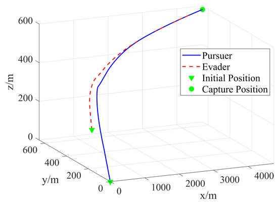
Figure 5.
Trajectories of the virtual leader and the evader during the OPEG.
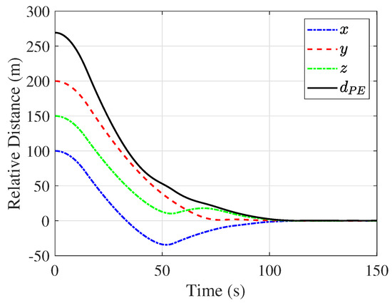
Figure 6.
Relative position between the virtual leader and the evader during the OPEG.
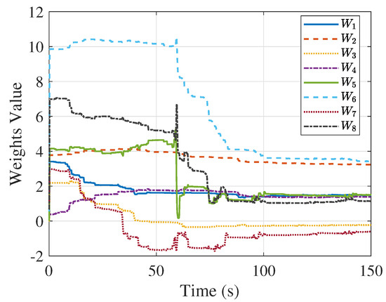
Figure 7.
Convergence of the weights of the optimal value function.
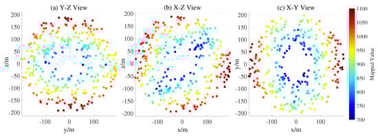
Figure 8.
Colored scatter plot of initial positions, annotated by control effort.
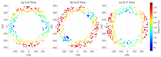
Figure 9.
Colored scatter plot of unseen initial positions, annotated by capture time.
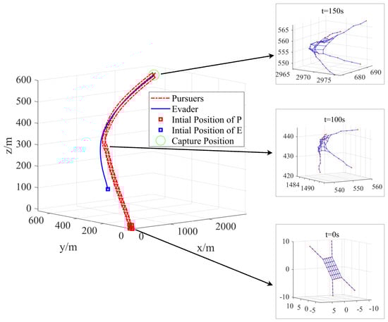
Figure 10.
Trajectories of the followers and configuration of the tethered net under the formation tracking control.
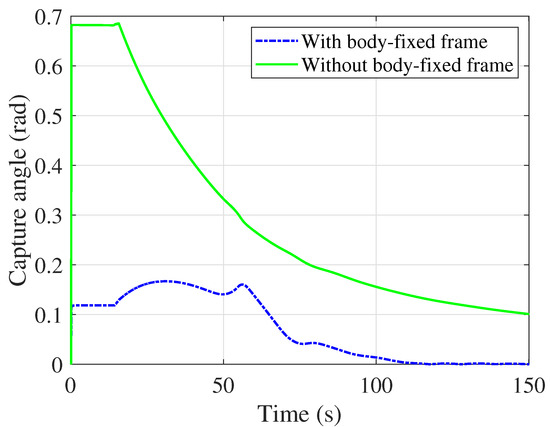
Figure 11.
The variation in the capture angle under two different reference trajectories during formation tracking.
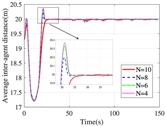
Figure 12.
The average inter-agent distance with different predictive horizons.
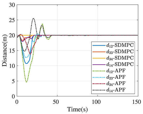
Figure 13.
Comparison of formation distance variations with the APF method.
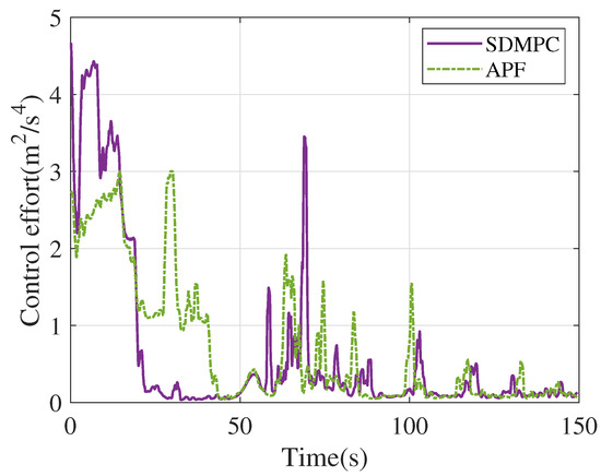
Figure 14.
Comparison of input variations with the APF method.
The weight convergence condition is defined based on the infinity norm of the difference between two consecutive weight vectors. Specifically, the training is considered to have converged when . The NE control can be obtained for both virtual leader and evader by substituting the converged weights into Equation (18). Based on this control strategy, we conducted 600 randomized simulations to investigate how the relative initial positions between the evader and the virtual leader influence the capture outcome. The evader’s initial positions are sampled in the YZ, XZ, and XY planes that pass through the origin. Under this NE control policy, all simulations resulted in successful capture within 100 s. Moreover, the control effort required by the virtual leader is generally positively correlated with the initial distance to the evader, as illustrated in Figure 8. To further evaluate the generalization ability of the NE control policy, we expand the sampling region of the evader’s initial positions to an unseen area and conduct another 600 randomized simulations. The results are shown in Figure 9, where red crosses denote evader initial positions that were not captured within 300 s, and the color of each point indicates the required capture time. A success rate of 95.16% is achieved in the unseen region, demonstrating the generalization capability of the proposed NE control policy.
Based on the NE trajectory of the virtual leader, Figure 10 illustrates the trajectory and configuration of the TSNR system based on SDMPC control during the formation tracking simulation. Three representative states of the tethered net’s motion are highlighted in the figure. The blue segments of the tethered net indicate the distances between neighboring nodes. When the relative distances among the four follower spacecraft remain within an appropriate range, the net maintains slight tension, contributing to overall system stability. Furthermore, by defining the reference trajectories of the followers in the body-fixed frame rather than the Euler–Hill frame, the capture angle during the net-capturing process can be effectively reduced, and its supporting simulation result is shown in Figure 11. In addition, a simulation analysis was conducted to evaluate the formation control performance under different predictive horizons, as illustrated in Figure 12. The vertical axis represents the average distance between adjacent spacecraft. The results show that a larger predictive horizon slightly improves formation control performance, but it also leads to increased computational load. Specifically, as the prediction horizon increases from to , the average computation time per prediction step increases from 0.18 s to 0.25 s, 0.33 s, and 0.46 s, respectively.
To further demonstrate the advantages of the proposed SDMPC approach, a comparative analysis is conducted against the APF method, a widely acknowledged state-of-the-art technique in formation tracking applications [7]. As shown in Figure 13, the real-time lengths of the formation edges are illustrated, demonstrating that the proposed SDMPC approach achieves the desired formation more quickly and effectively mitigates overshoot caused by the dynamics of the tethered net. Additionally, Figure 14 presents the control effort of the follower spacecraft under both methods; the total control effort consumed by SDMPC is 938.26 , compared to 1060.04 by APF.
To ensure the generalizability of the results, 600 Monte Carlo simulation runs were conducted with randomized initial positions of the evader during the pursuit–evasion phase. Figure 15 presents the trajectory and formation configuration of the TSNR system under SDMPC-based tracking, corresponding to the initial condition . This Monte Carlo simulation also provided sufficient data to support a statistical comparison of performance metrics across different formation tracking methods. The performance metrics include control effort, maximum formation deviation, and formation error convergence time. Specifically, control effort represents the energy cost of control; maximum formation deviation denotes the largest error in the distance between adjacent spacecraft compared to the desired spacing; and formation error convergence time refers to the time required for the maximum formation deviation to fall below 0.5 m. As shown in Table 3, the proposed SDMPC method controls formation errors more effectively while also achieving lower control effort consumption.
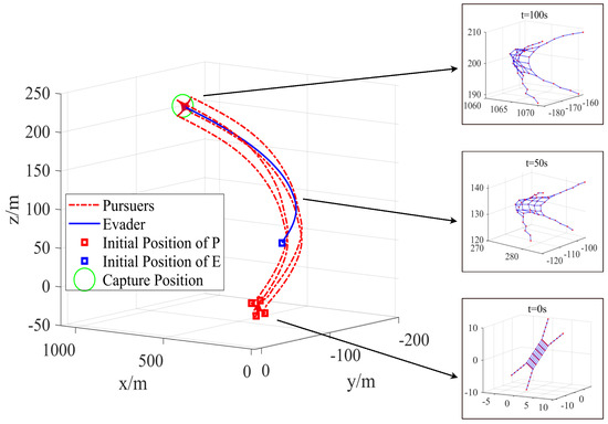
Figure 15.
Trajectories of the followers and configuration of the tethered net under the formation tracking control with .
Table 3.
Comparison of performance metrics (mean ± standard deviation) between SDMPC and APF.
6. Conclusions
In this study, a game-theoretic virtual leader–follower tracking control strategy is proposed for orbital pursuit–evasion systems involving tethered space net robots. At the OPEG level involving the virtual leader and the evader, an ADP approach incorporating a saturation function is employed to effectively handle input constraints and compute the NE trajectories for this orbital zero-sum game. At the formation tracking level, the follower’s SDMPC strategy ensures robust formation tracking performance under safety constraints and uncertain net dynamics, with theoretical analysis provided for feasibility and stability. The Monte Carlo simulation results demonstrate that the proposed system can successfully capture the target while maintaining safe inter-spacecraft distances, outperforming existing formation tracking methods in both formation maintenance and control effort. Additionally, the designed capture strategy maintains a small capture angle, which helps reduce the impact force on the tethered net during engagement. Additionally, it is worth noting that the communication conditions considered in this work are relatively idealized. In future work, we plan to further account for communication delays, noise, and packet loss to enhance the robustness of the system’s cooperative control.
Author Contributions
Conceptualization, Z.Z. and C.W.; methodology, C.W.; software, C.W.; validation, C.W. and J.L.; formal analysis, Z.Z. and C.W.; investigation, C.W.; data curation, C.W.; writing—original draft preparation, C.W.; writing—review and editing, Z.Z. and C.W.; visualization, C.W.; funding acquisition, J.L. All authors have read and agreed to the published version of the manuscript.
Funding
This research is supported by the National Natural Science Foundation of China under Grant No. 12072269, and the Innovation Foundation for Doctor Dissertation of Northwestern Polytechnical University under Grant No. CX2021049.
Data Availability Statement
The data presented in this paper are available on request from the corresponding author.
Conflicts of Interest
The authors declare no conflicts of interest.
References
- Aglietti, G.S.; Taylor, B.; Fellowes, S.; Salmon, T.; Retat, I.; Hall, A.; Steyn, W.H. The active space debris removal mission RemoveDebris. Part 2: In orbit operations. Acta Astronaut. 2020, 168, 310–322. [Google Scholar] [CrossRef]
- Svotina, V.V.; Cherkasova, M.V. Space debris removal–Review of technologies and techniques. Flexible or virtual connection between space debris and service spacecraft. Acta Astronaut. 2023, 204, 840–853. [Google Scholar] [CrossRef]
- Liu, Y.; Ma, Z.; Zhang, F.; Huang, P. Time-varying formation planning and scaling control for tethered space net robot. IEEE Trans. Aerosp. Electron. Syst. 2023, 59, 6717–6728. [Google Scholar] [CrossRef]
- Zhu, W.; Pang, Z.; Du, Z.; Gao, G.; Zhu, Z.H. Multi-debris capture by tethered space net robot via redeployment and assembly. J. Guid. Control Dyn. 2024, 10, 1359–1376. [Google Scholar] [CrossRef]
- Zhang, F.; Huang, P. Releasing dynamics and stability control of maneuverable tethered space net. IEEE/ASME Trans. Mechatron. 2016, 22, 983–993. [Google Scholar] [CrossRef]
- Ma, Y.; Zhang, Y.; Liu, Y.; Huang, P.; Zhang, F. An active energy management distributed formation control for tethered space net robot via cooperative game theory. Acta Astronaut. 2025, 227, 57–66. [Google Scholar] [CrossRef]
- Ma, Y.; Zhang, Y.; Huang, P.; Liu, Y.; Zhang, F. Game theory based finite-time formation control using artificial potentials for tethered space net robot. Chin. J. Aeronaut. 2024, 37, 358–372. [Google Scholar] [CrossRef]
- Du, Z.; Zhang, H.; Wang, Z.; Yan, H. Model predictive formation tracking-containment control for multi-UAVs with obstacle avoidance. IEEE Trans. Syst. Man Cybern. Syst. 2024, 54, 3404–3414. [Google Scholar] [CrossRef]
- Nie, Y.; Li, X. Antidisturbance distributed lyapunov-based model predictive control for quadruped robot formation tracking. IEEE Trans. Ind. Electron. 2025. [Google Scholar] [CrossRef]
- Li, J.; Li, C. Guidance strategy of motion camouflage for spacecraft pursuit-evasion game. Chin. J. Aeronaut. 2024, 37, 312–319. [Google Scholar] [CrossRef]
- Jia, Z.; Ye, D.; Xiao, Y.; Sun, Z. Closed-Loop Strategy Synthesis for Real-Time Spacecraft Pursuit-Evasion Games in Elliptical Orbits. IEEE Trans. Aerosp. Electron. Syst. 2025. [Google Scholar] [CrossRef]
- Liu, Y.; Zhang, Y.; Jiang, J.; Li, C. Multiple-to-one orbital pursuit: A computational game strategy. IEEE Trans. Aerosp. Electron. Syst. 2024, 61, 2213–2225. [Google Scholar] [CrossRef]
- Shen, H.; Casalino, L. Revisit of the three-dimensional orbital pursuit-evasion game. J. Guid. Control Dyn. 2018, 41, 1820–1831. [Google Scholar] [CrossRef]
- Shen, M.; Wang, X.; Zhu, S.; Wu, Z.; Huang, T. Data-driven event-triggered adaptive dynamic programming control for nonlinear systems with input saturation. IEEE Trans. Cybern. 2023, 54, 1178–1188. [Google Scholar] [CrossRef]
- Lv, Y.; Ren, X. Approximate Nash solutions for multiplayer mixed-zero-sum game with reinforcement learning. IEEE Trans. Syst. Man Cybern. Syst. 2018, 49, 2739–2750. [Google Scholar] [CrossRef]
- Zhang, T.; Zhang, S.; Li, H.; Zhao, X. Velocity-free prescribed-time orbit containment control for satellite clusters under actuator saturation. Adv. Space Res. 2025, 75, 5110–5123. [Google Scholar] [CrossRef]
- Yao, Q.; Li, Q.; Xie, S.; Jahanshahi, H. Distributed predefined-time robust adaptive control design for attitude consensus of multiple spacecraft. Adv. Space Res. 2025, 75, 7473–7486. [Google Scholar] [CrossRef]
- Wei, C.; Wu, X.; Xiao, B.; Wu, J.; Zhang, C. Adaptive leader-following performance guaranteed formation control for multiple spacecraft with collision avoidance and connectivity assurance. Aerosp. Sci. Technol. 2022, 120, 107266. [Google Scholar] [CrossRef]
- Xue, X.; Wang, X.; Han, N. Leader-Following Connectivity Preservation and Collision Avoidance Control for Multiple Spacecraft with Bounded Actuation. Aerospace 2024, 11, 612. [Google Scholar] [CrossRef]
- Grimm, F.; Kolahian, P.; Zhang, Z.; Baghdadi, M. A sphere decoding algorithm for multistep sequential model-predictive control. IEEE Trans. Ind. Appl. 2021, 57, 2931–2940. [Google Scholar] [CrossRef]
- Wu, J.; Dai, L.; Xia, Y. Iterative distributed model predictive control for heterogeneous systems with non-convex coupled constraints. Automatica 2024, 166, 111700. [Google Scholar] [CrossRef]
- Dai, L.; Cao, Q.; Xia, Y.; Gao, Y. Distributed MPC for formation of multi-agent systems with collision avoidance and obstacle avoidance. J. Franklin Inst. 2017, 354, 2068–2085. [Google Scholar] [CrossRef]
- Mu, C.; Wang, K. Approximate-optimal control algorithm for constrained zero-sum differential games through event-triggering mechanism. Nonlinear Dyn. 2019, 95, 2639–2657. [Google Scholar] [CrossRef]
- Jiang, Y.; Hu, S.; Damaren, C.; Luo, L.; Liu, B. Trajectory planning with collision avoidance for multiple quadrotor UAVs using DMPC. Int. J. Aeronaut. Space Sci. 2023, 24, 1403–1417. [Google Scholar] [CrossRef]
- Zhu, W.; Pang, Z.; Si, J.; Gao, G. Dynamics and configuration control of the Tethered Space Net Robot under a collision with high-speed debris. Adv. Space Res. 2022, 70, 1351–1361. [Google Scholar] [CrossRef]
- Yang, Y.; Fan, X.; Xu, C.; Wu, J.; Sun, B. State consensus cooperative control for a class of nonlinear multi-agent systems with output constraints via ADP approach. Neurocomputing 2021, 458, 284–296. [Google Scholar] [CrossRef]
Disclaimer/Publisher’s Note: The statements, opinions and data contained in all publications are solely those of the individual author(s) and contributor(s) and not of MDPI and/or the editor(s). MDPI and/or the editor(s) disclaim responsibility for any injury to people or property resulting from any ideas, methods, instructions or products referred to in the content. |
© 2025 by the authors. Licensee MDPI, Basel, Switzerland. This article is an open access article distributed under the terms and conditions of the Creative Commons Attribution (CC BY) license (https://creativecommons.org/licenses/by/4.0/).