Abstract
In recent years, with the development of micro-satellite clusters and large-scale satellite constellations, the likelihood of multiple spacecraft engaging in orbital pursuit–evasion games has increased. This paper establishes a novel interception domain theory for planar orbital multi-player “encirclement-capture” differential games, and it proves the partitioned structure and classification properties of Nash equilibrium solutions. The main contributions of our study are the following: (1) Proposing the first rigorous definition of interception domains in orbital pursuit–evasion games, proving their convexity, developing computational methods for domain intersections, and establishing a complete classification of equilibrium for planar multi-pursuer interception games, which establishes a theoretical foundation for analyzing multi-spacecraft orbital pursuit–evasion games. (2) Analyzing Nash equilibrium properties for “encirclement-capture” differential games with two, three, or more pursuers, classifying degenerate/non-degenerate scenarios via spatial inclusion relationships. The equilibrium results indicate that as the number of pursuers increases, the game tends toward a degenerate scenario where the likelihood of redundant pursuers (whose actions do not affect the game outcome) rises.
1. Introduction
Spacecraft orbital games describe strategic interactions between adversarial spacecraft groups governed by orbital dynamics and operational constraints. The theoretical foundation for the differential game approach was established in the 1970s when Anderson and Grazier [1] pioneered the application of Isaacs’ differential game framework [2] to low Earth orbit scenarios, formulating the first orbital pursuit–evasion differential game model for spacecraft employing continuous low-thrust propulsion systems. With the growing significance of the space domain, orbital differential pursuit–evasion game modeling has emerged as a critical research focus [3]. Current studies encompass scenarios where both parties optimize their control strategies based on objectives such as relative distance, fuel consumption, and game duration.
In recent years, the advancement of micro-satellite clusters and large-scale satellite constellations (e.g., EAGLE) has significantly increased the occurrence of multi-spacecraft orbital games [4]. In such settings, engagements with only one or two pursuers constitute special cases. This trend has drawn growing attention to orbital pursuit–evasion problems involving multiple participants. A particularly important variant is the multi-player “encirclement-capture” game, in which multiple cooperative pursuers strategically coordinate to capture a single evader.
Studying such multi-pursuer scenarios is essential. Cooperative pursuers can leverage tactical advantages—such as coordinated maneuvering and spatial occlusion—to achieve interception more quickly and reliably than in single-pursuer engagements. Moreover, as the number of pursuers increases, new strategic dilemmas and equilibrium types emerge—reflecting qualitative, not merely quantitative, changes in game outcomes. The strategies and outcomes vary considerably depending on the number and configuration of pursuers. Therefore, a systematic classification of game scenarios is crucial both for theoretical understanding and practical application. These capabilities play a critical role in applications such as constellation configuration design and space situational awareness.
Within that context, this paper seeks to address the following research questions:
- What are the optimal pursuit strategies for the pursuer group and the optimal evasion strategies for the evader?
- Can all pursuers either intercept the evader or meaningfully influence the game outcome?
- How does the number of pursuers affect interception performance and game dynamics?
Existing research on orbital pursuit–evasion games has primarily focused on one-to-one scenarios. For instance, Pontani and Conway [5] investigated interception scenarios between two remote spacecraft employing constant-thrust propulsion. Building upon this work, Shen and Casalino [3] extended the framework by incorporating constraints such as minimum orbital altitude requirements and time-varying spacecraft mass dynamics. Stupik et al. [6] examined games involving spacecraft satisfying the Clohessy–Wiltshire (CW) conditions, which were further studied by Zhang et al. [7] using deep neural network methodologies. The pursuit–evasion games under imperfect information have been analyzed using various approaches, including compensation control strategies [8], different sensor schemes [9], a two-stage game model [10], mode-matched smooth variable structure filters [11], and a parameter-optimized control method based on the receding horizon framework [12]. Li et al. [13] further expanded the model to account for J2 gravitational perturbations. The pursuit–evasion games with fuel consumption as the optimization objective have been covered by the studies of discrete thrust conditions [14], optimization of total velocity increments [15], and reachable domains with fixed velocity increments [16]. The pursuit–evasion games with sun angle constraints have been covered by the studies of inspection games [17] and observation and counter-observation games [18]. Separately, Jagat and Sinclair conducted studies on orbital rendezvous scenarios, analyzing both linear [19] and nonlinear [20] dynamic systems, with optimization objectives centered on minimizing relative distance and fuel expenditure during maneuvering phases. Furthermore, research on multi-spacecraft orbital games has largely concentrated on pursuit–evasion–defense tripartite games, where an evader deploys a defender to intercept the pursuer. This problem has roots in studies on missile–target–interceptor tripartite games [21]. Within this context, Li et al. [22] analyzed the control strategies and winning conditions of the pursuer and defender by solving the Nash equilibrium under the assumption that the evader cannot maneuver. Li [23] compared scenarios where the evader and defender adopted cooperative versus non-cooperative strategies. They found that cooperative strategies significantly reduce the risk of the evader being captured.
To the best of our knowledge, there are three existing studies on orbital multi-player “encirclement-capture” games, which were conducted by Sun et al. [24], Jansson and Harris [25], and Li et al. [4].
Sun et al. [24] employed differential game theory to investigate the specific case involving exactly two pursuers. They considered non-degenerate scenarios where both pursuers simultaneously intercept the evader and degenerate scenarios where one pursuer cannot influence the game outcome, providing corresponding degeneracy determination algorithms. However, they did not provide a systematic theoretical proof for this classification—for example, why there cannot be a non-degenerate scenario where only one pursuer achieves interception. As demonstrated by the results in this paper, there are essential differences between two-pursuer and three-or-more-pursuer games, which indicates that their approach has limitations, whereas the interception-domain-based methodology proposed in this paper offers greater universality for this problem. The part of our research on two-versus-one games essentially provides a theoretical verification and supplementary proof for their study, while also offering a scenario discrimination algorithm with lower computational dimensionality.
Jansson and Harris [25] proposed a geometric algorithm based on reachable sets for a general number of pursuers. Their algorithm first computes the time-evolving reachable sets for each spacecraft and then iterates over time to identify the moment and location where the evader’s reachable set first becomes fully covered by the pursuers’ collective reachable sets. While their reachable set approaches may compute different degenerate or non-degenerate cases, they cannot answer which scenarios are possible and which are impossible—a key research question addressed in this paper. Furthermore, our method is distributed and hierarchical: it first efficiently identifies active pursuers via low-dimensional calculations before solving for trajectories, making it particularly suitable for rapid decision-making in large-scale encounters.
Li et al. [4] derived cooperative capture strategies for multiple spacecraft using discrete impulses as the maneuvering method, along with corresponding evasion strategies, via an effective deep reinforcement learning algorithm designed for multi-player cooperative games. Unlike their work, which relies on discrete impulses and learning algorithms, this paper presents theoretical Nash equilibrium solutions under the assumption of continuous low-thrust maneuvers. Thus, our results are more applicable to low-thrust propulsion systems such as electric propulsion satellites. In addition, compared to results derived from deep reinforcement learning, the differential game-based solutions obtained in this study possess theoretical optimality guarantees and offer higher interpretability.
Additionally, some studies have explored general multi-player “encirclement-capture” games without orbital dynamics constraints. For instance, Jin and Qu [26] investigated the barriers of the game under scenarios where players can control both the magnitude and direction of their velocity in real time, while Chen et al. [27] studied the barriers when players can control their velocity magnitude and angular velocity magnitude of direction in real time. In contrast, to align with practical spacecraft maneuvering, the scenario considered in this paper is more complex. First, in our model, spacecraft can only control their thrust direction, not their velocity directly. Second, all spacecraft in our model remain subject to gravitational fields. As will be shown later, these differences significantly increase the complexity of solving the proposed model.
To fill the theoretical gap in orbital “encirclement-capture” games, particularly concerning the classification of scenarios involving more than two pursuers, this paper establishes a differential game model for such games. We establish a novel interception domain theory to establish a complete classification of equilibrium for planar multi-pursuer interception games. The main contributions of our study are summarized as follows: (1) We propose and define the interception domain, which establishes a theoretical foundation for analyzing multi-spacecraft orbital pursuit–evasion games. (2) We model “encirclement-capture” differential games involving two, three, or more pursuers, determine their Nash equilibrium solutions, and prove the partitioned structure and classification properties of the solutions.
The remainder of this paper is organized as follows: Section 2 introduces the setup of the differential model for the “encirclement-capture” game and defines the problem to be solved. Section 3 defines and discusses the interception domain. Section 4 describes the derivation of the two-pursuer Nash equilibrium solution. Section 5 describes the derivation of the three-pursuer Nash equilibrium solution. Section 6 describes the derivation of the Nash equilibrium solution when there are more than three pursuers. Section 7 shows simulation examples. Section 8 concludes the paper.
2. Differential Game Model
Consider a game scenario involving multiple pursuers collaborating to intercept an evader. Upon initiation of the game, all players acquire real-time state information of other players, including positional coordinates, velocity vectors, and maneuvering acceleration magnitudes. Each player executes corresponding continuous control strategies optimized for their respective objectives. The game terminates when at least one pursuer achieves physical coincidence with the evader. During the game process, the pursuers aim to minimize mission completion time, while the evader seeks to maximize it.
The dynamics in this work are restricted to planar motion governed by CW dynamics, a simplification justified by the specific orbital environment under consideration—namely, geostationary orbit (GEO), which is the main scenario of orbital games, especially multi-spacecraft orbital games [28]. Satellites in GEO are required to perform strict north–south station-keeping maneuvers to maintain their orbital inclination within a very small range (typically within ±0.05° to ±0.1° [29]). This practice effectively suppresses out-of-plane motion, making the planar assumption a valid and widely adopted approximation for analyzing proximate orbital maneuvers in this regime [1,25]. This model allows us to derive fundamental insights into the multi-pursuer interception problem, which serves as a critical foundation for future extensions.
Denote as the number of the pursuers. Let the positional and velocity vectors (as shown in Figure 1) be defined in a rotating reference frame centered at a circular orbital base.
where the subscripts indicate the variables for each pursuer, respectively, and the subscript indicate the variables for the evader. These vectors serve as the differential game’s state variables.
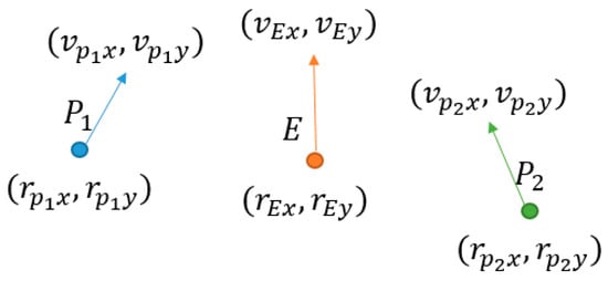
Figure 1.
State variables of the game.
The maneuvering accelerations of players are denoted by thrust magnitude with directions for , where is continuous over the interval and is assumed to be constant for each player. This fixed-thrust-magnitude assumption is standard in time-optimal orbital pursuit–evasion games [3,5]. It is justified by the fact that for a linear system of differential equations, each player will always maintain their maximum thrust in the game equilibrium [2].
Building on prior research [8], let denote the angular velocity of the relative circular orbit. The dynamic equations for each spacecraft are expressed as follows:
Since , there are equations in (2). Denote the right side of them as . The decision variables for this game are the thrust acceleration direction angles of all players, which are assumed to be a function that varies over time . Under a fixed initial state, the game duration becomes a function depending solely on the decision variables. To meet the Nash equilibrium conditions of the game, these decision variables satisfy the following conditions:
Within the framework of optimal control theory, the resolution of constrained optimization problems involving state trajectories adhering to dynamic equations necessitates the introduction of dimensionally equivalent costate variables. For this system, these costate variables are formally defined as . Then, according to Isaac’s differential game theory [2], the second form of the main equation is
where is the time accumulation objective function of the game. In this paper, since the objective function is the duration time. Guided by the Path Equation Theorem, after differentiating (4) with respect to each state variable, the dynamic equations of the costate variables under the Nash equilibrium can be obtained:
Note that (5) is a linear system of differential equations, indicating that the time-varying functions of the costate variables can be directly determined by the boundary values at one end. Next, according to main equation theorem [2], the decision variables satisfy the following conditions:
The above formulas are equivalent to
The optimal direction angle from (7) is computed in real time and provides an inertial pointing command. The spacecraft’s attitude control system must align the thruster with this direction, followed by firing at maximum thrust. This reflects the standard guidance–actuation separation in spacecraft implementation.
By substituting (7) into (2), we obtain a linear system of differential equations governing the state variables. The resulting equations for the pursuers are as follows:
where . The resulting equation for the evader is as follows:
In general differential games, coupling (2) and (5) transforms the problem into a two-point boundary value problem (TPBVP). In this TPBVP, the initial states are known, and the terminal conditions are defined by the game’s termination region. However, in our problem, the termination region involves complex conditional criteria that prevent the direct application of the standard TPBVP approach. Due to this increased complexity, we instead conduct a geometric analysis of the equilibrium properties.
3. Interception Domain
Consider a scenario where a pursuer () attempts to intercept an evader () in minimum time, assuming possesses superior maneuvering capability compared to . In this case, if the evader aims to maximize the interception time, the equilibrium for this game has been analyzed in prior studies [3,5]. Due to the uniqueness of the Nash equilibrium in this differential game, the evader’s trajectory from the start of the game until interception is deterministic. If deviates from this equilibrium strategy for any purpose, it will be intercepted by in less time and via a different trajectory. Evidently, the region reachable by before interception is finite. We define this region as the interception domain. The distinction between the concepts of the interception domain and the reachable set [25] is summarized in Table 1.

Table 1.
Distinction between the concepts of the interception domain and the reachable set.
It is important to note that, distinct from the concept of the reachable set [25], the interception domain is defined by the pair of pursuer and evader, not by a single spacecraft.
We now present the equivalent mathematical definition of the interception domain. For any , consider the following differential pursuit–evasion game: aims to maximize the dot product between the position vector and a given unit vector before interception. Conversely, aims to minimize this value. This game can also be interpreted as a reach–avoid game [30] where the target line is the orthogonal line to the vector . The state and costate dynamics of this game correspond to the single-pursuer case given by (2) and (5) in this paper. The terminal region is the six-dimensional manifold where the position vectors of and coincide. Note that in this game, the objective function is not cumulative over time. By combining the differentiation of with respect to each element of the terminal region and the second form of the main equation, the terminal boundary conditions of TPBVP can be derived as follows:
The solution of the above TPBVP can be assumed as
where the superscript means the corresponding state or costate value in termination.
Due to the smoothness of the solution, the point set forms a closed, smooth curve in the plane. Consider the region bounded by this curve. From the game formulation, it readily follows that at any point on , the tangent line to the curve is the straight line passing through that point and orthogonal to the vector . Furthermore, all points within the region lie on the same side of this tangent line. This implies that the region is convex.
Theorem 1.
The region is the interception domain defined by and .
Proof.
Note that the curve lies within the interception domain .
We first prove that points outside do not belong to the interception domain. Suppose there exists a point outside that the evader can reach under interception by . By the convexity of , there must exist a boundary point such that lies on the opposite side of the tangent line to at this point. According to the definition of , represents the maximum achievable dot product with the vector for under interception. However, the dot product of with is strictly greater, leading to a contradiction.
Points inside clearly belong to the interception domain, though unlike boundary points, trajectories ending at interior points are not unique. For example, can wait for a period of time before maneuvering. □
We have now completed the definition of the interception domain and proven its convexity. As a concrete example, Figure 2 shows a numerical simulation result of an interception domain.
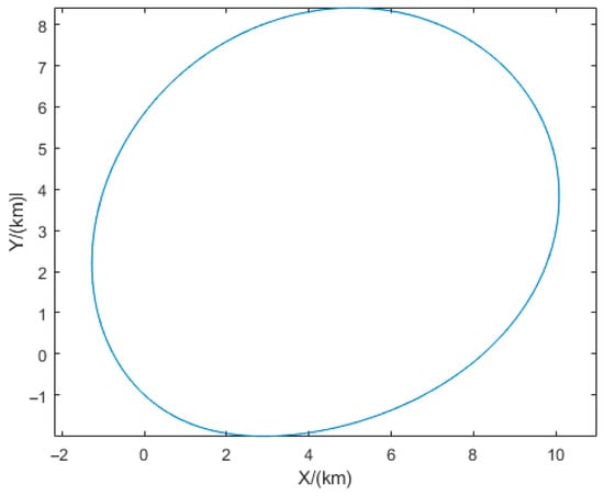
Figure 2.
Numerical simulation result of an interception domain.
In addition, Appendix B explains that under the assumptions of negligible gravitational influence and zero initial velocity for both and , the interception domain will be an Apollonius circle containing scaled according to the ratio of the players’ accelerations (as shown in Figure 3).
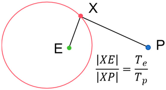
Figure 3.
Interception domain as an Apollonius circle.
In practice, the study by Jansson and Harris [25] found that the relative initial velocity of satellites in geosynchronous orbits and the rotational angular velocity of the coordinate system have a negligible impact on the shape of the reachable set. The reachable set can be closely approximated as a circle centered at the spacecraft. Similarly, our calculations reveal that the interception domain of satellites in geosynchronous orbits is closely approximated by an Apollonius circle, as in Figure 3. Consequently, in subsequent analyses, we assume that the interception domains—or the interception domains relative to the reachable sets—intersect at no more than two points.
Afterwards, our focus will be on the boundary of , which has the following properties.
Proposition 1.
For any point on the curve , the trajectories (i.e., the functions of state variables) for and to simultaneously reach this point determined by (8) are the minimum-time trajectories for and to reach individually.
Proof.
Consider the minimum-time trajectory problem for to reach the point . Following the same methodology as in Section 2, we can formulate the state and costate dynamics equations. It can be readily shown that the boundary conditions for its TPBVP in termination are as follows:
The unique solution to the above TPBVP can be expressed as , representing the minimum time, the evader’s velocity components, and its first two costate components in termination, respectively. Now, consider , where . All elements in are derived from defined by (11).
We now prove that , which is equivalent to verifying that also satisfies (12). From the last two equality conditions in (10), it follows directly that the last two conditions of (12) are satisfied. The first condition of (10) implies that satisfies the first condition in (12). Therefore, we need only prove that the proportional scaling of the first two costate components at termination does not affect the state dynamics governed by (2).
Consider the costate dynamics for governed by (5). When the game duration is and the terminal costate values are , the time evolution of the costate vector is given by
(13) demonstrates that proportional scaling of the first two terminal costates results in proportional scaling of the costate vector at every time instant. By (7), such proportional scaling of the costates does not alter the state dynamics governed by (2). Therefore, .
The equivalence for the pursuer’s minimum-time trajectory to follows analogously by considering the time-optimal control problem of . □
Proposition 1 establishes an exact mathematical property of the interception domain. The uniqueness of the domain itself is inherent to its definition by the initial conditions. While numerical computation of the domain boundary (by solving the associated TPBVP) is subject to the usual sensitivities of boundary value problems, the theoretical scaling law holds exactly for the true domain. In our simulations, the multiple shooting method [22] as a robust numerical method was employed to ensure accurate solutions.
Based on this property, we derive the following corollary, which forms the foundation for applying the concept of the interception domain to the “encirclement-capture” game.
Corollary 1.
If the boundary of the interception domain defined by and
intersects the boundary
defined by
and
at point
, then the minimum times for
,
, and
to reach
are identical. The trajectory for
to reach
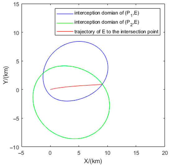
is identical in both interception domains and constitutes its minimum-time trajectory (as shown in Figure 4).
Figure 4.
Trajectory of to the intersection point.
The intersection points of interception domain boundaries, as established in Corollary 1, play a foundational role in defining simultaneous interception events in multi-pursuer games. The property that all players share an identical minimum arrival time at such a point provides the crucial spatiotemporal agreement necessary to coordinate multiple pursuers against a single evader.
For any given pair of pursuers and an evader, the resulting pair of intersection points is unique under specific initial conditions, as it is geometrically determined by their uniquely defined interception domains.
Additionally, an alternative equivalent definition of the interception domain can be given based on Corollary 1: the interception domain is the set of points satisfying the notion that the minimum time for to reach the point is less than or equal to that for . On the boundary of the interception domain, the minimum times for and are exactly equal; in the interior of the interception domain, can arrive before .
4. Orbital Two-Versus-One Pursuit–Evasion Game
Consider a game with two pursuers () and one evader (). Without loss of generality, we set as the reference satellite in the relative coordinate system. Define as the interception domains determined by and , with boundaries , respectively. Under the Nash equilibrium for the one-versus-one pursuit–evasion game between and , both players reach point at time . Similarly, for and , they reach point at time under their Nash equilibrium. For the sake of conciseness, this paper does not address cases where conditional judgments yield equality, as such scenarios occur with Lebesgue measure zero in practice and can be arbitrarily approximated by strict inequality conditions. Thus, without loss of generality, assume .
Consider the relationship between the two interception domains. By definition, both interception domains contain the origin since it is the initial position of , implying a non-empty overlap region . Consequently, the region reachable by prior to interception is precisely . Define as the minimum-time function for player to reach point . Under game equilibrium, the position where is intercepted (hereafter termed the interception point) must satisfy
In addition, by definition, the minimum time for to reach any point within is strictly less than . Consequently, must lie outside . At this stage, the sole determinant of the game equilibrium is whether lies within (as illustrated in Figure 5, and are shown by blue and green regions respectively. Definitions of all points in sketches of the interception domain are summarized in Appendix B). Theorem 2 characterizes the Nash equilibrium solutions under these two distinct scenarios.
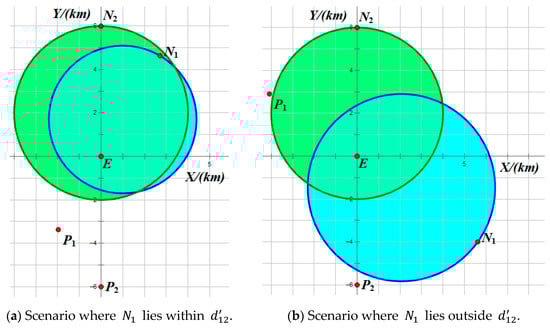
Figure 5.
Sketch of interception domains in two-versus-one pursuit–evasion game.
Theorem 2.
The Nash equilibrium solutions varying based on whether lies within are as follows:
- (1)
- If lies within , the game degenerates into a one-versus-one pursuit–evasion game between and . Under equilibrium, intercepts at point ;
- (2)
- If lies outside , under equilibrium, and simultaneously intercept
Proof.
The proof of (1) is straightforward. Since can reach at time before interception, and is the maximum interception time for within , it is also the maximum interception time within .
The proof of (2) proceeds in two steps. First, note that the two interception domains are not nested. Let their intersection points be and , and assume without loss of generality that . Thus, . We now analyze two types of points in .
Boundary points of : Suppose there exists a point on the boundary segment of within such that . Since , continuity implies the following: (a) On the segment to (excluding ), there exists satisfying . (b) On the segment to (excluding ), there exists satisfying . However, ’s reachable set at time intersects at most twice, leading to a contradiction. Thus, no point on within except can be an equilibrium interception point.
Interior points of : Suppose an interior point satisfies , e.g., . Since must have an ascending gradient at , there exists a neighboring point such that . Here, would be intercepted later at , contradicting optimality. Thus, interior capture points must satisfy .
In summary, will be intercepted simultaneously by and in (2). □
This paper hereafter refers to the two scenarios in Theorem 2 as the degenerate scenarios and non-degenerate scenarios, respectively. Theorem 2 not only explains the classification of scenarios in Sun et al. [24] from the perspective of interception domain theory but also demonstrates that distinguishing between these two scenarios is equivalent to determining whether the interception point with the shorter interception time (from the Nash equilibrium of a one-versus-one game) lies within the other pursuer’s interception domain. This, in turn, is equivalent to checking whether the minimum time for the other pursuer to reach that interception point exceeds the interception time of the one-versus-one equilibrium. Based on this, we design the following judgment algorithm:
- Solve the Nash equilibrium for the one-versus-one pursuit–evasion game between and , and between and , respectively. Obtain the capture points , and interception times ,
- Compare and . Without loss of generality, assume
- Compute the minimum time for to reach . Compare and . If the game is non-degenerate. Otherwise, the game is degenerate.
The above algorithm for degeneracy determination in the two-versus-one pursuit–evasion game requires solving two 16-dimensional TPBVPs in the first step and one 8-dimensional TPBVP in the third step. The overall computational complexity is , where denotes the maximum number of iterations for solving each TPBVP and represents the number of nodes used in the numerical differential equations. When and , on a system with 8 GB RAM and an i5-6500 3.2 GHz processor, the total computation time typically ranges between 0.05 and 0.1 s.
The initial states in Figure 5a,b are listed in Section 7.1 and Section 7.2. In Figure 5a, , , and . As and , the game is degenerate. In Figure 5b, , , and . As and , the game is non-degenerate.
is obtained by solving the TPBVP defined by (2), (5), and (12). Compared to Sun et al. [24], the primary distinction of this degeneracy determination lies in Step 3: It requires computing only the minimum time for a single spacecraft to reach a fixed point, rather than the interception time for a single spacecraft to capture another spacecraft following a known trajectory. Consequently, the TPBVP solved in this paper is lower-dimensional, offering significant advantages in computational efficiency.
Regarding the specific computational methods for both scenarios after degeneracy determination, Sun et al. [24] provide sufficiently detailed definitions of the corresponding TPBVPs. To avoid redundancy, we omit restating these formulations in this paper.
Denote the interception point under the equilibrium of the two-versus-one pursuit–evasion game defined by () as . To generalize to broader scenarios, we further characterize in the non-degenerate case. From the proof of Theorem 2, the minimum times for and to reach are identical, implying that lies on the arc segment between endpoints and within the interception domain defined by () (illustrated in Figure 6). This arc segment denoted as is uniquely determined by the initial states of ().
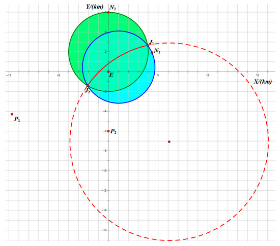
Figure 6.
The interception point in the non-degenerate scenarios.
5. Orbital Three-Versus-One Pursuit–Evasion Game
Consider a game with three pursuers () and one evader (). Following the same methodology, we set as the reference satellite in the relative coordinate system. Define as the interception domains determined by (), (), and (), with boundaries , respectively. Analogously, define the interception points in a one-versus-one game as .
Since all contain the origin, if any domain is nested within another, the game degenerates to one with fewer pursuers. Thus, we consider only the case where the three interception domains pairwise intersect (as shown in Figure 7, , and are shown by blue, green and red regions respectively). Denote at points , at points , and at points . The arc segments (defined in the previous section) are indicated by red dashed lines. The intersection region of is denoted as . Similarly, the interception point in must satisfy
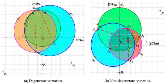
Figure 7.
Sketch of interception domains in three-versus-one pursuit–evasion game.
We first perform degeneracy determination based on initial states. The variety and complexity of cases here far exceed those in two-versus-one pursuit–evasion games. We initially divide them into degenerate and non-degenerate scenarios, then categorize the equilibrium interception points under both scenarios.
As shown in Table 2, degenerate scenarios can be classified into two types according to whether the game degenerates into a one-versus-one game or a two-versus-one game. If two equilibrium interception points from degenerate games coexist in , the point with the longer interception time must lie within the interception domain of the other degenerate game. This contradicts the definition of the equilibrium with the shorter interception time. Therefore, these two types are mutually exclusive, and the corresponding degenerate game is unique.
Table 2.
Two types of the degenerate scenarios in three-versus-one game.
Note that Figure 7a is a Type II degenerate scenario since . The initial states and game equilibrium in Figure 7b are presented in Section 7.3. In addition, if any interception domain contains another (e.g., ), the pursuer corresponding to the containing domain does not affect the game outcome. Such scenarios are necessarily degenerate scenarios.
Based on the above analysis, we summarize the algorithm for determining degeneracy and solving degenerate scenarios in three-vs.-one games as follows:
- Solve the Nash equilibrium for the one-vs.-one games between , , and , obtaining interception points and interception times . Compare . Assume without loss of generality.
- Compute , , and . Check if both and hold. If true, the game is a Type I degenerate scenario: intercepts at . Else, proceed.
- If , compute the interception point and interception time for the non-degenerate two-vs.-one game defined by . Similarly, if , compute and for . If , compute and for .
- For each computed in Step 3, determine (where is the third pursuer). If any , the game is a Type II degenerate scenario: and intercept at . Otherwise, the game is non-degenerate.
The above algorithm for degeneracy determination in the three-versus-one pursuit–evasion game requires solving three 16-dimensional TPBVPs in the first step, three 8-dimensional TPBVPs in the second step, and up to three additional 8-dimensional TPBVPs in the fourth step. The overall computational complexity is . When and , the total computation time typically ranges between 0.1 and 0.15 s. The decision tree presented in Steps 1–4 is summarized in Figure 8.
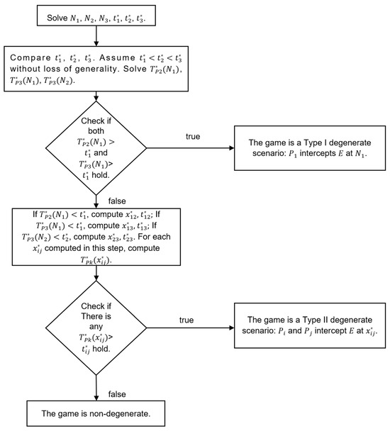
Figure 8.
Decision tree for determining degeneracy.
Due to the extreme complexity of classifying non-degenerate scenarios, we forgo rigorously characterizing equilibrium interception points. Instead, we identify candidate points for verification. Without loss of generality, assume the maneuver accelerations of the three pursuers satisfy . Thus, we can define the interception domains , , for pairs , , and . Note that intersection points of and satisfy and must lie on the boundary of . Thus, , , and intersect at two points and . By definition, if , they must be intersection points of the arcs , , and .
Theorem 3.
In the non-degenerate scenarios of a three-vs.-one game, only two types of equilibrium exist:
Type I: The interception point is located at pairwise intersection points of : .
Type II: The interception point is located at intersection points of .
Proof.
First consider the boundary of . Similar to the proof of Theorem 2.(1), the interception point cannot lie strictly within any interior segment of ; thus, only pairwise intersections are candidate points.
Next, consider the interior of . Analogous to Theorem 2.(2), any candidate point must satisfy . If the interception point satisfied , is the point with the longest interception time within its neighborhood in . However, this point must be , leading to a contradiction. Therefore, must satisfy .
By the equivalent definition of the interception domain, the set of points where must lie on the boundary of the domain , and similarly, points satisfying must lie on the boundary of . Therefore, any point satisfying must lie simultaneously on the boundary of and the boundary of . By definition, the intersection of the two boundaries is exactly the set . □
In the Type I non-degenerate scenario, although only two pursuers simultaneously intercept the evader, the presence of the third pursuer influences the evader’s strategy, resulting in an interception time shorter than in a game with only the other two pursuers. In the Type II non-degenerate scenario, all three pursuers intercept the evader simultaneously.
The key to computing the three-versus-one game equilibrium of the non-degenerate scenario lies in calculating intersections of pairwise interception domains. As discussed in Section 3, the interception domain can be approximated by an Apollonius circle scaled according to the ratio of the players’ accelerations. Therefore, the method for computing interception domain intersections involves first solving for intersections of these Apollonius circles, then using a homotopy method to gradually reintroduce the effects of relative velocity and gravitational field. The specific algorithm steps are as follows:
- Calculate the equations of the two Apollonius circles based on the two sets of satellite initial positions and acceleration magnitudes, respectively. For initial positions and acceleration magnitudes (assume without loss of generality that ), the center of the corresponding Apollonius circle is , and the radius is . Calculate the intersection points of the two Apollonius circles, denoted as .
- Define the evaluation function , which represents the sum of absolute value of the shortest time difference for two pairs of the pursuer and the evader to reach point when the relative coordinate line angular velocity is and the pursuer’s initial velocity direction is . By definition, and are the zeros of . Using and as starting points for the interior-point algorithm, obtain two zeros of , denoted as and .
- Set the number of iteration steps , and sequentially calculate the two zeros of , , , . The two zeros of , denoted as and , are computed using and as starting points for the interior-point algorithm, respectively. Similarly, for , the two zeros of , denoted as and , are computed using and as starting points for the interior-point algorithm, respectively. The final two zeros of , denoted as and , are the intersection points of the two interception domains.
The above algorithm for computing interception domain intersections involves invoking the interior-point method times. Let denote the maximum number of iterations required by the interior-point solver. Each invocation requires solving up to sets of three four-dimensional TPBVPs. Thus, the overall computational complexity is . In this paper, each intermediate problem (for ) is solved using MATLAB 2022A’s fmincon routine with a step-size tolerance of and a constraint tolerance of . When , , and , the overall numerical error of the algorithm is in the order of . The total computation time ranges from 100 to 150 s.
Based on the aforementioned algorithm for solving intersections of pairwise interception domains, the algorithm for finding interception points in non-degenerate scenarios can be derived from Theorem 3. The specific steps are as follows:
- Calculate the intersections of pairwise interception domains (for and ), (for and ), and (for and ), as well as the intersection points of , , and . Compute the shortest arrival times for , and to these points.
- Determine whether these points lie within . This is equivalent to verifying whether they satisfy for
- For the points identified in Step 2 that lie within , return the point that maximizes for
The above algorithm for computing interception points in non-degenerate three-versus-one pursuit–evasion scenarios requires four invocations of the interception domain intersection algorithm. The overall computational complexity is . When , , and , the total computation time ranges approximately from 300 to 500 s.
Finally, we consider the trajectory determination in non-degenerate scenarios. For the Type I scenario, the evader and the two simultaneously intercepting pursuers follow their respective minimum-time trajectories to the interception point. The remaining pursuer also follows its minimum-time path to the interception point (though it does not arrive by the game’s conclusion). For the Type II scenario, all three pursuers follow minimum-time trajectories to the interception point. Here, the evader arrives earlier than required, so its trajectory is non-unique. In subsequent simulations, for demonstration purposes, we assume the evader first maintains no maneuver before switching to its minimum-time path to reach the interception point.
6. Orbital Multi-Versus-One Pursuit–Evasion Game
This section discusses pursuit–evasion games with pursuers. Analogous to Section 5, define interception domains for each pursuer and the evader , where , with their intersection denoted as . Define pairwise interception domains for , each determined by pursuers and . The interception point in must satisfy
Since the probability measure of three circular-approximating convex domains with overlapping areas intersecting at a single point in the plane is zero, we disregard the possibility of all sharing a common intersection point for . Consequently, simultaneous interception by all pursuers becomes impossible. The game equilibrium exhibits fundamentally distinct characteristics beyond this demarcation threshold, justifying our focus on as the critical boundary. Here, the value of the threshold is a consequence of the planar problem geometry. An analysis of the same game in three dimensions would likely yield a higher threshold, as the increased spatial dimensionality allows for more complex domain intersections.
As the number of pursuers increases, an intuitive trend emerges: the likelihood of degenerate scenarios rises significantly. In high probability, not all pursuers become involved in the game. Conversely, solving non-degenerate scenarios becomes more tractable, with the primary computational bottleneck shifting to degeneracy determination.
Theorem 4.
In multi-vs.-one pursuit–evasion games with pursuers, the interception point in non-degenerate scenarios can only lie at pairwise intersection points of interception domains .
Proof.
First, consider the boundary points of . Without loss of generality, assume the interception point is on the boundary segment of within but not the intersection point of interception domains. Then, . There exists a neighborhood of on within , which satisfies . Thus, according to (16), must be the point with the largest in this neighborhood. However, this point can only be . indicates that the game degenerates into a one-versus-one game defined by (), which leads to the contrary.
Next, consider the interior of . Without loss of generality, assume the interception point satisfies .
Assume . Since must have an ascending gradient at , there exists a neighboring point such that . Here, will be intercepted later at , contradicting optimality. Thus, must satisfy .
Assume there exists satisfies , where is the point with the longest interception time within its neighborhood in . However, this point must be , leading to a contradiction. Thus, an interior interception point would require . However, such a point cannot exist for due to its measure-zero probability. □
Based on Theorem 4, we derive the method for computing the interception point. Due to the extreme complexity of degeneracy determination, we provide an iterative decision framework instead of explicit computational rules. The algorithm proceeds as follows:
- Solve reduced games by removing each pursuer in turn, yielding games defined by . Check if their interception points lie in (equivalent to verifying ). If any interception point satisfies this, terminate: the game degenerates to this -pursuer scenario.
- If Step 1 does not terminate, the game is non-degenerate. Compute all pairwise intersections of . Calculate minimum times for and to reach these points.
- For intersections from Step 2, verify membership in (equivalent to .
- Among feasible intersections from Step 3, select the point maximizing .
The computational complexity of the above algorithm for solving interception points in pursuit–evasion games with pursuers is dominated by the computations of interception domain intersections. Therefore, the overall computational complexity is .
Upon determining the interception point, the trajectories of all players under game equilibrium are determined as their respective minimum-time paths to this point.
7. Simulation Example
To validate the algorithm’s efficacy, we simulate two two-vs.-one, three three-vs.-one, and one four-vs. one pursuit–evasion examples. Among them, two two-vs.-one examples are corresponding to the non-degenerate and degenerate scenarios in Section 4, respectively; three three-vs.-one examples are corresponding to the two types of non-degenerate scenarios and degenerate scenarios in Section 5, respectively.
In all scenarios, the evader (reference satellite) is assumed to be in a geostationary orbit with angular velocity , orbital radius , and Earth-centered inertial coordinates . To ensure pursuers’ initial states align with its normality, they are initialized on circular orbits in the same orbital plane. Consequently, their positions and velocities in the Earth-centered inertial frame satisfy
where is Earth’s gravitational parameter. In the following, we present the Nash equilibrium results of the proposed algorithm in this paper under the aforementioned assumptions across four mission scenarios.
To ensure the credibility of the simulation results, a validation strategy based on internal consistency is employed. The following checks are performed: (1) The simulations are indeed based on the CW dynamics stated in Equation (2). The trajectories of all agents are generated by integrating these equations using their optimal control laws derived from (4)–(7). (2) For non-degenerate cases, the simultaneous interception time of the pursuers must agree within a numerical tolerance (<0.1 s). (3) The value of the Hamiltonian is monitored within a numerical tolerance (<) throughout the trajectory.
7.1. Example 1
The initial states (position and velocity in the relative coordinate system) and maneuvering accelerations for both pursuers and the evader are provided in Table 3.
Table 3.
Initial states of the players in Example 1.
Figure 9 illustrates the interception domains for Example 1. The equilibrium trajectories of all players and the distances between each pursuer and the evader are shown in Figure 10 and Figure 11, respectively. The results confirm that Example 1 represents a non-degenerate two-vs.-one pursuit–evasion scenario, where both pursuers simultaneously intercept the evader.
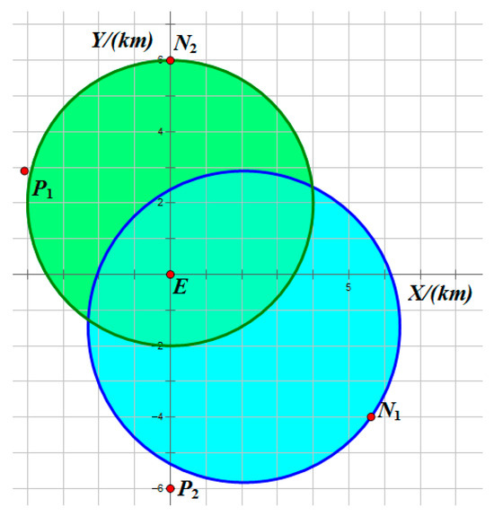
Figure 9.
Sketch of the interception domain in Example 1.
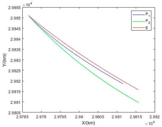
Figure 10.
Trajectories of the players in Example 1.
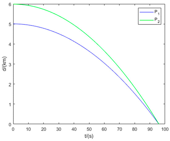
Figure 11.
Distance between the evader and the two pursuers in Example 1.
7.2. Example 2
The initial states and maneuvering accelerations for both pursuers and the evader are provided in Table 4.
Table 4.
Initial states of the players in Example 2.
Figure 12 illustrates the interception domains for Example 2. The equilibrium trajectories of all players and the distances between each pursuer and the evader are shown in Figure 13 and Figure 14, respectively. The results indicate that Example 2 represents a degenerate scenario in the two-vs.-one pursuit–evasion game. Only one pursuer intercepts the evader, while the other exerts no influence on the game outcome. Therefore, we assume that the non-participating pursuer executes no maneuver.
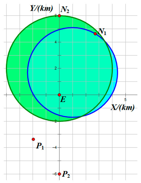
Figure 12.
Sketch of the interception domain in Example 2.
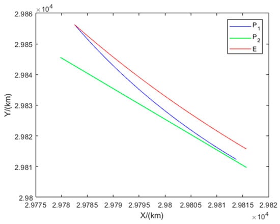
Figure 13.
Trajectories of the players in Example 2.
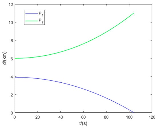
Figure 14.
Distance between the evader and the two pursuers in Example 2.
7.3. Example 3
The initial states and maneuvering accelerations for the three pursuers and the evader are provided in Table 5.
Table 5.
Initial states of the players in Example 3.
Figure 15 illustrates the interception domains for Example 3. The equilibrium trajectories of all players and the distances between each pursuer and the evader are shown in Figure 16 and Figure 17, respectively. The results show that Example 3 represents a Type I non-degenerate scenario in the three-vs.-one pursuit–evasion game, where the three pursuers simultaneously intercept the evader.
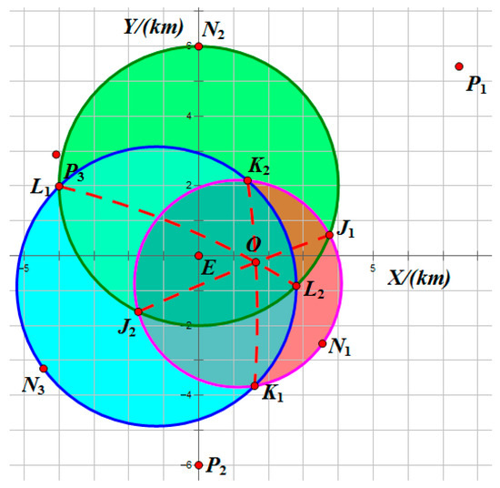
Figure 15.
Sketch of the interception domain in Example 3.
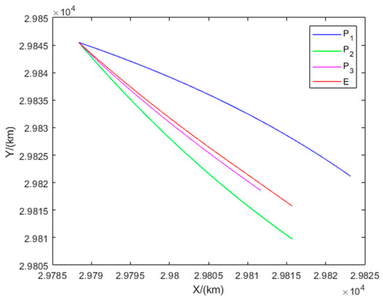
Figure 16.
Trajectories of the players in Example 3.
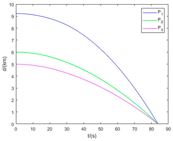
Figure 17.
Distance between the evader and the three pursuers in Example 3.
7.4. Example 4
The initial states and maneuvering accelerations for the three pursuers and the evader are provided in Table 6.
Table 6.
Initial states of the players in Example 4.
Figure 18 illustrates the interception domains for Example 4. The equilibrium trajectories of all players and the distances between each pursuer and the evader are shown in Figure 19 and Figure 20, respectively. The results show that Example 4 represents a Type II non-degenerate scenario in the three-vs.-one pursuit–evasion game, where under the strategic constraint imposed by the pursuer limiting the evader’s maneuverability, the remaining two pursuers , achieve simultaneous interception of the evader.
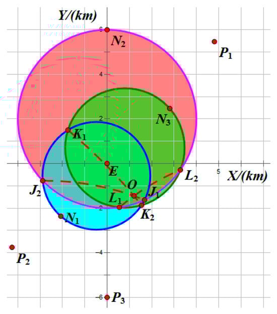
Figure 18.
Sketch of the interception domain in Example 4.
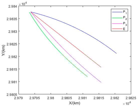
Figure 19.
Trajectories of the players in Example 4.
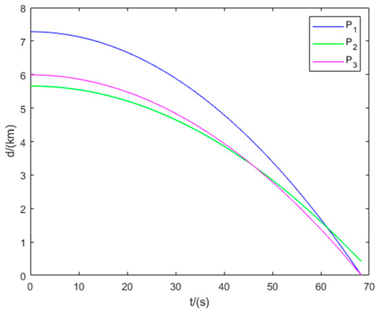
Figure 20.
Distance between the evader and the three pursuers in Example 4.
7.5. Example 5
The initial states and maneuvering accelerations for the three pursuers and the evader are provided in Table 7.
Table 7.
Initial states of the players in Example 5.
Figure 21 illustrates the interception domains for Example 5. The equilibrium trajectories of all players and the distances between each pursuer and the evader are shown in Figure 22 and Figure 23, respectively. Note that the initial states of Example 5 are the same as that of Example 3. However, the difference in maneuvering accelerations results in a degenerate scenario: exerts no influence on the game outcome, while and simultaneously intercept the evader.
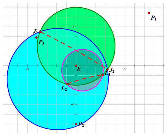
Figure 21.
Sketch of the interception domain in Example 5.
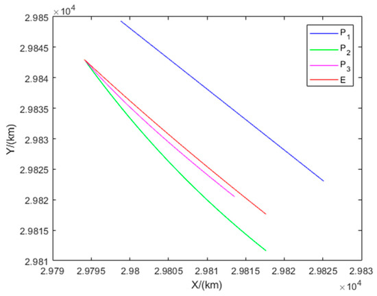
Figure 22.
Trajectories of the players in Example 5.

Figure 23.
Distance between the evader and the three pursuers in Example 5.
7.6. Example 6
The initial states and maneuvering accelerations for the three pursuers and the evader are provided in Table 8.
Table 8.
Initial states of the players in Example 6.
Through numerical computation, we have determined that the three-versus-one pursuit–evasion game defined by constitutes a non-degenerate scenario in which all three pursuers simultaneously intercept the evader. The interception point satisfies . This indicates that does not participate in the game. Therefore, the overall game degenerates to a three-pursuer engagement. Specifically, it corresponds to the Type I non-degenerate scenario as described in Section 5. The equilibrium trajectories of all players and the distances between each pursuer and the evader are shown in Figure 24 and Figure 25, respectively.
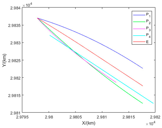
Figure 24.
Trajectories of the players in Example 6.
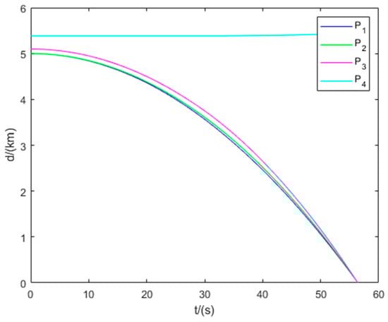
Figure 25.
Distance between the evader and the three pursuers in Example 6.
On the other hand, as analyzed in Section 5 regarding the computational load of the algorithm, the primary computational cost of our method stems from the homotopy iteration over initial velocities. However, since the relative initial velocity in Example 6 is zero, this step was unnecessary, resulting in a significantly reduced computation time of approximately 12.6 s for this specific example—far less than that required by the reachable set algorithm of Jansson and Harris [25] for a similar scenario. Although the computational performance of their method under non-zero initial velocity remains unclear, this result demonstrates that our algorithm holds a computational efficiency advantage in scenarios with small relative initial velocities.
8. Conclusions
This paper establishes the interception domain theory and applies it to planar orbital multi-player “encirclement-capture” differential games. The main contributions are as follows:
- We propose the first rigorous definition of interception domains for orbital pursuit–evasion games, prove their convexity, and develop computational methods for domain intersections. This theoretical framework enriches the methodological toolbox for orbital pursuit–evasion problems, providing a novel perspective for analyzing complex multi-spacecraft interactions.
- Based on this theoretical foundation, we establish a complete classification of equilibrium outcomes for planar multi-pursuer interception games. This classification exhibits a hierarchical structure as the number of pursuers increases: For , the solution degenerates to a single-pursuer interception, or both pursuers intercept simultaneously. For , in addition to the aforementioned outcomes, new equilibria emerge where the evader is intercepted simultaneously by all three pursuers, or by a pair of pursuers under the constraining influence of the third. For , our analysis proves that no more than three pursuers can simultaneously intercept the evader. The results reveal a phenomenon of diminishing returns beyond three pursuers, establishing that a three-pursuer configuration generally provides the most efficient resource utilization for planar orbital defense while maintaining strong interception efficiency.
- We analyze the Nash equilibrium properties for these games and develop efficient solution algorithms, including novel low-complexity methods for degeneracy determination. Compared to existing methods, our approach is particularly suitable for scenarios requiring rapid situation assessment.
Regarding the differential game model of orbital multi-player “encirclement-capture” games, several research directions warrant further investigation: First, while this work focuses on planar scenarios, the interception domain framework can be naturally extended to three-dimensional orbital environments. In such settings, the interception domain becomes a volume, and the critical number of pursuers required for simultaneous interception is expected to increase—a promising direction for future research. Second, the degeneracy determination method for large-scale pursuer scenarios remains complex. Future work should establish concise criteria for evaluating individual pursuers’ strategic influence. Finally, leveraging “encirclement-capture” solutions could optimize the configuration design (quantity/spatial deployment) of pursuers.
Author Contributions
Conceptualization, X.L.; formal analysis, G.Z.; investigation, X.L.; methodology, X.L.; resources, Y.L.; software, X.Y.; supervision, X.Z.; validation, X.Z.; writing—original draft, X.L. All authors have read and agreed to the published version of the manuscript.
Funding
This research received no external funding.
Data Availability Statement
Data is contained within the article.
Conflicts of Interest
The authors declare no conflicts of interest.
Abbreviations
The following abbreviations are used in this manuscript:
| TPBVP | Two-point boundary value problem |
| CW | Clohessy–Wiltshire |
| GEO | Geosynchronous Earth orbits |
Appendix A
The Apollonius circle is defined as the set of points in a plane with a constant ratio of distances to two fixed points:
When and , (A1) describes a circle.
In the orbital one-versus-one game governed by dynamics (2), if gravitational influence is neglected () and initial velocities are zero, the game reduces to a classical problem thoroughly analyzed in [2]. Under any boundary conditions specified in (7), the acceleration directions of and remain constant in the Nash equilibrium. Consequently, every point on the interception domain boundary satisfies
where is the time for both players to reach the point simultaneously. Given , the interception domain is an Apollonius circle containing scaled according to the ratio of the players’ accelerations.
Appendix B
The definitions of all points in sketches of the interception domain are as follows.
Table A1.
Definitions of all points in sketches of the interception domain.
Table A1.
Definitions of all points in sketches of the interception domain.
| Point | Definition |
|---|---|
| The initial position of in relative coordinate system. | |
| The initial position of in relative coordinate system. | |
| The initial position of in relative coordinate system. | |
| The initial position of in relative coordinate system. | |
| The interception point in one-versus-one pursuit–evasion game between and . | |
| The interception point in one-versus-one pursuit–evasion game between and . | |
| The intersection points of and . | |
| The intersection points of and . | |
| The intersection points of and . | |
| The intersection points of , and . |
References
References
- Anderson, G.M.; Grazier, V.W. Barrier in Pursuit-Evasion Problems Between Two Low-Thrust Orbital Spacecraft. AIAA J. 1976, 14, 158–163. [Google Scholar]
- Vajda, S.; Isaacs, R. Differential Games; Wiley: New York, NY, USA, 1965. [Google Scholar]
- Shen, H.X.; Casalino, L. Revisit of the Three-Dimensional Orbital Pursuit-Evasion Game. J. Guid. Control Dyn. 2018, 41, 1823–1831. [Google Scholar]
- Li, Z.Y.; Chen, S.; Zhou, C.; Sun, W. Orbital Multi-Player Pursuit-Evasion Game with Deep Reinforcement Learning. J. Astronaut. Sci. 2025, 72, 1. [Google Scholar]
- Pontani, M.; Conway, B.A. Numerical Solution of the Three-Dimensional Orbital Pursuit-Evasion Game. J. Guid. Control Dyn. 2009, 32, 474–487. [Google Scholar]
- Stupik, J.; Pontani, M.; Conway, B. Optimal Pursuit/Evasion Spacecraft Trajectories in the Hill Reference Frame. In Proceedings of the AIAA/AAS Astrodynamics Specialist Conference, Minneapolis, MN, USA, 13–16 August 2012; AIAA: Reston, VA, USA, 2012. [Google Scholar]
- Zhang, C.G.; Zhu, Y.W.; Yang, L.P. An Optimal Guidance Method for Free-Time Orbital Pursuit-Evasion Game. J. Syst. Eng. Electron. 2022, 33, 1294–1308. [Google Scholar]
- Zhou, J.F.; Zhao, L.; Li, H.; Cheng, J.H.; Wang, S. Compensation Control Strategy for Orbital Pursuit-Evasion Problem with Imperfect Information. Appl. Sci. 2020, 11, 1400. [Google Scholar] [CrossRef]
- Wang, Z.; Gong, B.; Yuan, Y.; Ding, X. Incomplete Information Pursuit-Evasion Game Control for a Space Non-Cooperative Target. Aerospace 2021, 8, 211. [Google Scholar] [CrossRef]
- Yang, B.; Liu, P.; Feng, J.; Li, S. Two-Stage Pursuit Strategy for Incomplete-Information Impulsive Space Pursuit-Evasion Mission Using Reinforcement Learning. Aerospace 2021, 8, 299. [Google Scholar] [CrossRef]
- Tang, X.; Ye, D.; Luo, S.; Low, K.-S.; Sun, Z. A Hybrid Game Strategy for the Pursuit of Out-of-Control Spacecraft under Incomplete-Information. Aerospace 2022, 9, 455. [Google Scholar] [CrossRef]
- Liu, P.; Yang, B.; Li, S.; Xin, M. Parameter-Optimized Pursuit Strategy for Orbital Games with Incomplete Information. J. Guid. Control Dyn. 2025, 48, 8. [Google Scholar]
- Li, Z.Y.; Zhu, H.; Yang, Z. Saddle Point of Orbital Pursuit-Evasion Game Under J2-Perturbed Dynamics. J. Guid. Control Dyn. 2020, 43, 1733–1739. [Google Scholar] [CrossRef]
- Wang, H.; Zhang, Y.; Liu, H.; Zhang, K. Impulsive thrust strategy for orbital pursuit-evasion games based on impulse-like constraint. Chin. J. Aeronaut. 2025, 38, 103180. [Google Scholar] [CrossRef]
- Han, H.; Dang, Z. Optimal delta-v-based strategies in orbital pursuit-evasion games. Adv. Space Res. 2023, 72, 243–256. [Google Scholar] [CrossRef]
- Ma, H.; Zhang, G. Delta-V analysis for impulsive orbital pursuit-evasion based on reachable domain coverage. Aerosp. Sci. Technol. 2024, 150, 109243. [Google Scholar] [CrossRef]
- Li, Z.Y.; Zhu, H.; Luo, Y.Z. Orbital Inspection Game Formulation and Epsilon-Nash Equilibrium Solution. J. Spacecr. Rockets 2024, 61, 157–172. [Google Scholar] [CrossRef]
- Wang, C.; Chen, D.; Liao, W. Research on Maneuver Strategy in Satellite Observation and Counter-Observation Game. Adv. Space Res. 2024, 74, 3170–3185. [Google Scholar] [CrossRef]
- Jagat, A.; Sinclair, A.J. Optimization of Spacecraft Pursuit-Evasion Game Trajectories in the Euler-Hill Reference Frame. In Proceedings of the AIAA/AAS Astrodynamics Specialist Conference, San Diego, CA, USA, 4–7 August 2014; AIAA: Reston, VA, USA, 2014. [Google Scholar]
- Jagat, A.; Sinclair, A.J. Nonlinear Control for Spacecraft Pursuit-Evasion Game Using the State-Dependent Riccati Equation Method. IEEE Trans. Aerosp. Electron. Syst. 2017, 53, 3032–3042. [Google Scholar]
- Ratnoo, A.; Shima, T. Guidance laws against defended aerial targets. In Proceedings of the AIAA Guidance, Navigation, and Control Conference, Portland, OR, USA, 8–11 August 2011. [Google Scholar]
- Li, Y.; Liang, X.; Dang, Z. Nash-equilibrium strategies of orbital Target-Attacker-Defender game with a non-maneuvering target. Chin. J. Aeronaut. 2024, 37, 365–379. [Google Scholar]
- Li, Z.-Y. Orbital Pursuit–Evasion–Defense Linear-Quadratic Differential Game. Aerospace 2024, 11, 443. [Google Scholar]
- Sun, S.; Zhu, H.; Wang, W. Orbital Three-Player Pursuit-Evasion Game. J. Astronaut. Sci. 2025, 72, 22. [Google Scholar] [CrossRef]
- Jansson, O.; Harris, M.W. A Geometrical, Reachable Set Approach for Constrained Pursuit–Evasion Games with Multiple Pursuers and Evaders. Aerospace 2023, 10, 477. [Google Scholar] [CrossRef]
- Jin, S.Y.; Qu, Z.H. Pursuit-Evasion Games with Multi-Pursuer vs. One Fast Evader. In Proceedings of the 2010 8th World Congress on Intelligent Control and Automation (WCICA), Jinan, China, 7–9 July 2010. [Google Scholar]
- Chen, J.; Zha, W.; Peng, Z.; Gu, D. Multi-player pursuit-evasion games with one superior evader. Automatica 2016, 71, 24–32. [Google Scholar] [CrossRef]
- Zhao, L.; Zhang, Y.; Dang, Z. PRD-MADDPG: An Efficient Learning-Based Algorithm for Orbital Pursuit-Evasion Game with Impulsive Maneuvers. Adv. Space Res. 2023, 72, 211–230. [Google Scholar] [CrossRef]
- Shinar, J. Solution techniques for realistic pursuit-evasion games. Control Dyn. Syst. 1981, 17, 63–124. [Google Scholar]
- Yan, R.; Shi, Z.; Zhong, Y. Reach-Avoid Games with Two Defenders and One Attacker: An Analytical Approach. IEEE Trans. Cybern. 2019, 49, 1035–1046. [Google Scholar] [CrossRef] [PubMed]
Disclaimer/Publisher’s Note: The statements, opinions and data contained in all publications are solely those of the individual author(s) and contributor(s) and not of MDPI and/or the editor(s). MDPI and/or the editor(s) disclaim responsibility for any injury to people or property resulting from any ideas, methods, instructions or products referred to in the content. |
© 2025 by the authors. Licensee MDPI, Basel, Switzerland. This article is an open access article distributed under the terms and conditions of the Creative Commons Attribution (CC BY) license (https://creativecommons.org/licenses/by/4.0/).