Physical Information-Based Mach Number Prediction and Model Migration in Continuous Wind Tunnels

Abstract

In wind tunnel tests for aerospace and bridge engineering, the accurate prediction of Mach number remains a core challenge to ensure the reliability of airflow dynamics characterization. Pure data-driven models often fail to meet high-precision prediction requirements due to the lack of physical mechanism constraints and insufficient generalization capability. This paper proposes a physical information-based long short-term memory network (P-LSTM), which constructs a physical loss function by embedding isentropic flow equations from gas dynamics, thereby constraining the Mach number prediction solution space within the physically feasible domain. This approach effectively balances the neural network’s ability to capture temporal features with the interpretability of physical mechanisms. Aiming at the scarcity of data in new wind tunnel scenarios, an adaptive weight transfer learning method (AWTL) is further proposed, realizing efficient knowledge transfer across different-scale wind tunnels via cross-domain data calibration, adaptive source-domain weight reweighting, and target-domain fine-tuning. Experimental results show that the P-LSTM method achieves a 50.65–62.54% reduction in RMSE, 48.00–54.05% in MAE, and 47.88–73.68% in MD compared with traditional LSTM for Mach number prediction in the 0.6 m continuous wind tunnel flow field. The AWTL model also outperforms the direct training model significantly in the 2.4 m continuous wind tunnel, with RMSE, MAE, and MD reduced by 85.26%, 95.12%, and 71.14%, respectively. These results validate that the proposed models achieve high-precision Mach number prediction with strong generalization capability.

1. Introduction

Wind tunnels play an irreplaceable and crucial role in the development process of many fields, such as bridges [1], buildings [2], trains [3] and aerospace [4,5,6]. Wind tunnels are able to simulate different airflow conditions and provide a controlled experimental environment for researchers, allowing them to deeply investigate the aerodynamic properties of objects under the action of airflow. Wind tunnel experimentation occupies a critical position in investigating the fundamental mechanisms of airflow, verifying the accuracy of aerodynamic theoretical models, and validating computational predictions, and generating aerodynamic datasets for the research, development, and optimization of aircraft, missiles, and other vehicular systems. With the rapid advancement of novel aerospace vehicles, the demands on wind tunnel testing have become more sophisticated, rendering wind tunnels essential and indispensable experimental apparatuses for the investigation of aerodynamic characteristics in advanced vehicle design.

During the variable angle of attack phase of wind tunnel experiments, it is necessary to control the Mach number of the wind tunnel within a small margin of error. The industry still mainly uses various improved PID control methods [7,8,9]. However, traditional PID control methods cannot meet the extremely high accuracy required for the Mach number. Additionally, as science and technology progress, newly designed and constructed wind tunnels are becoming increasingly complex, and the time lag, nonlinearity, multimodality, and other properties of the flow field inside the wind tunnel are becoming more prominent. Additionally, wind tunnel systems face challenges such as high modeling complexity, errors in Mach number measurement, and difficulty acquiring process variables.

In the performance evaluation system of wind tunnels, the Mach number has a central position, and its main task is to ensure that the air velocity in the wind tunnel is stabilized at a predetermined value of Mach number through the control system, so as to realize the precise regulation of the test conditions. However, stabilizing the Mach number is influenced by many complex factors. First, the wind tunnel model must accurately reproduce the actual working conditions. Nevertheless, different wind tunnel systems have unique operating characteristics due to differences in design parameters and application scenarios, making it difficult to generalize the modeling approach. Even within the same wind tunnel, the system characteristics change due to the diversity of purposes and dynamic changes in operating conditions, further increasing the complexity and difficulty of modeling. A more direct approach is predicated on data processing and mining.

The concept of wind tunnel predictive modeling was first introduced in 1984 when A. Manitius developed a Mach number prediction model for the second throat of a wind tunnel using system identification theory [10]. This model was integrated into the control system as a control object, achieving accurate prediction and control of wind tunnel performance. Ouyang J [11] achieved efficient prediction and analysis of wind tunnel aerodynamic data by establishing a back-propagation neural network model. This model used transonic and subsonic wind tunnel experimental data for training and was optimized using the LM technique. Wang S [12] based an improved feature subset integration (MFSE) method on multivariate fuzzy Taylor’s theorem to achieve high-precision, high-generalization prediction of the Mach number under large-scale, high-dimensional data in wind tunnel systems. Chen J [13] proposed a new method for high-precision Mach number prediction. This method addresses the ensemble prediction model’s poor accuracy, emphasizing fusion to enhance accuracy. Currently, data-based modeling approaches are mainly used for wind tunnel prediction modeling. Although these approaches demonstrate good prediction performance on their respective datasets, they require a large amount of data due to the nature of black-box learning. Additionally, the interpretability of black-box models is often questioned, and their responses have been found to exceed physical possibilities. Additionally, when faced with sparse data scenarios, a lack of generalization ability often occurs due to a lack of physical mechanism constraints [14].

In recent years, the long short-term memory (LSTM) network, proposed by Hochreiter and Schmidhuber [15], has performed well in processing and predicting time series data, especially in tasks requiring memorization of long-distance dependent information. The LSTM is a modified version of the recurrent neural network (RNN) designed to address the vanishing or exploding gradient problems that conventional RNNs encounter when handling lengthy sequential data. However, this method suffers from two problems: a large amount of data is required for training, and the model is difficult to interpret. Therefore, this paper proposes a physical information-based long short-term memory network (P-LSTM), which combines the advantages of physics-based and data-driven modeling. The model’s interpretability is ensured by restricting the solution space to the physical boundary through the physical information network. Our model combines physical information with data-driven modeling to accurately predict the Mach number [14,16]. Notably, our model still exhibits good prediction accuracy when the amount of data is small.

In the field of aerospace and fluid dynamics research, wind tunnel testing, as the core means of obtaining aerodynamic data of aircraft, has always been a key factor restricting the efficiency and scale of research due to its high construction and operation costs. The construction of wind tunnel facilities requires huge investment, involving complex engineering design and equipment procurement; during operation, the energy consumption of wind tunnels is particularly prominent, and some large-scale wind tunnels even need to be equipped with dedicated power stations and water supply systems to ensure operation, and the cost of a single complete wind test can reach tens of thousands of dollars. At the same time, in order to comprehensively analyze the aerodynamic characteristics of the aircraft, it is necessary to carry out systematic tests under multiple working conditions and parameters, so as to accumulate enough effective data for model construction and analysis. If tests and prediction models are conducted independently for each working condition, it will lead to a great consumption of resources and an exponential increase in cost. In addition, for new wind tunnels, even though their physical characteristics are similar to those of established wind tunnels, the initial test data are scarce, and reconstructing a new prediction model under such circumstances will not only lead to a waste of economic resources, but also make it difficult to satisfy the demand for rapid iteration of the research. Therefore, how to apply the existing wind tunnel test data and model results to new scenarios through model migration technology to realize the efficient reuse of data and knowledge has become an important issue that needs to be solved urgently.

Within the realm of artificial intelligence and machine learning, model migration emerges as a pivotal technical strategy, referring to the process of migrating a model trained in one domain to another related domain. This approach utilizes existing knowledge and experience to facilitate the rapid learning process of the new task, thereby reducing the necessity for substantial amounts of domain-specific data and enhancing the model’s adaptability and performance in its novel domain. For example, Guo J et al. [17] investigated the characteristic similarity between source and target domain data in predicting the travel time of China–Europe liner trains. They combined the data of the old process and realized the accurate prediction of the new process. Kang S et al. [18] utilized model migration to predict the service life of rolling bearings. Raykar et al. [19] proposed a Bayesian multi-instance learning method in which the method not only automatically performs feature selection, but also implements inductive migration, which is particularly useful for dealing with datasets with multiple instances and categories. Li L et al. [20] addressed the issue of near-infrared spectroscopy inter-instrument consistency leading to the problem of insufficient accuracy of the master model predicting spectra of slave instruments and proposed the transfer component analysis direct normalization (TCADS) algorithm, which combines nonlinear and linear corrections to effectively reduce spectral discrepancies and improve the performance of model migration. Zhao L et al. [21] proposed the input–output slope/bias correction-genetic algorithm (IOSBC-GA) model migration method. The model migration was achieved with a small amount of data by determining the model order through FNN, achieving nonlinear fitting through Elman network, and optimizing the migration parameters using GA. However, this method is only applicable to neural networks such as BP, RBF, etc., whose weight matrices can be optimized by linear offset technique. As for neural networks such as RNN, LSTM, etc., their parameters have wide diversity and the linear compensation method cannot optimize their performance effectively. For the mentioned neural networks, a universally effective model migration method has not been developed yet.

To address the limitations of existing model migration techniques, a data-driven adaptive weight model migration method (AWTL) is proposed in this paper. The method is composed of four core modules: similarity analysis, cross-domain data calibration, dynamic adjustment of source-domain sample weights, and target domain refinement training:

• Similarity analysis: In this study, the Euclidean distance is used as a measure of similarity between legacy and new conditions, and the historical conditions that are closest to the new conditions are filtered by calculating the distance value, thus supporting the construction and optimization of the model.
• Cross-domain data calibration module: Data distribution discrepancies between the source and target domains are systematically eliminated by constructing standardized conversion equations, establishing a unified data foundation for cross-domain knowledge migration.
• Source-domain sample weight dynamic adjustment mechanism: Based on the assessment of sample fitness to the target domain, source-domain samples are weighted using an adaptive weight allocation strategy, effectively suppressing noisy data interference and enhancing the migration efficiency of source-domain knowledge.
• Target domain refinement training strategy: A hybrid training dataset is constructed by fusing source-domain calibrated data and target-domain measured data, enabling the model to deeply adapt to target-domain data features while preserving effective source-domain knowledge.

Compared with traditional transfer learning methods, AWTL does not require complex modifications to network architectures and can be directly applied to mainstream deep learning models (e.g., RNN and LSTM). Through data-level optimization, this method provides an innovative solution for efficient migration of complex neural networks in cross-domain applications.

The remaining sections of this paper are structured around methodological construction and experimental validation, as follows: Section 2 elaborates on the P-LSTM model integrated with physical constraints and the adaptive weight transfer learning (AWTL) framework, detailing the modeling of a 0.6 m wind tunnel and the cross-domain migration strategy for a 2.4 m wind tunnel, respectively; Section 3 compares the model performance through multi-case experiments to verify the prediction accuracy and migration validity; and Section 4 summarizes the findings and makes recommendations for future research.

2. Materials

2.1. 0.6 m Continuous Wind Tunnel

Figure 1 shows the structural diagram of the 0.6 m continuous wind tunnel. This wind tunnel is a single-return configuration variable-density cryogenic continuous transonic wind tunnel, serving as a core piece of equipment for aerodynamic testing in the aerospace field, capable of supporting the verification of aerodynamic characteristics during the transonic phase of aircraft. In terms of structural design, a fully steel structure is adopted to ensure system stability. The test section dimensions are 0.6 m × 0.6 m × 2.7 m, providing ample space for model testing. In terms of operational parameters, the Mach number is adjustable within the range of 0.3 to 1.6, with a design pressure range of 0.02 to 0.4 MPa, enabling simulation of various atmospheric pressure conditions; the temperature regulation range is 233–333 K, meeting the requirements for variable density and temperature tests; the maximum Reynolds number reaches 8.17 × 10⁵.

The 0.6 m continuous wind tunnel serves as a key platform for simulating aerospace environments, based on a recirculating loop framework (ensuring continuous airflow circulation). It integrates a power system, cooling system, spray system, vacuum system, test section, measurement and control system, anti-icing air supply system, video surveillance system, and auxiliary equipment.

2.2. 2.4 m Continuous Wind Tunnel

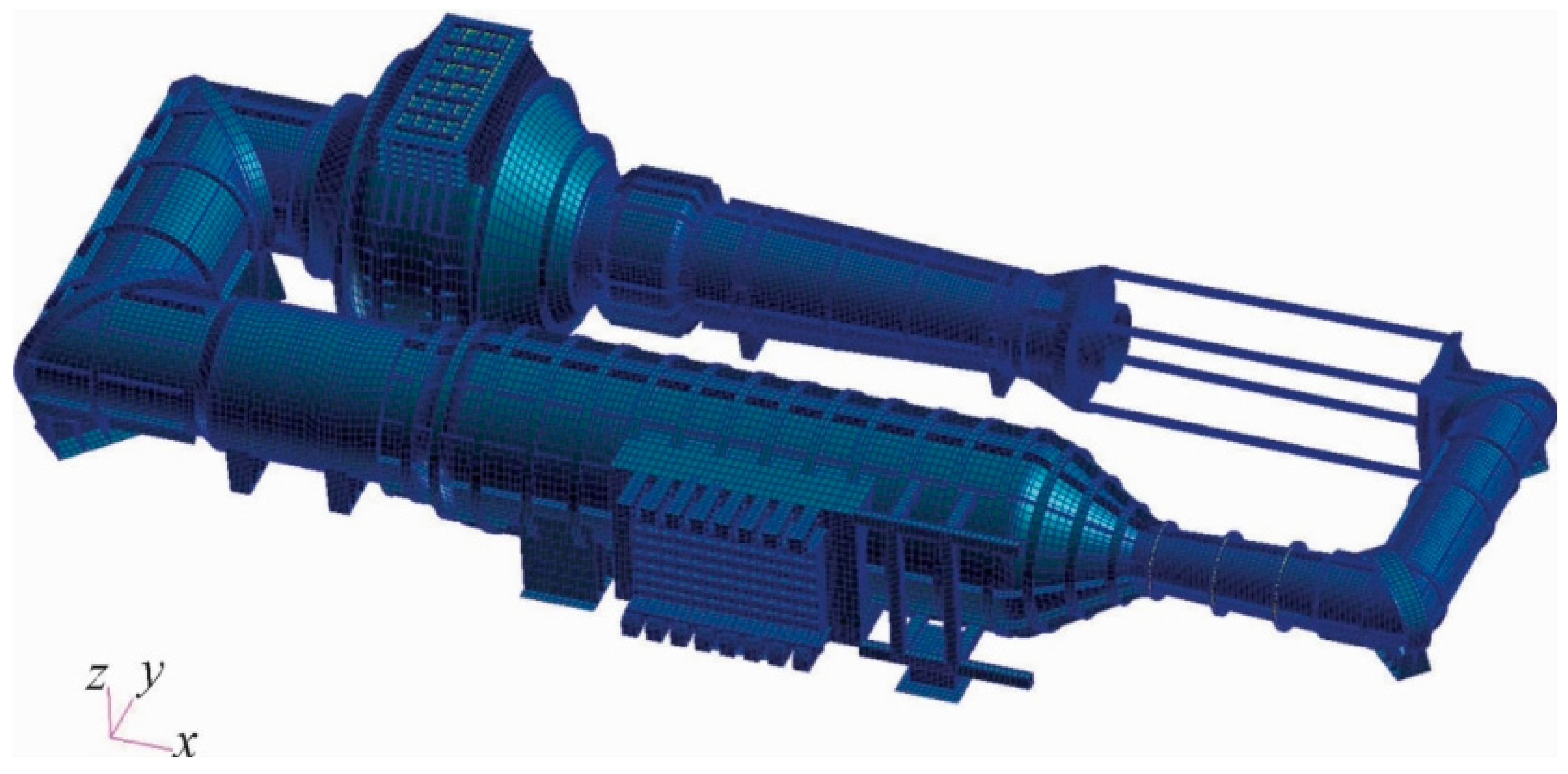
Figure 2 shows the 2.4 m continuous wind tunnel, with a test section size of 2.4 m × 2.4 m (cross-sectional dimensions), a Mach number adjustment range of 0.3 to 1.6, a total pressure control range of 0.03 to 0.4 MPa, a total temperature range of 293 to 333 K, and a maximum Reynolds number of 1.3 × 10⁷. This wind tunnel operates in a continuous mode, capable of simulating wide-speed-range and high-Reynolds-number aerodynamic environments and can accommodate large-scale aircraft models. It is primarily used for testing and research on transonic aerodynamic characteristics verification and aerodynamic layout optimization of large aircraft.

The 2.4 m continuous wind tunnel consists of two parts: the main system and auxiliary systems. The main system employs advanced technologies such as a central body with two throat channels, semi-flexible wall nozzles, a chamber isolation door, and a bypass loop, enabling rapid establishment of supersonic flow fields, replacement of test components while the compressor is in an incomplete shutdown state, and continuous precise control of the Mach number. The auxiliary systems include the chamber exhaust system, circulating water cooling system, air supply and exhaust system, high-pressure air supply system, and measurement and control system, which collectively ensure the stable operation of the wind tunnel.

3. Methodology

3.1. Mach Number Prediction for 0.6 m Continuous Wind Tunnel

In the study of Mach number prediction in a 0.6 m continuous wind tunnel (CWT), this paper first determines the input and output parameters of the model. Then, due to the limitations of the traditional LSTM model in capturing the characteristics of the Mach number sequence, a P-LSTM model is proposed to integrate the physical loss function into the two-layer LSTM architecture. Finally, three evaluation indexes are proposed to verify the accuracy of the model prediction.

3.1.1. Determine Inputs and Outputs

As mentioned above, the core objective of a wind tunnel control system is to achieve stable control of Mach number. In most studies, Mach number is typically used as the model’s output variable to illustrate the fitting effect. This study focuses on CWT Mach number characterization, which is set as the core predictor variable. In view of the dynamic evolution of Mach number, there is a significant temporal correlation between the current state and the predicted value in the future, which provides an important basis for the modeling and control strategy design in this study.

The operating conditions of a CWT are affected by the coupling of multiple variables, and the dynamic changes in each parameter will directly affect the output characteristics of the model. After analyzing the aerodynamic structure and process sequence of the wind tunnel, it can be seen that the main control variable is the fan speed (Fp), while the model angle of attack (An) exists as a disturbance quantity. For the flow field system, the Mach number (Ma) of the test section is the core control variable, and its dynamic characteristics are mainly governed by the coupling of the total pressure (P₀) of the stabilized section and the static pressure (P) of the test section. In this experiment, the temperature range was small and the measurement accuracy was limited, so we did not include temperature as an input in the model for now. The physical concepts of each variable are as follows:

(1)

Mach number (Ma):

The Mach number is a core dimensionless parameter in fluid dynamics that characterizes the ratio of fluid flow velocity to the speed of sound in a medium. It is named in honor of the Austrian physicist, Ernst Mach. In a wind tunnel experimental system, the Mach number is the primary control parameter used to regulate the experimental conditions. By precisely adjusting the airflow velocity, the complex flow field environment of an aircraft at different flight speeds can be effectively reproduced.

(2)

Fan speed (Fp):

In a continuous wind tunnel, the fan is one of the core drive components, whose function is to draw in air and create a directed airflow, which is then conveyed through ducts to the wind tunnel test section. The fan’s rotational speed directly affects the speed and stability of the airflow within the wind tunnel: the higher the rotational speed, the stronger the airflow’s driving capability, and the higher the airflow speed achievable in the test section. Therefore, by adjusting the fan’s rotational speed, the airflow speed within the wind tunnel can be precisely controlled to meet the requirements of different test conditions. In wind tunnel tests, the angle of attack is defined as the angle between the model’s reference axis and the freestream velocity vector.

(3)

Model angle of attack (An):

In wind tunnel tests, the angle of attack is defined as the angle between the model’s reference axis and the freestream velocity vector. In the phase of variable angle of attack test, the model angle of attack needs to be adjusted gradually to evaluate the aerodynamic characteristics after the wind tunnel Mach number is stabilized, during which the flow field inevitably generates perturbations, which leads to the challenge of Mach number stability. Research indicates that as the angle of attack shifts from a negative value up to zero degrees, the flow’s Mach number tends to rise. Conversely, when the angle is further increased from zero to positive degrees, the Mach number of the airflow correspondingly diminishes [22]. However, it should be noted that this trend typically applies to models without horizontal plane symmetry. For models with horizontal plane symmetry, this relationship will not hold.

(4)

Total pressure (P0) and static pressure (P):

The Mach number is significantly influenced by both total pressure and static pressure. Figure 3 illustrates the relationship between total pressure and static pressure. The total pressure is defined as the theoretical pressure of the gas flow when it is stagnant to zero velocity in an isentropic adiabatic process, and its magnitude is equal to the sum of the static and dynamic pressures of the gas flow, which is usually measured in the stabilization section of wind tunnels, while the static pressure refers to the pressure component perpendicular to the direction of the flow, and the data collection is performed in the test section. There is a clear coupling between the two and the Mach number: the total pressure can be independently adjusted, but its fluctuation will directly trigger the change in the Mach number, and vice versa; when the total pressure is maintained at a constant level, the static pressure becomes the dominant parameter in the regulation of the Mach number.

Figure 3. Schematic diagram of the physical significance of total pressure and static pressure.

Figure 3. Schematic diagram of the physical significance of total pressure and static pressure.

3.1.2. Long Short-Term Memory Networks (LSTM)

Mach number data exhibit significant time-sequence dynamics, and their evolution process depends not only on the current state of the system, but also on historical data, implying complex long-term dependencies. These characteristics require more advanced modeling methods that can handle long series data and capture long-term dependence information.

LSTM networks excel at sequence-to-sequence modeling. They have a unique recurrent connectivity mechanism that continuously retains historical information during the learning process. This allows them to effectively utilize previously learned knowledge of sequence data to predict the next state.

Figure 4 illustrates a simplified LSTM network architecture. A standard LSTM architecture is built around three core components: an input layer, one or more hidden layers, and a final output layer. While “LSTM” technically describes the entire neural network structure, it is commonly used to refer to individual layers or even the specialized memory cells within them. The network processes sequential data by transforming an input at time τ into a corresponding output at the same timestep (where τ ranges from 1 to m), which makes it particularly effective for sequence-to-sequence tasks. For proper functioning, both input and output data must be formatted as three-dimensional tensors. Dimension 1 is the time dimension, which characterizes the length of the sequence; dimension 2 is the batch dimension, which corresponds to the size of the batch or the number of data objects; and dimension 3 is the feature dimension, which consists of the input/output feature vectors.

The LSTM network is structured with multiple LSTM cells [23]. At the heart of an LSTM cell lies the cell state, serving as the main highway for information to flow across time steps with subtle interactions. Four key gates—forget, input, hyperbolic tangent (often called the candidate state), and output—work together to regulate this flow, enabling the network to retain or discard information as needed. These gates give the LSTM its cyclical nature and empower it to grasp intricate, time-dependent patterns within data. Among these, the forgetting gate removes unnecessary information, the input gate and hyperbolic tangent layer filter inputs, and the output gate regulates outputs.

Figure 5 illustrates a single LSTM network cell. In the lth LSTM layer, the operation of each control gate can be represented by Equations (1)–(6), which have corresponding weights $W_{\alpha }^{(l)}$ and biases $b_{\alpha }^{(l)}$. Here, α = {f, i, c, o} corresponds to the f oblivion gates, the $i$ input gates, the $c$ hyperbolic tangent layer, and the $o$ output gate. The input is $X_t$, forgetting gate output is $f_t^{(l)}$, input gate output is $i_t^{(l)}$, hyperbolic tangent gate output is ${\tilde{c}}_t^{(l)}$, output gate output is $o_t^{(l)}$, cell state memory is $c_t^{(l)}$, and hidden state output is $h_t^{(l)}$.

$$f_t^{(l)}=\sigma \left(W_f^{(l)}·{[h_{t-1},X_t]}^{(l)}+b_f^{(l)}\right)$$

(1)

$$i_t^{(l)}=\sigma \left(W_i^{(l)}·{[h_{t-1},X_t]}^{(l)}+b_i^{(l)}\right)$$

(2)

$${\tilde{c}}_t^{(l)}=\tanh \left(W_c^{(l)}·{[h_{t-1},X_t]}^{(l)}+b_c^{(l)}\right)$$

(3)

$$o_t^{(l)}=\sigma \left(W_o^{(l)}·{[h_{t-1},X_t]}^{(l)}+b_o^{(l)}\right)$$

(4)

$$c_t^{(l)}=f_t^{(l)}*c_{t-1}^{(l)}+i_t^{(l)}*{\tilde{c}}_t^{(l)}$$

(5)

$$h_t^{(l)}=o_t^{(l)}*\tanh \left(c_t^{(l)}\right)$$

(6)

where $\sigma$ is the logistic sigmoid function, whose value range is between 0 and 1, and is often used to output probabilities or weights; tanh stands for the hyperbolic tangent function, which maps the data to the interval between −1 and 1, and realizes the normalization of the information; $*$ denotes the Hadamard product, which is the multiplication of the corresponding elements of the matrix.

As a key parameter of fluid dynamics, the Mach number is a time series with nonstationary and high-order nonlinear characteristics. These characteristics include fluctuations in working conditions, coupling of historical states, and noise interference. (LSTM) is well-suited to handle such data due to its gated loop architecture. The forget gate filters historical information and retains trend features, the input and update gates collaborate to filter data features and update the state to capture dynamic changes, and the output gate combines historical and current information to output the hidden state with long-term dependence. Compared to traditional models, LSTM’s gating mechanism can more accurately model the dynamics of Mach number series, guaranteeing high-precision predictions.

3.1.3. Physical Information-Based Long Short-Term Memory Network Model (P-LSTM)

Nonetheless, the conventional LSTM model exhibits notable limitations. Primarily, its reliance on data-driven modeling hinders the capture of underlying physical laws, leading to low interpretability of model predictions and the potential for prediction bias due to the oversight of physical constraints. Additionally, the absence of an explicit fusion mechanism for physical a priori knowledge and the incapacity to integrate the strengths of theoretical fluid dynamics models into the training process constrain the model’s generalizability in complex working conditions. The model’s capacity for generalization is constrained in complex working environments. In light of these observations, this paper puts forth a proposal for a novel model, termed the P-LSTM model, that aims to address the aforementioned limitations by integrating physical constraints with the deep learning architecture.

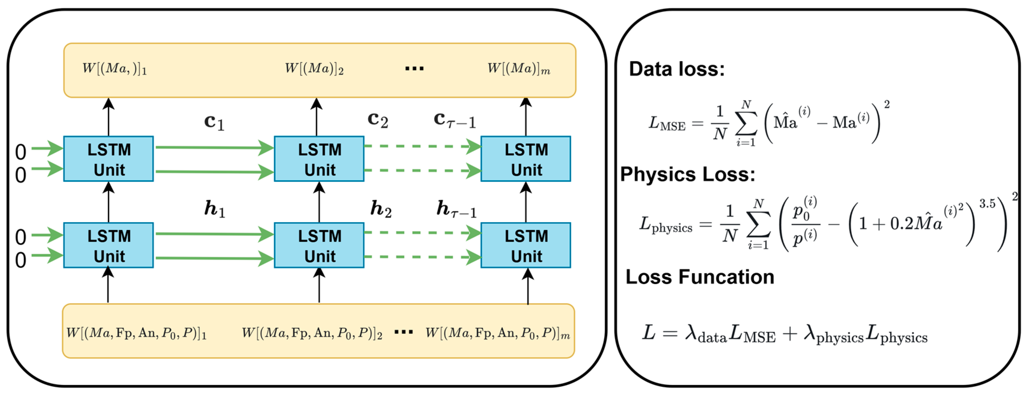
The P-LSTM architecture proposed in this paper represents an innovation over the traditional LSTM model by incorporating the laws of physics into the model [24]. This incorporation can significantly enhance prediction accuracy, interpretability, and generalization ability compared to a single data-driven time-series model. The LSTM network itself is analogous to the network architecture employed in traditional machine learning. As illustrated in Figure 6, the P-LSTM framework encompasses a comprehensive structure. The model’s distinguishing characteristic is that the weights and biases of the LSTM network are constrained by a physical loss function during training. This constraint ensures that the model predictions are consistent with the fundamental laws of gas dynamics and enhances interpretability. The P-LSTM network’s infrastructure remains consistent with that of a conventional model, thereby ensuring the capacity to efficiently model time-series data.

The P-LSTM model is composed of two LSTM layers, a structural element that facilitates the extraction of long-term dependent features and complex dynamic patterns in the data. The initial LSTM layer accepts the standardized historical data, including Mach number, fan speed, angle of attack, total pressure, and static pressure, as inputs. It then processes the timing information through the gating mechanism. The resulting output comprises the hidden state, cell state, and the intermediate feature information that is transmitted to the subsequent layer. The output layer of the second LSTM layer consists of a single node that outputs the predicted Mach number value.

In the P-LSTM framework, the loss computation combines elements of data-informed and physics-based losses. The data-informed part of the loss employs the mean square error (MSE) to gauge how far off the model’s forecasts are from the actual figures. This data-related loss is computed by Equation (7).

$$L_{\mathrm{MSE}}={\displaystyle \frac{1}{N}}{\displaystyle \sum _{i=1}^N{\left(\widehat{M}{a}^{(i)}-M{a}^{(i)}\right)}^2}$$

(7)

where N denotes the total number of samples, $\widehat{M}{a}^{(i)}$ represents the model’s Mach number prediction for the ith sample, and $M{a}^{(i)}$ indicates the actual Mach number value for that sample. This loss function encourages the model to capture temporal patterns and features within the data.

However, purely data-driven learning may have limitations. The model may overfit to noise in the data or produce predictions that violate physical laws under operating conditions not covered by the training samples. To address this issue, this paper introduces physical constraints based on the fundamental laws of gas dynamics, and the adiabatic flow equation serves as the core theoretical basis for constructing such constraints. The following derives the key formula for the ratio of total pressure to static pressure in adiabatic flow starting from the basic properties of calorically perfect gases, providing theoretical support for the construction of physical loss.

To study the flow of calorically perfect gases, it is first necessary to clarify their equation of state and the relationships between relevant thermodynamic parameters [25]. A calorically perfect gas satisfies the equation of state:

$$p=\rho RT$$

(8)

where $p$ is the static pressure, $\rho$ is the density, R is the gas constant, and T is the static temperature.

Meanwhile, there is a definite relationship between the specific heat at constant pressure c_p and the specific heat ratio $\gamma$:

$$c_p={\displaystyle \frac{\gamma R}{\gamma -1}}$$

(9)

Under steady, adiabatic, and inviscid flow conditions, the law of conservation of energy holds along a streamline. For any two points on the streamline, the sum of enthalpy and kinetic energy remains constant, i.e., the energy equation:

$$h_1+{\displaystyle \frac{u_1^2}{2}}=h_2+{\displaystyle \frac{u_2^2}{2}}$$

(10)

where h is the enthalpy and u is the flow velocity.

Since the enthalpy of a calorically perfect gas can be expressed as $h=c_{p}T$, the above energy equation can be transformed into a relationship between temperature and flow velocity:

$$c_p{T}_1+{\displaystyle \frac{u_1^2}{2}}=c_p{T}_2+{\displaystyle \frac{u_2^2}{2}}$$

(11)

To establish a connection between flow parameters and the stagnation state, the total temperature T₀ is defined as the temperature when the flow is isentropically stagnated to zero velocity, i.e., the temperature when the flow is hypothetically decelerated to rest adiabatically.

Based on the definition of total temperature, setting the flow velocity at a certain point u₂ = 0 in the energy equation, the corresponding temperature is the total temperature T₀, and the energy equation simplifies to

$$c_{p}T+{\displaystyle \frac{u^2}{2}}=c_p{T}_0$$

(12)

Through algebraic transformation, the ratio expression of total temperature to static temperature can be directly obtained:

$${\displaystyle \frac{T_0}{T}}=1+{\displaystyle \frac{u^2}{2c_{p}T}}$$

(13)

To enhance the practicality of the formula, it is necessary to establish a connection with the Mach number. According to the speed of sound formula $a=\sqrt{\gamma RT}$ and the definition of Mach number $Ma={\displaystyle \frac{u}{a}}$, combined with $c_p={\displaystyle \frac{\gamma R}{\gamma -1}}$, substituting into the above formula and simplifying yields the total temperature ratio formula:

$${\displaystyle \frac{T_0}{T}}=1+{\displaystyle \frac{\gamma -1}{2}}M{a}^2$$

(14)

This formula expresses the ratio of total temperature to static temperature in terms of Mach number and specific heat ratio. The total pressure $p_0$ is defined as the pressure when the flow is isentropically stagnated to zero velocity. In an isentropic process, there are definite relationships between the pressure, density, and temperature of a calorically perfect gas:

$${\displaystyle \frac{p_0}{p}}={\left({\displaystyle \frac{{\rho }_0}{\rho }}\right)}^{\gamma }={\left({\displaystyle \frac{T_0}{T}}\right)}^{{\displaystyle \frac{\gamma }{\gamma -1}}}$$

(15)

Since the relationship between the total temperature ratio and Mach number has been derived, substituting the total temperature ratio formula into the pressure–temperature relationship in the isentropic process establishes the connection between the ratio of total pressure to static pressure and Mach number:

$${\displaystyle \frac{p_0}{p}}={\left(1+{\displaystyle \frac{\gamma -1}{2}}M{a}^2\right)}^{{\displaystyle \frac{\gamma }{\gamma -1}}}$$

(16)

In summary, starting from the equation of state and energy equation of calorically perfect gases, by first defining total temperature and deriving its ratio relationship with static temperature, then utilizing the correlation characteristics between pressure and temperature in isentropic processes, the formula for the ratio of total pressure to static pressure in steady, adiabatic, and inviscid flow of calorically perfect gases is finally obtained:

$${\displaystyle \frac{p_0}{p}}={\left(1+{\displaystyle \frac{\gamma -1}{2}}M{a}^2\right)}^{{\displaystyle \frac{\gamma }{\gamma -1}}}$$

(17)

This formula indicates that the ratio of total pressure to static pressure depends solely on the Mach number Ma and the gas specific heat ratio $\gamma$. This study selects $\gamma$ = 1.4, a value widely recognized and adopted in engineering fields involving air flow such as aerospace and fluid machinery. It can well reflect the thermodynamic properties of air in compressible flow and ensure that the analysis and calculation results based on this formula have high consistency with actual flow conditions.

The core purpose of applying the adiabatic flow equation to the physical loss component is to introduce strict physical constraints into model predictions, ensuring that data-driven prediction results do not violate the basic laws of compressible flow. Relying solely on data-driven loss functions may lead to physically unreasonable prediction results—for example, contradictory situations where the Mach number does not match the ratio of total pressure to static pressure. As a fundamental law describing compressible flow, the adiabatic flow equation establishes a universal quantitative relationship between Mach number, total pressure, and static pressure. By embedding this equation into the physical loss component, the deviation between predicted values and theoretical physical laws can be quantified: when the total pressure/static pressure ratio calculated by substituting the Mach number output by the model into the formula is inconsistent with the actual measured value, the physical loss will increase significantly, thereby reversely correcting model parameters and forcing the prediction results to converge towards conforming to adiabatic flow laws. This constraint is particularly important in engineering scenarios. The physical loss component based on the adiabatic flow equation establishes a balance between data fitting and physical laws, improving the reliability and engineering applicability of model predictions. Its expression is

$$L_{\mathrm{physics}}={\displaystyle \frac{1}{N}}{\displaystyle \sum _{i=1}^N{\left(\frac{p_0^{(i)}}{p^{(i)}}-{\left(1+0.2\widehat{M}{a}^{{(i)}^2}\right)}^{3.5}\right)}^2}$$

(18)

where $p_0^{(i)}$ denotes the total pressure and $p^{(i)}$ denotes the static pressure of the ith sample. The Mach number $\widehat{M}{a}^{(i)}$ is predicted by the model. In instances where the predicted Mach number results in a deviation from the actual measured ratio of total pressure to static pressure, as indicated by the theoretical ratio, the value of the physical loss function is known to increase. This increase, in turn, prompts the model to adjust its parameters in order to satisfy the physical constraints.

Despite the demonstrated efficacy of constant weighting parameters in training physically informative neural networks, this paper proposes an adaptive rule, analogous to the one proposed by Wang S et al. [26], with the objective of enhancing the training process. The total loss function is expressed as a linear combination of the two losses previously defined, with the weights being adaptive and defined as follows:

$$L={\lambda }_{\mathrm{data}}{L}_{\mathrm{MSE}}+{\lambda }_{\mathrm{physics}}{L}_{\mathrm{physics}}$$

(19)

The adaptive weights are adjusted according to the dynamic changes in the two losses during the training process. Specifically, starting from the second training cycle, the Exponential Weighted Moving Average [27] is used to calculate the average of data loss and physical loss. This method gives higher weight to the recent losses and reflects the trend of losses in a more timely manner. The calculation formula is as follows:

$${\overline{L}}_{\mathrm{MSE}}^{(t)}=\alpha {\overline{L}}_{\mathrm{MSE}}^{(t-1)}+(1-\alpha )L_{\mathrm{MSE}}^{(t)}$$

(20)

$${\overline{L}}_{\mathrm{physics}}^{(t)}=\alpha {\overline{L}}_{\mathrm{physics}}^{(t-1)}+(1-\alpha )L_{\mathrm{physics}}^{(t)}$$

(21)

where $t$ denotes the training cycle, $\alpha$ is the smoothing coefficient (set to 0.5 in the experiments), ${\overline{L}}_{\mathrm{MSE}}^{(t)}$ and ${\overline{L}}_{\mathrm{physics}}^{(t)}$ are the moving averages of the data loss and the physical loss of the tth cycle, respectively. ${\overline{L}}_{\mathrm{MSE}}^{(t-1)}$ and ${\overline{L}}_{\mathrm{physics}}^{(t-1)}$ are the moving averages of the previous training cycle, which are initialized to the loss values of the first training cycle at the beginning of training.

The core idea of calculating the adaptive weights based on the average loss is to make the weights correlate with the inverse of the loss. The smaller the loss is, the better the model performs in that aspect, and the corresponding weight is larger to encourage the model to continue to maintain that advantage in subsequent training; conversely, the larger the loss is, the smaller the weight is. The specific calculation formula is as follows:

$${\lambda }_{\mathrm{data}}={\displaystyle \frac{1/({\overline{L}}_{\mathrm{MSE}})}{1/({\overline{L}}_{\mathrm{MSE}})+1/({\overline{L}}_{\mathrm{physics}})}}$$

(22)

$${\lambda }_{\mathrm{physics}}={\displaystyle \frac{1/({\overline{L}}_{\mathrm{physics}})}{1/({\overline{L}}_{\mathrm{MSE}})+1/({\overline{L}}_{\mathrm{physics}})}}$$

(23)

In this way, the sum of the two weights is always 1, which determines the contribution ratio of the data-driven loss and physical loss in the total loss function. At the same time, the model is able to dynamically balance the emphasis on data fitting and physical law following and gradually optimize the prediction performance during the training process to achieve highly accurate and physically realistic Mach number prediction.

3.1.4. Evaluating the Model

To gauge how well the proposed model performs in making predictions, three key metrics are employed: Root Mean Square Error (RMSE), Mean Absolute Error (MAE), and Maximum Deviation (MD). These are detailed in Equations (24)–(26) and collectively provide a well-rounded view of the prediction accuracy. While RMSE emphasizes larger errors, MAE offers an average deviation measure, and MD highlights the greatest single discrepancy, each capturing distinct facets of how predictions compare to real-world data.

$$\mathrm{RMSE}=\sqrt{{\displaystyle \frac{{\displaystyle \sum _{t=1}^N{({\widehat{y}}_t-y_t)}^2}}{N}}}$$

(24)

$$\mathrm{MAE}={\displaystyle \frac{1}{N}}{\displaystyle \sum _{t=1}^N|}{\widehat{y}}_t-y_t|$$

(25)

$$\mathrm{MD}=\max \left|y_t-{\widehat{y}}_t\right|$$

(26)

where ${\widehat{y}}_i$ denotes the predicted value of Mach number, $y_t$ denotes the actual value of Mach number, and N is the total number of predicted values. Specifically, lower values of RMSE, MAE, and MD are indicative of higher prediction accuracy, as they reflect a stronger correlation between the predicted values and the actual Mach number.

3.2. Mach Number Prediction for 2.4 m Continuous Wind Tunnel

The Mach number prediction model for a 0.6 m CWT was detailed earlier; however, the method still faces two major challenges in practical engineering applications: first, P-LSTM relies on a large amount of data to construct an accurate model, but the data collection under new working conditions is often limited by the cost and time of experiments; second, the model prediction accuracy decreases significantly when migrating the model from the source domain to the target domain due to the scaling effect of the fluid dynamics properties. Second, when directly migrating the source domain model to the target domain, the model prediction accuracy decreases significantly due to the scaling effect of fluid dynamics properties. Especially for the newly constructed 2.4 m CWT, although it follows the same physical laws as the 0.6 m CWT, the direct use of the 0.6 m model will introduce non-negligible systematic errors, and a complete remodeling will require a lot of manpower and financial resources. To address the above problems, this paper proposes an AWTL method, which aims to establish a descriptive model of the 2.4 m CWT using the established 0.6 m CWT model and limited new operational data from the 2.4 m CWT.

Aiming at the data-dependent and cross-domain migration accuracy attenuation difficulties facing the 2.4 m CWT Mach number prediction, this study proposes the adaptive weight migration learning modeling method. To begin, the system evaluates the resemblance between previous and current operating parameters by analyzing their data patterns, and the old operating conditions with high similarity are selected for model migration; then, the cross-domain data calibration is realized based on the statistical normalization to eliminate the distributional differences between the old working condition and new working condition; then, the adaptive weight migration strategy is used to dynamically adjust the weights of the source domain samples based on the individual migration errors, and the interference of the low-fit samples is suppressed; finally, the hybrid training method is constructed for the prediction of 2.4 m CWT Mach number. Finally, a hybrid training set with weight adjustment is constructed to integrate the calibrated source and target domain data as inputs to the P-LSTM model, which can effectively alleviate the problem of scarcity of data for new operating conditions and realize the migration of 2.4 m CWT Mach number prediction model.

3.2.1. Similarity Analysis

The accurate measurement of the similarity of the working conditions is a key aspect when performing model migration. In this study, the Euclidean distance method is used to measure the degree of similarity between the source and target domain data. The distance between the source and target domain data is calculated according to Equation (27).

$$d_i(D_i,D_{\mathrm{new}})=\Vert D_i-D_{\mathrm{new}}{\Vert }_2={\left({\displaystyle \sum _{k=1}^n}|d_{ik}-d_{\mathrm{new}k}{|}^2\right)}^{{\displaystyle \frac{1}{2}}}$$

(27)

where $D_i$ represents the first historical data, $D_{\mathrm{new}}$ is the new data, and n is the total number of feature sets. In order to achieve effective comparison between different samples, the above distance is further normalized and mapped to the interval [0, 1] to obtain the similarity index, which is calculated as shown in Equation (28):

$${\mathrm{sim}}_i(D_i,D_{\mathrm{new}})={\displaystyle \frac{1}{1+d_i(D_i,D_{\mathrm{new}})}}$$

(28)

Based on the above similarity calculation results, the historical working conditions that are most similar to the new working conditions are screened out, and the model is constructed based on this.

3.2.2. Cross-Domain Data Calibration

In the model migration task, there is often a significant distribution difference between the old working condition data (0.6 m CWT) and the new working condition data (2.4 m CWT). Due to the differences in data acquisition environment, equipment parameters, sample population and other factors, it is difficult to directly adapt the old working condition to the application scenarios in the new working condition. If the unprocessed old working condition data are directly used for model training, the model is prone to overfitting phenomenon and cannot effectively learn the features of the new working condition data, resulting in a significant decrease in the prediction accuracy in the new working condition. This makes it difficult for the model to achieve reliable prediction and analysis in real scenarios. Therefore, after selecting the best old working condition data, this paper first calibrates the old working condition data to make its distribution close to the new working condition and reduce the working condition differences, thereby reducing the domain discrepancy and laying a solid foundation for subsequent model training. The specific calibration process is as follows:

For the old working condition data $X_s\in R^{n_s\times d}$ and the training set new working condition data $X_t\in R^{n_t\times d}$, where $n_s$ and $n_t$ are the number of samples in the old working condition and new working condition, respectively, and $d$ are the feature dimensions. The statistics are first calculated based on the following equation:

$$\left\{\begin{array}{l}{\mu }_s={\displaystyle \frac{1}{n}}{\displaystyle \sum _{i=1}^n{x}_{s,i}},{\sigma }_s=\sqrt{{\displaystyle \frac{1}{n}}{\displaystyle \sum _{i=1}^n{(x_{s,i}-{\mu }_s)}^2}}\\ {\mu }_t={\displaystyle \frac{1}{m}}{\displaystyle \sum _{j=1}^m{x}_{t,j}},{\sigma }_t=\sqrt{{\displaystyle \frac{1}{m}}{\displaystyle \sum _{j=1}^m{(x_{t,j}-{\mu }_t)}^2}}\end{array}\right.$$

(29)

where ${\mu }_s,{\mu }_t$ are the vectors of old working condition data and new working condition data means, respectively, and ${\sigma }_s$, ${\sigma }_t$ are the vectors of standard deviation of old working condition data and new working condition data of the training set, respectively.

The calibration parameters $\mathsf{\alpha }$, $\mathsf{\beta }$ are calculated by the following equation:

$$\left\{\begin{array}{l}\mathsf{\alpha }={\displaystyle \frac{{\mathsf{\sigma }}_t}{{\mathsf{\sigma }}_s}}\hfill \\ \mathsf{\beta }={\mathsf{\mu }}_t-\mathsf{\alpha }{\mathsf{\mu }}_s\hfill \end{array}\right.$$

(30)

where ${\mathsf{\mu }}_s$, ${\mathsf{\sigma }}_s$ and ${\mathsf{\mu }}_t$, ${\mathsf{\sigma }}_t$ are the mean and standard deviation vectors of the data in the old working condition and the new working condition of the training set, respectively. The final calibrated old working condition data ${\widehat{X}}_s$ is

$${\widehat{X}}_s=X_s\mathsf{\alpha }+\mathsf{\beta }$$

(31)

By this method, the data distribution error between source and target domains is effectively reduced, and cross-domain data calibration from source to target domain is realized.

3.2.3. Source Domain Sample Weight Adjustment

Although data calibration across domains helps to minimize the disparity in data distribution between the source and target areas, certain samples in the source domain’s data still exhibit minimal relevance to the target domain, and these samples may introduce interference during the model training process, which affects the model’s learning of the target domain features. For this reason, this study proposes an AWTL method to achieve accurate optimization of source domain data by the following methods:

Firstly, the old working condition data weight vector $w_s=[w_s^1,w_s^2,\dots ,w_s^{n_s}]$ and the new working condition data weight vector $w_t=[w_t^1,w_t^2,\dots ,w_t^{n_t}]$ are given, and initially each source and target domain sample $x_s^i$ and $x_t^i$ is assigned an initial weight 1.

In order to reflect the fitness of the old working condition data to the old working condition model, this paper defines the individual migration error of the source domain sample i in the ( $k-1$)th iteration as

$$e_s^{(k-1),i}=\left|f^{(k-1)}(X_s^i)-y_s^i\right|$$

(32)

where $f^{(k-1)}$ is the model after the ( $k-1$)th round of training, $X_s^i\in R^{n_s\times d}$ is the source domain input data, and $y_s^i$ is the real Mach number label. The error directly reflects the fitness of the source domain samples to the target domain model: the smaller the error, the closer the distribution of sample features is to the target domain, and the higher the migration value.

At the same time, an exponential weighting strategy is introduced to dynamically adjust the weights of the old working condition data.

$$w_s^{(k),i}=w_s^{(k-1),i}·{\theta }^{e_s^{(k-1),i}}$$

(33)

where $\theta$ is the target domain sensitivity coefficient, defined as

$$\theta ={\displaystyle \frac{1}{1+{\overline{e}}_t^{(k-1)}}}$$

(34)

$${\overline{e}}_t^{(k-1)}={\displaystyle \frac{1}{N_t}}{\displaystyle \sum _{j=1}^{N_t}\left|f^{(k-1)}(X_t^j)-y_t^j\right|}$$

(35)

${\overline{e}}_t^{(k-1)}$ is the average absolute error of the target domain training set. When the target domain error ${\overline{e}}_t$ is large, $\theta$ is close to 0, and the weights of the low error source domain samples are significantly reduced; when ${\overline{e}}_t$ is large, $\theta$ is close to 1, and the weights are adjusted smoothly to prevent excessive perturbation of the learned target domain knowledge.

After each iteration, a weighted sampler is constructed based on the updated weights $w_s^{(k)}$ to resample the source domain samples. Samples with small errors are given higher sampling probabilities and are learned multiple times in subsequent training, while samples with large errors appear less frequently.

3.2.4. Target Domain Refinement Training

After cross-domain data calibration and source-domain sample weight adjustment, the source-domain data are optimized in terms of distribution characteristics and sample value screening, which lays a good foundation for model migration. However, to realize more efficient and accurate model migration, the target domain training process needs to be further fine-designed to fully integrate the advantages of source and target domain data. Therefore, on the basis of retaining the sample weight matrix in the source domain, this study carries out fine training in the target domain, aiming at constructing a better training system to improve the performance of the model in the target domain.

On the basis of retaining the source domain sample weight matrix $W_s^{(t)}\in R^{N_s\times 1}$ (where $N_s$ is the number of samples in the source domain and t is the number of iteration rounds), the target domain samples are given a uniform base weight ${\omega }_t=\alpha ·1_{N_t}$, $1_{N_t}$ is a $N_t$-dimensional all-1 vector, and $\alpha$ is the weight coefficient in the target domain, which can be adjusted according to the actual working conditions to adjust the ratio of weights in the target domain to those in the source domain. Through the design of the weighting system, a hybrid training set containing cross-domain calibrated source domain data $X_s$ and target domain measured data $X_t$ is constructed:

$${\mathcal{D}}_m={\left\{\left(X_s^{(i)},y_s^{(i)},w_s^{(i)}\right),\left(X_t^{(j)},y_t^{(j)},{\omega }_t\right)\right\}}_{i=1,j=1}^{N_s,N_t}$$

(36)

where $w_s^{(i)}$ is the dynamic weight of the ith source domain sample, $N^s$ is the number of source domain samples, $x_s^i$ is the feature vector of the ith sample in the target domain; $y_s^i$ is the label value of the ith target domain sample; ${\omega }_t$ is the target domain data weight, $N^t$ is the number of target domain samples, $x_t^j$ is the feature vector of the jth sample in the target domain; and $y_t^j$ is the label value of the jth target domain sample. Through the construction of this hybrid training set, on the one hand, the high-value data in the source domain after calibration and weight screening are deeply reused to give full play to its guiding role in feature migration; on the other hand, the measured data in the target domain is used as the core to ensure that the model can closely match the actual data characteristics and application requirements of the target domain.

Finally, the constructed merged training set ${\mathcal{D}}_m$ is used as the input data of the P-LSTM model. This study employs the outlined approach to augment target domain data, while leveraging source domain data to mitigate potential model overfitting issues stemming from limited target domain samples. By implementing a cross-domain knowledge transfer mechanism, the paper successfully achieves accurate Mach number predictions for the 2.4 m CWT case.

4. Illustration and Discussion

4.1. Selection of Experimental Conditions

The 0.6 m CWT and 2.4 m CWT studied in this thesis have carried out a series of variable angle of attack wind blowing tests in the previous period, accumulating a certain amount of test data. In the wind tunnel conditions studied in this paper, the ejection slit is set at 28 mm; the opening and closing ratio is set at 2%, and the total pressure is atmospheric. Among them, the 0.6 m CWT was designed and constructed earlier, and the test data are more sufficient, the data were selected under the condition that the wind tunnel’s Mach number was running stably while the angle of attack was changing, and three more typical working conditions were divided according to the needs. While the test data of 2.4 m CWT are relatively lacking, only one experimental working condition is listed in this thesis. The basic information on the working conditions is shown in

Table 1. Working conditions in a 0.6 m CWT.

Test Condition	Mach Number	Motor Speed Interval (r/s)	Angle of Attack (°)	Number of Samples
1	0.3	1000	−4–0	499
2	0.3	1000	−3–4	1064
3	0.8	1800	−2–2	765

and

Table 2. Working conditions in a 2.4 m CWT.

Test Condition	Mach Number	Motor Speed Interval (r/s)	Angle of Attack (°)	Number of Samples
1	0.9	350	0–4	1030

.

4.2. Parameter Selection

The identification of optimal hyperparameters within the test dataset to ensure maximized generalization capability plays a pivotal role in achieving highly precise predictive outcomes. The main influences on the prediction accuracy of a P-LSTM model include time step, batch size, and the number of LSTM neurons. If these parameters are set too high, the P-LSTM model may experience overfitting, while if these parameters are set too low, the model may exhibit underfitting. To ensure that the P-LSTM algorithm maintains good prediction accuracy and stability, determining the optimal values for the time step, batch size, and number of neurons is necessary.

Table 3. Comparison of evaluation metrics for P-LSTM models at different time steps.

Time Step	RMSE/10−5	MAE/10−5
5	8.21	6.44
10	21.15	12.32
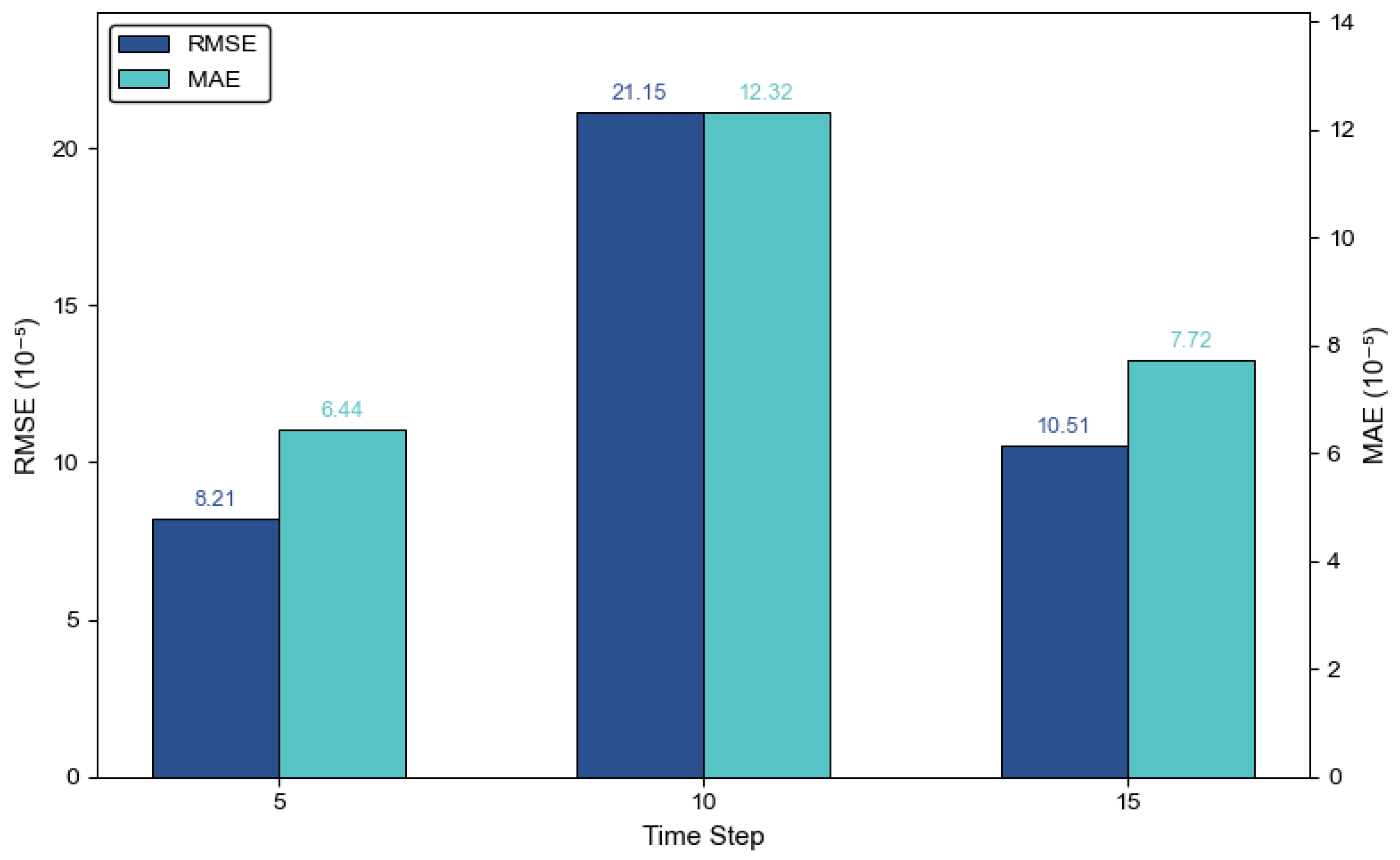
15	10.51	7.72

and Figure 7 demonstrate the prediction results of the P-LSTM model at different time steps. It is found that the time step size is not simply linearly related to the model prediction error. When the step size is small, increasing the order may lead to a significant increase in the prediction error, perhaps because too large a step size causes the model to overfit specific patterns in the training data and reduces the generalization ability, whereas continuing to increase the step size within a certain range decreases the error, implying that appropriately increasing the step size can help the model to better capture the long-term dependence features of the data. However, the process is highly complex, and either too high or too low a step size setting can adversely affect the model performance. Therefore, the optimal time step for the P-LSTM model in this study is set to 5.

In the hyperparameter optimization system of the P-LSTM model, batch size functions as the primary regulatory variable, with its value exerting a direct influence on the model’s training stability and prediction efficiency. This assertion is supported by the empirical data presented in

Table 4. Comparison of evaluation metrics for P-LSTM models at different batch size.

Batch Size	RMSE/10−5	MAE/10−5
16	8.06	6.32
32	8.21	6.44
64	10.25	7.63

. A systematic analysis of the two key indicators, RMSE and MAE, was conducted. The results of this analysis indicate that: An examination of the data reveals a weak, fluctuating tendency in the RMSE and MAE indicators when the batch size is increased from 16 to 32. This finding suggests that the effect of adjusting the batch size on the model’s performance is not significant within this range. Conversely, when the batch size is expanded to 64, the RMSE and MAE indicators demonstrate a substantial increase, indicating that the effect of adjusting the batch size on the model’s performance becomes significant at this point. As shown in Figure 8, the root RMSE and MAE metrics exhibit substantial increases. These results indicate that overly large batch sizes can cause the model to prioritize local data features, thereby diminishing its capacity to generalize to unseen data. Furthermore, large-batch training has been shown to increase the memory load and trigger a bottleneck in computational resources, which, in turn, reduces the efficiency and stability of the training process. In summary, under the present experimental conditions, when the batch size is set to 16, the P-LSTM model is able to achieve the optimal balance of RMSE and MAE metrics and shows the best prediction performance.

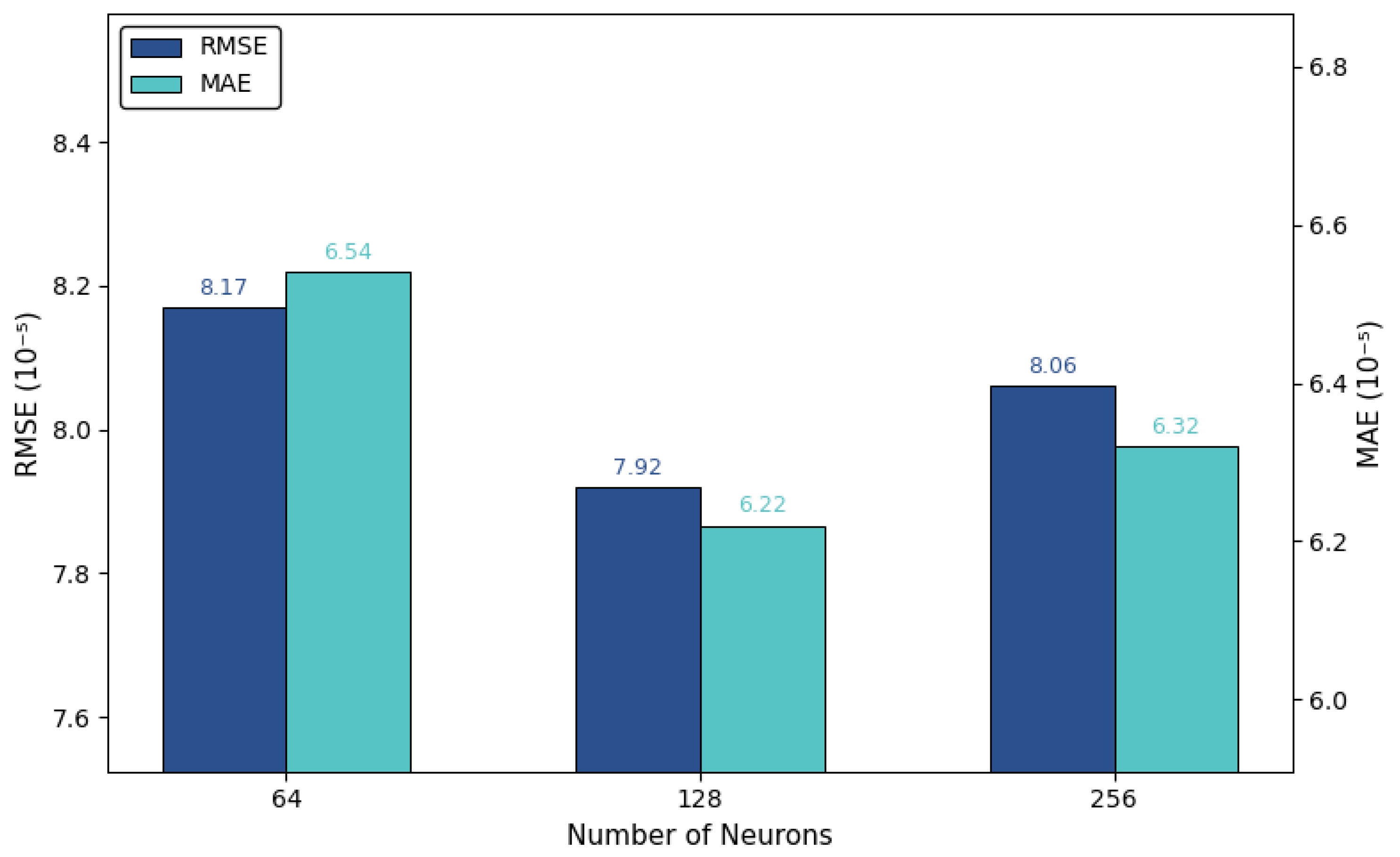
The number of LSTM neurons is also a key parameter that affects the performance of the model. As can be seen from the data in

Table 5. Comparison of evaluation metrics for P-LSTM models at different neurons.

Neurons	RMSE/10−5	MAE/10−5
64	8.17	6.54
128	7.92	6.22
256	8.06	6.32

and Figure 9, when the number of neurons is increased from 64 to 128, both the RMSE and MAE metrics decrease, indicating that the model’s ability to capture temporal features is enhanced and the prediction accuracy is improved; while the metrics rebound when the number is further increased to 256, indicating that the model may be slightly overfitted due to excess capacity. This trend reflects the balance between model complexity and generalization ability: a medium number of neurons 128 achieves a better balance between underfitting and overfitting, extracting effective features while avoiding noise interference. Therefore, the prediction performance of the P-LSTM model is better when the number of neurons is 128 under the conditions of this experiment.

After pinpointing the optimal settings for neurons, sequence arrangement, and batch size in the P-LSTM model. The model’s network parameters and architecture require further definition. In this study, a probabilistic search approach is employed to fine-tune the hyperparameters of the P-LSTM model.

Table 6. Hyperparameter settings for the P-LSTM model.

Neurons	Range	Value
Time step	[5, 10, 15]	5
Batch size	[16, 32, 64]	16
neurons	[64, 128, 256]	128
Learning rate	[0.1, 0.01, 0.001, 0.0001]	0.001
Optimizer	Adam, SGD, Adagrad, RMSProp	Adam
Epochs	[250, 300, 400, 500]	500

outlines the optimized settings, such as the number of training epochs, learning rate, batch size, as well as the input sequence length and the number of neurons in the network. This set of hyperparameters will be used in subsequent experiments.

4.3. Experimental Results

4.3.1. 0.6 m CWT Experiments

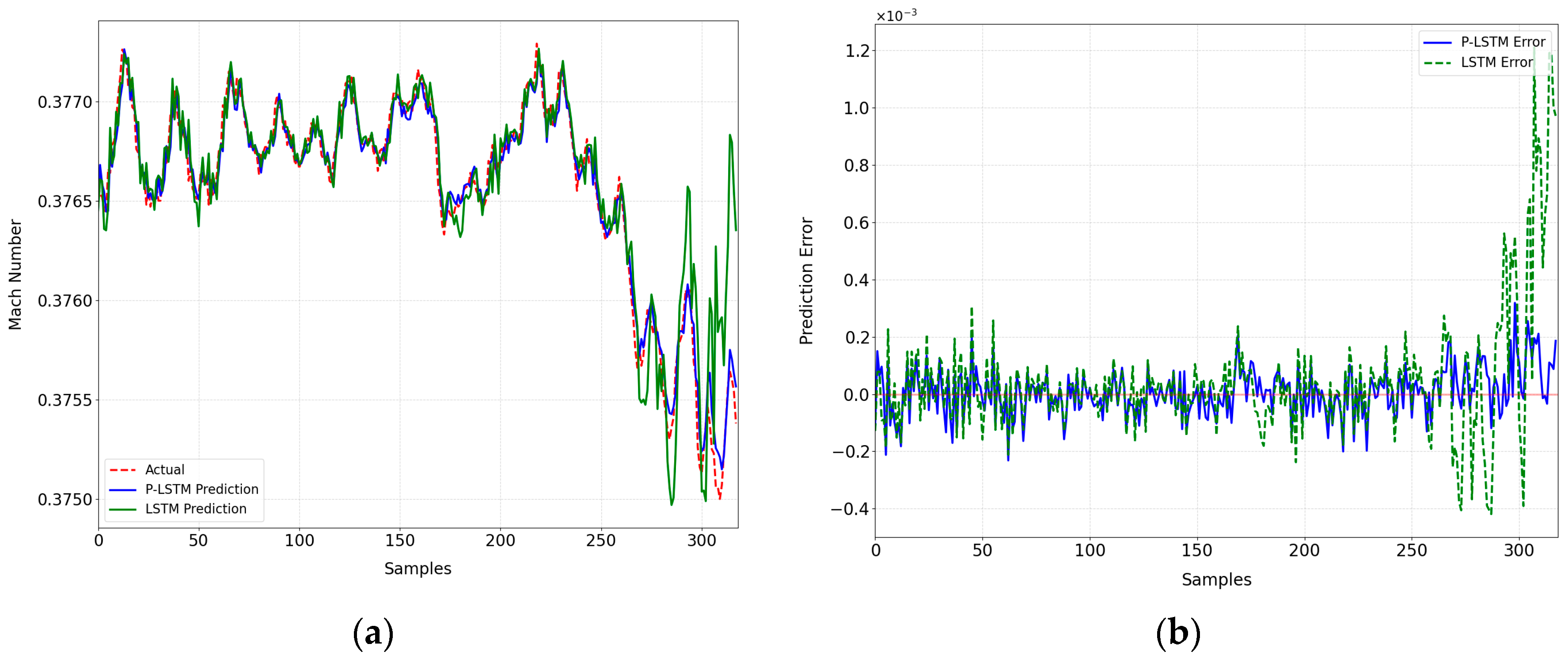
In the prediction model of P-LSTM, experimental validation is conducted using datasets under three typical operating conditions: 70% of the data is allocated to the training set, and the remaining 30% serves as an independent test set. Furthermore, to verify the prediction efficacy and physical constraint advantages of the model, comparative experiments are performed between P-LSTM and traditional LSTM methods. The dynamic prediction performance disparities of the two models in complex flow fields are quantitatively analyzed using three metrics: RMSE, MAE, and MD.

Figure 10, Figure 11, and Figure 12 respectively present the prediction results and error charts of the two Mach number models under working condition 1, working condition 2, and working condition 3. Based on the visual characterization of the prediction results and errors under three working conditions, the P-LSTM model shows higher accuracy in capturing the Mach number trend and closely matches the actual measurement data. In contrast, the traditional LSTM model’s prediction curves significantly deviate from the actual values, and dynamic feature extraction is limited. To systematically verify the superiority of the P-LSTM model, three model evaluation indexes were constructed and analyzed quantitatively under three typical working conditions: working conditions 1, 2, and 3. The specific evaluation results are shown in

Table 7. Comparison of evaluation indexes of two algorithms under three working conditions.

Working Condition	Algorithm	RMSE/10−5	MAE/10−5	MD/10−4
Working condition 1	LSTM	16.305	12.031	5.324
	P-LSTM	7.696	6.163	2.006
Working condition 2	LSTM	22.291	12.632	12.104
	P-LSTM	8.351	6.517	3.185
Working condition 3	LSTM	8.947	7.643	2.331
	P-LSTM	4.415	3.512	1.215

.

Figure 10. LSTM and P-LSTM prediction results under working condition 1: (a) Prediction curve, (b) Error curve.

Figure 10. LSTM and P-LSTM prediction results under working condition 1: (a) Prediction curve, (b) Error curve.

Figure 11. LSTM and P-LSTM prediction results under working condition 2: (a) Prediction curve, (b) Error curve.

Figure 11. LSTM and P-LSTM prediction results under working condition 2: (a) Prediction curve, (b) Error curve.

Figure 12. LSTM and P-LSTM prediction results under working condition 3: (a) Prediction curve, (b) Error curve.

Figure 12. LSTM and P-LSTM prediction results under working condition 3: (a) Prediction curve, (b) Error curve.

As illustrated in Table 7, the Mach number forecast model built on the P-LSTM framework displays outstanding accuracy across three standard operational scenarios. When stacked against the conventional LSTM approach, the P-LSTM model slashes the RMSE by a substantial 50.65% to 62.54%, cuts the MAE by 48.00% to 54.05%, and reduces the MD by as much as 47.88% to 73.68%. These figures clearly show that the P-LSTM does not just hit higher marks in prediction precision but also proves more reliable in estimating Mach numbers across various conditions. The results make it evident that the P-LSTM approach offers not only better accuracy but also more consistent performance with less error variation across different operating environments. Overall, the P-LSTM model put forward in this study significantly surpasses the traditional LSTM in forecasting Mach number with greater reliability.

4.3.2. 2.4 m CWT Experiments

In model migration, the accurate measurement of the similarity of working conditions is a key prerequisite. In this section, the similarity analysis of the three historical working conditions and the new working condition data is carried out firstly, so as to filter the suitable old working condition data for model migration, and the specific analysis results are shown in

Table 8. Similarity between the new working conditions and the three old ones.

	Old Working Condition 1	Old Working Condition 2	Old Working Condition 3
Similarity	0.6566	0.6565	0.8075

.

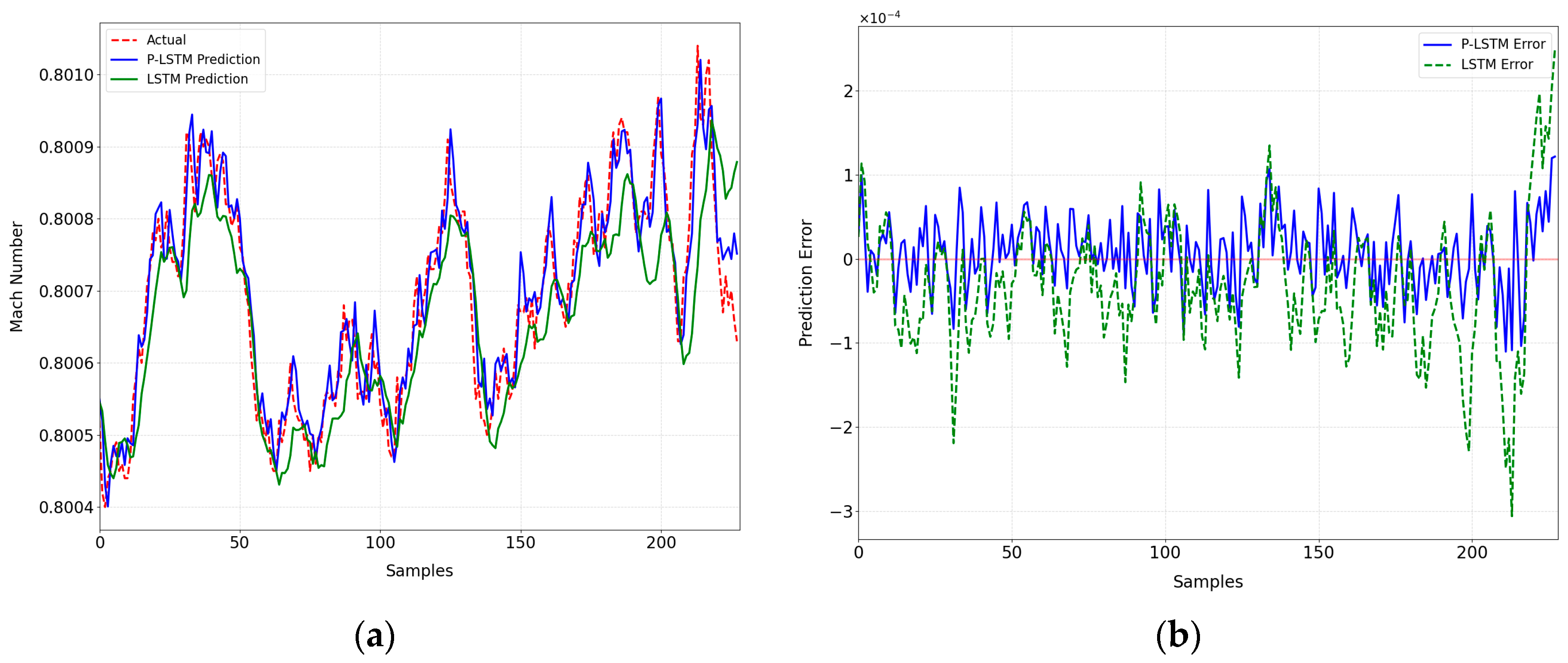
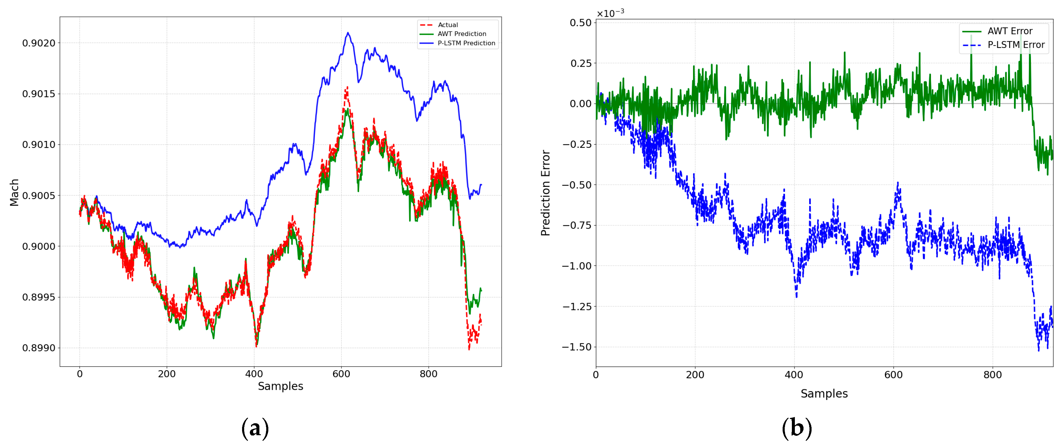
According to the results in Table 8, the old work condition 3 has the highest similarity with the new work condition, so the old work condition 3 is identified as the base data source for model migration. In the migration test design, the new condition data were split into two categories: one for training and the other for testing, in a 1:9 ratio. In order to verify the effectiveness of the migration strategy and highlight the advantages of the migration model, an independent P-LSTM model (non-migration model) is constructed based on the known data of 10% of the new conditions, and the actual gain of the migration strategy is quantitatively evaluated by comparing the prediction performance of this model with that of the AWTL model. Figure 13 compares prediction outcomes between the direct-trained and transfer models.

The analysis in

Table 9. Similarity analysis of new and old working conditions.

Algorithm	RMSE/10−4	MAE/10−4	MD/10−4
P-LSTM	7.752	7.114	15.26
AWTL	1.142	0.763	4.404

shows that the RMSE, MAE, and MD metrics of the AWTL model are significantly smaller than those of the non-migration model under the new operating conditions. Overall, the RMSE metrics of the AWTL model are reduced by 85.26%, MAE metrics by 95.12%, and MD metrics by 71.14% compared with the non-migration model. All the metrics of the AWTL model are better than the non-migration model, which proves the superiority of the proposed method in this paper. Therefore, the AWTL migration model, by fusing old working condition data with limited new working condition data, achieves efficient modeling of new conditions and avoids the large amount of manpower and material input required for traditional wind tunnel experiments.

5. Conclusions

To address the challenges of high-precision Mach number prediction and cross-domain modeling in wind tunnel tests, the P-LSTM model for Mach number prediction and the AWTL method for model migration are proposed in this study. A prediction system integrating physical interpretability and data-driven advantages is constructed. By embedding the isentropic flow equation from gas dynamics into the neural network loss function, the P-LSTM model effectively constrains the physically feasible domain of Mach number prediction, and reduces the RMSE by 50.65–62.54% compared with the traditional LSTM model in the 0.6 m CWT experiments, which verifies the capability of the physically data-driven modeling in capturing the time-sequence features of complex flow fields. Aiming at the scarcity of data in new wind tunnels, the AWTL method realizes efficient migration of wind tunnel models from 0.6 m to 2.4 m through cross-domain data calibration, dynamic optimization of sample weights in the source domain, and hybrid training in the target domain, which reduces the RMSE by 85.26% compared with non-migrated models in a 2.4 m wind tunnel scenario, and breaks through the limitations of the scaling effect and the scarcity of data. The research results provide a low-cost and high-precision modeling solution for wind tunnel tests, especially for the initial data-scarce scenarios of newly built wind tunnels, and have significant theoretical and application value for wind tunnel system optimization.

However, the P-LSTM and AWTL methods proposed in this paper are mainly targeted at continuous wind tunnel scenarios at this stage, and their extended applications in transient wind tunnels can be further explored in the future. It should be noted that this study did not consider the impact of model blockage effects on Mach number, which will be addressed as a key improvement direction in subsequent research.

References

1. Chen, C.; Klaus, T. Wind Tunnel Tests on the Unsteady Galloping of a Bridge Deck with Open Cross Section in Turbulent Flow. J. Wind. Eng. Ind. Aerodyn. 2023, 233, 105293. [Google Scholar] [CrossRef]
2. Huang, B.; Li, Z.; Gong, B.; Zhang, Z.; Shan, B.; Pu, O. Study on the Sandstorm Load of Low-rise Buildings Via Wind Tunnel Westing. J. Build. Eng. 2023, 65, 205821. [Google Scholar]
3. Esteban, A.; Elia, B.; Gisella, T. Evaluation of the Aerodynamic Effect of a Smooth Rounded Roof on Crosswind Stability of a Train by Wind Tunnel Tests. Appl. Sci. 2023, 13, 232. [Google Scholar]
4. Yang, X.; Wang, X.; Zhu, J.; Yan, W. Modelling, Analysis and Experimental Study of the Prop-rotor of Vertical/short-take-off and Landing Aircraft. Proc. Inst. Mech. Eng. Part G J. Aerosp. Eng. 2022, 236, 2851–2884. [Google Scholar] [CrossRef]
5. Zhang, L.; Ma, D.; Yang, M.; Yao, Y.; Yu, Y.; Yang, X. Experimental and Numerical Study on the Performance of Double Membrane Wing for Long-endurance Low-speed Aircraft. Appl. Sci. 2022, 12, 6765. [Google Scholar] [CrossRef]
6. Jarugumilli, T.; Benedict, M.; Chopra, I. Wind Tunnel Studies on a Micro Air Vehicle-scale Cycloidal Rotor. J. Am. Helicopter Soc. 2014, 59, 1–10. [Google Scholar] [CrossRef]
7. Li, J.; Wang, H.; Huang, H.L. Application of High-speed Wind Tunnel Control Based on PID Neural Network. Adv. Eng. Forum 2011, 2–3, 3–6. [Google Scholar] [CrossRef]
8. Andrei, N.C. Blowdown wind tunnel control using an adaptive fuzzy PI controller. INCAS Bull. 2013, 5, 89–98. [Google Scholar] [CrossRef]
9. Guo, J.; Zhang, R.; Cui, X.; Tianle, H.; Xin, H.; Zhao, L. Model Transfer and Fuzzy PID Control of Mach Number of Wind Tunnel Flow Field. In Proceedings of the 2020 Chinese Automation Congress (CAC), Shanghai, China, 6–8 November 2020; pp. 6923–6927. [Google Scholar]
10. Manitius, A. Feedback Controllers For a Wind Tunnel Model Involving a Delay: Analytical Design and Numerical Simulation. IEEE Trans. Autom. Control. 1984, 29, 1058–1068. [Google Scholar] [CrossRef]
11. Ouyang, J.; Liao, Y.-T.; Li, Y.; Wang, W.-H. Prediction of Transonic and Subsonic Wind Tunnel Aerodynamic Data by Neural Networks. J. Chin. Soc. Mech. Eng. 2022, 43, 509–520. [Google Scholar]
12. Wang, X.; Yuan, P.; Mao, Z. The Modified Feature Subsets Ensemble Applied for the Mach Number Prediction in Wind Tunnel. IEEE Trans. Aerosp. Electron. Syst. 2016, 52, 863–874. [Google Scholar] [CrossRef]
13. Chen, J. Improving performance of ensemble prediction models for Mach number in wind tunnels using metalearning. J. Aerosp. Eng. 2024, 37, 04024016. [Google Scholar] [CrossRef]
14. Salehi, H.; Burgueño, R. Emerging Rrtificial Intelligence Methods in Structural Engineering. Eng. Struct. 2018, 171, 170–189. [Google Scholar] [CrossRef]
15. Hochreiter, S.; Schmidhuber, J. Long Short-term Memory. Proc. Inst. Mech. Eng. Part G J. Aerosp. Eng. 1997, 9, 1735–1780. [Google Scholar] [CrossRef] [PubMed]
16. Zhang, R.; Liu, Y.; Sun, H. Physics-guided Convolutional Neural Network (PhyCNN) for Data-driven Seismic Response Modeling. Eng. Struct. 2020, 215, 110704. [Google Scholar] [CrossRef]
17. Guo, J.; Wang, W.; Guo, J.; Ariano, A.; Bosi, T.; Zhang, Y. An Instance-based Transfer Learning Model with Attention Mechanism for Freight Train Travel Time Prediction in the China–Europe Railway Express. Expert Syst. Appl. 2024, 251, 123989. [Google Scholar] [CrossRef]
18. Kang, S.; Xing, Y.; Wang, Y.; Wang, Q.; Xie, J. An Unsupervised Deep Model Transfer-based Method for Rolling Bearing Remaining Useful Life Prediction. Acta Autom. Sin. 2023, 49, 2627–2638. [Google Scholar]
19. Quionero, J.; Sugiyama, M.; Schwaighofer, A.; Lawrence, N.D. Dataset Shift in Machine Learning; MIT Press: Cambridge, MA, USA, 2009. [Google Scholar]
20. Li, L.; Wang, Z.; Chen, J.; Lu, F.; Huang, D.; Yang, H.; Li, Q. A Model Transfer Method Based on Transfer Component Analysis and Direct Correction. Spectrosc. Spectr. Anal. 2024, 44, 3399–3405. [Google Scholar]
21. Zhao, L.; Shao, Y.; Jia, W. NARX-Elman Based Mach Number Prediction and Model Migration of Wind Tunnel Conditions. Aerospace 2023, 10, 498. [Google Scholar] [CrossRef]
22. Yi, F.; Li, X.; Du, N.; Yu, W. An Iterative Learning-based Method for Wind Tunnel Mach Number Control. Control. Eng. 2020, 27, 109–113. [Google Scholar]
23. Olah, C. Understanding LSTM Networks, Colah’s Blog. 2016. Available online: https://colah.github.io/posts/2015-08-Understanding-LSTMs/ (accessed on 15 June 2025).
24. Zhang, R.; Liu, Y.; Sun, H. Physics-informed Multi-LSTM Networks for Metamodeling of Nonlinear Structures. Comput. Methods Appl. Mech. Eng. 2020, 369, 113226. [Google Scholar] [CrossRef]
25. Anderson, J. EBOOK: Fundamentals of Aerodynamics (SI Units); McGraw Hill: Columbus, OH, USA, 2011. [Google Scholar]
26. Wang, S.; Teng, Y.; Perdikaris, P. Understanding and Mitigating Gradient Flow Pathologies in Physics-informed Neural Networks. SIAM J. Sci. Comput. 2021, 43, A3055–A3081. [Google Scholar] [CrossRef]
27. Abbas, N.; Riaz, M.; Does, R.J.M.M. Enhancing the performance of EWMA charts. Qual. Reliab. Eng. Int. 2011, 27, 821–833. [Google Scholar] [CrossRef]
Figure 1. Schematic diagram of the 0.6 m continuous wind tunnel structure.
Aerospace 12 00701 g001
Figure 2. 2.4 m continuous wind tunnel.
Aerospace 12 00701 g002
Figure 4. Architecture of a deep LSTM network.
Aerospace 12 00701 g004
Figure 5. Schematic structure of a single LSTM cell.
Aerospace 12 00701 g005
Figure 6. Schematic architecture of the P-LSTM model.
Aerospace 12 00701 g006
Figure 7. MAE and RMSE for P-LSTM models with different time steps.
Aerospace 12 00701 g007
Figure 8. MAE and RMSE for P-LSTM models with different batch size.
Aerospace 12 00701 g008
Figure 9. MAE and RMSE for P-LSTM models with different neurons.
Aerospace 12 00701 g009
Figure 13. AWTL and P-LSTM prediction results under new working condition: (a) Prediction curve, (b) Error curve.
Aerospace 12 00701 g013