Article

A Multi-Mode Dynamic Fusion Mach Number Prediction Framework

College of Information Science and Engineering, Northeastern University, Shenyang 110819, China
*
Author to whom correspondence should be addressed.
Aerospace 2025, 12(7), 569; https://doi.org/10.3390/aerospace12070569
Submission received: 12 May 2025 / Revised: 18 June 2025 / Accepted: 21 June 2025 / Published: 23 June 2025
(This article belongs to the Special Issue New Results in Wind Tunnel Testing)

Abstract

The precise control of Mach numbers in supersonic and hypersonic compressor wind tunnel systems is a critical challenge in aerodynamic research. Although existing studies have improved prediction accuracy to some extent through machine learning methods, they generally neglect the multi-mode characteristics of complex wind tunnel systems, limiting the generalizability of the models. To address this issue, the present study proposes a multi-mode dynamic fusion Mach number prediction framework that integrates strategies of segmented modeling and cross-modal information fusion. First, single-mode segmented prediction models are constructed on the basis of Multi-output Support Vector Regression (MSVR), with hyperparameters optimized to capture the characteristics of individual modes. Second, the Partial Least Squares (PLS) method is employed to explore the correlations between historical and new modes, dynamically selecting the optimal prediction model and updating the historical mode repository. Experimental results demonstrate that the multi-mode dynamic fusion framework reduces the Root Mean Square Error (RMSE) by 70.57%, 56.4%, and 63.64% compared to Support Vector Regression (SVR), PLS, and Long Short-term Memory (LSTM) networks across six operating conditions. The framework proposed in this paper enhances Mach number prediction accuracy while improving model generalizability.

1. Introduction

Wind tunnel systems are the core infrastructure for aerodynamics research [1,2,3,4,5], offering experimental capabilities across subsonic [6], transonic, supersonic [7], and hypersonic regimes [8]. For example, in a low-speed wind tunnel, a static test of a conceptual advanced jet trainer was performed within the angle-of-attack range relevant to take-off and landing conditions [9]. At Iran’s National Low-Speed Wind Tunnel, static wind tunnel tests measured ground effect on the aerodynamic coefficients of a delta-wing aircraft during take-off and landing simulations [10]. At the INCAS trisonic wind tunnel, an experimental investigation determined the pitch damping coefficient and assessed the effects of Mach number, angle of attack, reduced frequency, center of rotation, and roll angle on pitch damping [11]. Colorado State University’s supersonic wind tunnel investigates supersonic combustion physics for future air-breathing hypersonic aircraft engines [12], while California Polytechnic State University’s supersonic wind tunnel studies the aerodynamics of bluff bodies undergoing dynamic orientation changes in supersonic flows, deepening the understanding of Mach effects under dynamic conditions [13].
Precise control of test conditions is fundamental for obtaining reliable wind tunnel data. Specifically, the accuracy, response speed, and stability of Mach number control within the test section flow field are key indicators for assessing wind tunnel system performance. Although often less critical in subsonic tunnels, precise Mach number control is paramount in supersonic and hypersonic compressor tunnels [14], as even minor velocity deviations can significantly alter aerodynamic and thermodynamic behavior. Studies [15,16,17] have indicated that the total pressure recovery coefficient decreases with increasing Mach numbers, while the total pressure distortion index approximately doubles. Furthermore, pressure-coefficient distributions are highly sensitive to the inflow Mach number: at subsonic speeds, these distributions remain relatively constant; however, at transonic and supersonic speeds, regions of positive pressure expand downstream while negative-pressure regions contract. However, the continuous advancement of wind tunnel systems has increased their complexity, introducing challenges such as non-linearities, time delays, strong coupling effects [18], and inherent uncertainties. Consequently, precise control of test section Mach numbers has become progressively more complex and technically demanding.
Data-driven approaches have become a research direction for precise Mach number prediction and control in these complex systems [19,20]. For instance, Wang and Mao [21] developed a Mach number prediction model based on an adaptive network-based fuzzy inference system to address computational burdens and accuracy degradation caused by excessive input variables. Yu et al. [22] recognized the dynamic variations of Mach numbers and established distinct prediction models using radial basis function neural networks and long short-term memory networks to handle steady-state and dynamic Mach number fluctuation processes, respectively. Chen [23] advanced ensemble modeling by proposing a meta-learning-based integrated fusion method to overcome accuracy limitations of traditional ensemble approaches in wind tunnel Mach number prediction.
These studies have effectively addressed the complex nonlinear relationships between Mach numbers and wind tunnel parameters, achieving notable prediction accuracy. However, existing models neglect the multi-mode operational characteristics inherent in wind tunnel systems. The multi-mode characteristics are manifested as significant variations in dynamic response properties under changing flow-field conditions, test types, and experimental requirements [24,25]. Different test modes correspond to specific aerodynamic parameter configurations (e.g., preset Mach numbers and rotational speeds), while individual test modes typically encompass multiple experimental batches. Taking fixed-Mach-number testing as an illustration, adjusting the angle of attack (AoA) from 0° to 1° and subsequently to 2° constitutes two distinct experimental batches. Such operational complexity poses substantial challenges to models’ cross-mode generalizability [26]. Consequently, there exists significant research value in effectively extracting critical inter-mode information features from wind tunnel systems and developing analytical models with enhanced cross-mode generalization abilities.
In industrial production systems, multi-mode problems have long been extensively studied as critical challenges [27]. Existing research primarily revolves around two methodological frameworks: (1) constructing hierarchical models that utilize shared modules to capture cross-mode commonalities while employing dedicated modules to characterize differentiated features across operational modes [28,29,30]; and (2) implementing targeted modeling strategies through operation-mode-based sub-model libraries [31,32,33] or adaptive updating mechanisms [34]. Wind tunnel systems exhibit multi-mode operational characteristics that bear significant parallels to complex industrial processes, particularly in managing systems with multiple operating regimes and discrete modes. The two domains face analogous challenges, including operational mode transitions, state monitoring, and system identification, while also sharing core technical requirements for robust control and precise dynamic modeling. Consequently, integrating these industrial modeling paradigms with wind tunnel aerodynamic phenomena, such as transonic flow transitions and Reynolds number dependencies, makes it possible to overcome the limitations of conventional single-point/single-condition modeling [35]. This synthesis presents novel solutions for predicting complex aerodynamic behaviors under variable test conditions and evolving flow regimes.
To address the specific challenges of wind tunnel testing and limitations in existing approaches, this study proposes the Multi-mode Dynamic Fusion Framework for Mach Number Prediction (MDF). This novel framework integrates segmented process modeling with multi-mode feature fusion, enabling more accurate and stable Mach number predictions. Furthermore, it ensures effective model adaptation through a selective update strategy, maintaining high prediction accuracy while preventing redundancy in the historical mode repository. Significantly, by analyzing regression coefficients between operational modes, the framework reveals dynamic response relationships across working modes.
The paper is organized as follows: Section 2 introduces the specific wind tunnel system studied in this paper. Section 3 presents the proposed framework, MDF. In Section 4, the model is validated through its application to Mach number prediction using real wind tunnel testing data, and comparative experiments are also conducted. The conclusions are summarized in Section 5.

2. Materials

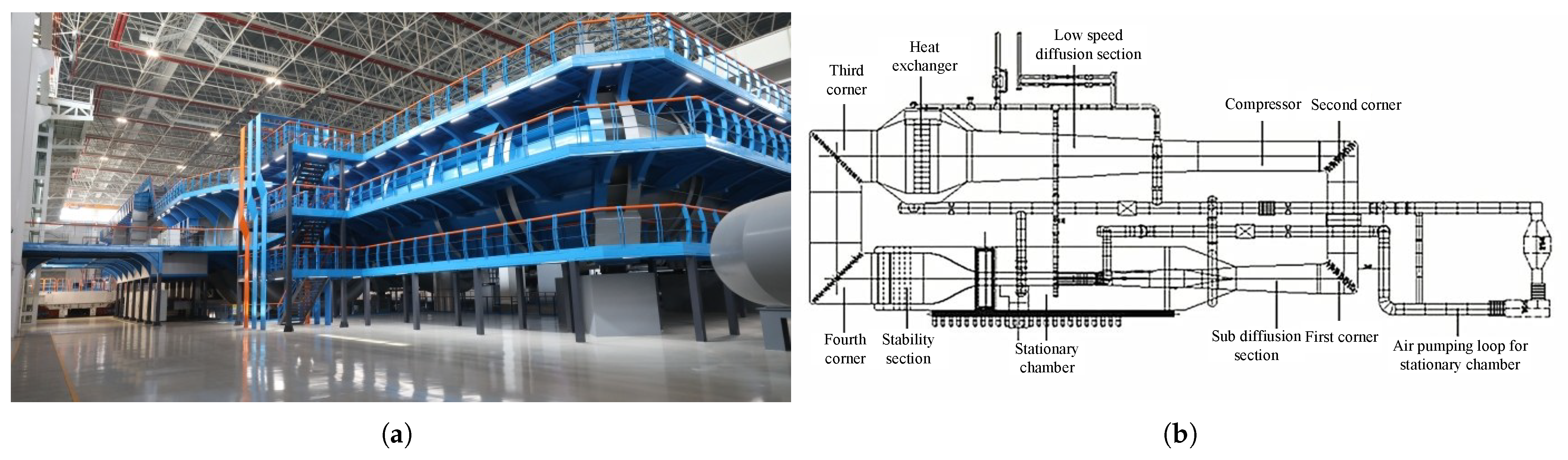
2.1. Continuous Transonic Wind Tunnel

The structural configuration and a full-view photograph of a 2.4 m continuous transonic wind tunnel are presented in Figure 1. This wind tunnel is a major large-scale facility in China, designed for aerodynamic testing and validation of aircraft configurations. Key specifications include a 2.4 m × 2.4 m test section, a Mach number range of 0.3–1.6, a total pressure range of 0.03–0.4 MPa, a total temperature range of 293–333 K, and a maximum Reynolds number of 1.3 × 10⁷.
The wind tunnel system is primarily composed of four corner sections, a heat exchanger, a compressor, and a test section. During operational initialization, the experimental procedure involves first adjusting the total pressure and controlling the compressor speed to achieve the preset Mach number, then initiating variable-AoA testing. The aircraft model’s orientation is modified according to predefined angular rates and angular ranges. However, this angular adjustment introduces significant disturbances to the flow field, causing Mach number deviations exceeding allowable control tolerances. Consequently, simultaneous adjustment of compressor speed is required to stabilize the Mach number within specified precision limits during AoA variations. Upon completion of data acquisition throughout this process, the AoA is reset to zero, facility shutdown procedures are executed, and the wind tunnel system is restored to its initial state for subsequent experimental preparations.

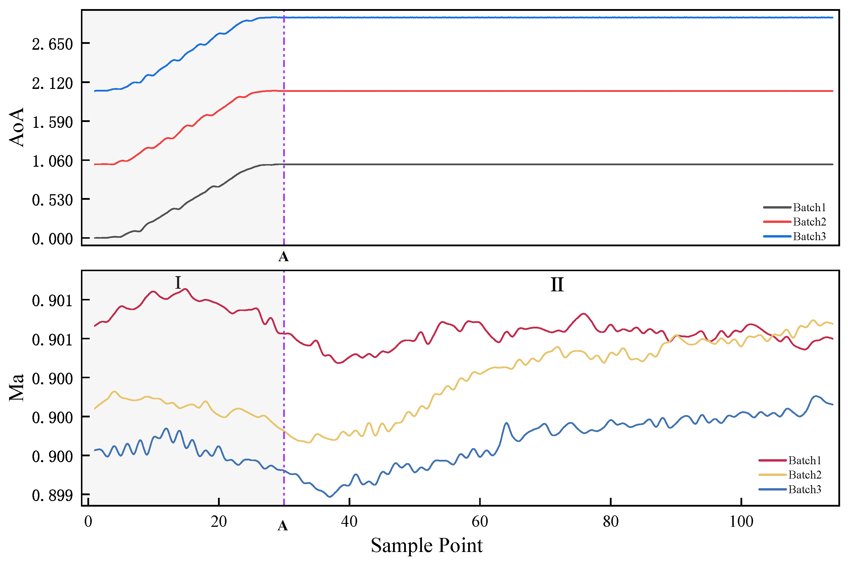
2.2. Mach Number and Its Effects

The Mach number is the ratio of an object’s velocity to the speed of sound and is a dimensionless quantity. In wind tunnel experiments, the Mach number of the test section is crucial, as this section carries the aircraft model, simulating the flight environment of the aircraft in the sky. Currently, there is no direct and precise instrument to measure the Mach number, and so it must be indirectly calculated by measuring the total pressure ( P o ) in the settling chamber and the static pressure ( P s ) in the test section. Additionally, the specific calculation methods vary for different speed ranges (subsonic, transonic, supersonic, and hypersonic). For an ideal gas with a specific heat ratio of 1.4, the flow from subsonic to supersonic speeds satisfies the following standard formula:
M a = 5 ( P o P s ) 2 7 1 .
Based on the above expression and the principles of error propagation, the theoretical accuracy [36] of the Mach number can be expressed as
Δ M a M a = 1 7 1 + 5 M a 2 Δ P o P o 2 + Δ P s P s 2 .
Owing to the relatively large absolute values of total pressure P o and static pressure P s , their relative measurement errors, Δ P o / P o and Δ P s / P s , are typically very small. Theoretically, the Mach number calculated from the corresponding formula can achieve extremely high accuracy. However, this is difficult to realize in practical engineering applications.
The subject of this study is a transonic wind tunnel, where engineering practice requires the Mach number control accuracy to satisfy | Δ M a | 0.001 in order to achieve effective control performance. Therefore, the Mach number prediction accuracy must reach the order of magnitude of 1 × 10⁻⁴.

3. Methodology

3.1. Multi-Mode Dynamic Fusion Framework for Wind Tunnel Mach Number Prediction

This study proposes MDF to address the multi-mode characteristics inherent in wind tunnel tests. The method initiates with phase partitioning of experimental data based on variations in the AoA. The dataset collected prior to phase partitioning within an experimental batch is defined as A = x j k 1 j N , 1 k M , where k denotes the sampling point index, N represents the number of variables, and M indicates the number of samples. After phase partitioning, the dataset is divided into C mutually exclusive subsets, denoted as S A C = S c ( a c , b c ) 1 c C , where a c denotes the starting time point of the cth subset, b c represents the ending time point of the cth subset, and the starting time point of each subset satisfies a c = b c 1 + 1 relative to its preceding subset.
Normalization is crucial in this framework, especially when dealing with extensive data splitting and reorganization. To ensure consistency and rationality in data preprocessing, normalization should be performed after all data splitting and reorganization operations are completed.
The data of each subset are normalized using the standardization method shown in Equation (3). Here, x j k c ˜ denotes the normalized value of x j k c , μ c is the mean of the cth subset, and σ c is the standard deviation of the cth subset.
x j k c ˜ = x j k c μ c σ c ( 1 j N , 1 k M ) . μ c = k = a c b c x j k c b c a c + 1 σ c = k = a c b c x j k c μ c 2 b c a c + 1
The preprocessed phase data S c ˜ ( a c , b c ) are utilized as input to establish MSVR-based sub-prediction models for distinct experimental phases. These sub-models are integrated to form single-mode prediction models. This process is iteratively executed across multiple modes to generate mode-specific prediction models. Representative modal models are then selected to construct a historical mode repository. Subsequently, PLS is employed to learn regression relationships between new modes and historical mode data, thereby establishing a multi-mode prediction model based on historical patterns.
The optimal predictive model was ultimately determined through systematic comparison of the two models’ performance metrics. This model was then applied as the Gaussian process’s prior mean function to quantify operational uncertainties and stochastic variability in real-world conditions, enhancing safety control under uncertainty.

3.2. Single-Mode Segmented Prediction Model for Mach Numbers

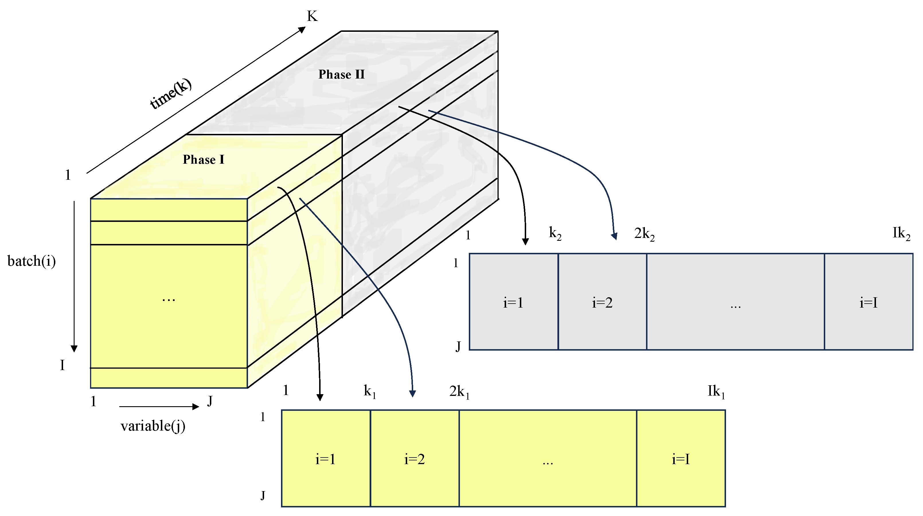
3.2.1. Wind Tunnel Test Phase Division

In wind tunnel tests, to simulate the changes in airflow direction experienced by an aircraft during actual operation, it is often necessary to adjust the aircraft’s angle after the Mach number reaches a preset stable point, i.e., to change the AoA. The variation in AoA significantly affects the Mach number within the wind tunnel system. As the AoA changes, the flow pattern of the air undergoes dramatic shifts, and these disturbances directly impact the flow state within the wind tunnel, making it difficult for the Mach number to remain stable within the desired accuracy range [37]. In such cases, to ensure the stability of the Mach number, it is necessary to adjust the compressor speed appropriately while changing the AoA so that the Mach number can stabilize within the desired accuracy range, thereby ensuring the accuracy and reliability of the experimental data.
Therefore, based on the variation in the AoA during the experiment, a complete test batch is divided into two stages. The specific division criteria are shown in Equation (4), where α target is the target AoA, α ( t ) represents the instantaneous AoA at time t, and ε is the allowable error threshold:
Δ α ( t ) = α ( t ) α target ε .
In wind tunnel tests, when the AoA starts to change and continues until it reaches and stabilizes at the preset target value, this process is defined as the ’transitional phase’. The period from when the AoA stabilizes at the target value until the next change in AoA occurs is defined as the ’steady-state phase’.
Figure 2 illustrates the Mach number variations during the transitional phase (Phase I) and steady-state phase (Phase II) for different test batches.
It can be observed that, as the AoA α changes, the Mach number undergoes significant fluctuations, deviating from the preset value. Additionally, due to the aerodynamic inertia of the wind tunnel system and the control loop delay, at sampling point A, although the AoA α has reached the target value and is stabilizing, the Mach number still fluctuates considerably over the next 5 to 6 sampling periods. Subsequently, under the control system’s influence, the fluctuations decrease, and the Mach number gradually returns to the preset value.

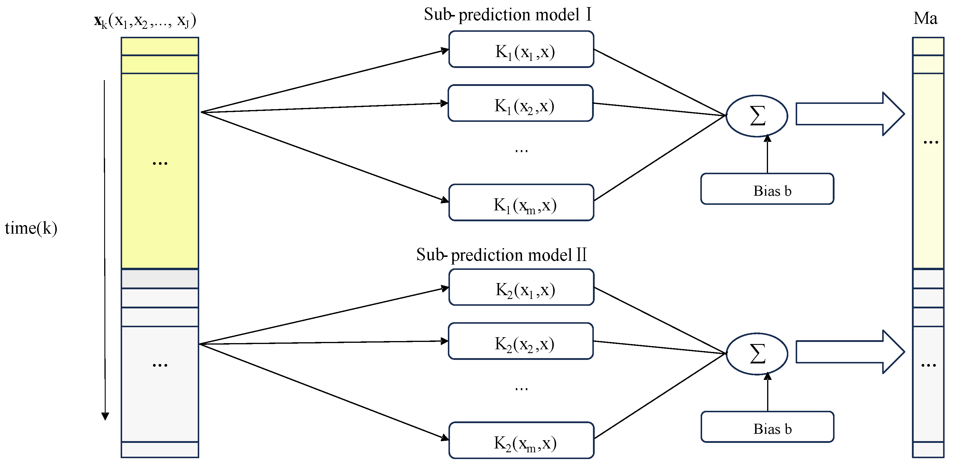
3.2.2. MSVR-Based Sub-Prediction Model

High-dimensional data variables are a characteristic of wind tunnel testing, as multiple test batches exist for experiments in the same mode. Denote the experimental data of I batches under a specific mode as G = A 1 , A 2 , , A I , which constitutes three-dimensional data. Direct modeling is infeasible, necessitating conversion into two-dimensional data prior to analysis. Formally, G is expressed as a third-order tensor X ( I × K × J ) [38], where I denotes the number of batch variables, K represents the number of sampling generations, and J corresponds to the number of selected variables.
The MSVR partitions the three-dimensional data matrix X ( I × K × J ) along the batch axis into data blocks across temporal and variable dimensions. These blocks are sequentially arranged into a new two-dimensional matrix X ( J × I K ) . Specifically, the original matrix X ( I × K × J ) is transformed into X ( J × I K ) .
Figure 3 demonstrates this process, where k 1 and k 2 represent sampling points in phase I and phase II, respectively. The partitioned matrices are strictly formatted as X ( J × I K 1 ) and X ( J × I K 2 ) . X ( J × I K 1 ) and X ( J × I K 2 ) are normalized via Equation (3) and subsequently utilized as input matrices for SVR training.
SVR, an adaptation of the Support Vector Machine (SVM) to regression problems, employs the hyperplane decision boundary from SVM as its regression model.
This method demonstrates superior performance in handling small-sample and high-dimensional data, exhibiting robust generalization capability for unknown samples. By leveraging kernel functions to map input data into high-dimensional feature spaces, SVR effectively captures complex nonlinear relationships. The fundamental mathematical formulation of SVR is expressed as [39].
For a given training dataset { ( x i , y i ) i = 1 , 2 , , m } , the regression model can be formulated as
f ( x ) = w T ϕ ( x ) + b ,
where w denotes the feature weight vector and b represents the bias term.
The optimization objective of SVR is formulated to identify the optimal hyperplane that simultaneously maximizes the margin and minimizes the total loss. To handle partially non-separable data points, slack variables ξ i and ξ ^ i are introduced, allowing certain samples to violate the margin constraints. The optimization problem of SVR is formulated as the following quadratic convex optimization problem:
min w , b 1 2 w 2 + C i = 1 m ( ξ i + ξ i ^ )      s . t . f ( x i ) y i ε + ξ i , y i f ( x i ) ε + ξ i ^ , ξ i 0 , ξ i ^ 0 , i = 1 , 2 , , m
where C > 0 is the penalty factor that balances the trade-off between model complexity (regularization term 1 2 w 2 ) and training errors (slack variables ξ i and ξ ^ i ).
A larger C prioritizes minimizing training errors, leading to higher model complexity and stronger fitting capability on the training data. However, excessively large C values may induce overfitting, where the model overemphasizes noisy training samples and loses generalizability. Conversely, overly small C values relax error constraints, potentially causing underfitting through oversimplified decision boundaries that fail to capture critical data trends. Therefore, it is critical to identify an optimal C to achieve a balance between generalization and empirical risk.
By introducing Lagrangian multipliers α i , α ^ i , μ i , and μ ^ i , Equation (5) is transformed into the corresponding Lagrangian function:
L w , b , ξ , ξ ^ , α , α ^ , μ , μ ^ = 1 2 w 2 + C i = 1 m ( ξ i + ξ ^ i ) i = 1 m ( μ i ξ i + μ ^ i ξ ^ i ) + i = 1 m α i f ( x i ) y i ε ξ i + i = 1 m α ^ i y i f ( x i ) ε ξ ^ i .
When we take the derivatives of the primal variables w , b , ξ i , and ξ ^ i and set them to zero, eliminating these primal variables leads to the following dual problem:
max α , α ^ i = 1 m y i ( α ^ i α i ) ε ( α ^ i + α i ) 1 2 i , j = 1 m ( α ^ i α i ) ( α ^ j α j ) K ( x i , x j ) s . t . i = 1 m ( α ^ i α i ) = 0 , 0 α i , α ^ i C .
After this problem is solved, the samples x i satisfying α i α ^ i 0 are called support vectors, and they determine the sparsity of the regression model. The final decision function of the model is expressed as
f ( x ) = i = 1 m ( α ^ i α i ) K ( x i , x ) + b .
In the formulation, the kernel function is defined as K ( x i , x ) = ϕ ( x i ) T ϕ ( x ) , and the bias term b is computed using support vectors lying precisely on the ε -tube boundary. Through the kernel trick, the model efficiently performs regression tasks in high-dimensional feature spaces. The kernel function must satisfy Mercer’s theorem [40] to guarantee its equivalence to an inner product in a Hilbert space. The choice of kernel function in SVR governs the geometric properties of the feature space, thereby influencing both model complexity and predictive accuracy. Consequently, the selection of the kernel function directly determines the model’s generalization performance.
Figure 4 illustrates the architecture of the MSVR-based sub-prediction model.
This study selects six process variables: the main compressor speed set point, the motor speed feedback, the total pressure in the test section ( P o ), the static pressure in the test section ( P c t ), the AoA, and the roll angle. These variables constitute the three-dimensional input data X ( I × K × J ) , where I denotes the number of batches, K represents the number of sampling points, and J indicates the number of process variables. The wind tunnel Mach number data serve as the output variable Y ( I × K ) . Both input and output variables are utilized as training data for the MSVR algorithm to construct an accurate prediction model.

3.2.3. Hyperparameter Tuning and Optimization

Given the significant impact of the penalty factor C and kernel function selection on the performance of the MSVR model, this study optimizes these two hyperparameters. Specifically, a Grid Search Cross-Validation method is employed to automatically identify the optimal kernel function and C value.
First, the hyperparameter search space is defined. The candidate values for C form an equidistant sequence, while the kernel function types include linear kernel (linear), radial basis function kernel (rbf), polynomial kernel (poly), and sigmoid kernel (sigmoid). Subsequently, 5-fold cross-validation is adopted to evaluate the generalizability of different parameter combinations. The grid search algorithm exhaustively traverses all possible parameter pairs and assesses their performance via cross-validation. Ultimately, the parameter configuration achieving the highest cross-validation accuracy is selected as the optimal model configuration.

3.3. Multi-Mode Prediction Model for Mach Number

Building upon the independent modeling of individual mode feature spaces (single-mode prediction models), this study further employs the PLS to explore relationships between new and historical modes, aiming to achieve synergistic modeling of cross-mode information complementarity. By establishing regression relationships between the outputs of individual single-mode prediction models and the Mach number of the new mode, a multi-mode prediction model is constructed. This model integrates both the new mode and historical modes from the historical mode repository. The PLS algorithm effectively extracts correlations between process inputs and outputs from stored historical data. The outputs of the new mode across all single-mode prediction models are rearranged into a k × v matrix X , while the Mach number values of the new mode form a k × 1 vector y .
By applying the PLS algorithm, the regression relationship between the new and historical modes can be formulated as follows:
X = T P + E ,
y = U q + f ,
where T R k × s and U R k × s are score matrices, and P R v × s and q R s × 1 are loading matrices, E R k × v and f R k × 1 are residual matrices.
U = T B + H ,
where B R s × s is the diagonal association matrix between latent variables, while H R k × s is the latent variable residual matrix. Consequently, the regression formulation can be derived as follows:
y ^ = X W ( P W ) 1 B q .
If we let β = W ( P W ) 1 B q , then, through substitution and simplification, we can obtain
y ^ = X β ,
where β R v × 1 is the regression coefficient. Specifically, β captures the extent and direction of the influence of each historical mode on the new mode. In the regression model, each component of β corresponds to the contribution of a specific historical mode, allowing us to quantify the impact of different historical modes on the prediction of the new mode, thereby enhancing the prediction accuracy and stability of the multi-mode wind tunnel system.

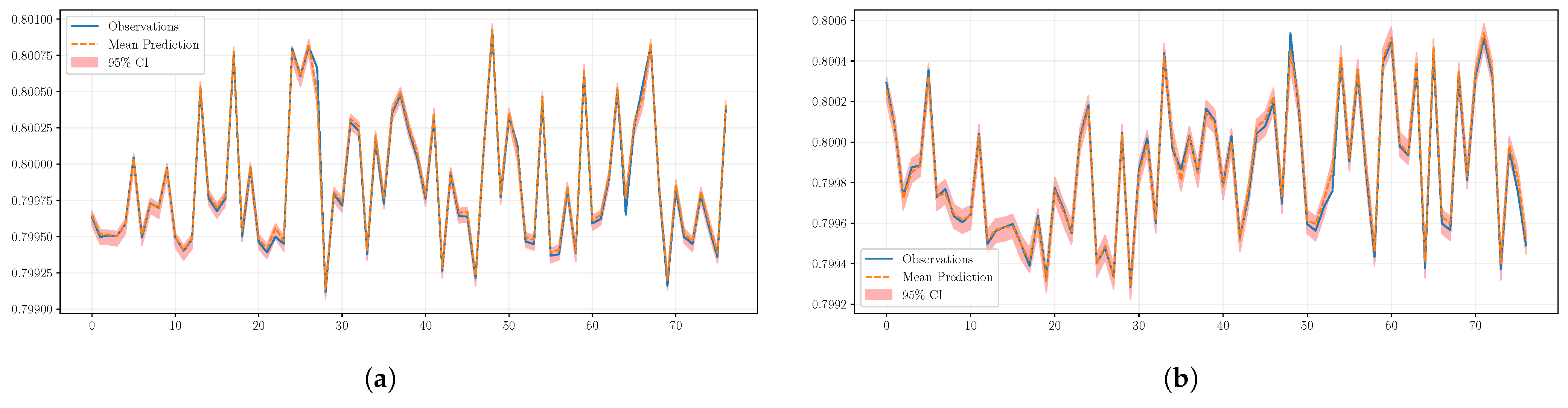
3.4. Uncertainty Quantification Framework

To address epistemic and aleatoric uncertainties, a Gaussian process postprocessor is employed. The Gaussian process learns the residual distribution between our base model predictions and experimental data, providing a standard deviation σ for each prediction. The final output becomes y ^ ± 1.96 σ (95% confidence interval). Considering the uncertainties caused by turbulent fluctuations in the wind tunnel system and noise in the data acquisition system, this paper employs a covariance function combining a radial basis function with a white noise kernel:
K x i , x j = exp x i x j 2 2 2 + σ n 2 δ i j .
For the test sample point x , the posterior probability follows a Gaussian distribution:
p y x , D = N μ , σ 2 ,
where
μ = k T K + σ n 2 I 1 y
σ 2 = k x i , x i k T K + σ n 2 I 1 k

3.5. Model Comparison and Selection with Historical Mode Repository Update

Given the uncertainty regarding the effectiveness of historical mode data for new data prediction, this study trains both single-mode and multi-mode prediction models separately on new data. Subsequently, the performance of these two models is evaluated and compared to determine whether updates to the historical mode repository are required. The specific workflow is illustrated in Figure 5. It is crucial to emphasize that the model selection in this section operates at the level of individual batches. In other words, even for the same mode, its predictive performance may vary across different batches due to persistent differences in statistical properties between batches. Therefore, it is necessary to select distinct prediction models for different batches.
For a normalized training set X t r a i n ( I × J × K ) and its corresponding actual Mach number tensor Y t r a i n ( I × K ) , both single-mode and multi-mode prediction models are trained using these datasets. The normalized test set X t e s t ( I × J × K ) is then fed into these two models to generate respective predictions: Y s ( I × K ) (single-mode) and Y m ( I × K ) (multi-mode). Following the methodology described in Section 3.2, each Mach number matrix Y ( I × K ) can be decomposed along the batch direction into I time-series vectors:
Y ( I × K ) = y 1 y 2 y I .
Subsequently, the evaluation computes the RMSE on the test set between the single-mode predictions y s i , multi-mode predictions y m i , and actual Mach values y t e s t i (from Y t e s t ). The single-mode prediction model’s RMSE is defined as
RMSE s i = 1 K k = 1 K y s , k i y test , k i 2 ,
and the multi-mode prediction model’s RMSE is defined as
RMSE m i = 1 K k = 1 K y m , k i y test , k i 2 .
The predictive performance of the two models is evaluated by comparing RMSE s i and RMSE m i . If the two prediction models satisfy
| RMSE s i RMSE m i | < ε ( ε = 10 5 ) ,
they are considered to have equivalent predictive efficacy. In such cases, the multi-mode prediction model with stronger generalizability is prioritized, under the underlying assumption that the feature space of the historical mode library adequately covers the distribution characteristics of the current test samples.
When there exists a significant performance disparity between the two prediction models,
| RMSE s i RMSE m i | ε ,
two scenarios emerge:
  • RMSE s i < RMSE m i :
    The single-mode predictor demonstrates superior performance, indicating that the test data contain novel features not covered by the historical mode repository. In this scenario, the single-mode model is selected as the final predictor, and the current sample’s feature vector X t e s t i and corresponding Mach number vector y t e s t i are incorporated into the historical mode repository.
  • RMSE s i > RMSE m i :
    The multi-mode predictor achieves better performance by leveraging historical mode information, suggesting that the historical mode repository sufficiently characterizes current operational conditions. In this case, the multi-mode model is chosen as the final predictor, and no repository update is performed to mitigate overfitting risks.

3.6. Offline Training and Online Prediction

During the offline phase, MSVR is employed to construct multiple sub-models based on different input features, with each sub-model trained using typical operating condition samples from the historical mode repository. The adopted dataset is relatively small, which, on one hand, ensures manageable computational costs during training and, on the other hand, guarantees that the training duration remains within an acceptable range. As offline training is temporally independent of the real-time control process, the relatively high computational overhead during training does not compromise the real-time performance of the wind tunnel control loop. In experimental execution, all sub-models complete training during the offline phase, ensuring the trained models can be directly utilized for Mach number prediction in the online phase without requiring retraining.
After offline training is completed, the sub-models are not frequently updated. Updates are only triggered when new operating condition types are identified or a declining trend in model prediction performance is detected. This initiates the update mechanism, which refreshes the historical mode repository library and trains new sub-models. This update strategy effectively reduces computational overhead for model maintenance, avoiding unnecessary repeated training and redundancy in the historical mode repository. When the environment and system states remain stable, the parameters of the sub-models are preserved unchanged, significantly reducing the computational resources and time required for training.
The offline phase of training involves only historical data and small-scale samples, thus ensuring computational costs remain highly manageable. The training process can be fully completed offline with sufficient computational resources, guaranteeing the validity and completeness of the models. Meanwhile, based on this offline design, the online phase requires only model inference and dynamic model comparison, eliminating the need for online training, which meets the response requirements of real-time wind tunnel control. Theoretically, the computational burden introduced by the designed multiple sub-models and dynamic comparison mechanisms during the offline phase remains acceptable and does not impose a bottleneck in practical applications.

4. Illustration and Discussion

As described in this section, twenty-one distinct operating conditions were analyzed and tested with detailed data presented in Table 1.
All data were collected from the wind tunnel test facility described in Section 2, with no denoising preprocessing applied. The selection of operating conditions was designed to ensure experimental diversity and representativeness, covering system performance across varied operational scenarios. These conditions were categorized into four operational modes, differentiated by key control parameters such as preset Mach number, preset main compressor speed, and rate of AoA variation.

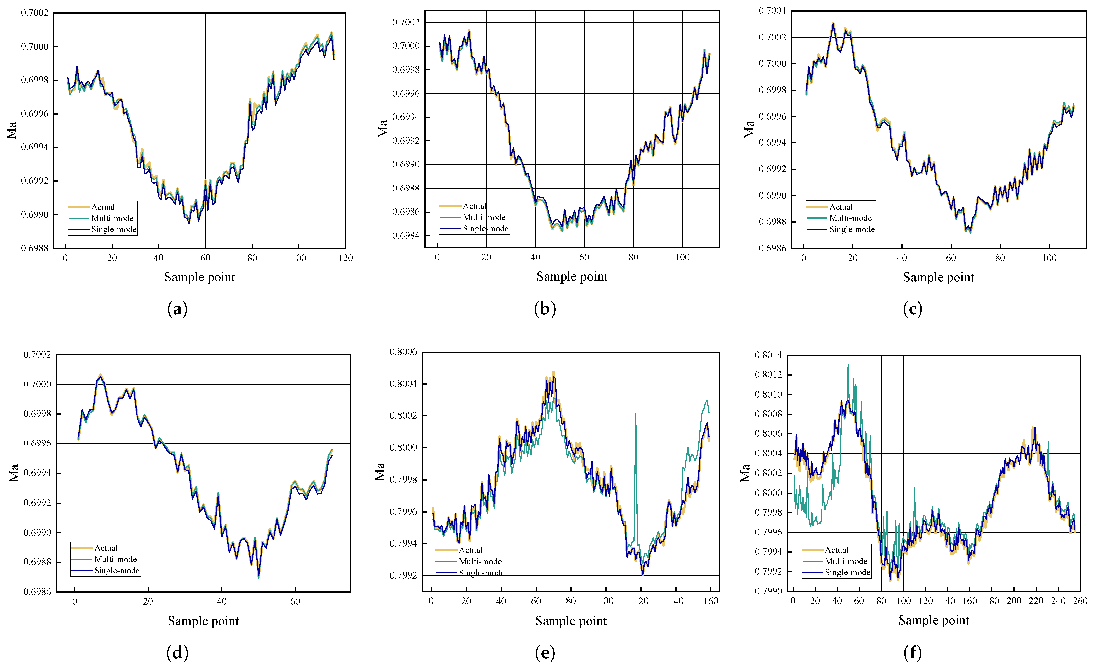
4.1. Design of Prediction Experiment and Analysis of Results

Data from Modes 2 and 4 were selected to construct a historical mode repository. A multi-mode prediction model was trained using this repository to predict the Mach numbers in Modes 1 and 3.
Individual single-mode prediction models were developed for each operational mode dataset. The hyperparameters of sub-predictors at each stage were optimized through fivefold cross-validation combined with grid search. The optimized hyperparameters and corresponding model R 2 values are listed in Table 2. Notably, the full dataset was employed for training models within the historical mode repository to maximize the utilization of historical data. For the prediction-targeted modes, a 7:3 split between training and test sets was implemented to prevent model overfitting and improve evaluation effectiveness.
Higher R 2 values are consistently observed in steady-state phases compared to transitional phases. This demonstrates superior model fitting and predictive capability for process variables during steady states, where smaller data variations and system stability prevail. This discrepancy primarily arises from the rapid parameter variations in transitional phases, which result in significantly fewer available samples than steady-state phases.
The multi-mode prediction model also adopted a 7:3 training–test split ratio. Comparative analysis between single-mode and multi-mode prediction models was performed for six operating conditions in Modes 1 and 3. As illustrated in Figure 6, actual Mach number curves, single-mode predictions, and multi-mode predictions are visually compared for these six conditions.
Comparable predictive performance is observed between the two models for the four operating conditions in Mode 1, both effectively capturing Mach number trends and variations. The multi-mode model demonstrates superior performance under scenarios with significant Mach number fluctuations, achieving more accurate tracking and stable predictions.
In contrast, for the two operating conditions in Mode 3, the multi-mode model underperforms despite the MSVR-based single-mode model maintaining satisfactory accuracy. In condition 12, while the multi-mode model captures the overall trend, significant deviations between predicted and actual Mach number curves are observed, with severe outliers degrading prediction precision. Similarly, condition 13 exhibits large deviations in the prediction curve’s initial segment and erroneous spikes at multiple time points.
The RMSE values of both models across operating conditions are compared in the Table 3. This comparison will determine the final predictive model.
Comparable RMSE values between the two prediction models are observed for Mode 1, satisfying the criteria defined in Equation (23). Thus, no update to the historical mode repository is required, and the multi-mode prediction model is selected as the final model. For Mode 3, the single-mode prediction model is chosen because RMSE s i < RMSE m i , with the data from Mode 3 incorporated into the historical mode repository to acquire new statistical features.
Experimental results indicate that for the new Mode 1, despite differences from historical modes, sufficient correlations exist to enable effective information extraction from the historical mode repository by the multi-mode model, ensuring successful predictions. In contrast, Mode 3 exhibits significant deviations from historical modes, as evidenced by its larger AoA step size and intense variation magnitude in Table 1. These discrepancies prevent the multi-mode model from adequately adapting to this new operational mode using existing historical data. The absence of statistical features related to Mode 3 in the historical mode repository leads to scale mismatch in the multi-mode model during processing, thereby degrading prediction accuracy.
After training with the new mode data, the MSVR-based single-mode prediction model demonstrates stable and satisfactory performance across all operating conditions. Notably, despite lacking dedicated training for new modes, the multi-mode model retains reasonable predictive capability, highlighting its adaptability and strong generalization. For Mode 1, which resembles historical modes, the multi-mode model is comparable in accuracy to the trained single-mode model, confirming its reliability in handling known or similar operational scenarios.
Figure 7 presents the Gaussian process test results after MDF prediction, demonstrating effective characterization of flow velocity uncertainties in the wind tunnel system. The majority of observed data points are contained within the 95% confidence interval (red band), confirming calibration reliability under dynamic flow conditions. If the confidence interval expands significantly, it indicates a potential system anomaly, and a risk alert should be issued promptly.
Table 4 presents the regression coefficients of test operating conditions on historical modes in the multi-mode prediction model.
From a physical perspective, a large coefficient indicates that the predictions of the corresponding sub-model align closely with the actual flow response in the current regime, while a coefficient near zero implies the sub-model contributes minimal new information. Sub-models whose physical characteristics extensively overlap with the current Mach regime receive higher weights, whereas those trained under significantly different conditions are assigned lower weights. Thus, the PLS regression process automatically selects and scales sub-models based on their relevance, effectively transferring physically meaningful information into the multi-mode prediction model.
As expected, for operating conditions 12 and 13, which deviate substantially from the historical mode repository, the weights assigned to the sub-models are notably low, further validating the previous explanation.

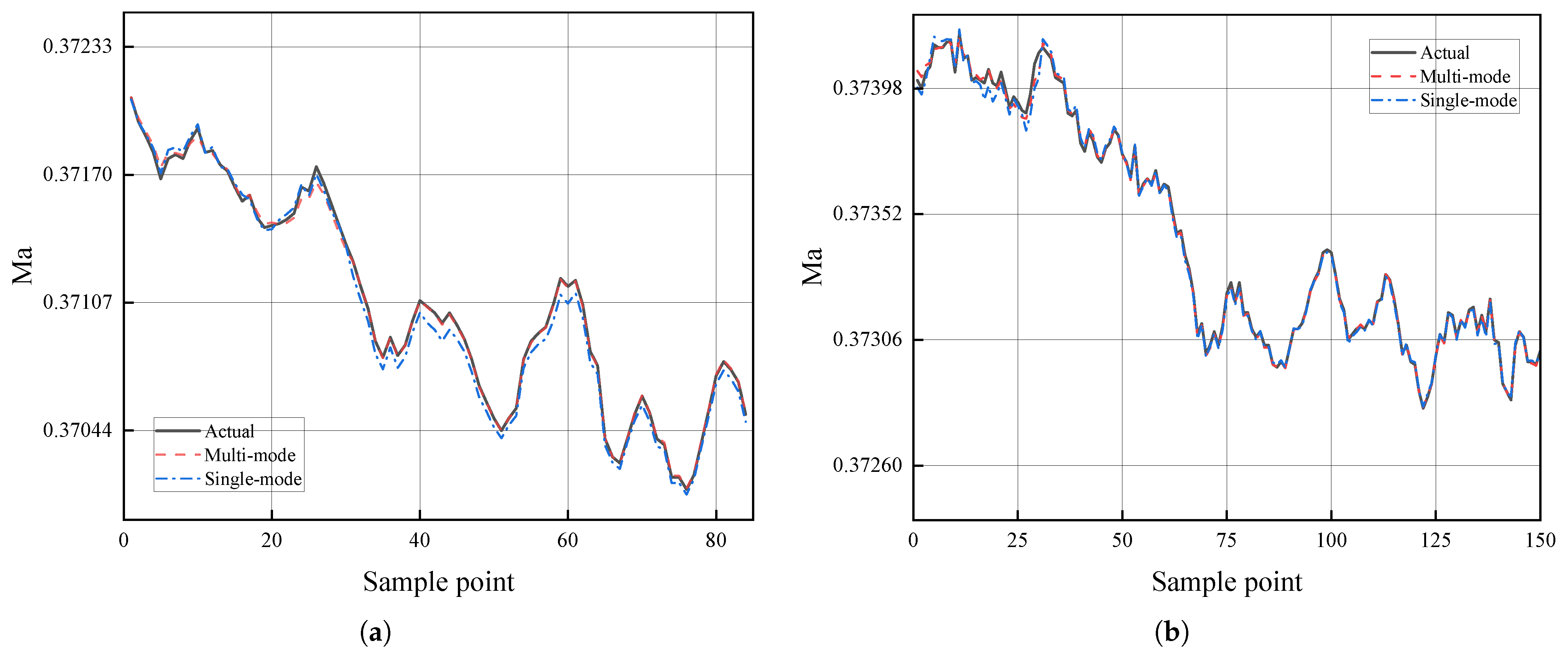
4.2. Mach Number Prediction for 0.6 m Wind Tunnel

To validate the applicability of the proposed model in other wind tunnels, an offline model was established using the typical operating modes of a 0.6 m wind tunnel. Mach number predictions were conducted for five operating conditions, with the corresponding RMSE values presented in Table 5.
Figure 8 illustrates a performance comparison between single-mode and multi-mode predictive models under two operating conditions within the same working mode.
The experimental results indicate that the multi-mode model demonstrates superior prediction performance compared to the single-mode model. The reasons are as follows: the limited data volume of single-operation conditions collected in the 0.6 m wind tunnel results in unsatisfactory prediction performance of the single-mode model, whereas the multi-mode model, by leveraging similarity information from historical mode repository, not only maintains good prediction performance but also ensures that all prediction outcomes meet the Mach number accuracy requirements.

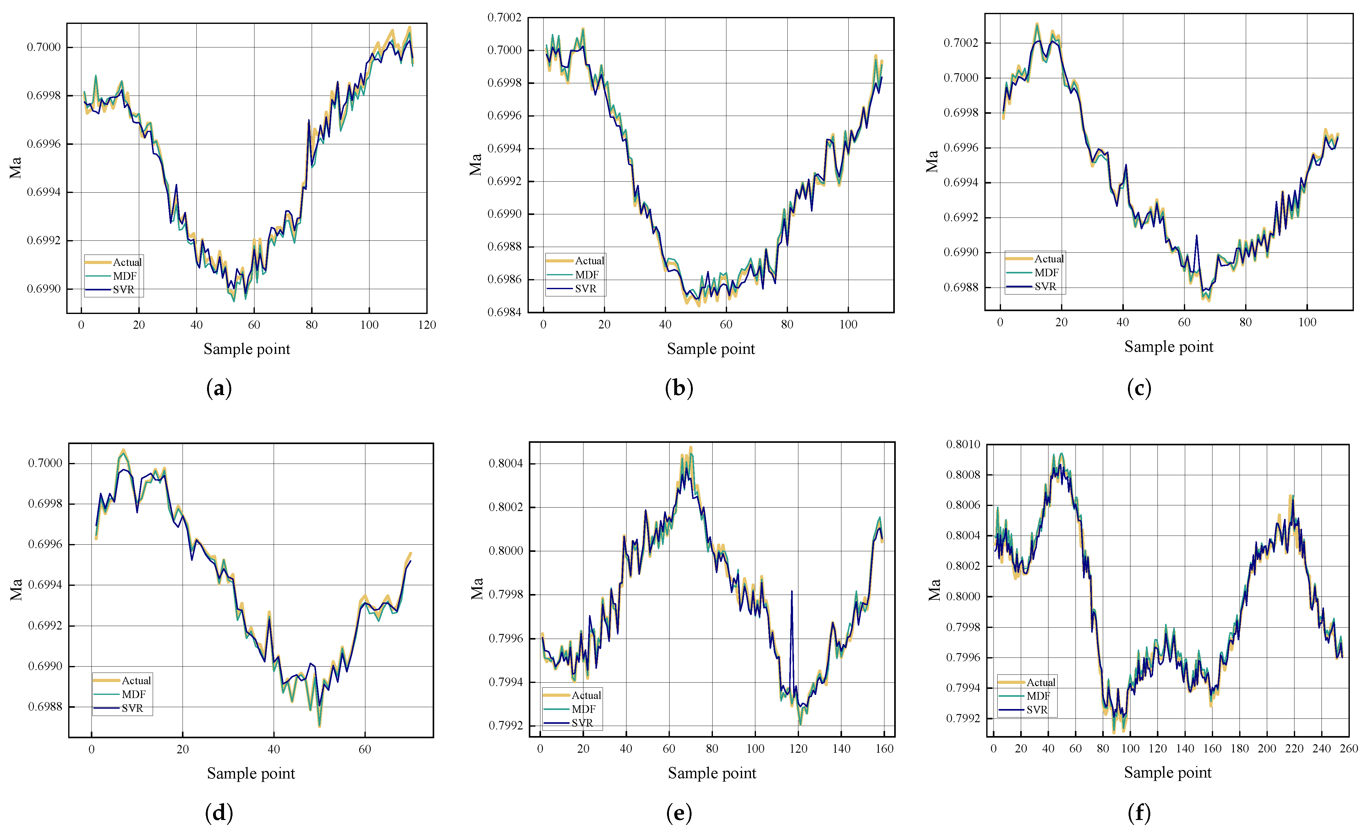
4.3. Comparison with Existing Methods

Comparative experiments are conducted on six representative operating conditions (conditions 1–4 and 12–13), including Mode 1 (closely aligned with the historical mode repository) and Mode 3 (exhibiting significant deviations from historical modes). A comparative analysis is conducted between the proposed method (MDF) and baseline methods, including conventional approaches (SVR, PLS) and deep learning models (LSTM), to assess performance differences.
The proposed method, MDF, is developed based on these two classical algorithms (SVR and PLS), incorporating a multi-mode dynamic fusion framework to simultaneously handle strong linear relationships and potential nonlinear interactions among variables in wind tunnel systems. By dynamically fusing information from different modes, MDF adaptively adjusts regression coefficients across modes, enabling precise capture of system dynamic patterns under both complex operating conditions and novel scenarios.
A comparative analysis of predictive performance among MDF, PLS, and SVR for Mach numbers in Modes 1 and 3 is systematically presented in Figure 9 and Figure 10, validating the effectiveness of integrating the two machine learning algorithms (PLS and SVR) into the MDF framework. A comparative evaluation of prediction accuracy across four algorithms is systematically presented in Figure 11.
The RMSE values of the four algorithms across all test operating conditions are summarized in Table 6.
Experimental results demonstrate that MDF maintains superior prediction accuracy across all test operating conditions, achieving average reductions in RMSE of 70.57% compared to conventional SVR, 56.4% versus PLS, and 63.64% against LSTM. This significant performance improvement indicates the enhanced prediction accuracy and stability of MDF when handling complex and dynamically varying operating conditions.
LSTM demonstrates intermediate performance across most test conditions. In condition 1, LSTM (3.846 × 10⁻⁵) outperforms PLS (5.974 × 10−5) by 35.6% and approaches SVR’s result (3.966 × 10⁻⁵), with only a 3.2% difference. However, its performance degrades notably in conditions 3 and 4, where its RMSE (5.102 × 10⁻⁵ and 5.038 × 10⁻⁵) exceeds those of all other models. This variability suggests LSTM’s sensitivity to specific operating regimes despite its theoretical capacity for temporal modeling. Crucially, MDF maintains consistent superiority over LSTM in all test conditions, with performance advantages ranging from 36.8% in condition 1 to 84.7% in condition 4. This demonstrates that while deep learning approaches like LSTM offer theoretical advantages for sequential data, their practical effectiveness in this application is constrained by operational complexities.

5. Conclusions

For a 2.4 m continuous wind tunnel, a novel Mach number prediction framework termed MDF is proposed. By integrating a single-mode segmented prediction model with multi-mode feature fusion, the proposed framework significantly enhances prediction accuracy and model generalization capability. The framework’s universality is further validated using experimental data from a 0.6 m wind tunnel, demonstrating that it meets the engineering requirements for Mach number prediction accuracy. Compared to traditional machine learning methods (SVR and PLS) and LSTM, the MDF demonstrates superior performance and stability. This dynamic fusion framework notably improves tracking capability for Mach number fluctuations, particularly in test environments characterized by high Mach number variability. Furthermore, this study emphasizes the importance of selectively updating the historical mode repository to adapt to new operational conditions. This strategy ensures effective model adaptation while maintaining high prediction accuracy and preventing repository redundancy. MDF delivers a high-precision, highly robust prediction tool for Mach number control in complex wind tunnel systems. By leveraging regression coefficients between operational modes, it provides useful insights into intricate system behaviors.
However, this work primarily focuses on the prediction framework itself. Future research should investigate Mach number control strategies integrated with the prediction model to enhance the practical utility of MDF.

Author Contributions

Conceptualization, L.Z.; methodology, L.Z. and W.L.; software, W.L.; validation, W.L. and W.X.; formal analysis, W.L.; investigation, L.Z.; resources, L.Z.; data curation, L.Z.; writing—original draft preparation, W.L. and W.X.; writing—review and editing, L.Z.; visualization, W.L. and W.X.; supervision, L.Z.; project administration, L.Z.; funding acquisition, L.Z. All authors have read and agreed to the published version of the manuscript.

Funding

This research was funded by the National Natural Science Foundation of China (No. 61503069) and the Fundamental Research Funds for the Central Universities (N2404010).

Data Availability Statement

The raw data supporting the conclusions of this article will be made available by the authors on request.

Acknowledgments

All data were provided by Aviation Technology Key Laboratory of Aerodynamics Research at High Speeds and High Reynolds Numbers, Shenyang 110819, China.

Conflicts of Interest

The authors declare no conflicts of interest.

References

  1. Zhao, Z.; Zhao, C.; Pei, Z.; Chen, W. Design and Implementation of a Low-Speed Wind Tunnel System. In Proceedings of the 2021 IEEE 16th Conference on Industrial Electronics and Applications (ICIEA), Chengdu, China, 1–4 August 2021; pp. 273–278. [Google Scholar]
  2. Tan, H.; Wang, J.; Bu, C.; Mu, W.; Shen, Y.; Chen, H. Development of wind tunnel dynamic test system for coupled motion with multi-degrees of freedom. In Proceedings of the CSAA/IET International Conference on Aircraft Utility Systems (AUS 2022), Nanching, China, 17–20 August 2022; Volume 2022, pp. 488–495. [Google Scholar]
  3. Mo, Z.; Fu, H.Z.; Ho, Y.S. Global development and trend of wind tunnel research from 1991 to 2014: A bibliometric analysis. Environ. Sci. Pollut. Res. 2018, 25, 30257–30270. [Google Scholar] [CrossRef] [PubMed]
  4. He, S.; Guo, S.; Liu, Y.; Luo, W. Passive gust alleviation of a flying-wing aircraft by analysis and wind-tunnel test of a scaled model in dynamic similarity. Aerosp. Sci. Technol. 2021, 113, 106689. [Google Scholar] [CrossRef]
  5. Aleisa, H.; Kontis, K.; Nikbay, M. Low Observable Uncrewed Aerial Vehicle Wind Tunnel Model Design, Manufacturing, and Aerodynamic Characterization. Aerospace 2024, 11, 216. [Google Scholar] [CrossRef]
  6. Abbaspour, M.; Shojaee, M. Innovative approach to design a new national low speed wind tunnel. Int. J. Environ. Sci. Technol. 2009, 6, 23–34. [Google Scholar] [CrossRef]
  7. Yu, K.; Xu, J.; Liu, S.; Zhang, X. Starting characteristics and phenomenon of a supersonic wind tunnel coupled with inlet model. Aerosp. Sci. Technol. 2018, 77, 626–637. [Google Scholar] [CrossRef]
  8. Jiang, Z.; Hu, Z.; Wang, Y.; Han, G. Advances in critical technologies for hypersonic and high-enthalpy wind tunnel. Chin. J. Aeronaut. 2020, 33, 3027–3038. [Google Scholar] [CrossRef]
  9. Taleghani, A.S.; Ghajar, A.; Masdari, M. Experimental Study of Ground Effect on Horizontal Tail Effectiveness of a Conceptual Advanced Jet Trainer. J. Aerosp. Eng. 2020, 33, 05020001. [Google Scholar] [CrossRef]
  10. Shams Taleghani, A.; Ghajar, A. Aerodynamic characteristics of a delta wing aircraft under ground effect. Front. Mech. Eng. 2024, 10, 1355711. [Google Scholar] [CrossRef]
  11. Bunescu, I.; Stoican, M.G.; Hothazie, M.V. Experimental Determination of Pitch Damping Coefficient Using Free Oscillation Method. Aerospace 2024, 11, 579. [Google Scholar] [CrossRef]
  12. Teeter, S.; Plese, K.; Zulch, R.; Haid, C.; Windom, B.; Yalin, A.P.; Dumitrache, C. Development of a Supersonic Wind Tunnel Facility for Scramjet Testing at Colorado State University. In Proceedings of the AIAA SciTech 2024 Forum, Orlando, FL, USA, 8–12 January 2024. [Google Scholar]
  13. Sanai, S.; Hiremath, N. Implementation of Rotating Test Stand for Supersonic Wind Tunnel. In Proceedings of the 2024 Regional Student Conferences, Santa Clara, CA, USA, 1 January 2024. [Google Scholar]
  14. Yu, K.; Xu, J.; Li, R.; Liu, S.; Zhang, X. Experimental exploration of inlet start process in continuously variable Mach number wind tunnel. Aerosp. Sci. Technol. 2018, 79, 75–84. [Google Scholar] [CrossRef]
  15. Damljanović, D.; Vuković, D.; Ocokoljić, G.; Rašuo, B. New Transonic Tests of HB-2 Hypersonic Standard Models in the VTI T-38 Trisonic Wind Tunnel. Aerospace 2025, 12, 131. [Google Scholar] [CrossRef]
  16. Zhang, S.; Lin, Z.; Gao, Z.; Miao, S.; Li, J.; Zeng, L.; Pan, D. Wind Tunnel Experiment and Numerical Simulation of Secondary Flow Systems on a Supersonic Wing. Aerospace 2024, 11, 618. [Google Scholar] [CrossRef]
  17. Franzmann, C.; Leopold, F.; Mundt, C. Low-Interference Wind Tunnel Measurement Technique for Pitch Damping Coefficients at Transonic and Low Supersonic Mach Numbers. Aerospace 2022, 9, 51. [Google Scholar] [CrossRef]
  18. Van Pelt, R.; Zobeck, T.; Baddock, M.; Cox, J. Design, Construction, and Calibration of a Portable Boundary Layer Wind Tunnel for Field Use. Trans. ASABE 2010, 53, 1413–1422. [Google Scholar] [CrossRef]
  19. Hokanson, D.A.; Gerstle, J.G. Dynamic Matrix Control Multivariable Controllers. In Practical Distillation Control; Springer: New York, NY, USA, 1992; pp. 248–271. [Google Scholar]
  20. Wada, D.; Araujo-Estrada, S.A.; Windsor, S. Unmanned Aerial Vehicle Pitch Control under Delay Using Deep Reinforcement Learning with Continuous Action in Wind Tunnel Test. Aerospace 2021, 8, 258. [Google Scholar] [CrossRef]
  21. Wang, B.; Mao, Z. Evaluation of inputs for Mach number prediction model based on ANFIS. In Proceedings of the 2016 Chinese Control and Decision Conference (CCDC), Yinchuan, China, 28–30 May 2016; pp. 2805–2809. [Google Scholar]
  22. Yu, W.; Su, B.; Liu, G.; Tang, Z.; Zhao, L. Mach Number Prediction of Wind Tunnel Flow Field Based on RBFNN and LSTM. In Proceedings of the 2024 36th Chinese Control and Decision Conference (CCDC), Xi’an, China, 25–27 May 2024; pp. 2462–2466. [Google Scholar]
  23. Chen, J. Improving Performance of Ensemble Prediction Models for Mach Number in Wind Tunnels Using Metalearning. J. Aerosp. Eng. 2024, 37, 04024016. [Google Scholar] [CrossRef]
  24. He, R.; Sun, H.; Gao, X.; Yang, H. Wind tunnel tests for wind turbines: A state-of-the-art review. Renew. Sustain. Energy Rev. 2022, 166, 112675. [Google Scholar] [CrossRef]
  25. Gao, R.; Yang, J.; Yang, H.; Wang, X. Wind-tunnel experimental study on aeroelastic response of flexible wind turbine blades under different wind conditions. Renew. Energy 2023, 219, 119539. [Google Scholar] [CrossRef]
  26. Yang, Y.; Liu, Y.; Liu, R.; Shen, C.; Zhang, P.; Wei, R.; Liu, X.; Xu, P. Design, validation, and benchmark tests of the aeroacoustic wind tunnel in SUSTech. Appl. Acoust. 2021, 175, 107847. [Google Scholar] [CrossRef]
  27. Wang, Y.; Zheng, Y.; Qu, Q.; Wong, D.S.H. Enhanced robust multimode process monitoring under dirty data via difference-based decomposition of matrix. J. Process Control 2023, 132, 103080. [Google Scholar] [CrossRef]
  28. Memarian, A.; Raveendran, R.; Huang, B. Robust multi-mode probabilistic slow feature analysis with application to fault detection. J. Process Control 2023, 132, 103130. [Google Scholar] [CrossRef]
  29. Zhao, L.; Yang, J. High-Precision Quality Prediction Based on Two-Dimensional Extended Windows. Mathematics 2024, 12, 1396. [Google Scholar] [CrossRef]
  30. Maestri, M.; Farall, A.; Groisman, P.; Cassanello, M.; Horowitz, G. A robust clustering method for detection of abnormal situations in a process with multiple steady-state operation modes. Comput. Chem. Eng. 2010, 34, 223–231. [Google Scholar] [CrossRef]
  31. Shang, J.; Zhou, D.; Chen, M.; Ji, H.; Zhang, H. Incipient sensor fault diagnosis in multimode processes using conditionally independent Bayesian learning based recursive transformed component statistical analysis. J. Process Control 2019, 77, 7–19. [Google Scholar] [CrossRef]
  32. Tang, P.; Peng, K.; Dong, J.; Zhang, K.; Zhao, S. Monitoring of Nonlinear Processes With Multiple Operating Modes Through a Novel Gaussian Mixture Variational Autoencoder Model. IEEE Access 2020, 8, 114487–114500. [Google Scholar] [CrossRef]
  33. Zhao, S.J.; Zhang, J.; Xu, Y.M. Performance monitoring of processes with multiple operating modes through multiple PLS models. J. Process Control 2006, 16, 763–772. [Google Scholar] [CrossRef]
  34. Ghoneim, S.S.M.; Farrag, T.A.; Rashed, A.A.; El-Kenawy, E.S.M.; Ibrahim, A. Adaptive Dynamic Meta-Heuristics for Feature Selection and Classification in Diagnostic Accuracy of Transformer Faults. IEEE Access 2021, 9, 78324–78340. [Google Scholar] [CrossRef]
  35. Zhao, L.; Shao, Y.; Jia, W. NARX-Elman Based Mach Number Prediction and Model Migration of Wind Tunnel Conditions. Aerospace 2023, 10, 498. [Google Scholar] [CrossRef]
  36. Peherstorfer, B.; Willcox, K.; Gunzburger, M. Survey of Multifidelity Methods in Uncertainty Propagation, Inference, and Optimization. SIAM Rev. 2018, 60, 550–591. [Google Scholar] [CrossRef]
  37. Bottigliero, R.; Rossano, V.; De Stefano, G. Transonic Dynamic Stability Derivative Estimation Using Computational Fluid Dynamics: Insights from a Common Research Model. Aerospace 2025, 12, 304. [Google Scholar] [CrossRef]
  38. Wang, K.; Gopaluni, R.B.; Chen, J.; Song, Z. Deep Learning of Complex Batch Process Data and Its Application on Quality Prediction. IEEE Trans. Ind. Inform. 2020, 16, 7233–7242. [Google Scholar] [CrossRef]
  39. Smola, A.J.; Schölkopf, B. A tutorial on support vector regression. Stat. Comput. 2004, 14, 199–222. [Google Scholar] [CrossRef]
  40. Vapnik, V. An overview of statistical learning theory. IEEE Trans. Neural Netw. 1999, 10, 988–999. [Google Scholar] [CrossRef] [PubMed]
Figure 1. Gaussian process regression with MDF: (a) 2.4 m wind tunnel, (b) structural diagram of the continuous transonic wind tunnel.
Aerospace 12 00569 g001
Figure 2. Phase classification across multiple test batches based on AoA variations. Purple dash-dotted lines demarcate phase boundaries between transitional (I) and steady-state (II) phases.
Aerospace 12 00569 g002
Figure 3. Dimensional expansion of the batch-processed data tensor.
Aerospace 12 00569 g003
Figure 4. Structure of the MSVR-based sub-prediction model.
Aerospace 12 00569 g004
Figure 5. Flow diagram of model comparison and selection for Mach number prediction.
Aerospace 12 00569 g005
Figure 6. Comparison of prediction performance between single-mode and multi-mode predictive models: (a) operating condition 1, (b) operating condition 2, (c) operating condition 3, (d) operating condition 4, (e) operating condition 12, and (f) operating condition 13.
Aerospace 12 00569 g006
Figure 7. Gaussian process regression with MDF: (a) operating condition 12, (b) operating condition 13.
Aerospace 12 00569 g007
Figure 8. Comparison of prediction performance between single-mode and multi-mode predictive models (0.6 m): (a) operating condition 4, (b) operating condition 5.
Aerospace 12 00569 g008
Figure 9. Comparison of prediction performance between MDF and SVR: (a) operating condition 1, (b) operating condition 2, (c) operating condition 3, (d) operating condition 4, (e) operating condition 12, and (f) operating condition 13.
Aerospace 12 00569 g009
Figure 10. Comparison of prediction performance between MDF and PLS: (a) operating condition 1, (b) operating condition 2, (c) operating condition 3, (d) operating condition 4, (e) operating condition 12, and (f) operating condition 13.
Aerospace 12 00569 g010
Figure 11. Comparison of prediction performance among four algorithms: (a) operating condition 12 and (b) operating condition 13.
Aerospace 12 00569 g011
Table 1. Summary of wind tunnel test conditions across multiple operating modes.
Op. Cond.Rotational Speed *MachAngle of Attack (°)StepMode
Init.Target
199,558.059170.699534704011Mode 1
299,493.886190.699175622121
399,454.805260.699411473231
499,424.217190.699397671341
5122,928.12150.749480922011Mode 2
6122,957.47350.749549922121
7122,970.65450.749594155231
8122,904.04930.749532200−101
9122,889.22000.749687419−2−11
10122,878.90010.749774629−3−21
11122,864.12460.749702279−4−31
1299,268.444230.7997646100−44Mode 3
1399,277.275680.799962169303
1499,243.153310.899702261341Mode 4
1599,263.268720.899673543011
1699,273.850140.900436930011
1799,265.199740.900830480231
1899,258.595670.899458614−101
1999,249.419910.899568391−211
2099,244.361940.900081034−3−41
2199,251.420980.900437743−4−31
* Rotational speed values (RPM) represent the main compressor’s average set speed.
Table 2. Optimized hyperparameters and R2 values by operating mode.
ModePhaseCKernelR2
Mode 1I4.3linear0.98994
II2linear0.99314
Mode 2I1linear0.99294
II2linear0.99530
Mode 3I4linear0.99342
II0.5linear0.99346
Mode 4I10linear0.98835
III3linear0.99148
Table 3. RMSE comparison for different conditions.
ModelRMSE
12341213
Single1.892 × 10 −51.213 × 10 −58.169 × 10 −67.093 × 10 −61.925 × 10 −51.916 × 10 −5
Multi2.431 × 10 −59.790 × 10 −69.912 × 10 −67.729 × 10 −68.393 × 10 −52.184 × 10 −4
Table 4. Regression coefficients for different modes.
ModeRegression Coefficients
12341213
22.586748721.630676061.870984672.474608260.470668570.26515986
42.500640491.142026291.180440881.711086231.072590650.84874814
Table 5. RMSE comparison for different conditions (0.6 m).
ModelRMSE
12345
Single4.515 × 10−51.400 × 10−51.473 × 10−41.153 × 10−41.678 × 10−4
Multi2.047 × 10−59.544 × 10−61.094 × 10−51.608 × 10−51.212 × 10−5
Table 6. Comparative analysis of RMSE performance across four predictive algorithms.
ModelRMSE
12341213
SVR3.966 × 10−55.794 × 10−54.990 × 10−56.706 × 10−58.208 × 10−54.401 × 10⁻⁵
PLS5.974 × 10−54.860 × 10−52.058 × 10−53.651 × 10−52.591 × 10−53.353 × 10⁻⁵
LSTM3.846 × 10−54.511 × 10−55.102 × 10−55.038 × 10−53.272 × 10−54.829 × 10⁻⁵
MDF2.431 × 10−5 9.790 × 10−69.912 × 10−67.729 × 10−61.925 × 10−51.916 × 10⁻⁵
Disclaimer/Publisher’s Note: The statements, opinions and data contained in all publications are solely those of the individual author(s) and contributor(s) and not of MDPI and/or the editor(s). MDPI and/or the editor(s) disclaim responsibility for any injury to people or property resulting from any ideas, methods, instructions or products referred to in the content.

