Development of Improved Empirical Take-Off Equations

Abstract

This paper develops empirical relationships to estimate FAA/EASA and MIL-3013B rules-compliant take-off field performance for single and multi-engine aircraft. Recent experience with modern aircraft flight manuals revealed that popular empirical legacy methods are no longer accurate; improvements in tires and brakes lead to significantly shorter certified distances. This work relies upon a survey of current operational aircraft and extensive numerical simulations of generic configurations to support the development of a collection of new equations to estimate take-off performance for single and multi-engine aircraft under dry and wet conditions. These relationships are individually tailored for civilian and U.S. Military rules; they account for the superior capability of modern braking systems and the implications of minimum-control speed on the certified distance.

1. Introduction

Field performance is at the heart of almost every aircraft design problem. Aircraft must balance Payload/Range, Cruise Speed/Altitude, and Operating Economics considerations while being able to take off and land from representative runways. When performing comprehensive aircraft design studies, teams cannot ignore compliance with regulatory standards as they have an enormous impact on system design.

The consequences of inaccurate field performance computations made during the early design process cannot be overstated. If these field performance predictions are too optimistic, the design team is likely to choose a configuration with a higher wing loading, a lower thrust loading and/or a simpler high-lift system that is not needed. While some design margins are desirable, if field performance estimations are too pessimistic, the aircraft could be penalized with larger engines and/or a more complex high-lift system [1].

The availability of accurate field performance predictions suitable for concept and preliminary design will smooth the design process. During detailed design and certification, exact calculations may be made for the distance run during the take-off of an aircraft provided that sufficient aerodynamic and propulsion data exists, and if some assumptions are made regarding piloting technique. We should keep in mind that time-step integrating solutions are not inherently “more accurate” than empirical methods since algorithms can easily overlook key procedural elements needed to perform a scheduled dispatch. An accurate time-step integration will be decision-tree-based and will solve speeds and distances for both successful and rejected take-off scenarios.

Prior to full-scale production aircraft manufacturers will develop an “expansion model” with basis data (thrust, drag, braking and timings) adjusted to best match flight-test validation [2]. Results from this time-step integration form the basis of certified, “pilots operating handbook” performance.

Because a lack of detailed data on powerplant and airplanes often prevent such detailed simulations from being performed during conceptual design, the aircraft community historically relies on empirical methods based on simple parameters such as static-thrust, take-off weight, wing area and CLmax. While these methods are billed as being general purpose, they have limited applicability to designs with radically different power-on and power-off aerodynamic characteristics. The multidisciplinary design optimization process should embed a customized time-step integrating method to design aircraft with distributed electric propulsion. Alternatively, aircraft with limited flow-control technology (for example, blown rudders which influence minimum control airspeed, but not stall speed) may prove amenable to analysis using a generalized empirical method.

The aircraft community also relies upon closely held algorithms found within government codes. NASA’s FLOPS [3] and LEAPS [4] software are examples of widely available aircraft sizing codes which utilize time-step integrating field performance methods. Unfortunately, a methodical description or validation of their algorithms cannot be found in open literature.

Over the past ninety years, many different formulas and methods have been proposed and used to estimate take-off performance [5,6,7,8,9,10,11,12,13,14,15,16,17,18,19,20,21]. At their conception, these methods were seen as satisfactory. For example, many of my coached student and professional projects relied upon the famous empirical relationship given by Roskam [21]. In fact, the 2020 edition of my own Aircraft Performance & Sizing text [22,23] reiterated Roskam’s Equations.

Unfortunately, my trust in Roskam’s equation has waned. My unease stems from the fact that over the last twelve years, my students and I have amassed a large collection of current and last-generation aircraft flight manuals including, but not limited to: A320-200 [24], A340-200 [25], A350-1000 [26], B777-200 [27], B767-400 [28] and E-190-E2 [29]. These manuals all feature a performance section that lists take-off speeds and distances.

Table 1. Assessment of accuracy of Roskam’s method to predict the certified flight manual critical field length for sea-level/standard-day dispatch near MTOW.

Aircraft	Flap Settings	Dispatch Weight (lbm)	Handbook CFL (ft)	TOP	Roskam CFL (ft)	Error
A340-200	CONF 2	553,865	9850	294	11,025	12% pessimistic
A350-1000	CONF 1 + F	708,722	9500	297	11,138	17% pessimistic
B777-200	FLAPS 20	750,000	9200	280	10,500	14% pessimistic
B767-400	FLAPS 5	450,000	10,800	332	12,450	15% pessimistic
A320-200	CONF 1 + F	170,000	6500	193	7238	11% pessimistic
E190-E2	FLAP 4	121,220	5089	168	6300	24% pessimistic

highlights a pattern where Roskam’s take-off equation systematically overpredicts the “book” performance of recently certified aircraft.

At the same time, we must understand that Roskam’s Equation [21] codifies an empirical fit proposed by Loftin from NASA/Langley [30]. The statistical basis data derives from published flight manual take-off field length distances for first generation four-engine transports (B707, DC-8, VC-10), second generation airliners (DC-9, B727, B737-200) and early widebody (B747-100, L1011, DC-10-10) transports as well as select business jets (Lockheed JetStar, Learjet 24, Falcon 30, Gulfstream II, Citation 500). In theory, this empirical approach—based on a statistical fit of 20 data points—should be accurate; in practice, legacy empirical methods are inaccurate not because they are empirical but because they are based on obsolete data.

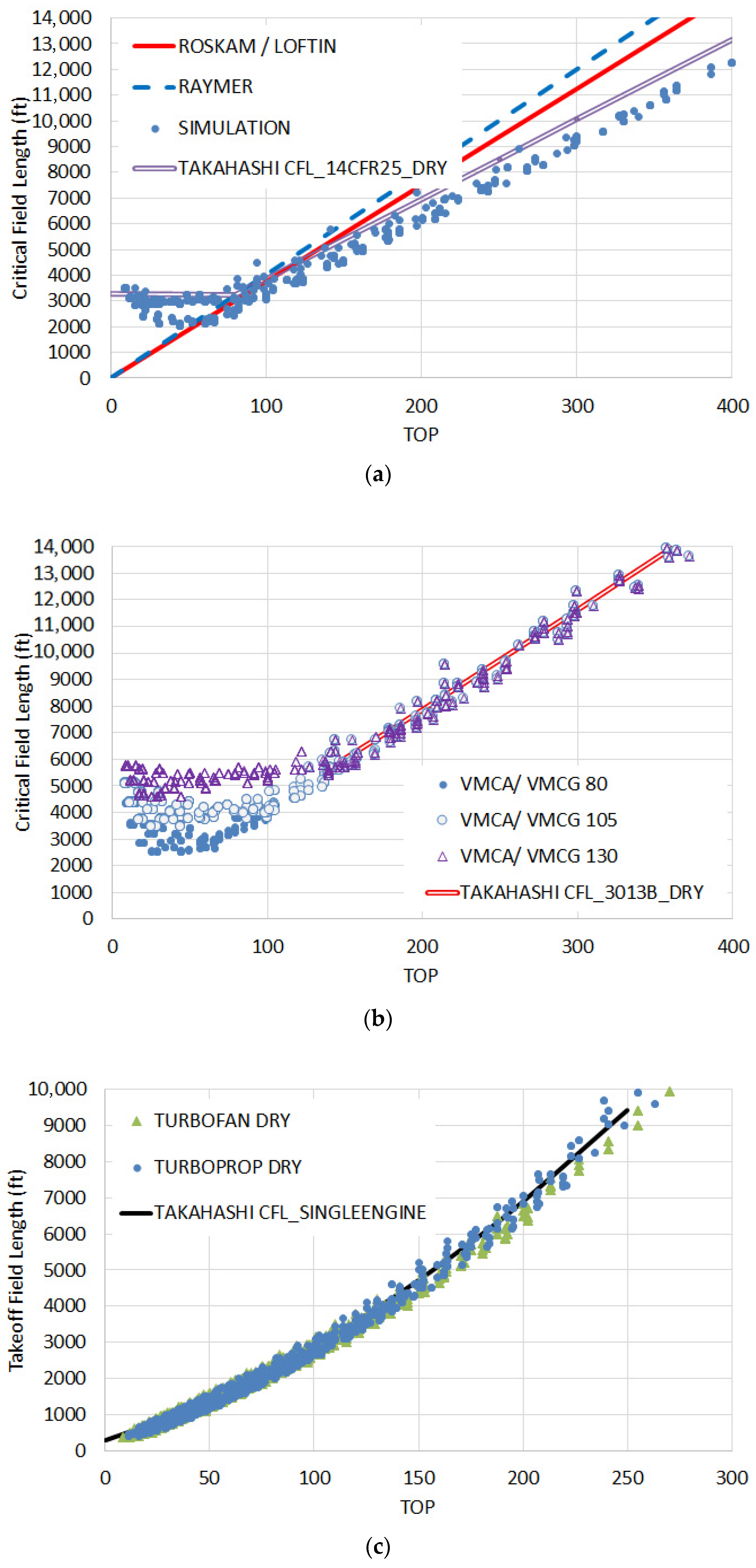
Figure 1 demonstrates that an empirically calibrated, physics-based time-step integration can more reliably predict speeds and distances to within 2 knots and 200 ft of the flight manual values across a wide range of dispatch weights, whereas Roskam’s equation tended to overpredict distances by over 1200 ft.

Since wet weather stop distances cannot take credit for improved braking traction, any revised empirical equations should be expanded to consider both dry and wet weather performance. In addition, to be suitable for a broad range of design projects, new empirical equations should be developed for a collection of diverse certification rules—14 CFR § 25 certified multi-engine transport category aircraft [31], MIL-STD-3013B rules multi-engine aircraft and MIL-STD-3013B rules single-engine aircraft [32]. Note that modern, European CS-25 rules are essentially identical to American 14 CFR § 25 rules [33].

The work shown here develops new empirical predictive equations based on a statistical model of ~7500 numerical time-step-integration simulations comprising a broad range of wing loading (W/S), thrust loading (T/W). It is consistent with modern civilian production aircraft flight manual data at a variety of dispatch weights. While the new equations are limited to sea-level/standard-day performance, they represent an improvement in prediction accuracy over all prior published empirical relations. In particular, these relationships highlight the impact minimum-control-speed limits and runway traction have on field performance. Use of these improved empirical equations, where appropriate, will reduce the “disconnect” which otherwise arises when inaccurate models are used to inform critical design decisions.

2. Prior Art

In 1934, Walter Diehl authored the seminal methods paper for take-off, NACA TR-450 [5]. Here, he derived a “comparatively simple method” to calculate the Take-Off-Ground-Roll, TOGR, in feet:

$$TOGR={\displaystyle \frac{K_S V_{TO}^2}{\left(\frac{T}{W}\right)}}$$

(1)

where V_TO is the take-off speed in ft/s, T is the static thrust in lbf, W is the gross weight of the aircraft in lbm and K_S is a coefficient which depends on the ratio of static to dynamic accelerating force taking into consideration the velocity lapse of thrust, aerodynamic drag and rolling resistance.

K.D. Wood, in his 1935 treatise “Technical Aerodynamics,” [6] basically re-iterated Diehl. He used basic kinematic equations based on static thrust, rolling resistance, lift-to-drag ratio at take-off, a prescribed thrust velocity-lapse rate, and a target take-off speed (nominally at CLmax, i.e., stall). He suggested that this method was appropriate to estimate all-engines operating take-off ground roll. Warner’s 1936 text on aircraft performance [7] expanded on Diehl. He suggested liftoff should occur at 125% of stall speed; and that this speed should be fed into Diehl’s equations. He included corrections for headwinds and ground effect.

Jones, in his 1939 textbook “Elements of Practical Aerodynamics,” [8] presented basic kinematic equations based on static thrust, rolling resistance, a prescribed thrust velocity-lapse rate, and a target take-off speed (nominally 105.4% stall speed). He too only estimated all-engines operating take-off ground roll.

Other period texts followed Diehl. For example, both Millikan’s 1941 [9] and Sherwood’s 1946 [10] texts directly referenced NACA TR-450 but provided no further insight.

Dwinell [11] basically followed Diehl but introduced the more modern concept of the characterizing propeller thrust lapse in terms of thrust coefficient. He specifically stated that his methods used an “arbitrarily assumed constant lift coefficient for the complete ground run” [11]. He ignored effects like landing gear, wing flap and cowl-flap drag “in order to maintain simplicity of analysis” [11]. Dwinell followed the emerging 14 CFR § 4 rule that the minimum take-off speed shall be no slower than 120% the stall speed [34]. He also described a highly simplified method to compute the AEO take-off distance to 50 ft AGL. To estimate the ground roll, he suggested replacing the 120% Vs liftoff speed with the airspeed which reflects the velocity which will produce the maximum angle of climb. He added the distance to 50 ft AGL, flown at a constant airspeed equal to the velocity for the maximum angle of climb as determined using a small-angle approximation.

The evergreen Perkins & Hage [12] moves us into the modern age. They find that the take-off distance to 50-AGL from “reliable flight test data” of a large number of airplanes is proportional to a Take-Off-Parameter, hence designated TOP:

$$TOP={\displaystyle \frac{\left(\frac{W}{Sref}\right)}{\left(\frac{T}{W}\right)C{L}_{max}}}$$

(2)

where TOP is the square of the take-off weight (W) divided by the wing area (Sref), static thrust of the propulsion with all engines operating (T) and the maximum lift coefficient (CLmax). The Perkins & Hage version of the equation substituted the actual lift coefficient at take-off as CL_TO~0.7CLmax, implying initial flight at 120% Vs. While Perkins & Hage show only a graphical correlation, we may fit their plot with the following equation to estimate the Take-Off Distance (TOD) to 50 ft AGL:

$$TO{D}_{PERKINS\&HAGE}\approx 28.5 TOP.$$

(3)

Corning’s 1960 [13] and K.D. Wood’s 1963 [14] aircraft design texts reiterate this relationship. Corning, in particular, noted that the correlation coefficient accurately models FAA 14 CFR § SR-422 (i.e., Boeing 707 and Douglas DC-8) certified jet aircraft [35].

Nicolai’s 1975 aircraft design text [15] added additional realism to a first principles model but loses all evidence of calibration with “real world” data. He is the earliest author to call out the variation in modeling ground rules between military multi-engine, civilian transport-category, and civilian general-aviation certification bases. He also included the rolling resistance of the tires in the take-off ground roll computation, added a transition maneuver, and concluded with an air-phase model to reach 50 ft AGL. Nicolai neither considered a rejected take-off or an engine failure in his analysis. Anderson’s widely used performance text closely followed Nicolai [16]. Unfortunately, neither of these AEO models are likely to accurately predict the OEI performance of certified multi-engine aircraft.

Perry [17] devised a 17-step process to estimate the Critical Field Length of a multi-engine aircraft flown to 1960s era civilian rules. He includes both all-engines-operating procedures, critical-engine failure on the ground as well as the rejected take-off scenario. He included a series of first-principles analytical and graphical semi-empirical methods to compute numbers for each element of his process. Torenbeek reiterates this approach in “Synthesis of Subsonic Aircraft Design.” [18] Author Takahashi uses Perry’s framework to write his time-step integrating simulation used to establish the underlying data for the novel empirical equations presented later in this paper [23].

Raymer’s early [19] and current [20] aircraft design texts presented charts derived from Perkins & Hage [12] and Loftin [30]. He suggests that the Balanced-Field-Length (BFL) is a strong function of TOP and a weak function of the number of engines. For a twin-engine jet-propelled with a 35 ft AGL air-phase height

$$BF{L}_{RAYMER}\approx 40 TOP.$$

(4)

However, Roskam’s performance text [21] presents Balanced-Field-Length as

$$BF{L}_{ROSKAM}\approx 37.5 TOP.$$

(5)

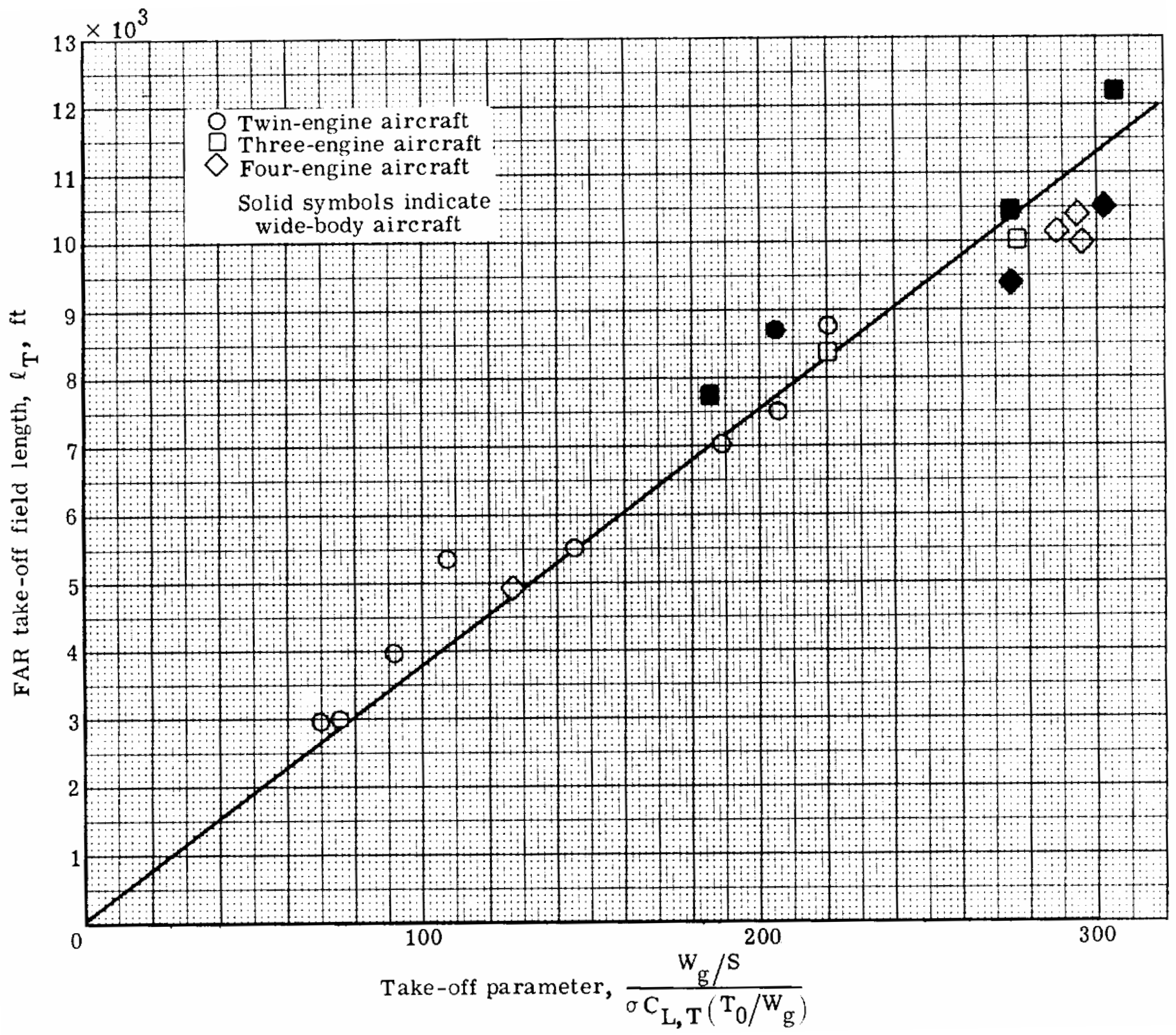
Roskam represents, in equation form, the precise correlation line found in Loftin’s NASA report; see Figure 2 [30].

Roskam’s equation neglects explicit impacts of thrust-asymmetry, rudder sizing and braking traction. Field performance depends upon wing loading, thrust loading and maximum lift coefficient; given enough wing and thrust it predicts vanishingly short distances. Conversely, real aircraft have a minimum critical field length distance which will be governed by Ground Minimum-Control Speed (VMCG) and/or Air Minimum-Control Speed (VMCA) limited accelerate–stop distances. No matter how large the engines or the wing, the critical field length cannot be shorter than the distance covered accelerating to the minimum decision speed (V1) and then stopping without the use of reverse thrust. In addition, referring back to the poor prediction of the A320 data (return to Figure 1a), we speculate that in the intervening years since Roskam and Loftin collated flight manual data, advances in automation and aircraft braking performance have substantially changed certified field performance distances.

3. Regulatory Basis for Certified Take-Off Distances

This section comprises an overview of the regulatory basis for certified take-off distances as excerpted from Takahashi’s book [22,23] and related conference papers [36,37,38,39,40,41,42]. Pilots and dispatchers use these distances, published in an Aircraft Flight Manual (Pilot’s Operating Handbook), to schedule operations.

3.1. Top-Level Differences Between MIL vs. Civilian Regulations

Military and civilian rules governing scheduled aircraft performance during take-off and landing differ. A complicated history explains the subtle nuances that divide 14 CFR § 25 and military rules aircraft from one another. Take-off regulations have been amended many times; this paper uses only the most modern 14 CFR § 25/CS-25 [31,33], MIL-STD-3013B [32] and 14 CFR § 23 [43] rule sets. These regulations are all “cousins” in that they share some common origins but have led separate lives for many years. The rules are architecturally identical but differ in detail. Military rules, which provide peace through strength, emphasize an ability to successfully plan and execute training operations at the “edge” of safe capability. Compared to civilian rules, they have greater margins of safety in some areas. Conversely, Civilian regulations focus on commercial reliability and safety when aircraft are not operated near the limits of their capabilities.

In a nutshell, the differences between FAA and MIL rules will lead to substantially different “book” performance values for an otherwise identical aircraft. Distinctly different empirical equations will need to be developed to assess multi-engine aircraft.

3.1.1. Multi-Engine Aircraft

While modern military multi-engine aircraft are controlled by the rules found in MIL-STD-3013B [32] and MIL-HDBK-1797 [44], civilian multi-engine transport category aircraft are functionally controlled by the regulations found in 14 CFR § 25 [31], 14 CFR § 91 [45] and 14 CFR § 121 [46]. Historically, military and civilian rules were identical; they both considered the take-off distance to be from brake-release to initial climb-out at 50 ft AGL. Today, 14 CFR § 25 certified distances consider the take-off air-phase to end when the aircraft is 35 ft AGL [31]. This change was introduced in 1957 under Special Civil Air Regulation 422, used to certify the Boeing 707 [35].

Additionally, 14 CFR § 91.117 places a speed limit not to exceed 250 knots below 10,000 ft for safe air-traffic management in terminal areas [45]. Military aircraft, as good neighbors, should be able to comply—at least under foreseeable training situations.

Civilian dispatch rules found in 14 CFR § 121.189 restrict operations by limiting dispatch to less than the highest certified weight [46]. This regulation also stipulates that aircraft must not be allowed to attempt to take-off unless: (1) the available runway for take-off (TODA) and accelerate–stop (ASDA) are in excess of the certified distances at the planned dispatch weight in light of current weather (outside air temperature, pressure altitude and winds), (2) the aircraft has sufficient one-engine inoperative climb performance to meet regulatory minimums and (3) the aircraft can actually overfly all known obstacles along the planned initial route with one-engine inoperative.

Other civilian multi-engine aircraft technical parameters (distances, speeds and climb gradients) are controlled by an intricate network of overlapping regulations: 14 CFR § 25.105, 14 CFR § 25.107, 14 CFR § 25.109, 14 CFR § 25.111, 14 CFR § 25.113, and 14 CFR § 25.115 [31], Functionally, civilian, and military rules differ in nuanced definition of cue speeds, allowable braking traction, use of reverse thrust and control margin for trim. These rule differences will be discussed in further detail later in this paper.

3.1.2. Single-Engine Aircraft

In 2016, the FAA revised 14 CFR § 23 certification regulations to replace prescriptive design requirements with “performance-based” airworthiness standards [43]. Consequently, current 14 CFR § 23 regulations are vague; they place the burden of specificity on other FAA documents like Advisory Circulars and Industry “best-practices.” Nonetheless, the single-engine take-off rules in MIL-STD-3013B mirror those in the new 14 CFR § 23.

Single-engine civilian aircraft certified under the most recent 14 CFR § 23 standards must conform to the broad rule which stipulates that the published take-off distance “includes the determination of ground roll and initial climb distance to 50 feet … above the take-off surface.” [43] Similarly, single-engine military aircraft, certified under MIL-3013B rules define take-off as the “phase of flight during which the air vehicle leaves the ground and enters aerodynamic and thrust-supported flight. It extends from starting engines to the start of the initial climb (50 ft above ground level)” [32].

3.2. MIL-STD-3013B Rules Take-Off Speeds and Distances

The take-off rules found in MIL-STD-3013B [32] are defined using specific, precise language.

The U.S. Military requires manufacturers to publish the maximum indicated speed to “refuse” to continue a take-off, Vref. Below this speed, the pilot can safely stop the aircraft on the available remaining runway. This applies equally to single-engine and multi-engine aircraft. For a multi-engine aircraft, performance demerits due to a failed engine are accounted for when establishing this speed.

The Stall Speed, Vs, is defined (per MIL-STD-1797A [44]) at 1-gee (i.e., where lift = weight) as the highest of: (1) the speed for steady, straight, and level flight at CLmax, the first local maximum of the curve of lift coefficient versus angle-of-attack which occurs as lift coefficient is increased from zero, (2) the speed at which uncommanded pitching, rolling, or yawing occurs, and (3) the speed at which intolerable buffet or structural vibration is encountered.

The Rotation Speed, Vrot, is the speed at which the aircraft transitions from ground run attitude to liftoff attitude; it must also be no slower than the minimum speed at which the controls, including vectored thrust, if applicable, can generate sufficient moments to initiate rotation. MIL-STD-3013B rules permit rotation to commence below VMCA provided that it is scheduled so that the aircraft otherwise meets lift-off and obstacle-clearance speed targets; the C-130J, when operated to MIL “maximum effort” rules is an example of such an aircraft [47].

The Liftoff Speed, Vlo, is defined as the speed at which the air vehicle leaves the ground for a specified altitude, weight, and configuration. It is the highest: (1) 110% of the out-of-ground effect-power-off stall speed, (2) the speed in-ground-effect where the lift equals weight when the aircraft is pitched to incipient tail-strike, (3) the minimum speed at which the air vehicle has no less than 0.5% unaccelerated climb gradient out-of-ground-effect at take-off power with the landing gear still extended, (4) the minimum speed having the longitudinal control power to initiate take-off rotation, (5) the speed that enables the aircraft to attain the obstacle clearance speed at or before the air vehicle clears a height of 50 ft AGL, and (6) any other minimum speeds based on flight control limitations.

The Obstacle Clearance Speed, VOBS, is defined as the flight path speed, with landing gear extended, at which the air vehicle clears 50 ft AGL during initial climb out, for a specified airfield altitude, weight, and configuration. It is the greater of: (1) 120% of the out-of-ground effect power-off stall speed with flaps in the take-off position, (2) the minimum speed at which the air vehicle has no less than 2.5% unaccelerated climb gradient potential out-of-ground-effect at take-off power with the landing gear retracted, and (3) any other minimum speeds based on flight control limitations (105% VMCG and 105% VMCA).

The lowest airspeed needed to achieve aerodynamic lateral-directional trim with one-engine inoperative (OEI) is known as the minimum-control speed. When establishing VMCG, MIL-STD-3013B allows credit for active nosewheel steering and up to 250-lbf rudder pedal force to achieve a directional torque balance. Once airborne, MIL-STD-3013B stipulates that, at or above VMCA, pilots shall without a change in aerodynamic configuration be able to neutralize lateral and directional torques after “a sudden asymmetric loss of thrust from the most critical” engine and “maintain straight flight throughout the climb-out” [34]. “The rudder pedal force required to maintain straight flight … shall not exceed 180 pounds” [34]. Moreover, “aileron control shall not exceed … 75 percent of available control power.” [34]. In addition, “the airplane may be banked up to 5 degrees away from the inoperative engine” [34].

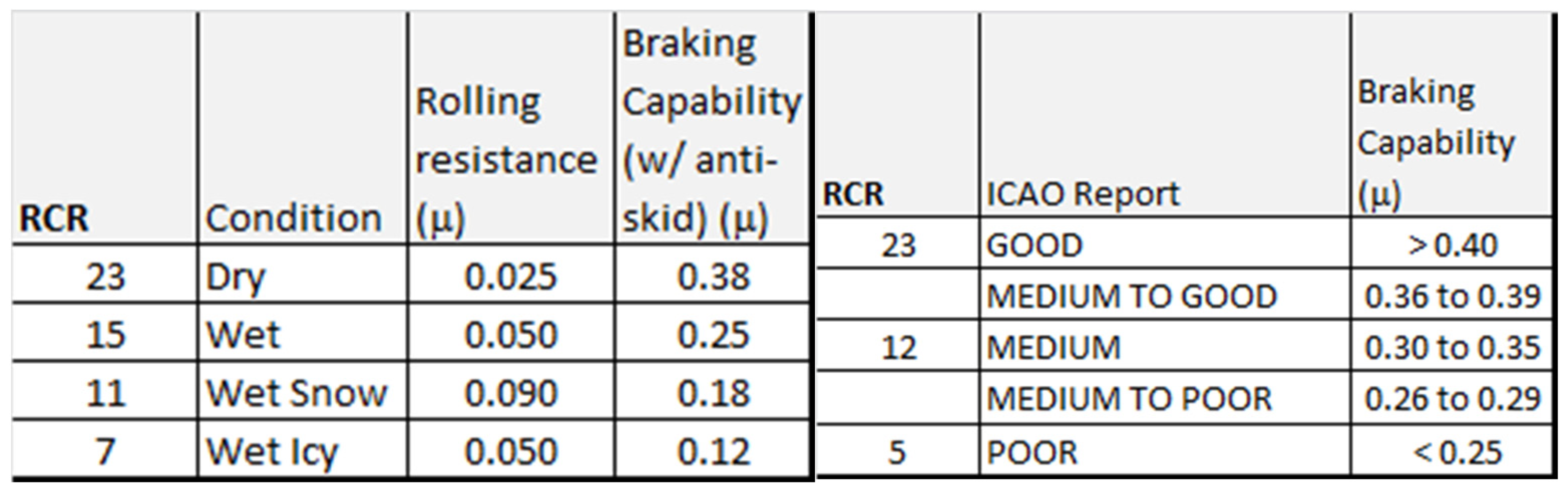
The US military characterizes dry and contaminated runway operations in terms of the Runway Condition Reading, RCR [34]. Civilian rules follow the International Civil Aviation Organization (ICAO) which also specifies qualitative and quantitative estimates of runway traction [48,49]. Section 3.5 of this paper will discuss these nuances in greater detail.

MIL-STD-3013B stipulates that critical field length is the greater of: (1) the basic take-off distance with all engines operating; (2) the accelerate–stop distance with the decision speed set to the published refusal speed (Vref) and (3) the accelerate–go distance with an engine failure timed so that the pilot first notices the engine failure just as the aircraft passes its refusal speed. MIL-STD-3013B requires the published distance to consider a delay between actual engine failure and the instant the pilot rejects the take-off.

3.3. Civilian 14 CFR § 25 Multi-Engine Take-Off Speeds and Distances

Civilian multi-engine rules differ in subtle but significant ways from MIL-STD-3013B; some involve nomenclature, others involve substance.

The FAA allows considerably more discretion with the definition of a stall, see advisory circular AC 25-7D [50]. The Stall Speed (Vs) defined by 14 CFR § 25 does not require substantiating flight test under 1-gee (lift = weight) conditions.

In civilian nomenclature, the take-off go/no-go speed is known as the decision speed, V1. Above this speed, the pilot commits to fly the aircraft with a failed engine because it can no longer stop within the remaining available runway. For a multi-engine aircraft, performance demerits due to a failed engine are accounted for when establishing this speed; the AC-25-7D advisory circular [50] stipulates a 1 s reaction time prior to posting V1 and distance credit for an additional 1 s lag after V1 before a rejected take-off can commence rather than the 3 s required for MIL-STD-3013B compliance [34].

Civilian rules Rotation Speed (VR) is the speed at which the pilot commands the transition from ground run to liftoff attitude. This speed must be fast enough to provide a safe speed margin between the resulting liftoff speed (VLOF), minimum-control-speeds (VMCG and 105% VMCA) and the minimum unstick speed (108% all-engines-operating, 104% VMU OEI). This rule allows the speed margin between VLOF and VMU to be reduced, and hence VR to be reduced, for airplanes where the minimum value of VMU is limited by the geometry of the airplane (i.e., ground contact of the tail of the airframe with the runway when the airplane is rotated to the take-off pitch angle). The idea behind this ruling is that “the geometry of the airplane provides protection against early or over-rotation beyond the safe liftoff pitch attitude at or near VMU, VR can be reduced without lowering the level of safety.” The FAA and EASA believe that “reducing VR reduces the take-off distance needed at the same weight or allows a higher weight (e.g., capability to carry more payload or fuel) at the same take-off distance” [51].

In civilian parlance, V2, is the “second segment climb speed;” basically the same as the military VOBS. It is defined as the flight path speed, with landing gear extended, at which the air vehicle clears 35 ft AGL during initial climb out, for a specified airfield altitude, weight, and configuration. For a turbine aircraft, it is the greater of (1) 113% of the out-of-ground effect power-off stall speed with flaps in the take-off position, (2) 110% of the published minimum control airspeed and (3) any other speed increments resulting from minimum rotation speed limitations. An aircraft rotated at VR should exceed the published V2 speed with AEO and just attain V2 with OEI.

Both civilian and military rules for critical field length are broadly similar. Regulation 14 CFR § 25.113 [31] adds one further constraint to the MIL-STD-3013B concept of critical field length; it defines CFL as the greater of: (1) 115% of the basic take-off distance with all engines operating; (2) the accelerate–stop distance with the decision speed set to the published V1 speed and (3) the accelerate–go distance with an engine failure timed so that the pilot first notices the engine failure just as the aircraft passes its V1 speed.

The regulatory minimum OEI climb performance governed by 14 CFR § 25.121 [31] differs from military rules (2.5%) [34]; civilian aircraft may not dispatch if their steady gradient of climb at the V2 speed with take-off flaps deployed and landing gear retracted does not exceed 2.4% for a two-engine configuration (more lenient than Military rules), 2.7% for a three-engine configuration or 3.0% for a four-engine configuration.

Because civilian rules do not allow credit for active nosewheel steering and have a lower (150-lbf) maximum allowable rudder pedal force limit, civilian minimum control ground speeds, VMCG, are slightly higher than the same aircraft would attain under military rules.

Since MIL-STD-3013B requires “at least 25% excess roll control power” they are “more stringent than the” corresponding civilian regulations which permit VMCA compliance with full aileron control [32]. Taken in light of the regulatory speed multipliers applied to VMCA, we see that MIL-STD-3013B requires considerably more stall speed margin during take-off and arguably more speed margin for OEI trim than civilian rules. This is consistent with the expectation that military transport aircraft operate in environments where engine failures are more likely than civilian aircraft.

3.4. Operations in Adverse Weather

The FAA does not specifically certify aircraft for take-off on an icy runway. However, they require aircraft performance engineers to consider the effects of icing. Icing conditions may degrade aircraft performance in two ways. First, engine power may be reduced when significant hot bleed air is diverted from the high-pressure compressor to feed cowl and leading-edge anti-ice systems. Second, ice accretion—even in the presence of a functioning anti-ice or de-ice system—may lead to an increase in stall speeds and a change in minimum-control-speed.

Conversely, MIL-STD-3013B [32] and MIL-STD-1797A [44] pay much less attention to the nuance of anti-ice and de-ice systems but require detailed landing distance estimates as well as procedures to be developed for operations on wet and contaminated runways. MIL-STD-3013B compliant aircraft, like the USAF C-130-J have distinct speed schedules which provide a proper margin of safety for operation under icing conditions, as well as field and climb performance estimates flown to the icing speed schedules that consider both thrust and braking degradation associated with anti-ice bleed schedules and slick and/or contaminated runways [45].

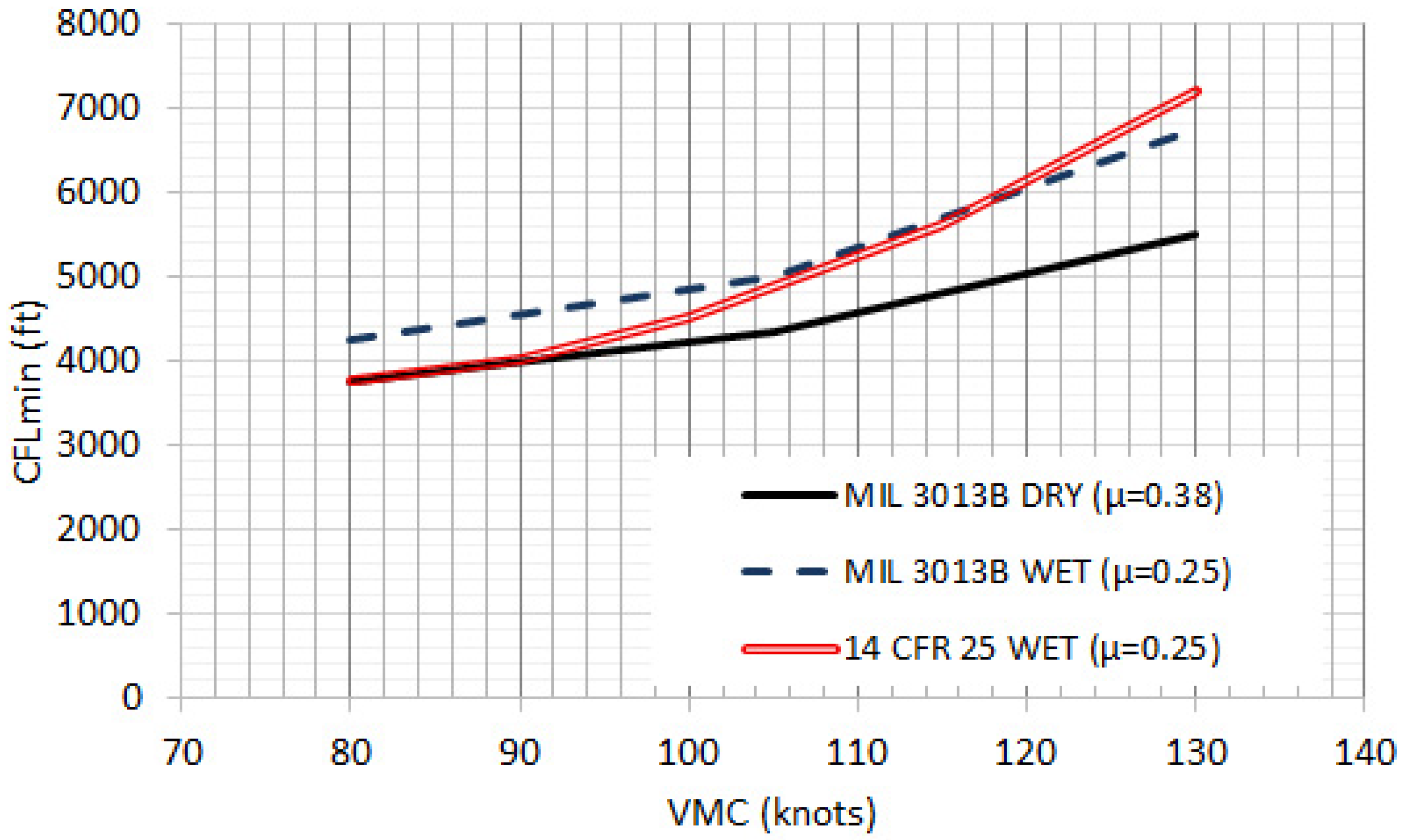
More specifically, in both the wet and the dry 14 CFR § 25 [31] permits credited braking performance at specified or ESDU 70,126 traction levels [52]. The FAA declines to provide any guidance regarding the traction available on icy or contaminated runways. If actual test data can document better stopping power than that implied by any default coefficient, the FAA will not force the manufacturer to use the pessimistic default values for stopping friction. Thus, many recent FAA-certified aircraft publish exceptionally short dry runway stopping distances associated with demonstrated braking at an effective μ > > 0.4; see Figure 3. Recall from Figure 1a, numerical simulations closely matched published A320 performance when the rejected take-off braking followed ESDU speed-dependent μ.

Both the U.S. Military and the ICAO characterize wet and contaminated runway operations in terms of the Runway Condition Reading, RCR. These qualitative and quantitative estimates of runway traction vary from RCR = 23 representing a standard hard-surface runway in the dry to RCR = 7 which represents a wet, icy runway; see Figure 4. MIL-STD-3013B specifies default values the engineers should use for computing rolling resistance and braking capability [32]. In each case the coefficient, μ, is defined as the ratio of the total retardation force of the wheels (either inherent in the tires and bearings, or due to the brakes) divided by the weight on wheels (the aircraft weight less any aerodynamic lift). Because FAA-certified dry braking friction may be significantly higher than allowed by MIL-STD-3013B, two otherwise identical aircraft will have different certified stopping distances.

3.5. Reverse Thrust Credit

Presently, the FAA forbids the use of thrust reversers when calculating the certified landing distance or take-off accelerate–stop distance [31,50]. In the United States, if reverse thrust is available, pilots will use it to save wear and tear on the brakes. In the European Union, community noise standards discourage the use of reverse thrust in normal operations. Alternatively, military rules explicitly permit reverse thrust. Thus, identical aircraft operating on civilian and military standards will have noticeably different certified stopping distances.

The reason why reverse thrust is taboo in certification has to do with interpretation of the nuance of the regulations. In 14 CFR § 25.125, the FAA stipulates that no braking credit may be granted for “any device is used that depends on the operation of any engine … if the landing distance would be noticeably increased when a landing is made with that engine inoperative.” [31]. However, it is common practice to interpret the phrase “means other than wheel brakes may be used to determine the accelerate–stop distance if that means … is such that exceptional skill is not required to control the airplane” as disallowing reverse thrust in the event of a critical engine failure even on four-engine aircraft [50].

3.6. Critical vs. Balanced Field Length

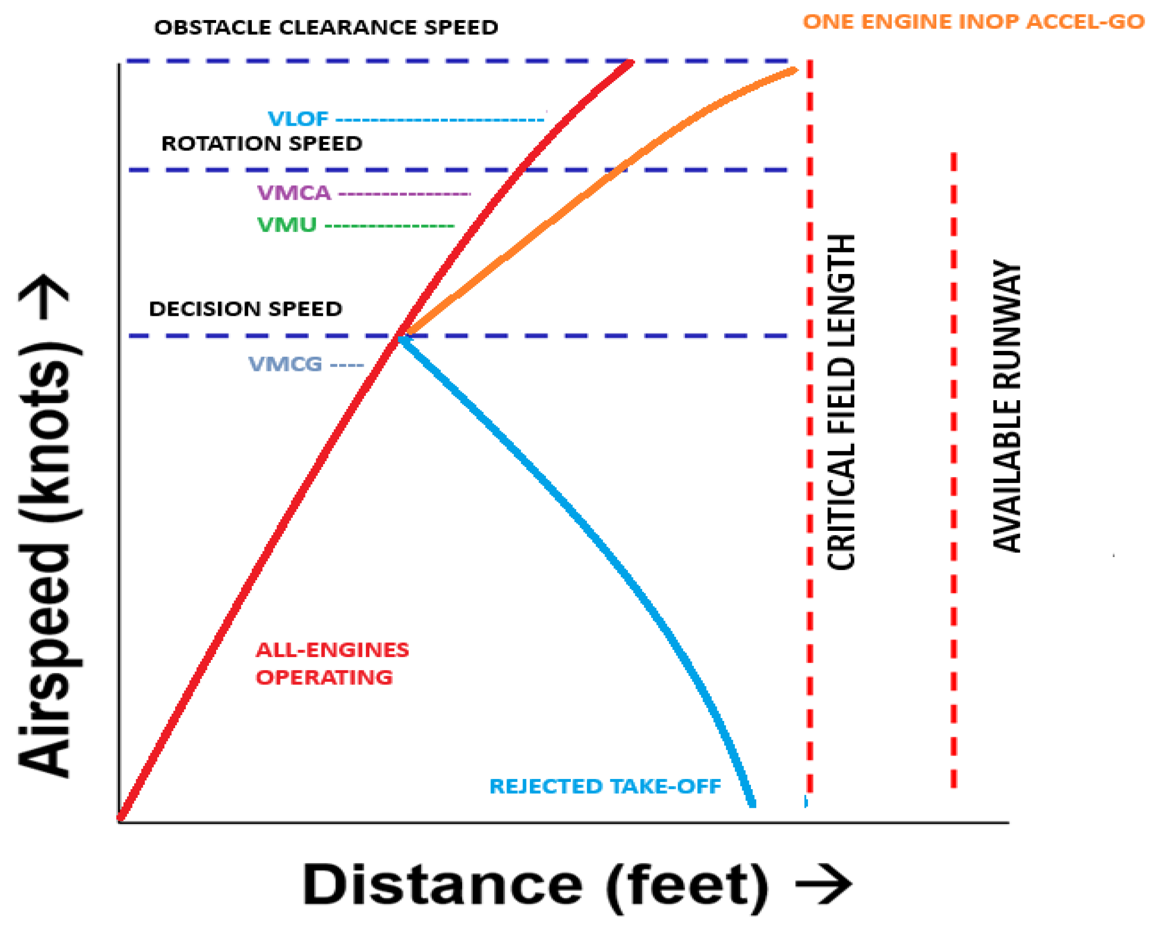
For multi-engine aircraft, the engineering team has the liberty to select the published decision speed (V1 under 14 CFR § 25 rules, Vref under MIL-STD-3013B rules). This go/no-go speed controls the entire take-off process. Above the decision speed, the pilot must continue the take-off process, following the scheduled rotation speed to enable the aircraft with one-engine inoperative to reach the published obstacle clearance speed (V2 under 14 CFR § 25 rules, VOBS under MIL-STD-3013B rules). Below the decision speed, a pilot faced with engine failure must reject the take-off and stop.

The take-off decision speed has physical limitations. First of all, the published speed (V1 or Vref) is closely associated with the airspeed at which the critical engine is assumed to fail. If the engine fails below VMCG, the pilot cannot maintain directional control; he must reject the take-off. Thus, VMCG sets an absolute lower floor to the decision speed.

Real-world aircraft will achieve the shortest accelerate–stop distances when VEF is set to VMCG; the longest accelerate–stop distances will be attained when the decision speed is set to VR. To prevent pre-destined doom of tail-strike, VR must exceed the minimum unstick speed, VMU. VMU is determined experimentally when a test pilot, after accelerating to a modest ground speed, aerodynamically tips the aircraft back onto its tail using full nose-up elevator control. The aircraft slowly accelerates under part power, dragging its tail down the runway, until the wheels just leave the ground. Supersonic aircraft, which may lack a distinct stall, despite having tall landing gear may not be able achieve minimum unstick below their published free-air Vs. Under 14 CFR § 25 rules, VR may not be less than 105% of minimum control airspeed (VMCA) or 105% of minimum unstick airspeed (VMU). As noted above, the C-130J is MIL-STD-3013B compliant in a “maximum effort” take-off even when rotated slightly slower than VMCA [45].

In practice, aircraft do not actually fly “balanced-field” procedures. In order to comply with regulatory requirements, it is rare that engineers can schedule the decision speed so that the rejected take-off accelerate–stop distance (ASD) exactly equals the one-engine inoperative accelerate–go distance (TOD_OEI); see Figure 5.

4. Numerical Simulation

This section comprises an overview of the kinematic simulations used herein. These are excerpted from Takahashi’s books [18,19] and earlier conference papers [36,37,38,39,40,41,42]. More extensive code fragments may be found in [19]. Time step integration is fixed at Δt = 0.050 s for all modes.

Recall that key aircraft speeds during both ground and flight phases of take-off are notated in terms of its equivalent airspeed, KEAS. Whereas, the kinetic energy of an aircraft is proportional to its true airspeed, KTAS. Therefore, numerical simulations (on non-standard and non-sea-level days and in the presence of winds) must simultaneously track aircraft speeds in terms of KEAS (for procedural control) as well as KTAS (to satisfy the equations of motion).

4.1. Overall Description of Take-Off Simulation

For take-off, the simulation must include modules to ensure that:

• The “accelerate–stop distance (ASD) must not exceed the length of the runway plus the length of any stopway” (the accelerate–stop distance available (ASDA)), and
• “Take-off distance (TOD) must not exceed the length of the runway plus the length of any clearway” (the take-off distance available (TODA))
• “Take-off (ground) run (TOGR) must not be greater than the length of the runway (TORA).”

For this study, we assume that ASDA, TODA, and TORA are equal. Thus, for multi-engine aircraft:

$$CF{L}_{MIL}=\max \left(TO{D_{50}}_{AEO} , TO{D}_{{50}_{OEI}}, AS{D}_{OEI}, AS{D}_{AEO}\right)$$

(6)

$$CF{L}_{FAA}=\max \left(115\% TO{D_{35}}_{AEO} , TO{D}_{30_{OEI}}, AS{D}_{OEI}, AS{D}_{AEO}\right)$$

(7)

For single-engine aircraft:

$$CF{L}_{SINGLE-ENGINE}=\max \left( TO{D}_{50}, ASD\right)$$

(8)

Similarly, the scheduled obstacle clearance speed is governed by one of the following:

$$VOB{S}_{MIL}=\max \left(120\% Vs, 105\% VMCA\right)$$

(9)

$$V{2}_{FAA}=\max \left(113\% Vs, 110\% VMCA\right)$$

(10)

$$V{50}_{FAA}=120\% Vs$$

(11)

4.2. Accelerate–Stop Simulation

For a rejected take-off, the simulation numerically integrates aircraft time and position history for two scenarios:

• When an engine fails at the most inopportune time (recognized by the pilot just as the aircraft reaches its critical decision speed) leading to a rejected take-off;
• When the pilot decides for any other reason to reject the take-off just as the aircraft reaches its critical decision speed.

In Scenario 1, we compute the total distance covered by the aircraft when it:

• Accelerates from a standing start with all engines operating to VEF;
• Accelerates from VEF to the highest speed reached during the rejected take-off, assuming the critical engine fails at VEF and the pilot takes the first action to reject the take-off at the decision speed;
• Traverses a distance representing a specified reaction time (2 to 3 s) at the decision speed;
• Decelerates with OEI, to come to a full stop.

In Scenario 2, we compute the total distance covered by the aircraft when it:

• Accelerates from a standing start with all engines operating to the highest speed reached during the rejected take-off, assuming the pilot takes the first action to reject the take-off at the decision speed;
• Traverses a distance representing a specified reaction time (2 to 3 s) at the decision speed;
• With AEO, it decelerates to a full stop on the runway.

Because braking action is a function of the weight on wheels, any residual lift developed by the wing reduces the effective weight on wheels, an airplane that lifts up at its ground incidence will have a longer stopping distance than one that develops downforce. In addition, the residual thrust of the engines at idle also contributes to the stopping distance. When calibrating the numerical simulations to published A320 flight performance [24], it became clear that its dry braking capability was considerably more powerful than μ = ~0.38. For A320, good calibration was attained when the dry weather braking capability matched the empirical model found in ESDU 71026 [52]. Conversely, MIL-STD-3013B requires official RCR-dependent values for braking friction; refer back to Figure 5.

4.3. Failed Engine Accelerate–Go Simulation

The failed engine accelerate–go simulation numerically integrates aircraft time and position history to simulate:

• Acceleration from a standing start with all engines operating to VE;
• From VEF to the decision speed, with OEI;
• From the decision speed to the scheduled rotation speed, with OEI;
• The pilot commands a nose-up attitude until the aircraft leaves the runway (where lift > weight);
• With OEI, allow the aircraft to climb until it reaches a height of 35 ft (civilian multi-engine rules) or 50 ft (military rules) AGL; the rotation speed must be selected so that the aircraft attains the scheduled obstacle clearance speed at the obstacle height.

The simulation tracks the OEI take-off ground roll distance (to the point where the wheels first leave the runway), TOGR, as well as the take-off distance to the obstacle height, TODR. It also tracks the speed at lift off, VLOF, in terms of indicated airspeed. It also computes climbing gradients.

4.4. All-Engines-Operating Take-Off Simulation

The AEO simulation computes the total distance covered by the aircraft when it:

• Accelerates from a standing start with AEO to the scheduled rotation speed;
• The pilot commands a nose-up attitude until the aircraft leaves the runway (where lift > weight);
• Climbs until it reaches the obstacle height (35 ft FAA multi-engine, 50 ft FAA single engine and MIL). Multi-engine aircraft are allowed to considerably exceed their scheduled obstacle-clearance speed, which is attained only in the event of engine failure during take-off.

The simulation tracks the AEO take-off ground roll (TOGR) as well as the take-off distance to the obstacle height, TOD.

4.5. Failed Engine Second Segment Climb Gradient

Estimate the climb gradient using the small-angle-approximation work-energy theorem as:

$$\gamma \approx {\displaystyle \frac{T-D}{W}}$$

(12)

where T is the thrust of the operating engines at the obstacle clearance speed and altitude of interest (400 ft above the runway elevation), D is the dimensional drag of the airframe with take-off flaps deployed, gear retracted including the drag of the inoperative engine and W is the analysis weight.

4.6. Parametric Sensitivies

Using an earlier version of the take-off time-step integrating code, following 14 CFR § 25 civilian rules, author Takahashi along with collaborators Wood & Bays studied the sensitivity of CFL to many parameters [39,40,41]. While weight and thrust are the dominant factors, procedural and dispatch parameter variability also impact take-off performance.

Because there is neither a Federal civilian nor a Military requirement for manufacturers to document “standardized procedures” for operations, aircraft flight manuals may be quite vague regarding piloting technique. We found that this lack of clarity has a potentially drastic effect on actual takeoff distances. In particular, slight changes in take-off pitch attitude and rotation pitch rate have profound impacts on the accelerate–go distance. Brake effectiveness (both μ and the effectiveness of lift-dump which influences weight-on-wheels) impact accelerate–stop distances. Thus, slight deviations in takeoff procedures and assumed braking effectiveness significantly impacted published field performance.

While real-world aircraft are expected to dispatch under a broad envelope of atmospheric conditions, conceptual design performance is typically computed only under sea-level/standard-day conditions. In the past some empiricism incorporated simple altitude dependence through a (σ) “sigma altitude” correction; refer back to Loftin’s Take-off Parameter in Figure 2. No prior empirical method prescribed a means to study the effects of temperature deviation. Because modern engines with thrust limiting (i.e., flat-rated thrust to ISA + 15 °C or flat-rated thrust to 50 KEAS) do not follow a “sigma altitude” lapse rate, this work focuses entirely on developing sea-level/standard-day regressions based on a sea-level/standard-day propulsion model. Author Takahashi has studied the effects of programmable lapse-rate on 14 CFR § 25 CFL and documented the effects disparate AEO and OEI programmed lapse rates (including a “throttle push” upon sensed engine failure) have upon certified performance [42].

5. Development of New Empirical Models from Numerical Simulation

Empirical model development begins with the selection of relevant dependent and independent variables. It continues with the collection of calibration and validation data. It then performs a statistical regression based upon a broad range of data spanning the design space the method is expected to support.

The broadest independent variables include the wing loading (W/S), static-thrust-to-weight ratio (T/W) with all-engines-operating and the maximum lift coefficient (CLmax) with the aircraft high-lift system in the take-off configuration. We find excellent correlation if we continue to follow tradition and correlate the relevant dependent variable (the CFL) with Perkins & Hage’s “Take-Off Parameter.” In some circumstances, we find a need to introduce one further independent parameter, the minimum control speed (VMC), in order to facilitate better correlation.

Because prior work noted the sensitivity of distance to timing and procedure, the choice of certifying authority must also be considered as a “independent” design variable. Consequently, the decision-tree within the simulation has been customized as appropriate. FAA rules multi-engine certified performance, MIL-3013B rules scheduled performance and single-engine MIL-3013B rules flight are modeled using related, but dedicated simulations.

Initial calibration with Airbus A320 flight-manual data was made for dispatch at sea-level/standard-day conditions under still winds following the modern 14 CFR § 25; refer back to Figure 1 [24]. The engine model had a natural velocity lapse; take-off static thrust occurs where N1, N2 and T4 are all at their respective rated maximums. CLmax was chosen to match published V2 speeds with no further airspeed calibrations; in other words, TAS = CAS = EAS. Braking μ matched ESDU 70126 [52]. Unbraked wheels had μ = 0.0025. Weight on wheels was a function of dispatch weight offset by aerodynamic lift: CL0 = 0.3; dCL/dα~0.1177/(1 + 2.385/ARe); CD = CD0 + CL²/(π ARe); ARe includes a ground-effect increment. Lift-dump spoilers, when deployed, add additional drag and cancel all aerodynamic lift.

5.1. FAA and MIL Rules Multi-Engine Performance

In order to determine a general basis for new statistical models, we ran the take-off simulation code over a wide range of aircraft configurations and conditions.

• W/S from 190-lbf/ft² to 38-lbf/ft²;
• AR from 4 to 12;
• CLmax of 1.25, 1.9 and 2.2;
• T/W from 0.15 to 2.2. (considering a configuration with two turbofan engines, nominal static thrust rating and associated lapse rates at sea-level/standard-day);
• VMCA = VMCG = 80 through 130 KIAS;
• Maximum ground angle-of-attack, α_tailstrike = 10, 14, 18-deg;
• CL0 on the ground, take-off flaps deployed = 0.3;
• ΔCL for deployed lift dump spoilers = −0.3;
• CD0 in flight = 0.0225;
• ΔCD0 for landing gear = 0.0070;
• ΔCD0 for deployed lift dump spoilers = 0.0250;
• μ = 0.025 for unbraked wheel rolling resistance dry, 0.050 wet;
• ESDU speed-dependent braking traction for 14 CFR § 25 dry; μ = 0.38 MIL-STD-3013B dry, μ = 0.25 wet;
• Engine Failure Reaction Time: 14 CFR § 25 2 s; MIL-STD-3013B 3 s;
• Rejected Take-Off Lift Dump/Brake Application Time: 1 s;
• Pitch-up rate for T/O rotation: dα/dt = 4 deg/s.

Valid simulations comprise solutions where T/W < 1, CFL < 14,000 ft and OEI second segment gradient > 2.4% (14 CFR § 25) > 2.5% (MIL-STD-3013B). When given A320-type values, the simulation closely matches scheduled performance; refer back to Figure 1.

5.2. FAA and MIL Rules Single-Engine Performance

In order to determine a general basis for the new statistical model, we ran the take-off simulation code over a wide range of aircraft configurations and conditions. The simulation was run over a full-factorial design space embodying the following:

• W/S from 10-lbf/ft² to 75-lbf/ft²;
• AR from 3 to 12;
• CLmax of 1.0, 1.4 and 1.8 with associated CL0 = 0.0, 0.2 and 0.4;
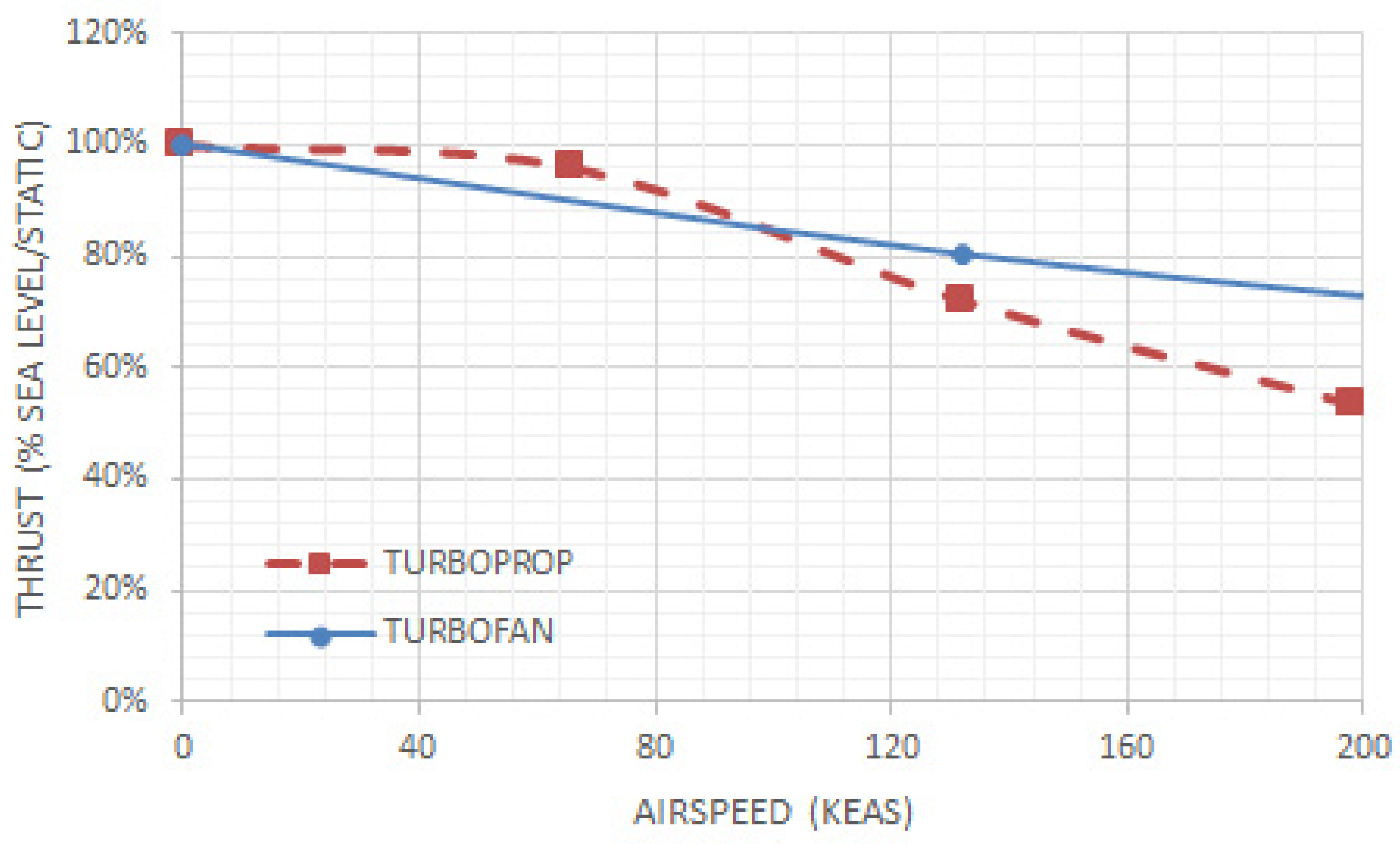
• T/W from 0.15 to 0.70. We consider the speed/thrust lapse rate of a turboprop engine as well as a medium bypass ratio turbofan engine; see Figure 6. This lapse is based upon data normalized from vendor supplied sea-level/standard-day cycle decks;
• Maximum ground angle-of-attack, α_tailstrike = 10, 14, 18-deg;
• CD0 in flight = 0.0250;
• ΔCD0 for landing gear = 0.0100;
• μ = 0.025 for unbraked wheel rolling resistance dry, 0.050 wet;
• μ = 0.38 braking traction in the dry or a μ = 0.25 for braking in the wet;
• Rejected Take-Off Refusal Speed at Scheduled Rotation Speed;
• Rejected Take-Off Brake Application Time: 1 s;
• Pitch-up rate for T/O rotation: dα/dt = 4-deg/s.

Valid simulations comprise solutions where second segment gradient > 2.5% (MIL rules), 4% (14 CFR § 23 high-speed and/or type 3 or 4 turboprop) or 8.3% (14 CFR § 23 piston prop/turboprop) [33,34,40,50].

6. Discussion

Our statistical basis consists of more than 1400 valid solutions for 14 CFR § 25 multi-engine take-off, 3600 valid solutions for MIL-STD-3013B rules multi-engine take-off and 2500 valid solutions for single-engine take-off. They comprise operations in wet and dry and inherently include VMCA, VMCG and VMU (i.e., tail strike) limited performance cases. All simulations were performed assuming dispatch under sea-level/standard day conditions.

Simulation data correlates closely when CFL is plotted as a function of Perkins & Hage’s TOP parameter, recall Equation (2) [8]. Figure 7 compares the multi-engine simulation to Roskam and Raymer for dry weather operations [15,16,17]. Figure 7a shows that Roskam’s and Raymer’s formulae are extremely pessimistic, assuming modern 14 CFR § 25 rules and ESDU dry weather braking; it suggests the need for a more accurate, revised empirical fit. Figure 7b shows that Roskam’s and Raymer’s formulae is generally on-point for MIL-STD-3013B dry weather take-off rules but fails to capture the minimum CFL (accel-stop limitations) governed by the fact that VMCG imposes a floor upon the decision speed. Finally, Figure 7c reveals a more quadratic, less linear, trend associated with single-engine operations.

We may define a best, “conservative” fit of the simulation data. For Civilian rules in the dry (data in Figure 7a), we obtain:

$$CF{L}_{14CFR25\_DRY}=\max \left( 750+31 TOP, 3300 \right)$$

(13)

Compared to the classic Roskam equation, this formula predicts improved performance for TOP > ~100 and inferior performance for TOP < ~100 where the aircraft will be VMCA and/or VMCG limited.

We may turn to

Table 2. Accuracy of Takahashi’s revised method to predict the certified flight manual critical field length for sea-level/standard-day dispatch near MTOW.

Aircraft	Flap Settings	Dispatch Weight (lbm)	Handbook CFL (ft)	TOP	Equation (13) CFL (ft)	Error
A340-200	CONF 2	553,865	9850	294	9864	<1% error
A350-1000	CONF 1 + F	708,722	9500	297	9957	5% pessimistic
B777-200	FLAPS 20	750,000	9200	280	9430	2.5% pessimistic
B767-400	FLAPS 5	450,000	10,800	332	11,042	2.2% pessimistic
A320-200	CONF 1 + F	170,000	6500	193	6733	3.6% pessimistic
E190-E2	FLAP 4	121,220	5089	168	5958	17% pessimistic

to examine how well the new, empirical formula based upon parametric sweeps matches published flight manual data. While simulation timings and braking traction were initially calibrated to best match Airbus A320-200 data, no further attempt was made to “curve fit” production aircraft performance. Table 2 demonstrates less than 5% predictive error for most modern aircraft when analyzed near their respective MTOW. The E190-E2 remains an outlier, where the revised method predicts CFL is nearly 900 ft longer than published. The discrepancy may arise if its propulsion system includes a programmed lapse rate that derates its published sea-level static thrust.

Next, let us look at Figure 8 to understand the ability of this new method to estimate take-off performance at lighter weights. We can see here that Raymer [19,20] and Roskam’s [21] legacy equations predict performance substantially pessimistic of many other actual, certified aircraft [24,25,26,27,28,29]. For example, the Airbus A350-1000 (Sref = 4998 ft²) has CFL = 7200 ft for dispatch at a 270 metric ton sea-level/standard-day dispatch (W = 594,270-lbm) with flaps set to CONF 1 + F (CLmax~1.74) [26]. Based on a 97,000 lbf rated sea-level/standard day static thrust of each of its engines, TOP = 209. Equation (13) predicts CFL = 7229 ft (29 ft pessimistic). Roskam predicts 7837 ft (~9% pessimistic). Raymer predicts 8360 ft (~16% pessimistic). Similarly, the B777-200 (Sref = 4605 ft²) has CFL = 9200 ft for dispatch at W = 750,0000 lbm sea-level/standard-day with FLAPS20 (CLmax = 1.99) [27]. Based on a 110,000 lbf rated sea-level/standard day static thrust of each of its engines, TOP = 280. Equation (13) predicts CFL = 9430 ft (230 ft pessimistic). Roskam predicts 10,500 ft (~14% pessimistic). Raymer predicts 11,200 ft (~21% pessimistic).

Thus, we can see that this new, simulation-based empirical relationship, using ESDU braking capability, is a much better predictor of contemporary certified aircraft performance. It works well at MTOW and when used to analyze dispatch at reduced weights for operations on shorter runways.

Having established the credibility of the simulation-based approach, we now derive from the data found in Figure 7b a relationship for MIL-STD-3013B operational rules performance in the dry. We obtain:

$$CF{L}_{3013B\_DRY}=\max \left(250+38 TOP, CFLmi{n}_{3013B\_DRY}\right)$$

(14)

where (refer to Figure 9) the minimum-control speed floor on decision speed limits CFL to a distance no-less-than:

$$CF{Lmin}_{3013B\_DRY}\approx 5525-58VMCG+0.44{VMCG}^2$$

(15)

Next, we turn to a study of wet weather performance. While the FAA allows “factored” dry runway data for dispatch planning in the wet, EASA wants realistic contaminated runway data [33,35]. Consequently, we run both the civilian and MIL rules simulations with μ = 0.25 to reflect RCR = 15 expected braking performance with anti-skid [34].

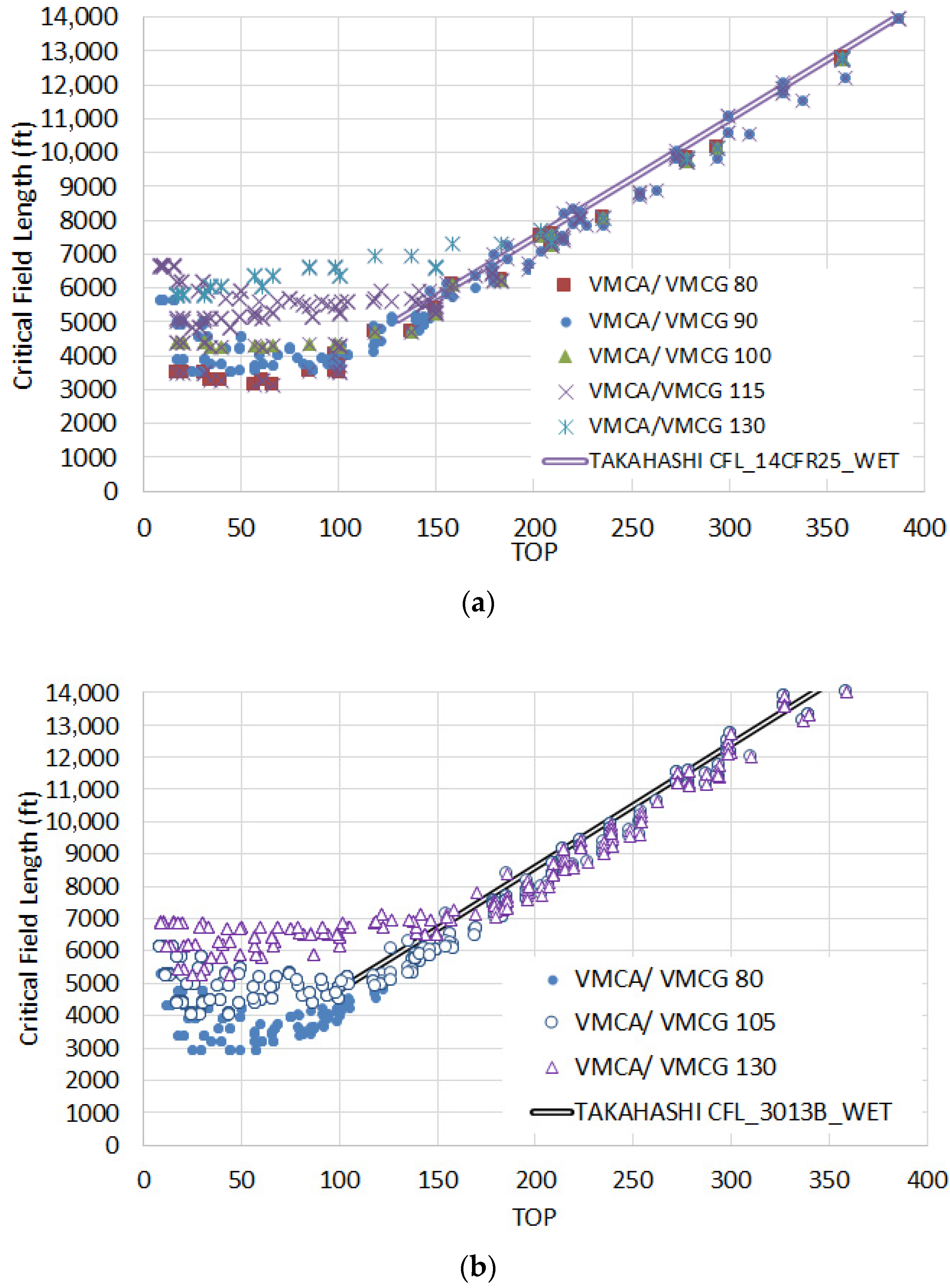
The complete statistical survey for μ = 0.25 wet braking correlates nicely as a function of TOP; see Figure 10. Figure 10a represents distances estimated following modern 14 CFR § 25 rules: Figure 10b for modern MIL-STD-3013B rules and Figure 10c for single-engine operations. As with the dry, multi-engine aircraft performance in the wet can be approximated with a linear function of TOP limited by a VMCG-dependent floor. Single-engine performance may be approximated with a quadratic fit.

Our best, “conservative” fit of the data presented as Figure 10a (civilian rules) is:

$$CF{L}_{14CFR25\_WET}=\max \left(500+35 TOP, CFLmi{n}_{14CFR25\_WET}\right)$$

(16)

where VMCG limits (refer back to Figure 9) distance to not-less-than:

$$CF{Lmin}_{14CFR25\_WET}\approx 7700-125VMCG+0.928{VMCG}^2$$

(17)

In other words, to guarantee that civilian rules aircraft have sufficient wet weather take-off performance to operate from a shorter runway like KDCA (TODA = TORA = ASDA = 6869 ft) we need to design an aircraft with VMCA < ~125 KIAS. For operational utility at runway 13L/13R at KMDW (where TODA = TORA = ASDA = 5141 ft), we would need VMCA < 105 KIAS.

MIL-STD-3013B rules simulations (see Figure 10b) support the following best “conservative” fit of the simulation:

$$CF{L}_{3013B\_WET}=\max \left(1000+38 TOP, CFLmi{n}_{3013B\_WET}\right)$$

(18)

where

$$CF{Lmin}_{3013B\_WET}\approx 8570-118\mathrm{V}\mathrm{M}\mathrm{C}\mathrm{G}+0.8{\mathrm{V}\mathrm{M}\mathrm{C}\mathrm{G}}^2$$

(19)

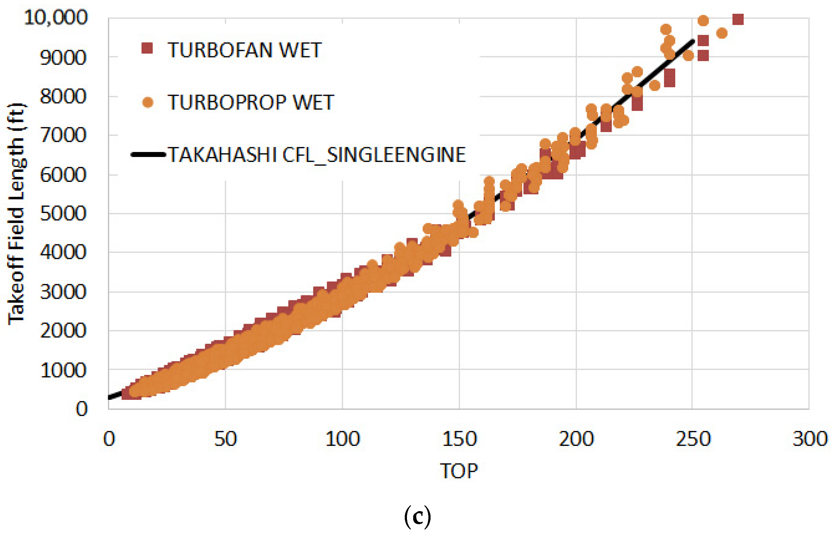
And finally, for single-engine aircraft, we can determine a “conservative” fit of the simulation data for operations in the dry and wet (shown in Figure 7c and Figure 10c, respectively) by:

$$CF{L}_{SINGLEENGINE}=300+19 TOP+0.07 TO{P}^2$$

(20)

Because the distance traveled through take-off rotation and flight to 50 ft AGL typically exceeds even the wet weather stop distance (assuming μ = 0.25), the statistical fit does not need to distinguish between operations on dry and wet runways.

7. Summary and Conclusions

From this deeper analysis of a wide range of conventionally configured transport aircraft, we see that take-off performance using a calibrated numerical simulation reveals issues with legacy statistical approaches. The most critical issue among these being that the equations have become inaccurate when applied to modern aircraft.

Consequently, this paper develops a collection of new empirical formulae to estimate sea-level/standard-day take-off performance for conventionally configured aircraft under a variety of certification bases (MIL-STD-3013B, multi-engine 14 CFR § 25 and single-engine 14 CFR § 23) tailored to wet and dry weather operations. They produce substantially different estimates than do the legacy equations.

The new equations are derived from a statistical analysis of a parametrically varied time-step integrating simulation calibrated to modern flight manual data. The statistical basis covered a wide range of thrust loadings (0.15 < T/W < 1+) and wing loadings (38 < W/S < 190-lbm/ft² for multi-engine aircraft, 10 < W/S < 75-lbm/ft² for single-engine aircraft). The basis also spans a broad range of aspect ratio (3 < AR < 12), implied high-lift system configurations (through variation in CLmax), landing gear height (through variation in α_tail-strike) and tail size (through variation in minimum-control speeds). In many cases, the critical field length is limited by VMC; in other cases, critical field length is limited by tail strike. The basis data is broad enough to cover a wide range of conventional and unconventional aerodynamic configurations, provided that they are operated according to standard practice.

Despite the strong statistical basis, the reader should remember that these empirical functions are only approximate. When used as intended, they typically predict “certified” handbook distances within 5%. However, these methods are inappropriate to analyze aircraft flown with atypical procedures; for example, STOL rules turboprops flown on a non-standard speed schedule like a “maximum-effort” take-off on a C-130J. They are equally unsuitable to evaluate configurations which feature unusual engine-inoperative aerodynamics (for example, distributed propulsion STOL aircraft with blown wings). Conceptual design level field performance for those aircraft must be assessed using a bespoke time-step integrating simulation.