Research on Sliding-Window Batch Processing Orbit Determination Algorithm for Satellite-to-Satellite Tracking

Abstract

In response to the increasing demand for high-precision navigation of satellites operating in the cislunar space, this study introduces an onboard orbit determination algorithm considering both convergence and computational efficiency, referred to as the Sliding-Window Batch Processing (SWBP) algorithm. This algorithm combines the strengths of data batch processing and the sequential processing algorithm, utilizing measurement data from multiple historical and current epochs to update the orbit state of the current epoch. This algorithm facilitates rapid convergence in orbit determination, even in instances where the initial orbit error is large. The SWBP algorithm has been used to evaluate the navigation performance in the Distant Retrograde Orbit (DRO) and the Earth–Moon transfer orbit. The scenario involves a low-Earth-orbit (LEO) satellite establishing satellite-to-satellite tracking (SST) links with both a DRO satellite and an Earth–Moon transfer satellite. The LEO satellite can determine its orbit accurately by receiving GNSS signals. The experiments show that the DRO satellite achieves an orbit determination accuracy of 100 m within 100 h under an initial position error of 500 km, and the transfer orbit satellite reaches an orbit determination accuracy of 600 m within 3.5 h under an initial position error of 100 km. When the Earth–Moon transfer satellite exhibits a large initial orbital error (on the order of hundreds of kilometers) or the LEO satellite’s positional accuracy is degraded, the SWBP algorithm demonstrates superior convergence speed and precision in orbit determination compared to the Extended Kalman Filter (EKF). This confirms the proposed algorithm’s capability to handle complex orbital determination scenarios effectively.

1. Introduction

In recent years, lunar exploration activities have significantly increased, with the Moon emerging as a strategic priority for major space agencies worldwide [1,2,3,4,5]. This surge in exploration is propelled by significant advancements in space technology, leading to a diversification and increased frequency of space missions. However, these developments present new challenges to conventional methods of satellite orbit determination. Traditionally, orbit determination has relied on ground-based systems [6], which exhibit several limitations. Firstly, the link between satellites and ground stations can be easily disrupted, necessitating that satellites remain within the coverage range of ground stations for extended periods to achieve accurate orbit determination. Secondly, ground-based methods lack real-time capabilities, resulting in slow updates of measurement data. Furthermore, ground-based orbit determination usually requires the cooperative work of multiple globally distributed ground stations, which involves high-frequency cross-country collaboration and ongoing equipment maintenance at a high cost. Lastly, the accuracy of observations from ground stations is often compromised by weather conditions, further impacting orbit determination precision [7]. Looking ahead, the anticipated increase in the number of satellites will render ground-based orbit determination increasingly challenging and burdensome, particularly in supporting large-scale Earth–Moon space activities.

Given the limitations of ground-based measurement systems, some researchers [8,9,10] have proposed the implementation of space-based orbit determination methodologies, establishing inter-satellite links between satellites to obtain measurement data. Reference [11] conducted experiments integrating inter-satellite link and ground tracking data into traditional GNSS solutions, achieving improvements in orbit determination accuracy of 64.9% over the GNSS-only solution. The article suggests that compared to ground observations, inter-satellite links contribute more significantly to satellite precise orbit determination (POD) due to their superior observation geometry.

Currently, space-based orbit determination technology predominantly employs relay satellites or navigation satellites as measurement stations in space. These measurement stations establish links with other satellites to acquire measurement data. The collected measurement data are integrated with orbital dynamics, enabling the application of an orbit determination algorithm to ascertain the orbit of the corresponding satellites. This orbit determination approach imposes stringent requirements regarding the real-time capabilities, robustness, and accuracy of onboard navigation calculations. ‘Real-time’ refers to the time synchronization between measurement data acquisition and orbit solving under the current limitations of onboard computing resources. ‘Robustness’ refers to the capacity to maintain stable convergence of the orbit determination process, even when the initial orbital error is large. High accuracy necessitates that the precision of inter-satellite link orbit determination meets or exceeds that of traditional ground-based orbit determination methods. To ensure real-time performance, filtering techniques are typically employed for orbit determination, while batch processing methods are generally utilized to guarantee convergence. The filtering techniques examined in the existing literature primarily include the Extended Kalman Filter (EKF) [12], evolutionary methods for EKF, and the Unscented Kalman Filter (UKF). The EKF algorithm is generally sub-optimal and is applicable only in cases of relatively mild nonlinearity [13]. Reference [14] analyzes POD with batch processing and the EKF based on actual measurement data from next-generation BDS satellites and proposes an EKF with a priori device delay constraints. The results show that when faced with more obvious nonlinearity or larger initial orbit errors, the POD using only inter-satellite links cannot converge when using EKF for orbit determination. In response to the shortcomings of the EKF, a number of scholars have proposed a series of evolutionary methods for the EKF to improve its performance. The SRIF method proposed by researchers at JPL (Bierman, 1977) [15], for instance, uses the household orthogonal transform to update the measurement and time in filtering recursive calculations, which improves the numerical accuracy and stability of the filtering. Yang et al. proposed an adaptive robust filtering method for satellite POD [16], which can effectively reduce the influence of observation and dynamic information anomalies on orbit state estimation. However, the above filtering methods still share the same key problem of being sensitive to the initial state of the satellite orbit. Moreover, the cold start of real-time filtering POD requires a long convergence time [17]. The UKF demonstrates superior performance for general nonlinear systems. However, based on the orbit determination results of the TURKSAT 5B satellite, Reference [18] shows that its improvement effect is limited compared to the EKF, and it necessitates a greater number of sampling points, leading to increased computational demands. The batch processing method requires a certain duration for data accumulation and is typically employed for post-processing on the ground, rendering it unsuitable for real-time computations aboard satellites.

In this paper, a scenario of space-based orbit determination is shown in Figure 1, where a low-Earth-orbit (LEO) satellite is equipped with a Global Navigation Satellite System (GNSS) receiver to facilitate real-time orbit determination and timing onboard. The Earth–Moon satellite acquires measurement data by establishing a link with the LEO satellite. Based on this scenario, an orbit determination algorithm that combines batch processing and sequential estimation is proposed. The algorithm can ensure convergence and orbit determination accuracy under real-time calculation. This method is called the Sliding-Window Batch Processing (SWBP) method, which means that a window contains several consecutive epochs, and all the measurement data from this batch of epochs is used to update the estimated state of the last epoch’s orbit. After completing the processing of this batch of data, the window slides forward in a certain number of steps and the process is repeated after introducing new measurements. The algorithm proposed in this paper is essentially still based on sequential estimation, but it considers the historical accumulation of multiple measurement data, thus ensuring the convergence of the orbit determination process in the case of large initial orbit errors.

This paper first introduces the basic equations of the inter-satellite dual one-way measurement model, followed by the dynamic equations of satellite motion and the detailed derivation of the innovative algorithm in this paper. In Section 4, the performance of the proposed algorithm is tested by performing simulated data simulation and actual onboard data testing in the above space-based orbit determination scenario. The experiments show that this algorithm effectively improves the stability, convergence speed, and accuracy of orbit determination calculations.

2. Inter-Satellite Link Measurement Model

The LEO satellite and Earth–Moon satellite establish dual one-way ranging links to obtain bidirectional ranging values [19]. The inter-satellite ranging value records the time difference between sending signals from the transmitting end and receiving signals from the receiving end, which not only includes the distance information between two satellites, but also includes factors such as clock offset, equipment delays, and measurement thermal noise [20,21]. These dual one-way ranging data are not directly used for orbit determination. By summing up the two ranging data, clock offset information can be eliminated and distance information can be retained, thus obtaining the orbit determination equation; subtracting two ranging values can eliminate the influence of distance, preserve clock offset information, and yield the time synchronization equation. The combined equation achieves the decoupling of distance and clock offset, and thus participates in the orbit determination process.

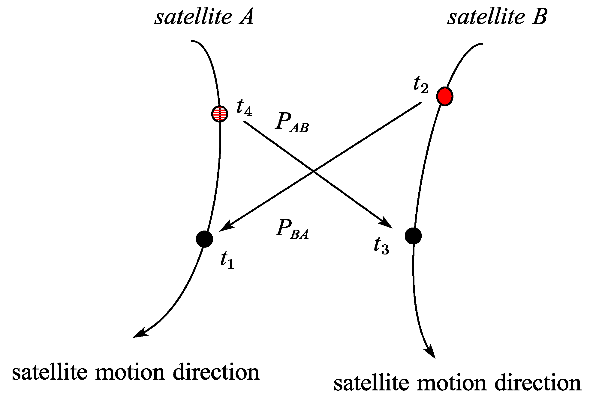
As shown in Figure 2, $t_1$, $t_2$, $t_3$, and $t_4$, respectively, represent the signal times for satellite A (LEO) reception, satellite B sending, satellite B reception, and satellite A sending. In practical applications, distance measurement can be performed based on the same signal transmission or reception time between two satellites. The assumption that follows is that the receiving time is the same, that is, $t_1=t_3$, and Reference [22] has proven that the non-strict equality between the two does not affect the accuracy of the calculation.

The dual one-way ranging process is as follows: Firstly, satellite A sends a ranging signal, and satellite B receives it at time $t_1$ on its clock face, obtaining the first one-way ranging signal $P_{\mathrm{A}\mathrm{B}}$. Then, satellite B emits a ranging signal, and satellite A receives it at time t₁ on its clock face, obtaining a second one-way ranging signal $P_{\mathrm{B}\mathrm{A}}$. Two measurement models with opposite directions are represented in a set of ranging values, which can be expressed as

$$\begin{array}{c}{P}_{\mathrm{A}\mathrm{B}}(t_1)=‖{\mathit{R}}_{\mathrm{B}}(t_1)-{\mathit{R}}_{\mathrm{A}}(t_1-{\tau }_{\mathrm{A}\mathrm{B}})‖+c·\delta {\tau }_{\mathrm{B}}(t_1)-c·\delta {\tau }_{\mathrm{A}}(t_1-{\tau }_{\mathrm{A}\mathrm{B}})+c·(D_{\mathrm{A}}^{\mathrm{s}\mathrm{d}}+D_{\mathrm{B}}^{\mathrm{r}\mathrm{e}})+{\epsilon }_{\mathrm{A}\mathrm{B}}\\ P_{\mathrm{B}\mathrm{A}}(t_1)=‖{\mathit{R}}_{\mathrm{A}}(t_1)-{\mathit{R}}_{\mathrm{B}}(t_1-{\tau }_{\mathrm{B}\mathrm{A}})‖+c·\delta {\tau }_{\mathrm{A}}(t_1)-c·\delta {\tau }_{\mathrm{B}}(t_1-{\tau }_{\mathrm{B}\mathrm{A}})+c·(D_{\mathrm{B}}^{\mathrm{s}\mathrm{d}}+D_{\mathrm{A}}^{\mathrm{r}\mathrm{e}})+{\epsilon }_{\mathrm{B}\mathrm{A}}\end{array}$$

(1)

In the equation, $c$ is the speed of light; $t_1=t_{\mathrm{A}}+\delta {\tau }_{\mathrm{A}}(t_{\mathrm{A}})=t_{\mathrm{B}}+\delta {\tau }_{\mathrm{B}}(t_{\mathrm{B}})$; ${\mathit{R}}_{\mathrm{A}}$ and ${\mathit{R}}_{\mathrm{B}}$ represent the position vectors of two satellites, respectively; and $\delta {\tau }_{\mathrm{A}}$ and $\delta {\tau }_{\mathrm{B}}$ are the clock offset of the satellites. $D_{\mathrm{A}}^{\mathrm{s}\mathrm{d}}$ and $D_{\mathrm{A}}^{\mathrm{r}\mathrm{e}}$ are the inter-satellite link payload sending and reception delays of satellite A, respectively; $D_{\mathrm{B}}^{\mathrm{s}\mathrm{d}}$ and $D_{\mathrm{B}}^{\mathrm{r}\mathrm{e}}$ represent the inter-satellite link payload sending and reception delays of satellite B, respectively; the equipment delays are related to temperature and change slowly, so these can be regarded as constants; ${\tau }_{\mathrm{A}\mathrm{B}}$ and ${\tau }_{\mathrm{B}\mathrm{A}}$ are signal propagation times; and ${\epsilon }_{\mathrm{A}\mathrm{B}}$ and ${\epsilon }_{\mathrm{B}\mathrm{A}}$ are measurement noise modeled as Gaussian white noise, with the calculation method described in Reference [23].

Combine the DOR values to obtain the double value of the distance [24]; that is,

$$\begin{array}{ll}{z}_{\mathrm{s}\mathrm{u}\mathrm{m}}(t_1)& ={\displaystyle \frac{1}{2}}[P_{\mathrm{A}\mathrm{B}}(t_1)+P_{\mathrm{B}\mathrm{A}}(t_1)]\\ & ={\displaystyle \frac{1}{2}}\left\{‖{\mathit{R}}_{\mathrm{B}}(t_1)-{\mathit{R}}_{\mathrm{A}}(t_1-{\tau }_{\mathrm{A}\mathrm{B}})‖+‖{\mathit{R}}_{\mathrm{A}}(t_1)-{\mathit{R}}_{\mathrm{B}}(t_1-{\tau }_{\mathrm{B}\mathrm{A}})‖+[c·(\delta {\tau }_{\mathrm{A}}(t_1)+\delta {\tau }_{\mathrm{B}}(t_1))]\right\}+\\ & {\displaystyle \frac{1}{2}}\left\{c·(D_{\mathrm{A}}^{\mathrm{s}\mathrm{d}}+D_{\mathrm{B}}^{\mathrm{r}\mathrm{e}}+D_{\mathrm{B}}^{\mathrm{s}\mathrm{d}}+D_{\mathrm{A}}^{\mathrm{r}\mathrm{e}})-[c·(\delta {\tau }_{\mathrm{A}}(t_1-{\tau }_{\mathrm{A}\mathrm{B}})+\delta {\tau }_{\mathrm{B}}(t_1-{\tau }_{\mathrm{B}\mathrm{A}}))]+({\epsilon }_{\mathrm{A}\mathrm{B}}+{\epsilon }_{\mathrm{B}\mathrm{A}})\right\}\\ & ={\displaystyle \frac{1}{2}}[{\mathrm{\rho }}_{\mathrm{A}\mathrm{B}}(t_1)+{\mathrm{\rho }}_{\mathrm{B}\mathrm{A}}(t_1)+c{D}_{\mathrm{s}\mathrm{u}\mathrm{m}}+{\epsilon }_{\mathrm{A}\mathrm{B}}+{\epsilon }_{\mathrm{B}\mathrm{A}}+c\mathrm{\Delta }\delta {\tau }_{\mathrm{B}}(t_1)+c\mathrm{\Delta }\delta {\tau }_{\mathrm{A}}(t_1)]\end{array}$$

(2)

In the equation, ${\mathrm{\rho }}_{\mathrm{A}\mathrm{B}}(t_1)=‖{\mathit{R}}_{\mathrm{B}}(t_1)-{\mathit{R}}_{\mathrm{A}}(t_1-{\tau }_{\mathrm{A}\mathrm{B}})‖$, and ${\mathrm{\rho }}_{\mathrm{B}\mathrm{A}}(t_1)=‖{\mathit{R}}_{\mathrm{A}}(t_1)-{\mathit{R}}_{\mathrm{B}}(t_1-{\tau }_{\mathrm{B}\mathrm{A}})‖$; $D_{\mathrm{s}\mathrm{u}\mathrm{m}}$ is the device latency of summing combination. $\mathrm{\Delta }\delta {\tau }_{\mathrm{A}}(t_1)$ and $\mathrm{\Delta }\delta {\tau }_{\mathrm{B}}(t_1)$ are the clock offset variation values during the measurement process. It can be seen that the above equation still includes the clock parameters of the satellite, and clock offset will have an impact on the calculated values of the equation. However, when the clock offset is small, this impact is much smaller than the satellite orbit error and can be disregarded.

The purpose of subtraction combination is to preserve the clock term and achieve the decoupling of the distance. However, due to the time of flight, the satellite will experience displacement during this process, resulting in differences in the geometric distances contained in the two pseudoranges, making it impossible to directly eliminate these differences. During the orbit determination process, the geometric distance correction term can be calculated through numerical integration of the orbit, and then the subtraction combination can be corrected. The expression is

$$\begin{array}{ll}{z}_{\mathrm{s}\mathrm{u}\mathrm{b}}(t_1)& ={\displaystyle \frac{1}{2}}[P_{\mathrm{A}\mathrm{B}}(t_1)+P_{\mathrm{B}\mathrm{A}}(t_1)]\\ & ={\displaystyle \frac{1}{2}}\left\{‖{\mathit{R}}_{\mathrm{B}}(t_1)-{\mathit{R}}_{\mathrm{A}}(t_1-{\tau }_{\mathrm{A}\mathrm{B}})‖+‖{\mathit{R}}_{\mathrm{A}}(t_1)-{\mathit{R}}_{\mathrm{B}}(t_1-{\tau }_{\mathrm{B}\mathrm{A}})‖+[c·(\delta {\tau }_{\mathrm{A}}(t_1)+\delta {\tau }_{\mathrm{B}}(t_1))]\right\}+\\ & {\displaystyle \frac{1}{2}}\left\{c·(D_{\mathrm{A}}^{\mathrm{s}\mathrm{d}}+D_{\mathrm{B}}^{\mathrm{r}\mathrm{e}}+D_{\mathrm{B}}^{\mathrm{s}\mathrm{d}}+D_{\mathrm{A}}^{\mathrm{r}\mathrm{e}})-[c·(\delta {\tau }_{\mathrm{A}}(t_1-{\tau }_{\mathrm{A}\mathrm{B}})+\delta {\tau }_{\mathrm{B}}(t_1-{\tau }_{\mathrm{B}\mathrm{A}}))]+({\epsilon }_{\mathrm{A}\mathrm{B}}+{\epsilon }_{\mathrm{B}\mathrm{A}})\right\}\\ & ={\displaystyle \frac{1}{2}}\{\Delta \mathrm{\rho }+c{D}_{\mathrm{s}\mathrm{u}\mathrm{b}}+{\epsilon }_{\mathrm{A}\mathrm{B}}-{\epsilon }_{\mathrm{B}\mathrm{A}}+c[\delta {\tau }_{\mathrm{B}}(t_1)+\delta {\tau }_{\mathrm{B}}(t_1-{\tau }_{\mathrm{B}\mathrm{A}})]-c[\delta {\tau }_{\mathrm{A}}(t_1)+\delta {\tau }_{\mathrm{A}}(t_1-{\tau }_{\mathrm{A}\mathrm{B}})]\end{array}$$

(3)

In the equation, $\mathrm{\Delta }\mathrm{\rho }$ is the geometric distance correction term; $D_{\mathrm{s}\mathrm{u}\mathrm{b}}$ is the total device latency. The above equation is still influenced by the satellite orbit, which can affect the calculated value of $\mathrm{\Delta }\mathrm{\rho }$. In the initial stage of orbit determination, the error in orbit estimation is relatively large; that is, $\mathrm{\Delta }\mathrm{\rho }$ is large. However, as the orbit determination results converge, the calculation error of this term tends to zero, and the residual error is negligible relative to the measurement noise of the inter-satellite link itself. If the LEO satellite clock is selected as the reference time system, then $\delta {\tau }_{\mathrm{A}}(t_1)$ and $\delta {\tau }_{\mathrm{A}}(t_1-{\tau }_{\mathrm{A}\mathrm{B}})$ are equal to 0.

3. Dynamic Model and Algorithms for Space-Based Orbit Determination

This section describes the orbital dynamic model and orbit determination algorithms for satellite navigation. In addition to introducing the commonly used sequential processing algorithm EKF, this section innovatively proposes non-overlapping and overlapping SWBP algorithms and makes detailed derivations.

3.1. Orbital Dynamic Model

Let $\mathit{Y}(t)={\left[\mathit{r}(t),\mathit{v}(t)\right]}^{\mathrm{T}}$ be the state vector of the satellite at time $t$. Through numerical integration of differential equations, satellite orbits can be extrapolated. The first-order ordinary differential equation of orbital dynamics is [25]

$$\left\{\begin{array}{l}\begin{array}{l}{\displaystyle \frac{\mathrm{d}\mathit{r}}{\mathrm{d}t}}=\mathit{v}\hfill \\ {\displaystyle \frac{\mathrm{d}\mathit{v}}{\mathrm{d}t}}={\mathit{a}}_{\mathrm{e}}+{\mathit{a}}_{\mathrm{m}}+{\mathit{a}}_{\mathrm{s}}+{\mathit{a}}_{\mathrm{s}\mathrm{p}}+{\mathit{a}}_{\mathrm{N}\mathrm{B}}+{\mathit{a}}_{\mathrm{d}\mathrm{r}\mathrm{g}}+\mathit{u}\hfill \end{array}\hfill \end{array}\right.$$

(4)

In the equation, $\mathit{r}$ and $\mathit{v}$ are the position and velocity vectors of the satellites, respectively; ${\mathit{a}}_{\mathrm{e}}$, ${\mathit{a}}_{\mathrm{m}}$, and ${\mathit{a}}_{\mathrm{s}}$ represent the gravitational acceleration of the Earth, Moon, and Sun, respectively; ${\mathit{a}}_{\mathrm{s}\mathrm{p}}$ is the acceleration of solar pressure; ${\mathit{a}}_{\mathrm{N}\mathrm{B}}$ is the gravitational perturbation acceleration of N-body; ${\mathit{a}}_{\mathrm{d}\mathrm{r}\mathrm{g}}$ is the atmospheric resistance acceleration; and u is the process noise used to compensate for dynamic model errors. The differential equation of state can be simplified and expressed as

$${\displaystyle \frac{\mathrm{d}\mathit{Y}(t)}{\mathrm{d}t}}=g(\mathit{Y}(t),\mathit{u},t)=\left(\begin{array}{c}\mathit{v}\\ \mathit{a}\end{array}\right)$$

(5)

At the initial epoch, the orbit state of the satellite is $\mathit{Y}(t_0)$, so the state transition matrix from $t_0$ to $t$ is [26]

$${\mathit{\Phi }}_{t\left|t_0\right.}={\displaystyle \frac{\mathsf{\partial }\mathit{Y}(t)}{\mathsf{\partial }\mathit{Y}(t_0)}}$$

(6)

The transition matrix from noise to state during the acceleration process is ${\mathit{\Gamma }}_u$, represented as

$${\mathit{\Gamma }}_u={\displaystyle \frac{\mathsf{\partial }\mathit{Y}(t)}{\mathsf{\partial }\mathit{u}(t_0)}}=\left[\begin{array}{c}{\displaystyle \frac{\mathrm{\Delta }{t}^2}{2}}\times {\mathit{I}}_{3\times 3}\\ \mathrm{\Delta }t\times {\mathit{I}}_{3\times 3}\end{array}\right]$$

(7)

where $\mathit{I}$ is the identity matrix; $\mathrm{\Delta }t$ is the integration step size.

The partial derivative of the dynamic parameter p with respect to $\mathit{Y}(t)$ is a sensitive matrix, denoted as

$$\mathit{S}(t)={\displaystyle \frac{\mathsf{\partial }\mathit{Y}(t)}{\mathsf{\partial }p}}$$

(8)

In the equation, $p=[C_{\mathrm{r}}]$; $C_{\mathrm{r}}$ is the solar radiation pressure coefficient.

The partial derivative of the sensitive matrix is

$${\displaystyle \frac{\mathrm{d}\mathit{S}(t)}{\mathrm{d}t}}=\left(\begin{array}{cc}{0}_{3\times 3}& {\mathit{I}}_{3\times 3}\\ {\displaystyle \frac{\mathsf{\partial }\mathit{a}(t,r,v,p)}{\mathsf{\partial }\mathit{r}(t)}}& {\displaystyle \frac{\mathsf{\partial }\mathit{a}(t,r,v,p)}{\mathsf{\partial }\mathit{v}(t)}}\end{array}\right)·\mathit{S}(t)+\left(\begin{array}{c}0\\ {\displaystyle \frac{\mathsf{\partial }\mathit{a}(t,r,v,p)}{\mathsf{\partial }p}}\end{array}\right)$$

(9)

The variational equation obtained by combining the state transition matrix and the sensitivity matrix is

$${\displaystyle \frac{\mathrm{d}(\mathit{\Phi },\mathit{S})}{\mathrm{d}t}}=\left(\begin{array}{cc}0& I\\ {\displaystyle \frac{\mathsf{\partial }\mathit{a}}{\mathsf{\partial }\mathit{r}}}& {\displaystyle \frac{\mathsf{\partial }\mathit{a}}{\mathsf{\partial }\mathit{v}}}\end{array}\right)·(\mathit{\Phi },\mathit{S})+\left(\begin{array}{cc}0& 0\\ 0& {\displaystyle \frac{\mathsf{\partial }\mathit{a}}{\mathsf{\partial }p}}\end{array}\right)$$

(10)

Equations (5) and (10) are the equations required for orbit extrapolation. After integration, new state transition matrices and sensitivity matrices can be obtained, providing new satellite state information.

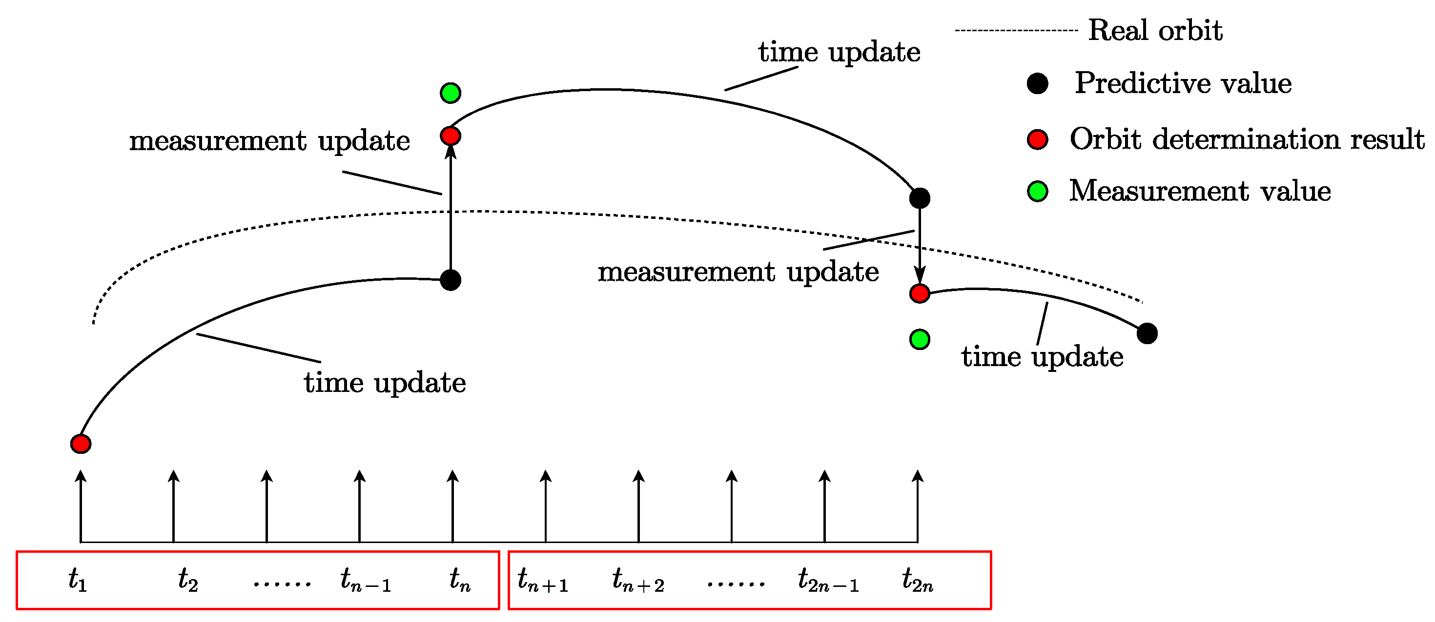
3.2. Extended Kalman Filter Algorithm

The Extended Kalman Filter is easy to implement and commonly used for real-time orbit determination [27]. The estimated state quantity is defined as

$$\mathit{X}={({\mathit{r}}^{\mathrm{T}},{\mathit{v}}^{\mathrm{T}},C_{\mathrm{r}},c{D}_{\mathrm{s}\mathrm{u}\mathrm{m}})}^{\mathrm{T}}$$

(11)

In the equation, $c$ is the speed of light; $D_{\mathrm{s}\mathrm{u}\mathrm{m}}$ is the device delay for summing up combinations. EKF orbit determination has two steps: the ‘time update’ step calculates the predicted state for the next epoch by integrating the state of the previous epoch; and the ‘measurement update’ uses the current epoch measurement data to correct the predicted state of the ‘time update’, with the filtering process shown in Figure 3.

A nonlinear system can be modeled as

$$\left\{\begin{array}{l}{\mathit{X}}_{k+1}=f({\mathit{X}}_k)+{\mathit{\Gamma }}_u{\mathit{u}}_k\hfill \\ {\mathit{Z}}_{k+1}=h({\mathit{X}}_{k+1})+{\mathit{v}}_{k+1}\hfill \end{array}\right.$$

(12)

In the equation, ${\mathit{Z}}_{k+1}$ is the measurement vector; $f(·)$ and $h(·)$ are the nonlinear state function and measurement function of the system, respectively; and ${\mathit{u}}_k$ and ${\mathit{v}}_k$ are uncorrelated noise with a covariance of ${\mathit{Q}}_k$ and ${\mathit{R}}_k$, respectively.

At time $t_{k+1}$, the process of the ‘time update’ is represented as

$$\left\{\begin{array}{l}{\mathit{X}}_{k+1}^{-}=\mathit{X}[t_{k+1},\mathit{X}(t_k)=X_k^{+}]\hfill \\ {\mathit{P}}_{k+1}^{-}={\Phi }_{k+1\left|k\right.}{\mathit{P}}_k^{+}{\Phi }_{k+1\left|k\right.}^{\mathrm{T}}+{\mathit{\Gamma }}_{k+1\left|k\right.}^u{\mathit{Q}}_k{({\mathit{\Gamma }}_{k+1\left|k\right.}^u)}^{\mathrm{T}}\hfill \end{array}\right.$$

(13)

In the equation,

$${\mathit{\Gamma }}_{k+1\left|k\right.}^u=\left[\begin{array}{c}{\mathit{\Gamma }}_u(t_{k+1})\\ {\mathbf{0}}_{2\times 3}\end{array}\right]$$

(14)

The bidirectional observation value of epoch $t_{k+1}$ is

$${\mathit{Z}}_{k+1}=\left[\begin{array}{c}{Z}_{\mathrm{s}\mathrm{u}\mathrm{m}}(t_{k+1})\\ Z_{\mathrm{s}\mathrm{u}\mathrm{b}}(t_{k+1})\end{array}\right]$$

(15)

The design matrix can be represented as

$${\mathit{H}}_{k+1}=\left[\begin{array}{c}{\displaystyle \frac{\mathsf{\partial }{Z}_{\mathrm{s}\mathrm{u}\mathrm{m}}(t_{k+1})}{\mathsf{\partial }{\mathit{X}}_{k+1}^{-}}}\\ {\displaystyle \frac{\mathsf{\partial }{Z}_{\mathrm{s}\mathrm{u}\mathrm{b}}(t_{k\mathsf{\varpi }1})}{\mathsf{\partial }{\mathit{X}}_{k+1}^{-}}}\end{array}\right]$$

(16)

‘Measurement update’ uses the measurement data at that moment to correct the prior state ${\mathit{X}}_{k+1}^{-}$ and the prior covariance matrix ${\mathit{P}}_{k+1}^{-}$. The calculation process is as follows:

$$\left\{\begin{array}{l}{\mathit{K}}_{k+1}={\mathit{P}}_{k+1}^{-}{\mathit{H}}_{k+1}^{\mathrm{T}}{({\mathit{R}}_{k+1}+{\mathit{H}}_{k+1}{\mathit{P}}_{k+1}^{-}{\mathit{H}}_{k+1}^{\mathrm{T}})}^{-1}\hfill \\ {\mathit{X}}_{k+1}^{+}={\mathit{X}}_{k+1}^{-}+{\mathit{K}}_{k+1}[{\mathit{Z}}_{k+1}-h({\mathit{X}}_{k+1}^{-})]\hfill \\ {\mathit{P}}_{k+1}^{+}=(\mathit{I}-{\mathit{K}}_{k+1}{\mathit{H}}_{k+1}){\mathit{P}}_{k+1}^{-}{(\mathit{I}-{\mathit{K}}_{k+1}{\mathit{H}}_{k+1})}^{\mathrm{T}}+{\mathit{K}}_{k+1}{\mathit{R}}_{k+1}{\mathit{K}}_{k+1}^{\mathrm{T}}\hfill \end{array}\right.$$

(17)

In the equation, ${\mathit{K}}_{k+1}$ is the Kalman filter gain; $\mathit{I}$ is the identity matrix; and ${\mathit{X}}_{k+1}^{+}$ and ${\mathit{P}}_{k+1}^{+}$ represent the posterior state and covariance after the measurement update. ${\mathit{P}}_{k+1}^{+}$ can be used to evaluate the accuracy of the filtered state.

3.3. Non-Overlapping Sliding-Window Batch Processing Algorithm

The aforementioned EKF is used to process the nonlinear system to obtain an approximate linearized model, which has real-time performance, but the accuracy is not enough for the case of strong nonlinearity, and the selection of the initial value has certain requirements.

Correspondingly, the core idea of batch processing is to accumulate a batch of data first and then carry out optimization processing according to this batch of data. This method is more complicated and lacks real-time computation.

The orbit determination algorithm in this paper combines the ideas of the above two algorithms at the same time, using multiple historical epoch measurements and current epoch measurements to update the estimated state of the current epoch orbit. Although the form is similar to the sequential processing algorithm, it incorporates the accumulation of historical data in the updating process, which is expected to improve the stability and accuracy of orbit determination under large initial errors on the basis of the EKF.

When the step size of the sliding window is equal to the length of the time window, this paper defines it as the non-overlapping Sliding-Window Batch Processing algorithm, which is also a special Sliding-Window Batch Processing orbit determination algorithm.

The non-overlapping Sliding-Window Batch Processing algorithm has two steps: the ‘time update’ step is the same as the EKF step, and the ‘measurement update’ is conducted to correct the predicted state of the ‘time update’ using measurement data from previous epochs at a specific epoch. The orbit determination process is shown in Figure 4. When the capacity of the window is n epochs, only the last epochs $t_n$, $t_{2n}$, etc., of this batch are updated by measurement. The first n−1 epochs in each window are only extrapolated through time updates.

Take the first window as an example; that is, ${\mathit{X}}_i^{+}={\mathit{X}}_i^{-}(i=1,2\cdots n-1)$. After completing the time update step, the epochs ${\mathit{X}}_i^{-}$ are known, satisfying the following relationship:

$${\mathit{X}}_{i+1}^{-}={\mathit{\Phi }}_{i+1\left|i\right.}·{\mathit{X}}_i^{-}$$

(18)

These values are accompanied by the inter-satellite link measurement values $Z_i^{\mathrm{s}\mathrm{u}\mathrm{m}}$ and $Z_i^{\mathrm{s}\mathrm{u}\mathrm{b}}$. The design matrix of the Sliding-Window Batch Processing algorithm is

$${\mathit{H}}_{\mathrm{B}}={\left[\begin{array}{ccccccc}{\displaystyle \frac{\mathsf{\partial }{Z}_1^{\mathrm{s}\mathrm{u}\mathrm{m}}}{\mathsf{\partial }{\mathit{X}}_n^{-}}}& {\displaystyle \frac{\mathsf{\partial }{Z}_1^{\mathrm{s}\mathrm{u}\mathrm{b}}}{\mathsf{\partial }{\mathit{X}}_n^{-}}}& {\displaystyle \frac{\mathsf{\partial }{Z}_2^{\mathrm{s}\mathrm{u}\mathrm{m}}}{\mathsf{\partial }{\mathit{X}}_n^{-}}}& {\displaystyle \frac{\mathsf{\partial }{Z}_2^{\mathrm{s}\mathrm{u}\mathrm{b}}}{\mathsf{\partial }{\mathit{X}}_n^{-}}}& \cdots & {\displaystyle \frac{\mathsf{\partial }{Z}_n^{\mathrm{s}\mathrm{u}\mathrm{m}}}{\mathsf{\partial }{\mathit{X}}_n^{-}}}& {\displaystyle \frac{\mathsf{\partial }{Z}_n^{\mathrm{s}\mathrm{u}\mathrm{b}}}{\mathsf{\partial }{\mathit{X}}_n^{-}}}\end{array}\right]}^{\mathrm{T}}$$

(19)

In the equation, the calculated values are

$$\left\{\begin{array}{c}{\displaystyle \frac{\mathsf{\partial }{Z}_i^{\mathrm{s}\mathrm{u}\mathrm{m}}}{\mathsf{\partial }{\mathit{X}}_n^{-}}}={\mathit{H}}_i^{\mathrm{s}\mathrm{u}\mathrm{m}}{\mathit{\Phi }}_{i\left|n\right.}\\ {\displaystyle \frac{\mathsf{\partial }{Z}_i^{\mathrm{s}\mathrm{u}\mathrm{b}}}{\mathsf{\partial }{\mathit{X}}_n^{-}}}={\mathit{H}}_i^{\mathrm{s}\mathrm{u}\mathrm{b}}{\mathit{\Phi }}_{i\left|n\right.}\end{array}\right.$$

(20)

where $i=1,2\cdots n$, and ${\mathit{\Phi }}_{i\left|n\right.}$ is the state transition matrix from the n epoch to the i epoch through reverse integration.

The Kalman filter gain is

$$\mathit{K}={\displaystyle \frac{{\mathit{P}}_n^{-}{\mathit{H}}_{\mathrm{B}}^{\mathrm{T}}}{{\mathit{H}}_{\mathrm{B}}{\mathit{P}}_n^{-}{\mathit{H}}_{\mathrm{B}}^{\mathrm{T}}+\mathit{R}}}$$

(21)

In the equation, ${\mathit{P}}_n^{-}$ represents the prior covariance of the state at the time $t_n$ when it is necessary to measure and update the epoch; $\mathit{R}$ is the measurement noise matrix.

When reaching the epoch that requires a measurement update, the inter-satellite measurement data vector and measurement model calculation value vector for this batch of epochs can already be obtained:

$$\begin{array}{l}{\mathit{Z}}_{\mathrm{o}\mathrm{b}}={\left[\begin{array}{ccccccc}{Z}_1^{\mathrm{s}\mathrm{u}\mathrm{m}}& Z_1^{\mathrm{s}\mathrm{u}\mathrm{b}}& Z_2^{\mathrm{s}\mathrm{u}\mathrm{m}}& Z_2^{\mathrm{s}\mathrm{u}\mathrm{b}}& \cdots & Z_n^{\mathrm{s}\mathrm{u}\mathrm{m}}& Z_n^{\mathrm{s}\mathrm{u}\mathrm{b}}\end{array}\right]}^{\mathrm{T}}\\ \widehat{\mathit{Z}}={\left[\begin{array}{ccccccc}{\widehat{Z}}_1^{\mathrm{s}\mathrm{u}\mathrm{m}}& {\widehat{Z}}_1^{\mathrm{s}\mathrm{u}\mathrm{b}}& {\widehat{Z}}_2^{\mathrm{s}\mathrm{u}\mathrm{m}}& {\widehat{Z}}_2^{\mathrm{s}\mathrm{u}\mathrm{b}}& \cdots & {\widehat{Z}}_n^{\mathrm{s}\mathrm{u}\mathrm{m}}& {\widehat{Z}}_n^{\mathrm{s}\mathrm{u}\mathrm{b}}\end{array}\right]}^{\mathrm{T}}\end{array}$$

(22)

Therefore, the estimated state value at time $t_n$ is

$${\mathit{X}}_n^{+}={\mathit{X}}_n^{-}+\mathit{K}·({\mathit{Z}}_{\mathrm{o}\mathrm{b}}-\widehat{\mathit{Z}})$$

(23)

The covariance matrix of state estimation error is

$${\mathit{P}}_n^{+}=(\mathit{I}-\mathit{K}{\mathit{H}}_{\mathrm{B}}){\mathit{P}}_n^{-}{(\mathit{I}-\mathit{K}{\mathit{H}}_{\mathrm{B}})}^{\mathrm{T}}+\mathit{K}\mathit{R}{\mathit{K}}^{\mathrm{T}}$$

(24)

where $\mathit{I}$ is the identity matrix.

3.4. Overlapping Sliding-Window Batch Processing Algorithm

Non-overlapping Sliding-Window Batch Processing somewhat reduces the frequency of measurement updates. When the step size of the sliding window is less than the length of the time window, this paper defines it as the overlapping Sliding-Window Batch Processing algorithm. This algorithm can maintain the frequency of measurement updates and has the potential to use better design matrix data for updates. Assuming that the capacity of a window is still n epochs (n ≥ 4), whether overlapping or non-overlapping, measurement updates are only performed on the last epoch in the window. The difference is that in non-overlapping situations, the first n − 1 epochs in a window have only undergone time update extrapolation; in overlapping situations, some of the first n − 1 epochs in a window have already undergone the measurement update processing of the previous batch of data, so there may be a situation of orbit discontinuity in the current window. To avoid this discontinuity, it is necessary to start from the measurement-updated epoch and perform reverse integration to update the state values of the first few epochs in the window. In theory, the updated state is closer to the real orbit, and using the updated data for measurement updates can achieve better filtering effects. Figure 5 is a schematic figure of orbit determination with a window capacity of four epochs, sliding forward two epochs at a time. In this figure, $t_4$, $t_6$, $t_8$, $t_{10}$, etc., are the measurement update epochs, while $t_3$, $t_5$, $t_7$, etc., are the reverse integration epochs.

The step size of each window sliding is two epochs; that is, the n − 2 epoch in the current window is the measurement updated epoch of the previous batch window. Then, the historical data will be updated in this window for the first to n − 3 historical epochs through reverse integration. Compared with non-overlapping Sliding-Window Batch Processing, some design matrices and state transition matrices in the equation will change after reverse integration.

$$\left\{\begin{array}{c}{\displaystyle \frac{\mathsf{\partial }{Z}_i^{\mathrm{s}\mathrm{u}\mathrm{m}}}{\mathsf{\partial }{\mathit{X}}_n^{-}}}={\displaystyle \frac{\mathsf{\partial }{Z}_i^{\mathrm{s}\mathrm{u}\mathrm{m}}}{\mathsf{\partial }{\mathit{X}}_i^{\ast }}}{\displaystyle \frac{\mathsf{\partial }{\mathit{X}}_i^{\ast }}{\mathsf{\partial }{\mathit{X}}_{i+1}^{\ast }}}\cdots {\displaystyle \frac{\mathsf{\partial }{\mathit{X}}_{n-2}^{+}}{\mathsf{\partial }{\mathit{X}}_{n-1}^{-}}}{\displaystyle \frac{\mathsf{\partial }{\mathit{X}}_{n-1}^{-}}{\mathsf{\partial }{\mathit{X}}_n^{-}}}={\widehat{\mathit{H}}}_i^{\mathrm{s}\mathrm{u}\mathrm{m}}{\mathit{\Phi }}_{i\left|n\right.}\\ {\displaystyle \frac{\mathsf{\partial }{Z}_i^{\mathrm{s}\mathrm{u}\mathrm{b}}}{\mathsf{\partial }{\mathit{X}}_n^{-}}}={\displaystyle \frac{\mathsf{\partial }{Z}_i^{\mathrm{s}\mathrm{u}\mathrm{b}}}{\mathsf{\partial }{\mathit{X}}_i^{\ast }}}{\displaystyle \frac{\mathsf{\partial }{\mathit{X}}_i^{\ast }}{\mathsf{\partial }{\mathit{X}}_{i+1}^{\ast }}}\cdots {\displaystyle \frac{\mathsf{\partial }{\mathit{X}}_{n-2}^{+}}{\mathsf{\partial }{\mathit{X}}_{n-1}^{-}}}{\displaystyle \frac{\mathsf{\partial }{\mathit{X}}_{n-1}^{-}}{\mathsf{\partial }{\mathit{X}}_n^{-}}}={\widehat{\mathit{H}}}_i^{\mathrm{s}\mathrm{u}\mathrm{b}}{\mathit{\Phi }}_{i\left|n\right.}\end{array}\right.$$

(25)

In the equation, $i=1,2\cdots n$; ${\mathit{X}}_k^{\ast }(k=1,2\cdots n-3)$ is the epoch updated in reverse; and ${\mathit{X}}_{n-2}^{+}$ is the epoch measurement updated in the previous window, and therefore, it is a posterior value. Due to the change in the state of epoch $t_k(k=1,2\cdots n-3)$ compared to in non-overlapping Sliding-Window Batch Processing, its corresponding design matrix has also been changed to ${\widehat{\mathit{H}}}_k^{\mathrm{s}\mathrm{u}\mathrm{m}}$ and ${\widehat{\mathit{H}}}_k^{\mathrm{s}\mathrm{u}\mathrm{b}}$$(k=1,2\cdots n-3)$. Replace the corresponding variable in the non-overlapping sliding-window batch with the updated variable; the remaining equations are the same as those in the non-overlapping Sliding-Window Batch Processing.

In this paper, the overlapping Sliding-Window Batch Processing algorithm has different window capacities, but the window movement step size is the same, that is, sliding forward two epochs each time.

4. Space-Based Orbit Determination Results

The simulation of the measurement process adopts the DOR model introduced in Section 2, and the measurement values are the code pseudorange obtained from the measurements in both directions between satellites. The core idea of this research is to combine the dynamic models of two satellites (LEO satellite and Earth–Moon satellite) and inter-satellite link measurement data, use the EKF and the Sliding-Window Batch Processing algorithm introduced in Section 3 to perform space-based orbit determination of satellites, and analyze the orbit determination effect of the algorithm.

The experiment of space-based orbit determination is divided into simulated data simulation and an onboard data test. In the simulation of simulated data, the Earth–Moon satellite is located in DRO. This section mainly examines the orbit determination performance of various algorithms under different LEO positioning errors and DRO initial errors.

In the test of onboard data, the satellite measurement data is the K-band link data between the DRO-A satellite in the transfer orbit and DRO-L satellite in the LEO of a pilot mission (the inter-satellite distance is about 660,000 km). Among them, the DRO-L satellite’s orbit is calculated by the GNSS, and the reference orbit of the DRO-A satellite is calculated by ground-based orbit determination. The measurement data is obtained through the true dual one-way pseudorange measurement between satellites. This subsection mainly verifies the effectiveness of the algorithm proposed in this paper.

4.1. Simulation Using Simulated Data

4.1.1. Simulation Settings

The LEO used in the simulation process is a Sun-synchronous orbit at an altitude of 500 km, with a period of 1.5 h, a semi-major axis of 6878 km, an orbital inclination of 97.4°, an ascending node right ascension of 10.4°, an eccentricity of 0, and both the argument of perigee and true anomaly at 0°. The pseudorange measurement process only uses the LEO satellite’s position, so its velocity error is not considered. The positioning error of the LEO satellite’s orbit can be divided into two types of situations during simulation data: 0.2 and 10 m. The 0.2 m error assumes that the LEO satellite is equipped with a dual-frequency receiver, using the carrier phase, which uses the combination of ionospheric elimination data for navigation; the 10 m error assumes that the LEO satellite is equipped with a single-frequency receiver, using code pseudorange data to achieve the positioning level.

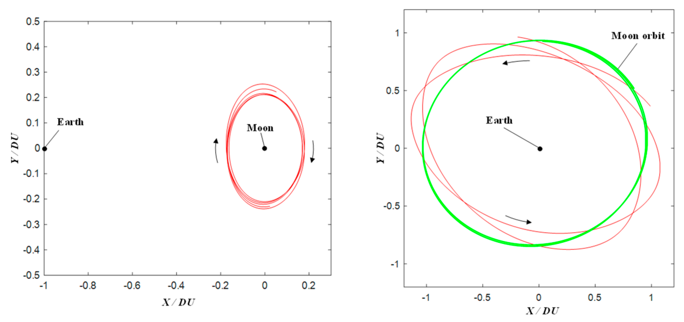
The satellite in DRO is located near the Moon, and its direction of motion around the Moon is opposite to the direction of the Earth’s revolution in the Earth–Moon rotation system, while its direction of rotation around the Earth in the geocentric inertial system is the same as the direction of the Moon’s revolution. The period of the Moon’s revolution is an integer ratio to the period of the satellite’s motion around the Moon in that orbit, which is called the resonance ratio [28]. As shown in the Figure 6, this section of the simulation uses DRO with a resonance ratio of 2:1, where DU refers to the average distance between the Earth and the Moon.

The simulation considers the issue of inter-satellite links being obstructed by the Earth and Moon. Except for the interruption of the link caused by the obstruction of the Earth and Moon, there are continuous measurement data at all other times, with a measurement step of 60 s and approximately 800 sets of measurement data per day.

4.1.2. Analysis of the Impact of the LEO Satellite’s Positioning Error

Simulation Result

This section of simulation mainly studies the orbit determination effects of the EKF and Sliding-Window Batch Processing algorithm under different LEO positioning errors and DRO initial state error conditions. The Sliding-Window Batch Processing algorithm with a window capacity of n, whether overlapping or non-overlapping, is simplified as ‘n epoch overlapping/non-overlapping SWBP’. In order to simplify the calculation, the position and velocity error parameters of LEO and DRO in each direction of the orthogonal coordinate system are the same, and the standard deviation of the ranging error is set to 1 m. The orbit determination parameters for the simulation process are set as shown in

Table 1. Parameter settings for orbit determination simulation in LEO positioning error impact analysis.

Parameter	Value
DRO initial position error/km	$100/500 (1-\sigma$)
DRO initial velocity error/(m/s)	$1/5 (1-\sigma$)
LEO positioning error/m	0.2/10
initial solar pressure coefficient error	0.2
standard deviation of distance measurement error/m	1
process noise (R/T/N)/(m/s2)	1 × 10−13/1 × 10−13/1 × 10−13

.

DRO’s orbit determination results are compared with its reference orbit (true value) to calculate the residuals, which are used to indicate the error level of the orbit determination results. As shown in

Table 2. DRO dynamic model and integrator for analyzing the impact of LEO positioning errors.

Parameter	Reference Orbit	Setting of Orbit Determination
the gravitational field of the Earth	12 × 12EGM2008	1 × 1GGM01C
the gravitational field of the Moon	20 × 20GRAIL660	1 × 1GRAIL660
the gravitational field of the Sun	particle model	particle model
Integrator	RKF78	RK4
integral step size/s	60	60

, in the simulation, the reference orbit simulates the real orbit, using a high-order dynamic model and integrator. The orbit determination uses a dynamic model that differs from the ‘real physical orbit’, and a lower-order gravitational field and integrator can be used.

The orbit determination results for DRO with an initial position error of 100 km and an initial velocity error of 1 m/s under different positioning error conditions of the LEO satellite are shown in Figure 7 and Figure 8. In the figures, the n-epoch non-overlapping Sliding-Window Batch Processing algorithm is referred to as ‘n epochs, non-overlapping’, and the n-epoch overlapping Sliding-Window Batch Processing algorithm is referred to as ‘n epochs, overlapping’. To quantify the convergence speed, it is established that the convergence standard is reached when the orbital residual reaches 100 m or less. To evaluate the accuracy of orbit determination, the root mean square of the last 20% of the orbit determination results is calculated as the indicator of orbit determination accuracy. The simulation results show the following:

(1)

Under the two initial conditions, the convergence accuracy of the EKF is 64.29 m and 592.02 m, respectively, and the convergence time is 227.04 h and 680.18 h, respectively.

(2)

When the LEO satellite’s positioning error is 0.2 m, the SWBP algorithm does not show significant improvement in orbit determination performance compared to the EKF. However, when the LEO satellite’s positioning error increases to 10 m, the SWBP algorithm, especially the 14-epoch overlapping SWBP, significantly improves the orbit determination accuracy, manifesting as the following:

①

Convergence speed: The 14-epoch overlapping SWBP algorithm can reach the convergence standard at 28.56 h, while the EKF can only reach the convergence standard at 680.18 h.

②

Convergence accuracy: The position accuracy of the 14-epoch overlapping SWBP algorithm is 25.85 m, while the EKF’s is only 592.02 m.

Through a comparison of the results, it can be seen that the orbit determination results of the DRO satellite under the EKF are more sensitive to changes in the positioning error of the LEO satellite, while the SWBP algorithm has good robustness and can maintain a fast convergence speed and accuracy in orbit determination even when the positioning error of the LEO satellite increases.

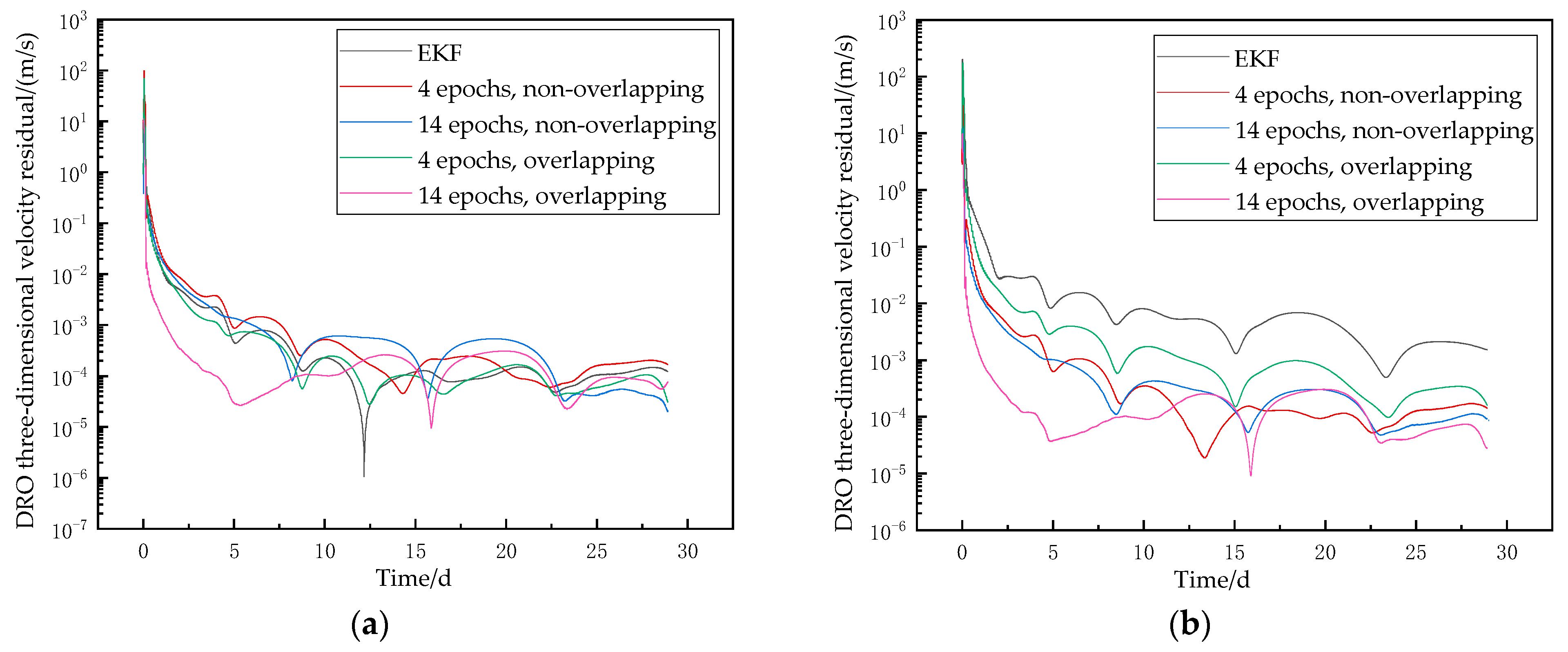
The velocity results for the above conditions are shown in Figure 9. As can be seen from the figure, the trend of the resultant line for velocity is roughly similar to that for position. When the LEO satellite’s positioning error is 0.2 m, a velocity accuracy of the order of 1 × 10⁻⁴ or better is achievable with all algorithms. When the LEO satellite’s positioning error increases to 10 m, the SWBP algorithm can achieve a velocity accuracy of 1 × 10⁻⁴ orders of magnitude and 1 × 10⁻⁵ orders of magnitude, but the EKF algorithm has a final accuracy of only 1.92 × 10⁻³ m/s.

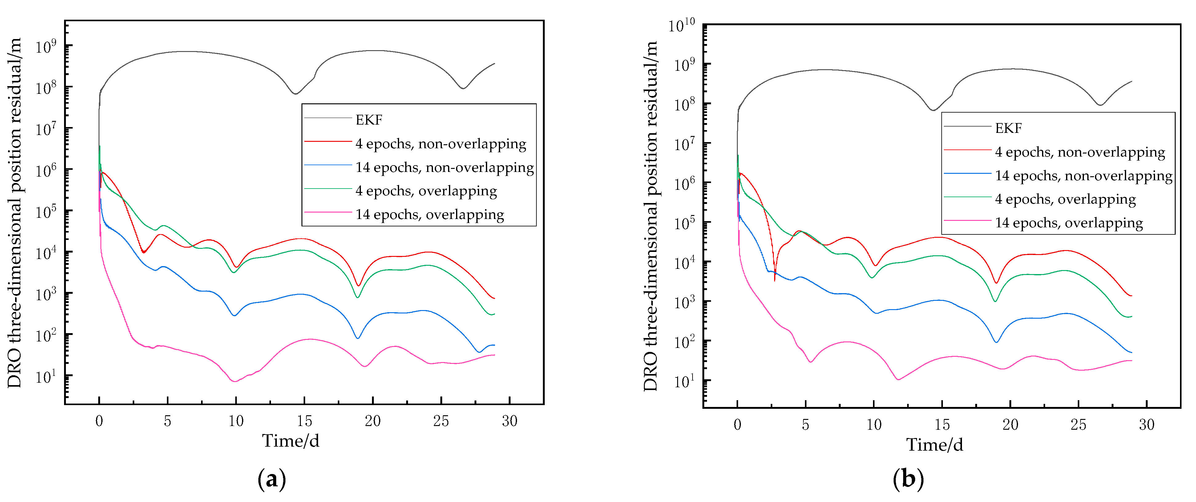
Increase the initial position error of the DRO satellite to 500 km and the initial velocity error to 5 m/s. The corresponding position results are shown in Figure 10. From the results, it can be seen that increased LEO satellite positioning error will have a negative impact on the results. When the initial state error of the DRO satellite’s orbit is too large, the EKF cannot achieve orbit determination convergence. Relatively speaking, the SWBP algorithm can still maintain the convergence trend of the orbit, and its orbit determination performance is relatively better when using a larger window capacity. When the window length of the SWBP algorithm is 14 epochs, the orbit determination accuracy can fall below 30 m.

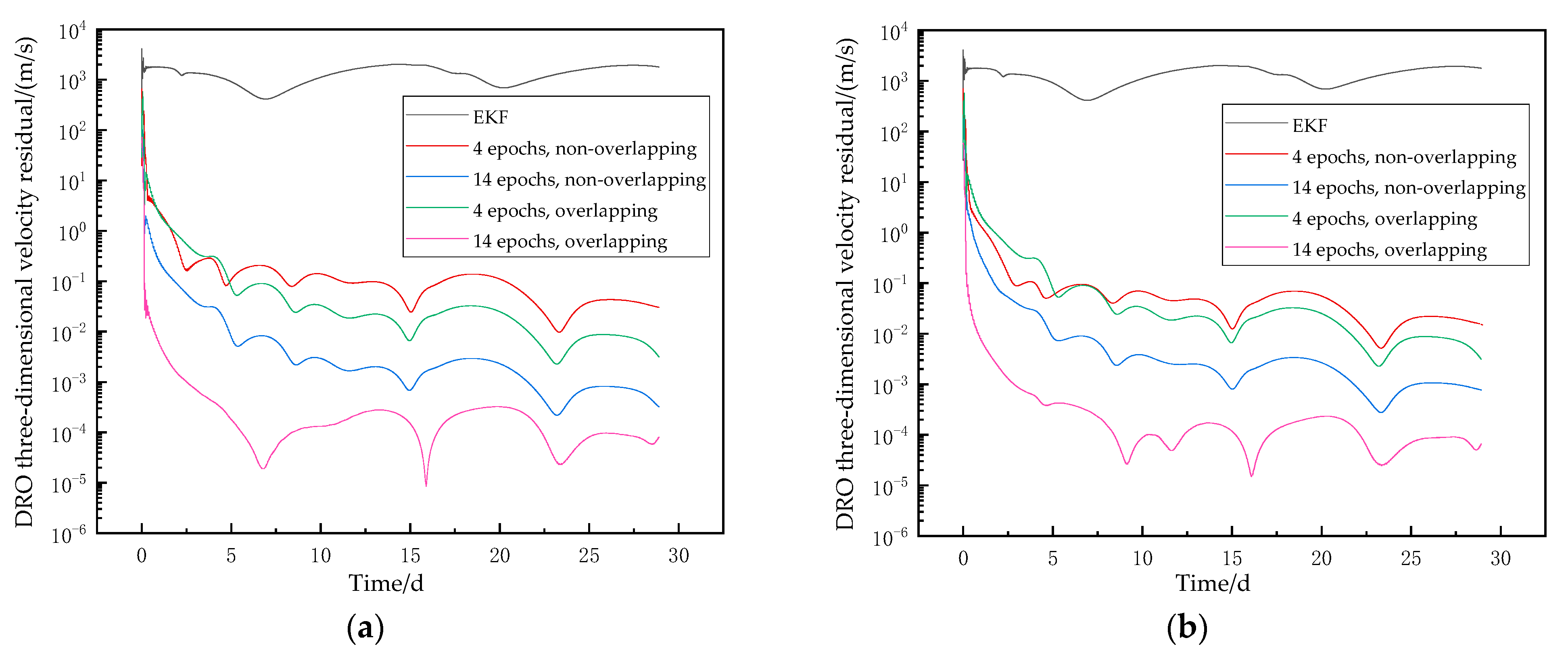
Correspondingly, the results of the orbit determination of velocity are shown in Figure 11. The velocity accuracy after using the SWBP algorithm is up to 0.1 m/s or even higher.

The results of the above orbit determination are summarized in

Table 3. Statistical results of DRO satellite orbit determination when DRO’s initial error is 100 km.

LEO Positioning Error/m		Root Mean Square of Residual 3D Position in Orbit Determination/m
	EKF	4 Epochs, Non-Overlapping	14 Epochs, Non-Overlapping	4 Epochs, Overlapping	14 Epochs, Overlapping
0.2	64.29	104.58	34.57	51.03	28.31
10.0	592.02	82.16	59.73	60.98	25.85
LEO Positioning Error/m		Time Taken to Reach Convergence Criteria/h
	EKF	4 Epochs, Non-Overlapping	14 Epochs, Non-Overlapping	4 Epochs, Overlapping	14 Epochs, Overlapping
0.2	227.04	242.55	82.27	116.12	35.32
10.0	680.20	390.68	257.04	242.55	28.62

and

Table 4. Statistical results of DRO satellite orbit determination when DRO’s initial error is 500 km.

LEO Positioning Error/m		Root Mean Square of Residual 3D Position in Orbit Determination/m
	EKF	4 Epochs, Non-Overlapping	14 Epochs, Non-Overlapping	4 Epochs, Overlapping	14 Epochs, Overlapping
0.2	\	2703.74	71.23	1089.04	23.79
10.0	\	5194.82	139.48	1280.95	23.92
LEO Positioning Error/m		Time Taken to Reach Convergence Criteria/h
	EKF	4 Epochs, Non-Overlapping	14 Epochs, Non-Overlapping	4 Epochs, Overlapping	14 Epochs, Overlapping
0.2	\	\	638.16	\	56.24
10.0	\	\	665.04	\	97.04

‘\’ implies that the convergence criterion has not been met.

. In the tables, the n-epoch overlapping/non-overlapping SWBP algorithms are referred to as ‘n epochs, overlapping/non-overlapping’.

Discussion and Analysis

From the above simulation results, it can be seen that

(1)

A decrease in the positioning accuracy of the LEO satellite will affect the orbit determination results of the DRO satellite. Orbit determination requires the use of the LEO satellite’s position, and a decrease in position accuracy is equivalent to an increase in measurement errors, resulting in a decrease in the convergence speed and accuracy of satellite orbit determination. Compared to the EKF, the orbit determination results of the SWBP algorithm are less affected by this error.

(2)

The larger the initial error of DRO, the more obvious the advantage of the SWBP algorithm over the EKF, and after the error increases to a certain extent, the filtering effect of the EKF is not able to converge the orbit, while the SWBP algorithm can still maintain the convergence trend of the orbit. The larger the initial error, the larger the window capacity that the SWBP algorithm is suitable for.

4.2. Test Using Actual Onboard Data

4.2.1. Mission Introduction

This section of the test uses actual onboard data, which can be used to analyze the ability of the SWBP algorithm in practical engineering tasks.

On 9 April 2024, from 10:00 to 13:30 (BJT), the DRO-A and DRO-L satellites in the DRO mission successfully conducted an SST link test in the Earth–Moon space. During the test, a large amount of inter-satellite measurement data was collected, which can be used to verify the autonomous orbit determination capability without ground support. The DRO constellation is operating in the Earth–Moon transfer orbit; DRO-L is in a low Earth orbit (LEO) at an approximately 500 km altitude (with an orbital period of 1.5 h), and the inter-satellite distance between the two satellites is approximately 660,000 km. The DRO-L satellite is equipped with a GNSS receiver, which can utilize the results of GNSS single-point positioning as a reference orbit to support the autonomous navigation of the DRO-A satellite.

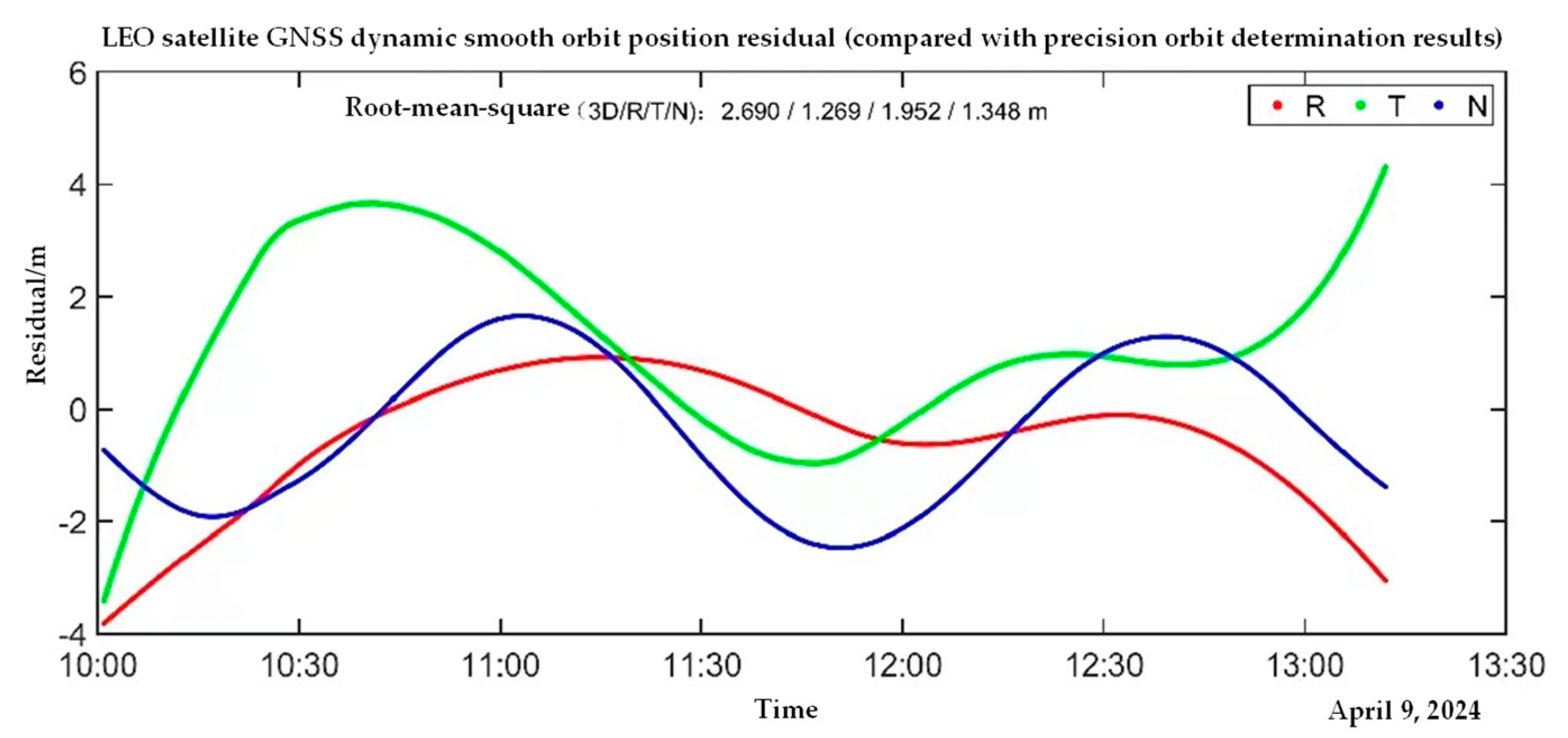
The smoothed orbit is obtained after dynamic smoothing using GNSS single-point positioning, with its accuracy shown in Figure 12. As can be seen from the figure, its accuracy is 2.69 m. The post-processing GNSS POD accuracy can reach the centimeter level.

In this experiment, the dual one-way code pseudorange from the DRO project on 9 April 2024 was used as the effective measurement data, with a time span of 3 h and 13 min and effective measurement data of 2 h and 2 min. The continuity of the observation data was only affected by Earth–Moon occultation. Specifically, the frequency of Earth–Moon occultation phenomena is related to the orbital period of the LEO satellite, resulting in approximately 0.5 h of observation interruption every 1.5 h in the inter-satellite link. During the experiment, the measurement signal strength remained stable, and the measurement data integrity rate was high.

A residual analysis method based on a priori precise orbits and high-order polynomial fitting (fifth-order Legendre orthogonal basis expansion) was used to quantitatively evaluate the measurement accuracy of inter-satellite dual one-way code pseudorange measurement data. The accuracy analysis results are shown in Figure 13.

The analysis results show that the peak-to-peak measurement noise of dual one-way pseudorange measurement does not exceed 0.2 m, with a standard deviation (STD) of 0.047 m. This indicates that the measurement accuracy of the inter-satellite link is high, providing reliable data support for autonomous orbit determination.

The Earth–Moon transfer orbit is shown in Figure 14. Satellites take a longer time to transfer in this orbit but consume less fuel. The test’s initial epoch is 9 April 2024 at 10:01 Beijing time; the duration is 3 h, 11 min, and 14 s, and the measurement interval is set to 30 s.

4.2.2. Test Result

The orbit determination parameters for the test are shown in

Table 5. Test parameters for orbit determination using actual onboard data.

Parameter	Value
initial position error of DRO-A satellite/km	$10/100 (1-\sigma$)
initial velocity error of DRO-A satellite/(m/s)	$1/10 (1-\sigma$)
initial solar pressure coefficient error	0.20
standard deviation of distance measurement error/m	0.25
process noise of DRO-A satellite (R/T/N)/(m/s2)	1 × 10−7/1 × 10−7/1 × 10−7

.

Orbit determination is performed under two initial conditions. When the initial position error of the DRO-A satellite is 10 km, its initial velocity error is 1 m/s; when the initial position error is 100 km, the initial velocity error increases by the same multiple.

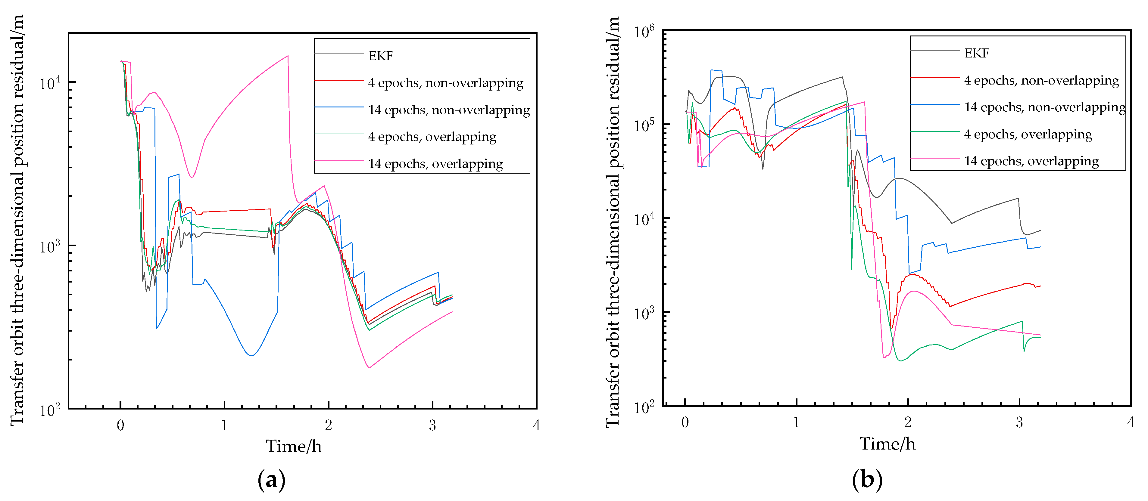
The position accuracy of the DRO-A satellite after orbit determination under different initial errors when the DRO-L satellite adopts the smoothed orbit is shown in Figure 15 and

Table 6. The orbit determination results for the DRO-A satellite’s position when its initial position error is 100 km and the positioning error of the DRO-L satellite (smoothed orbit) is 2.69 m.

Result Statistics		Algorithms
	EKF	4 Epochs, Non-Overlapping	14 Epochs, Non-Overlapping	4 Epochs, Overlapping	14 Epochs, Overlapping
Time taken to converge to within 10 km/h	3.02	1.60	2.02	1.57	1.68
Position accuracy/m	11,127.26	1863.38	5403.77	623.86	586.55

. The root mean square of the last 10 percent of the orbit determination results is calculated as an indicator of the accuracy of orbit determination. As shown in the figure and table,

(1)

When the initial position error is 10 km, there is not much difference in the performance of each algorithm, and the orbit determination residuals can converge to below 1 km within 2.23 h;

(2)

When the initial position error reaches 100 km, compared to the classic EKF, the SWBP algorithm can effectively suppress the oscillation amplitude at the beginning of orbit determination, thereby enhancing the stability of the orbit determination system. Within a limited time, this algorithm can achieve higher-precision convergence and significantly accelerate the convergence speed. In a comparison of the SWBP algorithm and the EKF algorithm, the specific performance is as follows:

①

Oscillation amplitude: The EKF oscillates to a maximum position deviation of 320.73 km during the initial orbit determination stage, while the overlapping SWBP algorithm oscillates to a maximum of only 167.73 km.

②

Convergence speed: The EKF converges to within 10 km of orbit deviation at 3.02 h, while the non-overlapping and overlapping SWBP algorithms converge to within 10 km of orbit deviation at 2.02 h and 1.68 h, respectively.

③

Convergence accuracy: Within a finite time, the EKF’s orbit determination accuracy is only 11,127.26 m, while the overlapping SWBP algorithm’s orbit determination accuracy can reach 600 m.

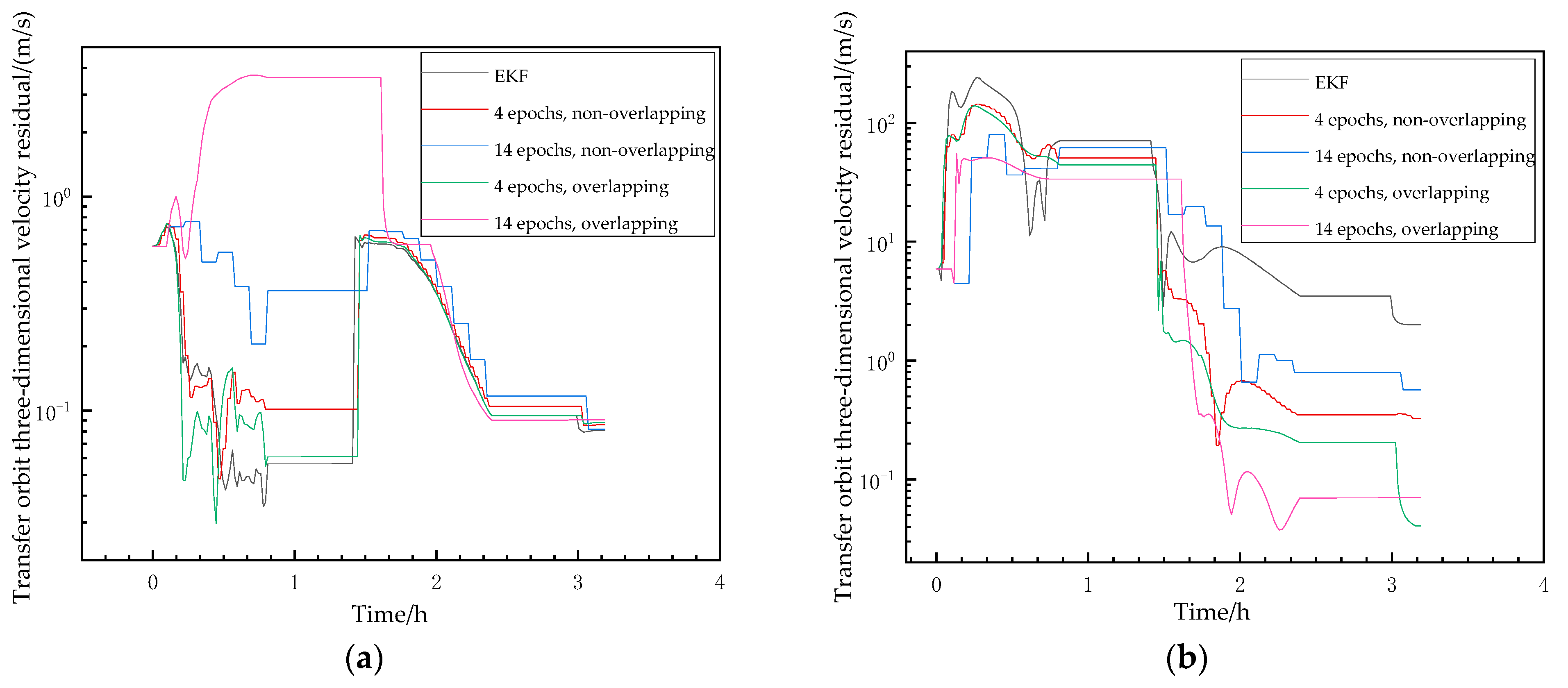
Correspondingly, the velocity results are shown in Figure 16, and the trend of the results is consistent with that of the position results. When the initial velocity error is 1 m/s, the velocity accuracy of all algorithms can reach 0.1 m/s; when the initial velocity error reaches 10 m/s, the velocity accuracy under EKF orbit determination is 2.68 m/s, while the velocity accuracy under non-overlapping and overlapping SWBP orbit determination can reach 1 m/s and 0.1 m/s, respectively.

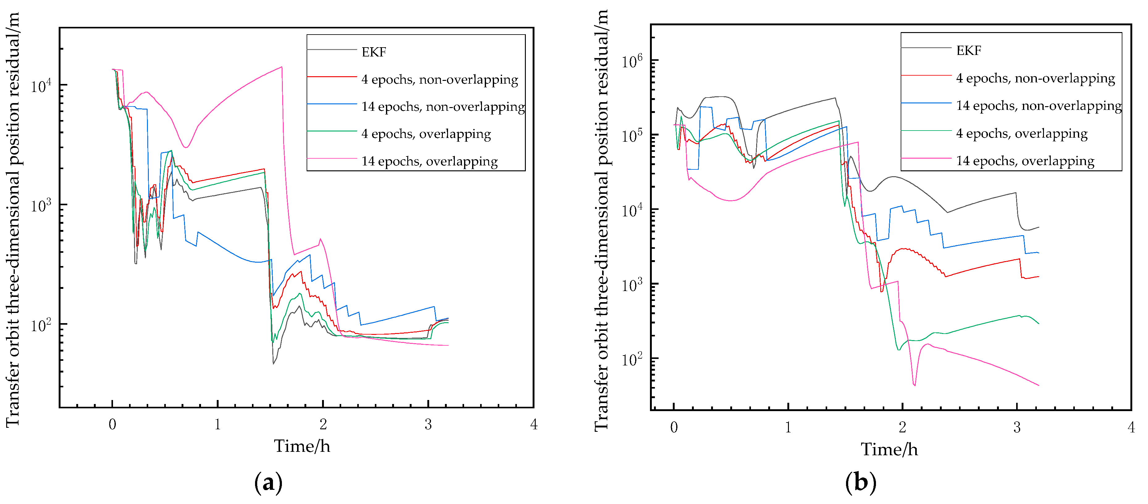
The position orbit determination results when LEO adopts a precise orbit are shown in Figure 17 and

Table 7. The orbit determination results for the DRO-A satellite’s position when its initial position error is 100 km and the positioning error of the DRO-L satellite (precision orbit) is at the centimeter level.

Result Statistics		Algorithms
	EKF	4 Epochs, Non-Overlapping	14 Epochs, Non-Overlapping	4 Epochs, Overlapping	14 Epochs, Overlapping
Time taken to converge to within 10 km/h	3.01	1.60	2.02	1.55	1.65
Position accuracy/m	10,819.05	1640.32	3591.37	338.42	71.65

, which still confirm the above conclusion. As the positioning accuracy of the DRO-L satellite improves, the orbit determination accuracy of all algorithms also improves accordingly. However, it is worth noting that the large-window non-overlapping SWBP algorithm performs poorly in the later stage. An excessively large window may result in a decrease in the frequency of measurement updates, which may weaken the effectiveness of measurement updates. Therefore, for large windows, it is recommended to adopt an overlapping sliding-window strategy with a smaller sliding step size to improve orbit determination performance.

Correspondingly, the velocity results are shown in Figure 18. Under conditions of large initial errors, the SWBP algorithm can converge to higher accuracy at a faster rate within a certain period of time. As can be seen from the figure, the velocity accuracy improves by approximately one to two orders of magnitude.

4.2.3. Discussion and Analysis

The above results show that the test results for the actual onboard data are consistent with those for the simulated data, and the main conclusions are as follows:

(1)

When the DRO-L satellite’s positioning error increases or the initial state error of the DRO-A satellite increases, the orbit determination accuracy will be degraded. When the initial position error of the DRO-A satellite is 10 km, the time required for the orbit converge to 1 km is within 2.23 h; however, when the initial position error increases to 100 km and the initial velocity error increases to 10 m/s, the SWBP significantly accelerates the convergence speed by suppressing the oscillation amplitude at the start of the orbit determination, improving the orbit determination accuracy by one to two orders of magnitude within 4 h.

(2)

The SWBP algorithm enhances the measurement update capability by utilizing more data, thereby achieving better orbit determination results. However, it is worth noting that non-overlapping SWBP with a large-window design has its measurement update capability weakened due to the reduced measurement update frequency. When this weakening effect exceeds the enhancement brought by the increased data volume, large-window non-overlapping SWBP may face the risk of degradation in orbit determination performance.

5. Conclusions

This paper proposes a Sliding-Window Batch Processing orbit determination algorithm and applies it to the scenario of space-based orbit determination. This algorithm combines the advantages of batch processing and sequential processing, and can improve the convergence speed and accuracy of orbit determination while ensuring real-time performance. The main conclusions are as follows:

(1)

When the cislunar satellite’s initial state error is small and the LEO satellite provides high-precision positioning, the SWBP algorithm shows no significant advantage over the EKF. However, when the cislunar satellite exhibits large initial state errors or the LEO satellite’s positioning accuracy degrades, the SWBP algorithm significantly improves orbit determination performance by effectively integrating additional measurement data.

(2)

Algorithm performance exhibits a clear correlation with window capacity. The larger the cislunar satellite’s initial error, the more appropriate it is to select a larger window capacity to enhance orbit correction capabilities by increasing data utilization.

(3)

The overlapping SWBP algorithm generally outperforms its non-overlapping counterpart, particularly at larger window capacities. As the window size increases, the overlapping method sustains a higher measurement update frequency, mitigating latency issues and consequently yielding superior orbit determination accuracy.

Onboard experimental results demonstrate that the SWBP algorithm maintains superior robustness against variations in orbital position errors. Consequently, this method proves capable of addressing challenging orbit determination problems while exhibiting remarkable versatility.