STHFD: Spatial–Temporal Hypergraph-Based Model for Aero-Engine Bearing Fault Diagnosis

Abstract

Accurate fault diagnosis in aerospace transmission systems is essential for ensuring equipment reliability and operational safety, especially for aero-engine bearings. However, current approaches relying on Convolutional Neural Networks (CNNs) for Euclidean data and Graph Convolutional Networks (GCNs) for non-Euclidean structures struggle to simultaneously capture heterogeneous data properties and complex spatio-temporal dependencies. To address these limitations, we propose a novel Spatial–Temporal Hypergraph Fault Diagnosis framework (STHFD). Unlike conventional graphs that model pairwise relations, STHFD employs hypergraphs to represent high-order spatial–temporal correlations more effectively. Specifically, it constructs distinct spatial and temporal hyperedges to capture multi-scale relationships among fault signals. A type-aware hypergraph learning strategy is then applied to encode these correlations into discriminative embeddings. Extensive experiments on aerospace fault datasets demonstrate that STHFD achieves superior classification performance compared to state-of-the-art diagnostic models, highlighting its potential for enhancing intelligent fault detection in complex aerospace systems.

1. Introduction

Aero-engine bearing fault diagnosis plays a critical role in maintaining the reliability and safety of aerospace transmission systems [1,2,3]. With the growing adoption of intelligent technologies in aerospace machinery, there is increasing potential to employ advanced diagnostic tools for predictive maintenance using waveform data collected from aero-engine bearing monitoring systems—such as eddy-current probes that measure low-pressure rotor displacement vibrations and accelerometers that capture acceleration vibrations on the engine casing—as provided in the widely used HIT dataset [4]. Recent advancements in deep learning have spurred the development of fault diagnosis methods that exploit multimodal data, with Convolutional Neural Networks (CNNs) and Recurrent Neural Networks (RNNs) emerging as dominant approaches [5]. These methods primarily focus on learning discriminative feature representations from various signal domains—such as time, frequency, and time–frequency—and subsequently mapping them to fault categories via multilayer neural networks. This data-driven strategy has demonstrated superior classification accuracy and automation efficiency when compared to traditional manual diagnostic techniques [6,7,8]. However, despite these advantages, CNNs and RNNs inherently rely on structured, grid-like input formats, which limits their ability to model the complex, non-Euclidean relationships that exist among sensor nodes in aerospace systems [9]. This structural limitation restricts the capacity of these models to fully exploit the spatial dependencies and topological characteristics present in real-world sensor data.

Given that sensors within aero-engine systems are functionally correlated in a non-Euclidean space, graph-based representations have been increasingly adopted to model the spatial relationships among sensor nodes [10]. Motivated by the effectiveness of Graph Convolutional Networks (GCNs) in handling graph-structured data, initial efforts employed GCNs to extract spatial–temporal features for bearing fault diagnosis [11]. In such models, each sensor channel is represented as a graph node at a given timestamp, while the connections between channels are treated as graph edges. Building on this foundation, recent research has focused on constructing spatial–temporal graph learning frameworks that jointly encode the spatial interdependencies and temporal evolution of bearing waveform data [12]. Experimental findings consistently demonstrate that these graph-based approaches surpass traditional deep learning models, such as CNNs and RNNs, in diagnostic performance [13,14]. Despite their effectiveness, a major challenge lies in designing graph structures that are both accurate and industrially meaningful. Most existing spatial–temporal graph learning models rely either on static similarity metrics—such as Phase Locking Value—to generate fixed graphs or on trainable attention weights to infer inter-node connectivity [15]. However, these approaches predominantly emphasize pairwise relationships, thus failing to capture more complex, higher-order interactions among multiple signal waveforms occurring simultaneously. This oversimplification limits their capacity to reflect the true dynamics and heterogeneity of sensor networks in aero-engine systems.

Figure 1 illustrates the fundamental structural differences between traditional graphs and hypergraphs. (a) A conventional graph is shown alongside its corresponding adjacency matrix, which captures only pairwise relationships between nodes—each edge connects exactly two vertices, and the matrix entries denote binary connections. (b) In contrast, a hypergraph is presented with its incidence matrix, where each hyperedge can simultaneously link multiple nodes. This representation enables the modeling of higher-order interactions that are not representable in standard graphs. The incidence matrix reflects node-to-hyperedge associations, allowing for a more expressive and flexible relational structure suitable for complex data scenarios. In this paper, we introduce a novel framework named Spatial–Temporal Hypergraph Fault Diagnosis (STHFD), aimed at enhancing the accuracy of fault diagnosis in aero-engine bearings. To the best of our knowledge, this work presents the first attempt to apply hypergraph-based modeling to analyze multimodal bearing signal data for fault detection in aerospace systems. The key contributions of this study are as follows:

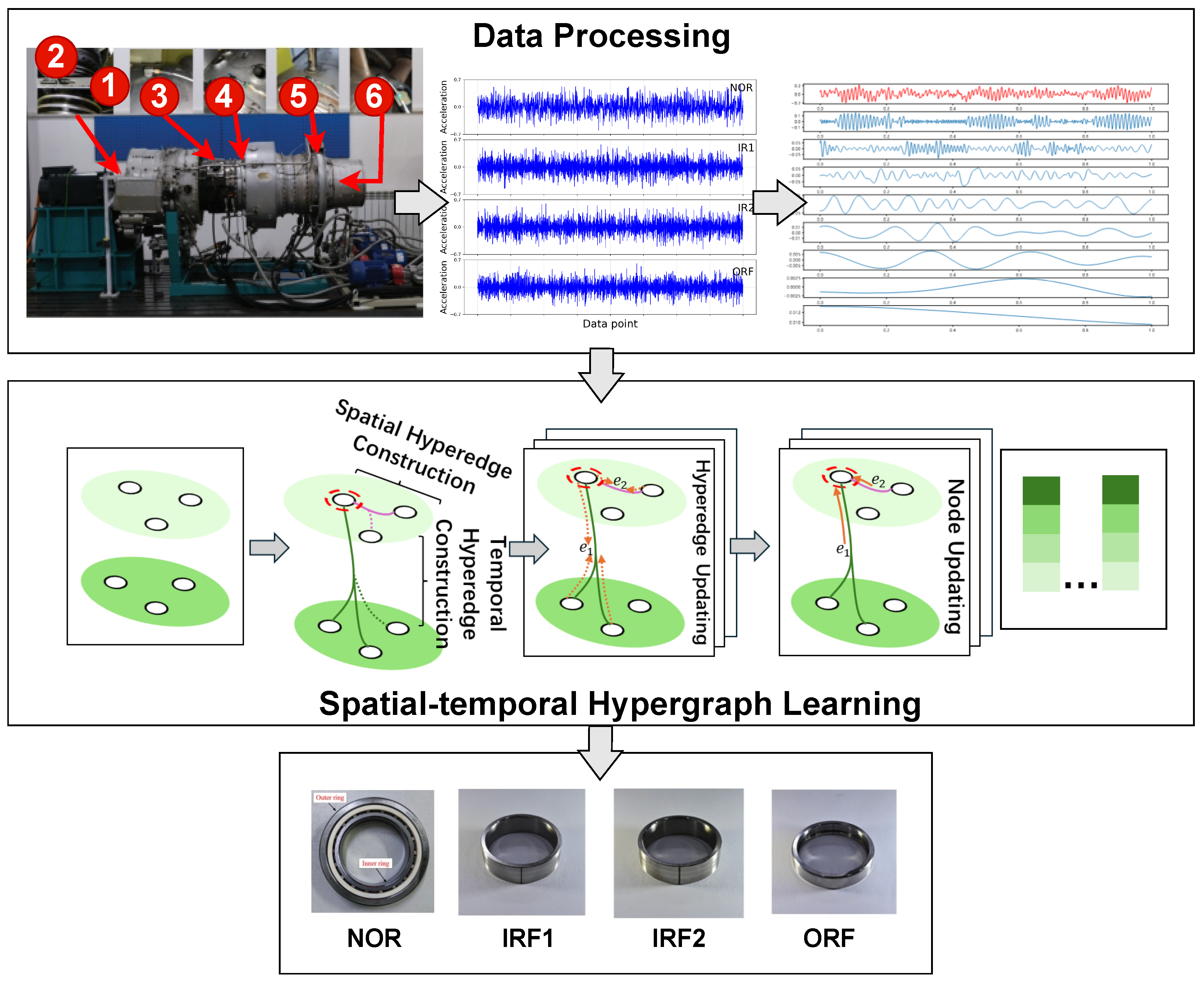
• We developed a fault diagnosis architecture that leverages hypergraphs to model high-order relationships among signal modalities. The framework supports dynamic hyperedge construction and incorporates a multi-head attention mechanism for updating node embeddings.
• A dedicated learning strategy is proposed to separately construct spatial and temporal hyperedges, allowing the framework to better represent complex dependencies in the data. The embedding update process captures both the heterogeneity and interactivity among signal nodes through attention-based aggregation.
• We evaluated the proposed STHFD framework on real-world aero-engine bearing datasets. The experimental results consistently show that our approach outperforms existing baseline models in fault classification tasks, demonstrating its robustness and practical potential.

2. Related Work

2.1. Traditional Learning Methods

The analysis of bearing signal data has attracted increasing attention in recent years, largely driven by advancements in deep learning techniques [16,17]. Prior studies have demonstrated that the effective modeling of such data holds considerable value for intelligent fault diagnosis in industrial applications [18]. However, extracting and interpreting latent patterns from these high-dimensional, temporally evolving signals remains a complex and ongoing challenge.

To overcome this, many recent approaches have focused on capturing spatial and temporal dependencies to improve classification and prediction performance [19]. For instance, several works have introduced dedicated models capable of learning intricate correlations across bearing signal channels, leading to marked improvements in diagnostic accuracy [20]. Techniques designed for multi-channel temporal data have shown promising results, particularly in regression and classification tasks. RNNs [21] have been widely employed to capture non-linear temporal dynamics, with architectures such as ConvLSTM and BiLSTM demonstrating strong capabilities in modeling sequential dependencies [22,23]. Building upon this foundation, attention-based mechanisms have been proposed to enhance the learning of long-range temporal patterns [24]. These approaches often integrate spatial and temporal attention modules to more effectively cluster and interpret multivariate time series of varying durations.

Furthermore, some studies have reported that spatial features exhibit partial time-invariance, suggesting that decoupled modeling strategies for spatial and temporal components may offer additional benefits. For example, LSBT-Net employs a two-stage pipeline, where CNNs are first used to extract spatial features, followed by LSBT-Net to model temporal transitions [25]. Similarly, hierarchical neural architectures have been proposed to separately learn spatial representations and temporal sequences, improving model interpretability and performance [26].

2.2. Graph-Based Learning Methods

While CNNs and RNNs have demonstrated notable success in processing aero-engine bearing signal data, they exhibit intrinsic limitations. These models operate within Euclidean domains, thereby neglecting the complex connectivity patterns present in spatial sensor configurations. Moreover, the learned dependencies are often difficult for domain experts to interpret due to the implicit nature of deep representations. To address these issues, Graph Neural Networks (GNNs) have emerged as a promising alternative, offering an enhanced capability to model topological structures across spatial and temporal dimensions [9].

Despite their effectiveness on non-Euclidean data, applying GNNs to aero-engine bearing signals poses several non-trivial challenges. One key difficulty lies in constructing an appropriate graph representation, which typically involves two steps: (1) defining spatial correlations among sensor signals to generate an adjacency matrix and (2) deriving informative node features from temporal signal sequences. To this end, a variety of methods have been proposed. For example, Graph Convolutional Recurrent Networks (GCRNs) combine Long Short-Term Memory (LSTM) units with Chebyshev graph filters to capture spatio-temporal patterns [27]. Structural RNN models incorporate RNNs at both node and edge levels to represent spatial interactions. Alternative approaches, such as ST-GCN, utilize partitioned graph convolution to extract spatial features and 1D convolution to model temporal dynamics [28].

However, most of these methods rely on fixed graph structures generated from static similarity measures or use trainable parameters to infer pairwise connections. These strategies, while effective to some extent, often oversimplify the true underlying structure of the signal network. In particular, they fail to capture higher-order interactions involving multiple signals simultaneously, thereby limiting the expressiveness and adaptability of the graph-based representation [29]. In contrast to the aforementioned graph-based approaches, we propose a novel framework termed Spatial–Temporal Hypergraph Fault Diagnosis (STHFD). Rather than limiting the modeling to pairwise relationships, as in conventional graph structures, STHFD leverages hypergraphs to capture high-order correlations that inherently exist in spatial–temporal fault signal data. To achieve this, the framework constructs separate spatial and temporal hyperedges, enabling it to model complex, multi-scale dependencies across sensor channels and time sequences. Furthermore, a type-aware hypergraph learning mechanism is introduced to transform these structured relationships into expressive and discriminative node embeddings, thereby enhancing the fault classification capability.

3. Methodology

This section introduces a novel framework based on a spatial–temporal hypergraph for fault diagnosis. The overall architecture of STHFD is shown in Figure 2.

3.1. Problem Definition

Let $\mathcal{D}=[{\mathbf{D}}_1,\dots ,{\mathbf{D}}_T]\in {\mathbb{R}}^{T\times C\times f}$ denote the temporal bearing signal dataset, where T is the number of time steps, C is the number of sensor channels, and f is the dimension of features per channel. At each time t, the slice ${\mathbf{D}}_t=[{\mathbf{d}}_t^{\left(1\right)},\dots ,{\mathbf{d}}_t^{\left(C\right)}]\in {\mathbb{R}}^{C\times f}$ contains the spatial features across all C channels. The label sequence is represented as $\mathbf{z}=[z_1,\dots ,z_T]$, where $z_t\in \mathcal{Z}$ is the class label of the system at time t.

We define a dynamic hypergraph ${\mathcal{H}}_t=\{{\mathcal{V}}_t,{\mathcal{E}}_t\}$ at each time step t, where each node $v_t^{\left(i\right)}\in {\mathcal{V}}_t$ corresponds to sensor channel i. Hyperedges ${\mathcal{E}}_t$ are constructed to encode spatial–temporal interactions using both current and previous timestamp data.

3.2. Dynamic Hypergraph Construction

To model cross-temporal interactions, we construct the hypergraph node set by merging the current and preceding timestamps: ${\tilde{\mathcal{V}}}_t={\mathcal{V}}_t\cup {\mathcal{V}}_{t-1}$. Each hyperedge is generated with one node designated as a master node, denoted as $v_t^{\left(i\right)}$, and a set of candidate candidate nodes from ${\tilde{\mathcal{V}}}_t$.

(1) Spatial Hyperedges: For each master node $v_t^{\left(i\right)}$, the spatial candidate set is defined as ${\mathcal{S}}_{\mathrm{spa}}\left(v_t^{\left(i\right)}\right)=\{v\in {\mathcal{V}}_t\mid v\ne v_t^{\left(i\right)}\}$. The reconstruction loss for the spatial hyperedge is

$${\mathcal{C}}_{\mathrm{spa}}^{\left(i\right)}={∥{\mathbf{d}}_t^{\left(i\right)}{\mathbf{W}}_{\mathrm{spa}}-\sum _{j=1}^{C-1}{\rho }_{\mathrm{spa}}^{\left(i\right)}\left(j\right)·{\mathbf{d}}_t^{\left(j\right)}∥}_2^2$$

(1)

Only nodes with positive coefficients ${\rho }_{\mathrm{spa}}^{\left(i\right)}\left(j\right)>0$ are included in final hyperedge ${\mathcal{E}}_{\mathrm{spa}}\left(v_t^{\left(i\right)}\right)$.

(2) Temporal Hyperedges: Similarly, for master node $v_t^{\left(i\right)}$, a temporal candidate set is selected from ${\mathcal{V}}_{t-1}$. The temporal reconstruction loss ${\mathcal{C}}_{\mathrm{tem}}^{\left(i\right)}$ is computed analogously using ${\mathit{\rho }}_{\mathrm{tem}}^{\left(i\right)}$ and ${\mathbf{W}}_{\mathrm{tem}}$.

(3) Hyperedge Generation Loss: The total reconstruction loss for time t is

$${\mathcal{L}}_{\mathrm{recon}}=\sum _{i=1}^C\lambda \left({\mathcal{C}}_{\mathrm{spa}}^{\left(i\right)}+{\mathcal{C}}_{\mathrm{tem}}^{\left(i\right)}\right)+\parallel {\mathit{\rho }}_{\mathrm{spa}}^{\left(i\right)}{\parallel }_1+{\parallel {\mathit{\rho }}_{\mathrm{tem}}^{\left(i\right)}\parallel }_1+\gamma \left(\parallel {\mathit{\rho }}_{\mathrm{spa}}^{\left(i\right)}{\parallel }_2^2+{\parallel {\mathit{\rho }}_{\mathrm{tem}}^{\left(i\right)}\parallel }_2^2\right)$$

(2)

where $\lambda$ controls the balance of reconstruction loss and $\gamma$ is a regularizer for sparsity and stability.

3.3. Hypergraph Embedding Learning

3.3.1. Hyperedge Embedding

Let $\mathbf{H}$ denote the incidence matrix with $\mathbf{H}(v,e)=1$ if v is the master node of hyperedge e, $\rho \left(v\right)$ if v is a candidate node, and 0 otherwise. The embedding of hyperedge e is obtained by

$${\mathbf{e}}_e={\displaystyle \frac{{\sum }_{v\in {\tilde{\mathcal{V}}}_t}\mathbf{H}(v,e)·\mathbf{d}\left(v\right)}{{\sum }_{v\in {\tilde{\mathcal{V}}}_t}\mathbf{H}(v,e)}}$$

(3)

3.3.2. Multi-Head Attention for Node Updating

Each node $v_t^{\left(i\right)}$ aggregates information from its corresponding spatial and temporal hyperedges via multi-head attention. For the k-th head,

$$\begin{array}{cc}\hfill {\mathbf{q}}^{\left(k\right)}& ={\mathbf{d}}_t^{\left(i\right)}{\mathbf{W}}_q^{\left(k\right)},{\mathbf{k}}^{\left(k\right)}={\mathbf{e}}_{\mathrm{spa}}^{\left(i\right)}{\mathbf{W}}_k^{\left(k\right)}\hfill \end{array}$$

(4)

$$\begin{array}{cc}\hfill {\alpha }_{\mathrm{spa}}^{\left(k\right)}& ={\displaystyle \frac{{\mathbf{q}}^{\left(k\right)}{\mathbf{W}}_a^{\left(k\right)}{\left({\mathbf{k}}^{\left(k\right)}\right)}^{\top }}{\sqrt{f/K}}},{\omega }_{\mathrm{spa}}^{\left(k\right)}=\mathrm{softmax}\left({\alpha }_{\mathrm{spa}}^{\left(k\right)}\right)\hfill \end{array}$$

(5)

Likewise, temporal weights ${\omega }_{\mathrm{tem}}^{\left(k\right)}$ are computed. Final node embedding is updated as

$${\mathbf{z}}_t^{\left(i\right)}=\mathrm{FC}\left({\parallel }_{k=1}^K\left({\omega }_{\mathrm{spa}}^{\left(k\right)}{\mathbf{k}}_{\mathrm{spa}}^{\left(k\right)}+{\omega }_{\mathrm{tem}}^{\left(k\right)}{\mathbf{k}}_{\mathrm{tem}}^{\left(k\right)}\right)\right)$$

(6)

3.3.3. Graph Readout and Final Prediction

The hypergraph representation is computed by averaging node embeddings:

$${\mathbf{z}}_{{\mathcal{H}}_t}={\displaystyle \frac{1}{C}}\sum _{i=1}^C{\mathbf{z}}_t^{\left(i\right)}$$

(7)

The final output is obtained via a fully connected classifier. The end-to-end training loss is

$$\mathcal{L}=\alpha {\mathcal{L}}_{\mathrm{recon}}+(1-\alpha )·{\mathcal{L}}_{\mathrm{cls}}({\mathbf{z}}_{{\mathcal{H}}_t},z_t)$$

(8)

where ${\mathcal{L}}_{\mathrm{cls}}$ is the cross-entropy classification loss and $\alpha$ controls the trade-off between structure learning and classification objectives.

4. Experiments

To comprehensively evaluate the effectiveness and robustness of the proposed STHFD framework, we formulate the following research questions. These questions are designed to guide the experimental evaluation by addressing three key aspects: (1) overall diagnostic performance compared to existing methods, (2) the model’s capability to distinguish between different fault types, and (3) the individual contributions of core components within the architecture. We answer these questions through extensive experiments, including performance benchmarking, confusion matrix analysis, and ablation studies.

• RQ1: How does the proposed STHFD model compare with existing baseline methods in terms of diagnostic accuracy and robustness?
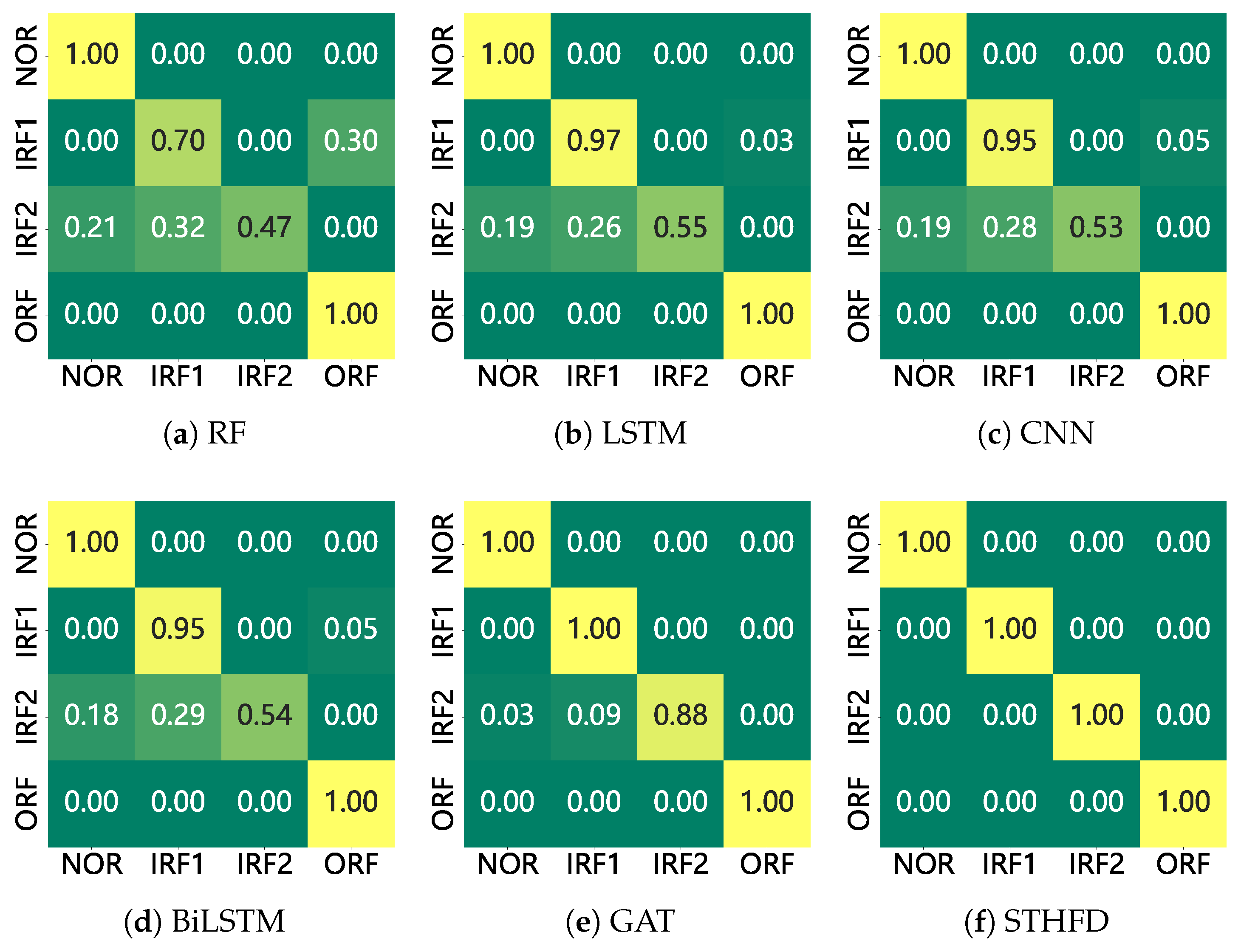
• RQ2: To what extent can different models distinguish between fault categories, and what are the common patterns of class-wise misclassification?
• RQ3: How does each component of the proposed model contribute to its overall performance?

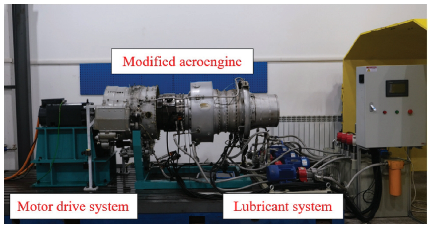
4.1. Dataset

The experimental data used in this study were derived from the HIT inter-shaft bearing fault dataset [4], which was collected using a real aero-engine core assembly. The test rig included a motor-driven unit operating at a fixed rotational speed of 6000 rpm, with bearings under operational load and a fully integrated lubrication system to closely mimic in-service conditions. The system was instrumented with six sensors: two eddy current probes mounted near the low-pressure rotor to capture displacement vibrations and four accelerometers mounted on the engine casing to collect acceleration vibration data. The sensor layout is depicted in Figure 2. The bearing types under investigation were inter-shaft bearings, and four fault conditions were studied: normal (NOR), inner ring fault 1 (IRF1), inner ring fault 2 (IRF2), and outer ring fault (ORF). Artificial damage was introduced to simulate realistic fault modes. Specifically, IRF1 and ORF featured 0.5 mm length × 0.5 mm depth defects, while IRF2 had a 1 mm length × 0.5 mm depth defect. These sizes represented approximately 1–2% of the raceway width, aligning with early fault detection scenarios in practice.

Each raw sample corresponded to a 15 s vibration sequence recorded at a sampling rate of 25,000 Hz. After segmentation and preprocessing, the dataset comprised 2412 labeled signal groups, each containing 20,480 data points. An overview of the experimental setup is illustrated in Figure 2, where the locations of the six sensors are clearly marked on the leftmost subfigure. The test rig, based on a real aero-engine, is shown in Figure 3.

Compared to simulated datasets, the HIT dataset reflected more realistic and complex signal characteristics, which pose greater challenges for intelligent diagnostic models. For model training and evaluation, we split the dataset into a training set and a test set at a ratio of 7:3. Figure 4 shows time domain examples of NOR, IRF1, IRF2, and ORF, respectively. Furthermore, Figure 5 presents samples processed via Empirical Mode Decomposition (EMD), illustrating signal mode components used for spatial–temporal node constructs.

4.2. Model Configuration

All experiments were conducted on a high-performance workstation equipped with an Intel Core i9-13900K CPU with 128 GB of DDR5 RAM and an NVIDIA GeForce RTX 4090 GPU with 24 GB of VRAM. The software environment included Python 3.6 and PyTorch 2.1.2, running with CUDA Toolkit version 12.1. To ensure result reproducibility, all experiments were executed with fixed random seeds.

4.3. Comparison Methods

To validate the effectiveness of our proposed STHFD framework, we compared it against five representative baseline methods, covering both classical machine learning algorithms and modern deep learning architectures:

• (1) RF [30]: Random Forest, a widely used ensemble learning algorithm that constructs multiple decision trees and aggregates their predictions via majority voting.
• (2) CNN [31]: A 1D Convolutional Neural Network designed to capture local temporal patterns in vibration signals.
• (3) LSTM [31]: A Long Short-Term Memory network capable of modeling long-range temporal dependencies within sequential data.
• (4) BiLSTM [23]: A bidirectional variant of LSTM that processes a sequence in both forward and backward directions to enhance contextual feature learning.
• (5) GCN [32]: A Graph Convolutional Network that utilizes spatial graph structures constructed from sensor topology to model inter-channel dependencies.

For all baseline models, we followed the preprocessing steps, network structures, and optimization strategies as described in their respective original publications. Hyperparameter tuning was performed independently for each method using a validation subset split from the training data. Specifically, the learning rate was selected from the candidate set $\{0.1,0.05,0.01,0.005,0.001,0.0001\}$ based on validation accuracy. For the proposed STHFD model, the key hyperparameters in the reconstruction loss function were set as follows: the reconstruction error weight $\lambda$ was fixed at 0.01, the regularization coefficient $\gamma$ was set to 0.2, and the overall loss balance parameter $\alpha$ was assigned a value of 0.1.

4.4. Experiment Results and Analysis

4.4.1. Performance Comparison (RQ1)

To gain deeper insight into the diagnostic capabilities of each model, we report the per-class precision, recall, and F1-score in

Table 1. Per-class precision, recall, and F1-score for each method.

Class	Metric	RF	LSTM	CNN	BiLSTM	GCN	STHFD
1	Precision	0.8154	0.8167	0.8226	0.8413	0.9623	1.0000
	Recall	1.0000	1.0000	1.0000	1.0000	1.0000	1.0000
	F1-score	0.8983	0.8991	0.9027	0.9138	0.9808	1.0000
2	Precision	0.7000	0.8000	0.7838	0.9138	0.9242	1.0000
	Recall	0.7000	0.9677	0.9508	0.9516	1.0000	1.0000
	F1-score	0.7000	0.8759	0.8593	0.8613	0.9606	1.0000
3	Precision	1.0000	1.0000	1.0000	1.0000	1.0000	1.0000
	Recall	0.4737	0.5517	0.5345	0.5357	0.8793	1.0000
	F1-score	0.6429	0.7111	0.6966	0.5357	0.9358	1.0000
4	Precision	0.7500	0.9649	0.9474	0.9464	1.0000	1.0000
	Recall	1.0000	1.0000	1.0000	1.0000	1.0000	1.0000
	F1-score	0.8571	0.9821	0.9730	0.9725	1.0000	1.0000

. Across all four fault categories, the proposed STHFD framework consistently achieved perfect scores (1.0000) in all metrics, demonstrating its superior ability to capture discriminative features and correctly classify fault types without error. The GCN also performed competitively, especially in Class 1 and Class 4, where it achieved perfect recall and precision. However, its performance in Class 3 was noticeably lower in terms of recall (0.8793) and F1-score (0.9358), indicating challenges in detecting subtle patterns in that category. This suggests that while GCN can model spatial dependencies, it may be limited in capturing higher-order temporal interactions. Traditional deep learning models such as LSTM, CNN, and BiLSTM performed moderately well. For instance, BiLSTM achieved an F1-score of 0.9725 in Class 4 but underperformed in Class 3, with an F1-score of only 0.5357. Similarly, LSTM and CNN exhibited lower recall values in Class 3, reflecting difficulty in identifying this fault type reliably. RF, representing a classical machine learning baseline, showed the weakest performance overall, particularly in Class 2 and Class 3, where its F1-scores dropped to 0.7000 and 0.6429, respectively. STHFD achieved 100% precision, recall, and F1-score across all four fault categories, whereas the best-performing baseline (GCN) fell short in Class 3 (IRF2), with a recall of 0.8793 and an F1-score of 0.9358. This demonstrated that STHFD achieved an average F1-score improvement of 6.5% over GCN and more than 20% improvement over LSTM and CNN. These gains indicate the model’s enhanced ability to capture subtle spatial–temporal patterns and fault-specific features, which are often missed by pairwise or sequential models.

Overall, the results validate the effectiveness of our proposed STHFD model in delivering stable and accurate classification across all fault categories, outperforming both classical and deep learning baselines. Its ability to model complex spatial–temporal dependencies through hypergraph representations is the key contributing factor to this performance. Moreover, while the STHFD framework achieved perfect classification metrics (Table 1), this result was not due to overfitting. The dataset used is publicly available and the training/testing split ensured no data leakage. Moreover, ablation studies confirmed that the model’s full architecture was necessary to achieve this level of performance, and performance degraded when key components were removed. The consistent improvements across all fault classes, particularly those with subtle differences (e.g., IRF1 vs. IRF2), reflect the model’s capacity to generalize rather than memorize. These findings collectively support the robustness of the proposed approach.

4.4.2. Confusion Pattern Analysis (RQ2)

To further investigate the classification behavior of each method, we analyzed the confusion matrices shown in Figure 6. These visualizations provide a detailed view of how each model performed at the class level and where misclassifications commonly occurred. For traditional models such as RF and LSTM (Figure 6a,b), significant confusion was observed between the inner ring fault classes (IRF1 and IRF2). For example, RF showed substantial misclassification from IRF2 to IRF1 (32%) and NOR (21%), indicating poor sensitivity to subtle signal differences. LSTM improved the recall of IRF1 to 97%, yet still confused IRF2 with other classes, particularly IRF1 and NOR. CNN and BiLSTM (Figure 6c,d) offered moderate improvements, with BiLSTM reducing cross-class confusion between IRF1 and IRF2, though misclassification from IRF2 to IRF1 remained at 29%. Additionally, both models maintained high accuracy for the NOR and ORF categories, suggesting that these fault types are more distinguishable. The GAT model (Figure 6e) showed stronger intra-class discrimination, achieving 88% accuracy for IRF2 while maintaining perfect precision for other classes. This indicates that leveraging graph attention enhances the model’s ability to learn more informative representations of fault features. Our proposed STHFD model (Figure 6f) achieved perfect classification across all categories, with no misclassified instances. This result confirms the model’s robustness in capturing both spatial heterogeneity and temporal continuity via hypergraph learning. Unlike other models, STHFD effectively separated closely related fault classes such as IRF1 and IRF2, demonstrating a clear advantage in minimizing inter-class confusion.

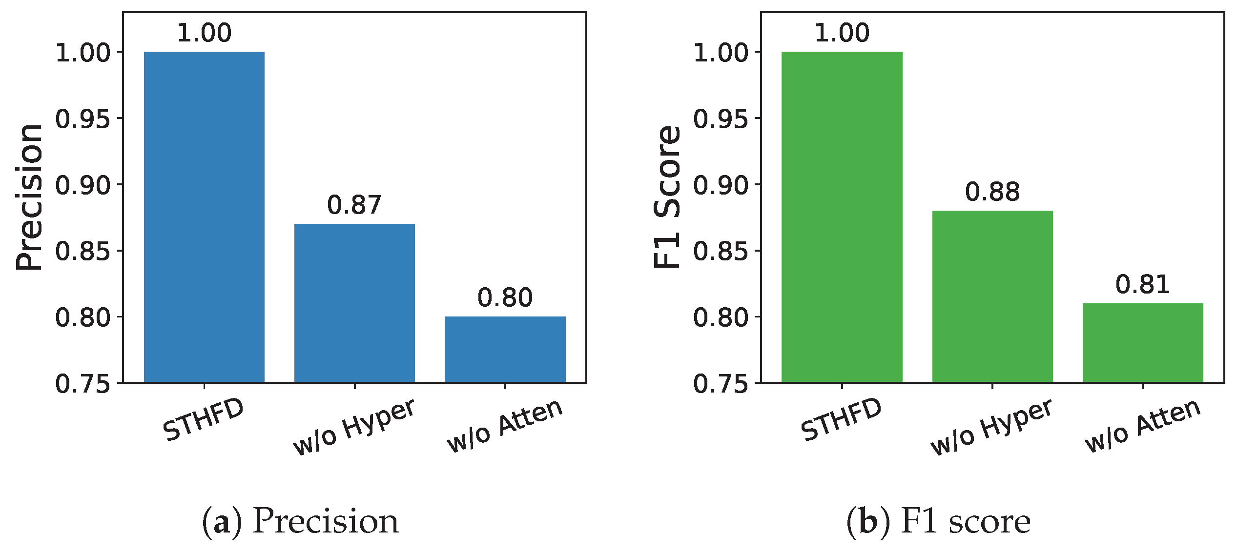
4.4.3. Ablation Study (RQ3)

To investigate the contribution of key components within the proposed STHFD framework, we performed an ablation study by selectively removing the spatial–temporal hyperedges and the attention mechanism. The results are illustrated in Figure 7, where both precision and F1 score are reported under each model setting. The complete STHFD model achieved perfect scores of 1.00 in both precision and F1 score, demonstrating its robust performance in classifying all fault types with no misclassification. When the hyperedge module was removed (w/o Hyper), the precision and F1 score dropped significantly to 0.87 and 0.88, respectively. This result highlights the importance of explicitly modeling high-order spatial–temporal relationships among nodes, which cannot be fully captured by pairwise interactions alone. On the other hand, removing the attention mechanism (w/o Atten) led to a further degradation in performance, with the F1 score dropping to 0.81 and precision to 0.80. This suggests that the attention mechanism plays a complementary role by enabling the model to selectively focus on more informative hyperedges during embedding aggregation. Overall, removing the hypergraph structure resulted in a 13% drop in F1-score, while excluding attention led to a 19% drop. These findings confirm that both dynamic hyperedge construction and attention-based aggregation are crucial to the effectiveness of STHFD. The synergy between these components ensures the model’s ability to capture fault patterns while maintaining high classification precision and robustness.

5. Conclusions

In this paper, we proposed a novel fault diagnosis framework named STHFD, which leverages spatial–temporal hypergraph learning for the accurate and robust classification of aero-engine bearing faults. Unlike traditional graph-based models that focus on pairwise relationships, STHFD constructs dynamic spatial and temporal hyperedges to capture higher-order dependencies among multi-channel vibration signals. By incorporating a multi-head attention mechanism, the model further enhances node embedding by focusing on informative interactions across time and space. Extensive experiments on a real-world aero-engine bearing dataset demonstrated that STHFD significantly outperforms existing classical and deep learning baselines in terms of precision, recall, and F1-score. A confusion matrix analysis revealed that STHFD can effectively distinguish closely related fault types, such as IRF1 and IRF2, which are often misclassified by other models. Furthermore, ablation studies confirmed that both the hyperedge construction and attention-based aggregation were essential to the model’s effectiveness, with noticeable performance drops observed when either component was removed.

References

1. Zhao, D.; Cai, W.; Cui, L. Adaptive thresholding and coordinate attention-based tree-inspired network for aero-engine bearing health monitoring under strong noise. Adv. Eng. Inform. 2024, 61, 102559. [Google Scholar] [CrossRef]
2. Wang, Z.; Luo, Q.; Chen, H.; Zhao, J.; Yao, L.; Zhang, J.; Chu, F. A high-accuracy intelligent fault diagnosis method for aero-engine bearings with limited samples. Comput. Ind. 2024, 159, 104099. [Google Scholar] [CrossRef]
3. Chai, B.X.; Gunaratne, M.; Ravandi, M.; Wang, J.; Dharmawickrema, T.; Di Pietro, A.; Jin, J.; Georgakopoulos, D. Smart industrial internet of things framework for composites manufacturing. Sensors 2024, 24, 4852. [Google Scholar] [CrossRef] [PubMed]
4. Hou, L.; Yi, H.; Jin, Y.; Gui, M.; Sui, L.; Zhang, J.; Chen, Y. Inter-shaft bearing fault diagnosis based on aero-engine system: A benchmarking dataset study. J. Dyn. Monit. Diagn. 2023, 2, 228–242. [Google Scholar] [CrossRef]
5. Huang, T.; Zhang, Q.; Tang, X.; Zhao, S.; Lu, X. A novel fault diagnosis method based on CNN and LSTM and its application in fault diagnosis for complex systems. Artif. Intell. Rev. 2022, 55, 1289–1315. [Google Scholar] [CrossRef]
6. Ruan, D.; Wang, J.; Yan, J.; Gühmann, C. CNN parameter design based on fault signal analysis and its application in bearing fault diagnosis. Adv. Eng. Inform. 2023, 55, 101877. [Google Scholar] [CrossRef]
7. Wang, Y.; Xu, S.; Bwar, K.; Eisenbart, B.; Lu, G.; Belaadi, A.; Fox, B.; Chai, B. Application of machine learning for composite moulding process modelling. Compos. Commun. 2024, 48, 101960. [Google Scholar] [CrossRef]
8. Chai, B.; Eisenbart, B.; Nikzad, M.; Fox, B.; Blythe, A.; Bwar, K.H.; Wang, J.; Du, Y.; Shevtsov, S. Application of KNN and ANN Metamodeling for RTM filling process prediction. Materials 2023, 16, 6115. [Google Scholar] [CrossRef]
9. Yu, Z.; Zhang, C.; Deng, C. An improved GNN using dynamic graph embedding mechanism: A novel end-to-end framework for rolling bearing fault diagnosis under variable working conditions. Mech. Syst. Signal Process. 2023, 200, 110534. [Google Scholar] [CrossRef]
10. Hou, D.; Zhang, B.; Chen, J.; Shi, P. Improved GNN based on Graph-Transformer: A new framework for rolling mill bearing fault diagnosis. Trans. Inst. Meas. Control 2024, 46, 2804–2815. [Google Scholar] [CrossRef]
11. Zhang, S.; Tong, H.; Xu, J.; Maciejewski, R. Graph convolutional networks: A comprehensive review. Comput. Soc. Netw. 2019, 6, 11. [Google Scholar] [CrossRef] [PubMed]
12. Guo, L.; Shi, H.; Tan, S.; Song, B.; Tao, Y. A knowledge-driven spatial-temporal graph neural network for quality-related fault detection. Process. Saf. Environ. Prot. 2024, 184, 1512–1524. [Google Scholar] [CrossRef]
13. Yang, C.; Zhou, K.; Liu, J. SuperGraph: Spatial-temporal graph-based feature extraction for rotating machinery diagnosis. IEEE Trans. Ind. Electron. 2021, 69, 4167–4176. [Google Scholar] [CrossRef]
14. Wang, L.; Xie, F.; Zhang, X.; Jiang, L.; Huang, B. Spatial-temporal graph feature learning driven by time–frequency similarity assessment for robust fault diagnosis of rotating machinery. Adv. Eng. Inform. 2024, 62, 102711. [Google Scholar] [CrossRef]
15. Wang, Z.; Tong, Y.; Heng, X. Phase-locking value based graph convolutional neural networks for emotion recognition. IEEE Access 2019, 7, 93711–93722. [Google Scholar] [CrossRef]
16. Wang, J.; Jin, J.; Zhang, T.; Chai, B.X.; Di Pietro, A.; Georgakopoulos, D. Leveraging Auxiliary Task Relevance for Enhanced Bearing Fault Diagnosis through Curriculum Meta-learning. IEEE Sens. J. 2025, 25, 22467–22478. [Google Scholar] [CrossRef]
17. Marzat, J.; Piet-Lahanier, H.; Damongeot, F.; Walter, E. Model-based fault diagnosis for aerospace systems: A survey. Proc. Inst. Mech. Eng. Part G J. Aerosp. Eng. 2012, 226, 1329–1360. [Google Scholar] [CrossRef]
18. Fekih, A. Fault diagnosis and fault tolerant control design for aerospace systems: A bibliographical review. In Proceedings of the 2014 American Control Conference, Portland, OR, USA, 4–6 June 2014; IEEE: Piscataway, NJ, USA, 2014; pp. 1286–1291. [Google Scholar]
19. Wang, T.; Liu, Z.; Lu, G.; Liu, J. Temporal-spatio graph based spectrum analysis for bearing fault detection and diagnosis. IEEE Trans. Ind. Electron. 2020, 68, 2598–2607. [Google Scholar] [CrossRef]
20. Li, D.; Wang, Y.; Wang, J.; Wang, C.; Duan, Y. Recent advances in sensor fault diagnosis: A review. Sens. Actuators A Phys. 2020, 309, 111990. [Google Scholar] [CrossRef]
21. Zhu, J.; Jiang, Q.; Shen, Y.; Qian, C.; Xu, F.; Zhu, Q. Application of recurrent neural network to mechanical fault diagnosis: A review. J. Mech. Sci. Technol. 2022, 36, 527–542. [Google Scholar] [CrossRef]
22. Wang, J.; Yang, S.; Liu, Y.; Wen, G. Deep subdomain transfer learning with spatial attention ConvLSTM network for fault diagnosis of wheelset bearing in high-speed trains. Machines 2023, 11, 304. [Google Scholar] [CrossRef]
23. Nacer, S.M.; Nadia, B.; Abdelghani, R.; Mohamed, B. A novel method for bearing fault diagnosis based on BiLSTM neural networks. Int. J. Adv. Manuf. Technol. 2023, 125, 1477–1492. [Google Scholar] [CrossRef]
24. Lv, H.; Chen, J.; Pan, T.; Zhang, T.; Feng, Y.; Liu, S. Attention mechanism in intelligent fault diagnosis of machinery: A review of technique and application. Measurement 2022, 199, 111594. [Google Scholar] [CrossRef]
25. Duan, Y.; Yang, T.; Wang, C.; Zhang, Y.; Han, Q.; Guo, S. LSBT-Net: A lightweight framework for fault diagnosis of bearings based on an interpretable spatial-temporal model. Expert Syst. Appl. 2025, 281, 127718. [Google Scholar] [CrossRef]
26. Kim, K.H.; Park, J.K. Application of hierarchical neural networks to fault diagnosis of power systems. Int. J. Electr. Power Energy Syst. 1993, 15, 65–70. [Google Scholar] [CrossRef]
27. Lv, F.; Bi, X.; Xu, Z.; Zhao, J. Causality-embedded reconstruction network for high-resolution fault identification in chemical process. Process. Saf. Environ. Prot. 2024, 186, 1011–1033. [Google Scholar] [CrossRef]
28. Li, C.; Mo, L.; Yan, R. Rotating machinery fault diagnosis based on spatial-temporal GCN. In Proceedings of the 2021 International Conference on Sensing, Measurement & Data Analytics in the era of Artificial Intelligence (ICSMD), Nanjing, China, 21–23 October 2021; IEEE: Piscataway, NJ, USA, 2021; pp. 1–6. [Google Scholar]
29. Wang, J.; Zhang, T.; Zhang, L.; Bai, Y.; Li, X.; Jin, J. HyperMAN: Hypergraph-enhanced Meta-learning Adaptive Network for Next POI Recommendation. arXiv 2025, arXiv:2503.22049. [Google Scholar]
30. Yang, B.S.; Di, X.; Han, T. Random forests classifier for machine fault diagnosis. J. Mech. Sci. Technol. 2008, 22, 1716–1725. [Google Scholar] [CrossRef]
31. Pan, H.; He, X.; Tang, S.; Meng, F. An improved bearing fault diagnosis method using one-dimensional CNN and LSTM. J. Mech. Eng./Stroj. Vestn. 2018, 64, 443–453. [Google Scholar]
32. Li, C.; Mo, L.; Yan, R. Fault diagnosis of rolling bearing based on WHVG and GCN. IEEE Trans. Instrum. Meas. 2021, 70, 1–11. [Google Scholar] [CrossRef]
Figure 1. Illustration of the structural difference between traditional graphs and hypergraphs. (a) A graph with respective adjacency matrix, which models only pairwise relationships among nodes. (b) A hypergraph and its incidence matrix, where each hyperedge can connect multiple nodes simultaneously, enabling the modeling of high-order relationships.
Aerospace 12 00612 g001
Figure 2. An overview of STHFD.
Aerospace 12 00612 g002
Figure 3. The test rig based on a real aero-engine.
Aerospace 12 00612 g003
Figure 4. Signal waveforms of each bearing.
Aerospace 12 00612 g004
Figure 5. Signal waveforms after EMD.
Aerospace 12 00612 g005
Figure 6. Confusion matrix of all compared methods.
Aerospace 12 00612 g006
Figure 7. Ablation study.
Aerospace 12 00612 g007