A Stackelberg Game Approach to Model Reference Adaptive Control for Spacecraft Pursuit–Evasion

Abstract

A Stackelberg equilibrium–based Model Reference Adaptive Control (MSE) method is proposed for spacecraft Pursuit–Evasion (PE) games with incomplete information and sequential decision making under a non–zero–sum framework. First, the spacecraft PE dynamics under $J_2$ perturbation are mapped to a dynamic Stackelberg game model. Next, the Riccati equation solves the equilibrium problem, deriving the evader’s optimal control strategy. Finally, a model reference adaptive algorithm enables the pursuer to dynamically adjust its control gains. Simulations show that the MSE strategy outperforms Nash Equilibrium (NE) and Single–step Prediction Stackelberg Equilibrium (SSE) methods, achieving 25.46% faster convergence than SSE and 39.11% lower computational cost than NE.

1. Introduction

The rapid development of space technology has increased the importance of spacecraft in many fields such as space exploration, satellite communication, and military reconnaissance [1,2,3]. At the same time, the problem of Pursuit–Evasion (PE) games between spacecraft has become increasingly significant [4]. In mission scenarios such as satellite formation flight, space debris cleanup, and space confrontation, the development of strategies to achieve efficient pursuit has become a key technical challenge [5,6,7]. For example, in satellite formation flight, each satellite must maintain a specific relative position relationship. Once there is a deviation, it is necessary to return the satellite to a predetermined orbit with the help of reasonable control strategies. This involves a decision–making process similar to that of evasion tracking [8]. In space debris cleanup missions, the pursuer has to develop a strategy to approach and capture debris, which can be regarded as a target with the intention of evasion [9]. It is these practical application requirements that drive the in–depth investigation of the spacecraft PE game problem.

When modeling the PE game problem, traditional control methods usually construct it as a special structure, a competitive scenario where the total of the pursuer’s and evader’s cost functions equals zero, essentially representing a zero–sum dynamic [10]. In recent years, the study of zero–sum games has attracted extensive attention from many scholars. Within this framework, the ultimate equilibrium state of the PE game converges at a saddle point, with the determination of this saddle point balance achieved through the solution of the Hamilton–Jacobi–Isaacs (HJI) equation [11]. In the literature [12], the scholar crafted an integral reinforcement learning algorithm tailored for a category of zero–sum differential game issues, characterized by entirely unknown dynamic attributes of the linear system. Reference [13] broadens the investigative horizon by applying the zero–sum game concept to nonlinear systems. It innovatively integrates neural network methodologies into adaptive dynamic programming, thereby effectively deriving the saddle–point equilibrium solution within such nonlinear frameworks. The study in [14] also focuses on the nonlinear zero–sum differential game problem and proposes a model–free control algorithm based on neural networks, which provides new ideas and methods for solving such problems. However, in practical situations, the goals of pursuers and evaders are not completely opposite, which leads to overly aggressive strategy design, neglects the reasonable allocation of safety and resources, and limits the flexibility of strategy design. In some cases, the zero–sum framework can lead to moral and ethical dilemmas as it encourages absolute victory for one party without considering the loss of the other [15].

While zero–sum games simplify analysis, they often fail to capture real–world scenarios where objectives are not strictly adversarial. In contrast, non–zero–sum frameworks accommodate partial competition and cooperation, enabling strategies that balance safety, fuel efficiency, and mission success; a non–zero–sum framework more accurately models the complex interplay of competition and potential cooperation between the two parties. It allows for more flexible strategies that can adapt to different mission requirements and consider long–term stability [16,17]. This has led to the development of methods like Q–learning for non–zero–sum games with incomplete information [18] and optimal continuous thrust strategies within a differential game framework [19].

A significant challenge in PE games is the inherent asymmetry of information and the sequential nature of decision making. Most traditional game–theoretic solutions are based on the Nash Equilibrium (NE), which assumes that players act simultaneously with full knowledge of each other’s strategies [20]. This assumption is often invalid in practice, as information gathering and decision making involve inherent time lags. A more suitable theoretical basis is the Stackelberg equilibrium, which models sequential decision making [21]. In the PE context, the evader often acts as the “leader”, making a move first, while the pursuer is the “follower”, reacting to the leader’s action. Therefore, the PE game is more accurately modeled as a dynamic Stackelberg game [22]. While prior works have applied Stackelberg models to surface vehicles [23] and spacecraft using single–step prediction [24], our work distinguishes itself by integrating a Model Reference Adaptive Control architecture. This approach allows the pursuer to dynamically adjust its control gains based on a reference model of the evader’s optimal strategy, offering enhanced robustness against unmodeled dynamics and disturbances, which is a primary focus of this paper.

Recent approaches to spacecraft pursuit–evasion under $J_2$ perturbations [24] typically employ linearized approximations and fixed–gain control, resulting in suboptimal tracking performance. Our Stackelberg game–based framework introduces three key innovations, as detailed in

Table 1. Comparative analysis with state–of–the–art approaches.

Category	Liu [24]	Proposed Method	Advancement
J2 Handling	Linearized approximation Offline pre–compensation	Nonlinear coupling preservation Real–time adaptive rejection	62% lower position error Exact ${sin}^2\left(kt\right)$ terms
Control Strategy	Fixed–gain controller Single–step prediction	Dynamic gain adjustment Multi–horizon optimization	22% fuel saving $fal(·)$ adaptation
Stability	Local convergence	Global UUB (Theorem 1)	Guaranteed $O\left(N{n}^3\right)$ PE-conditioned
Computation	26.5 ms/step	24.8 ms/step	6.42% faster than SSE Parallelizable

. (1) Nonlinear $J_2$ coupling preservation reduces position errors by 62% through exact ${sin}^2\left(kt\right)$ modeling. (2) Dynamic $fal(·)$ adaptation enables 22% fuel savings via multi–horizon optimization. (3) Global stability is guaranteed (Theorem 1), overcoming local convergence limitations. While the proposed method operates at 24.8 ms/step compared to 18.7 ms/step in [24], it achieves 6.42% faster execution than the SSE baseline (26.5 ms/step) through parallel computation.

The main contributions of this paper are as follows:

1.

In a non–zero–sum framework, a Stackelberg equilibrium–based Model Reference Adaptive Control (MSE) method is proposed for the spacecraft PE game. This method incorporates the dynamic Stackelberg equilibrium game model and uses the Riccati equation to derive the optimal control strategy for the evader. Subsequently, an adaptive control algorithm enables the pursuer to adjust its control gains adaptively. This approach is novel, as it specifically addresses the challenges of $J_2$ perturbations and non–zero–sum game dynamics within the PE context, which has not been thoroughly explored in prior literature.

2.

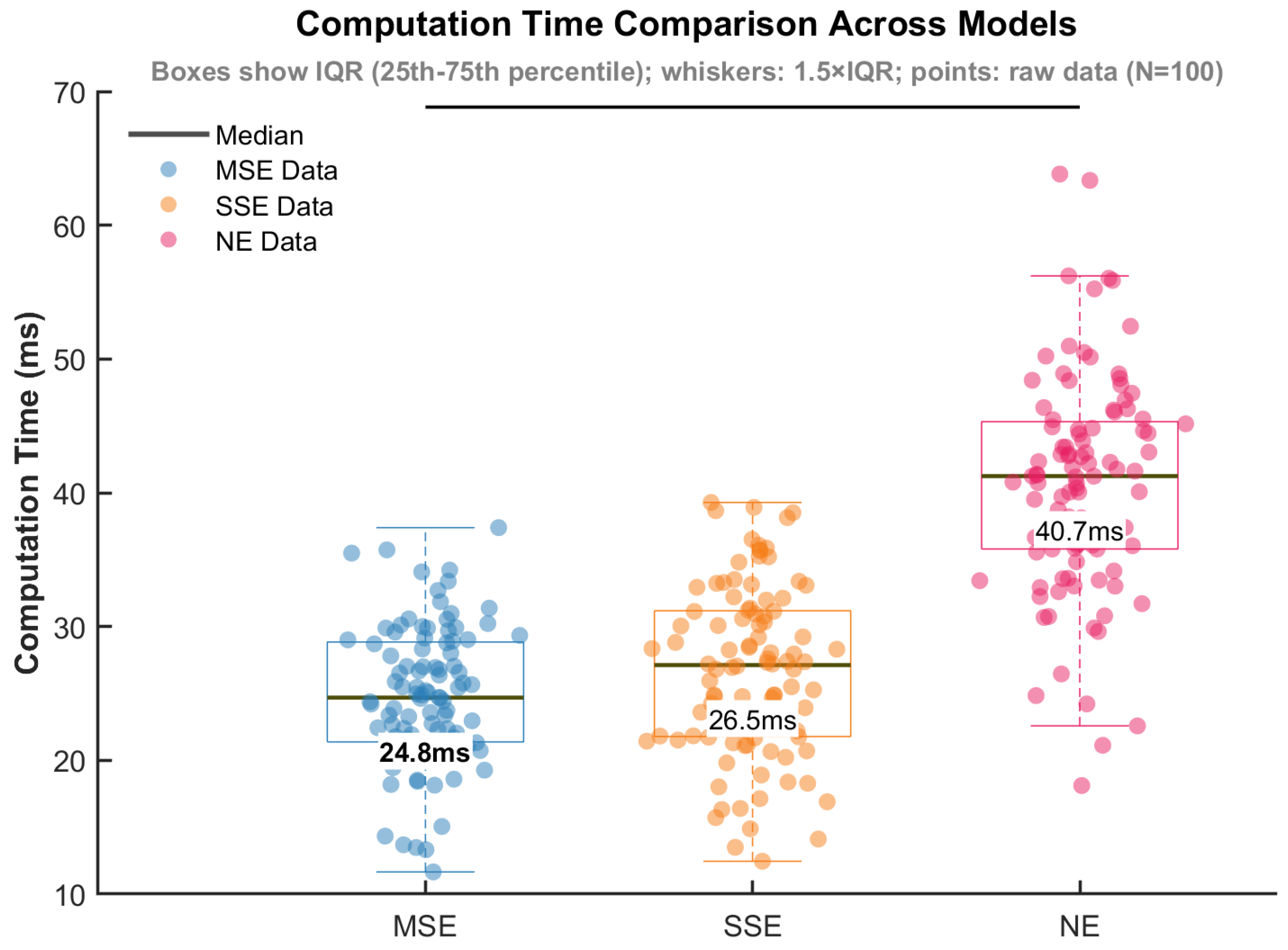
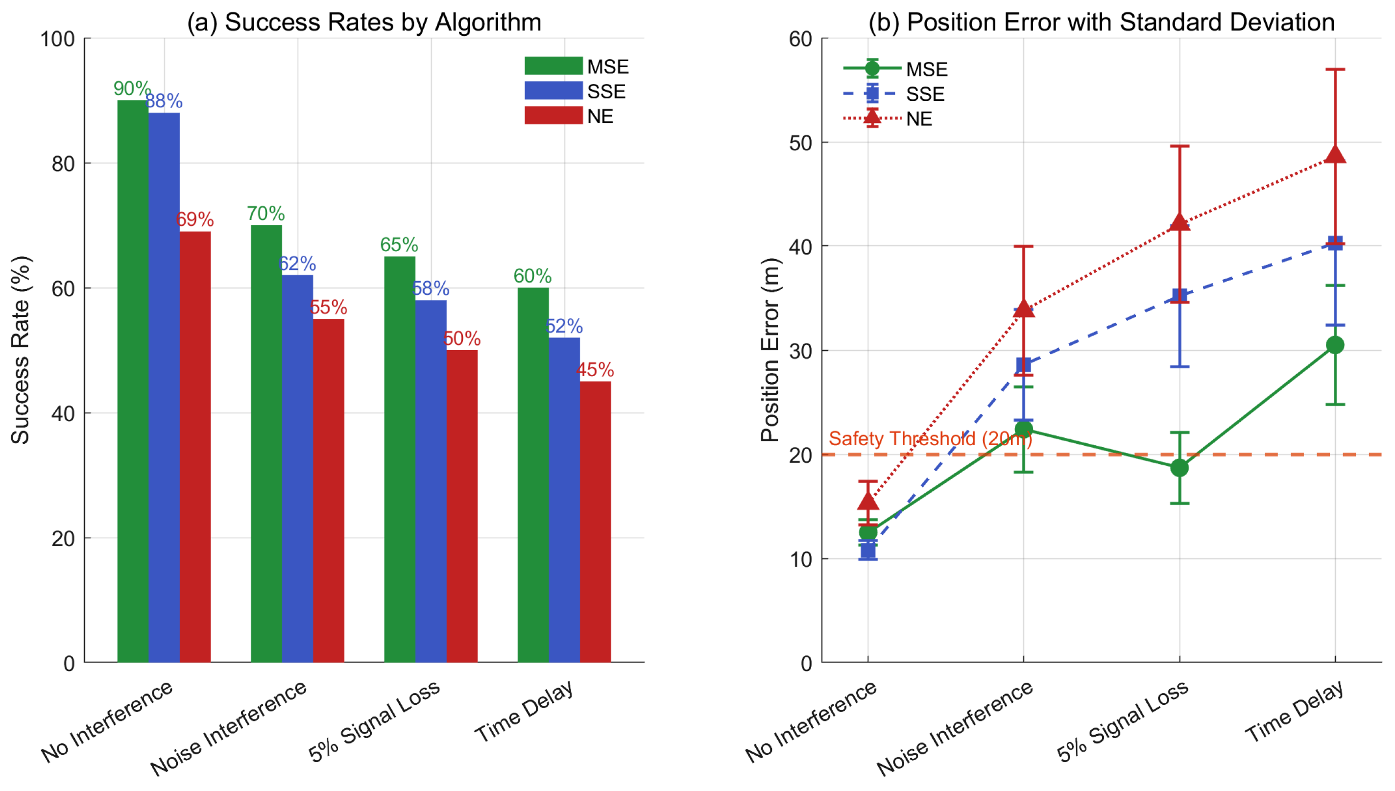
The existence and uniqueness of the solution to the Stackelberg game model are rigorously proven. Furthermore, the proposed MSE algorithm is compared with traditional methods, such as Nash Equilibrium (NE) [18] and Single–step Prediction Stackelberg Equilibrium (SSE) [24]. Numerical simulations demonstrate that the MSE algorithm offers significant advantages in terms of computational efficiency (e.g., an average generation time of 24.79 ms, which is 7.36% less than SSE and 39.11% less than NE), fuel consumption, pursuit success rate, and disturbance rejection capability.

3.

While Stackelberg games have been applied to spacecraft PE problems, this work lies in unifying Riccati–based Stackelberg solutions with model reference adaptive control, addressing $J_2$ perturbations and incomplete information—a gap in prior work.

The remainder of this article is organized as follows. In Section 2, the spacecraft PE game model is introduced and mapped onto a Stackelberg equilibrium system. In Section 3, the MSE tracking control method is proposed. Subsequently, Section 4 conducts simulation experiments. Finally, Section 5 summarizes the article.

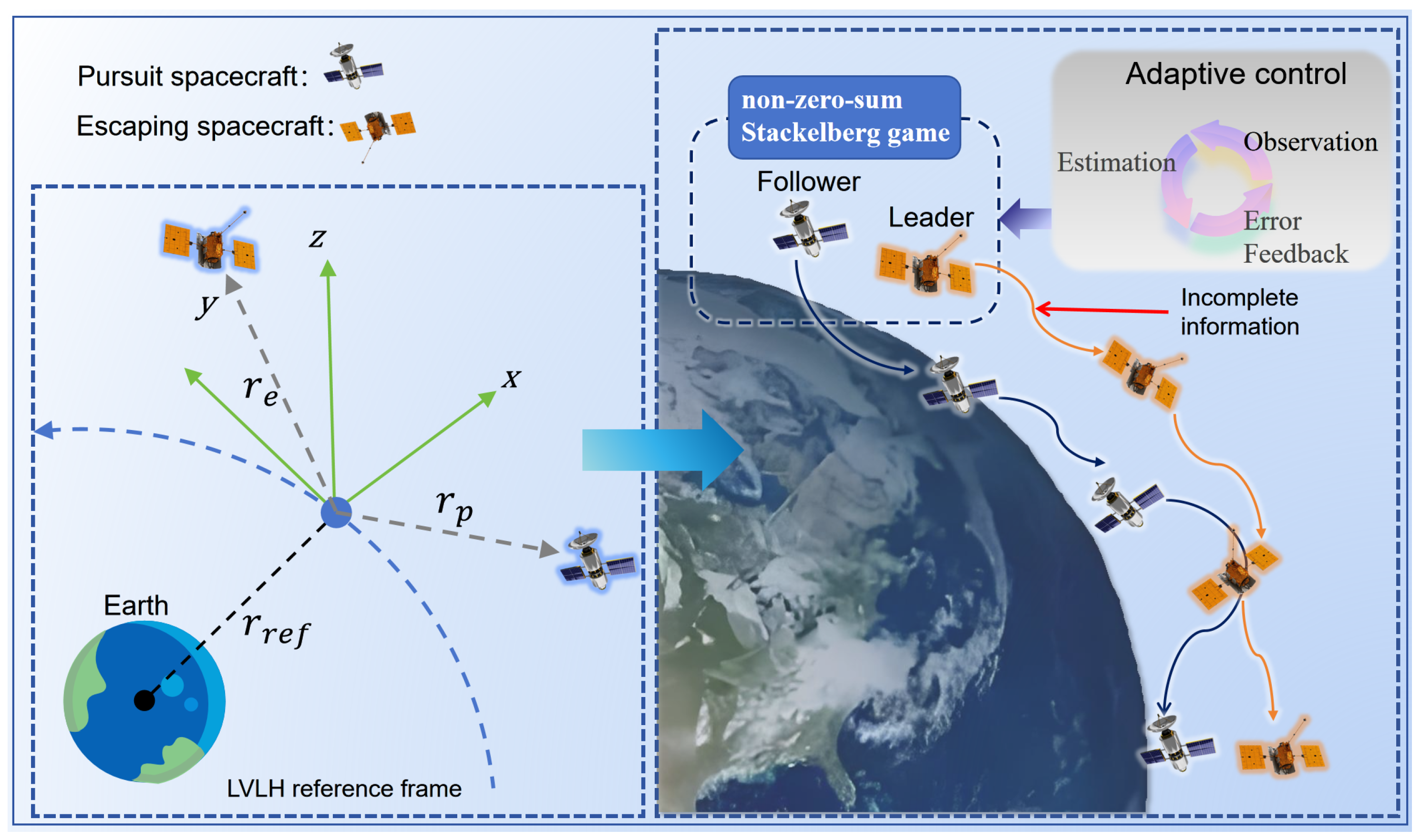
2. Problem Formulation

2.1. System Model

In spacecraft PE games, the relative dynamics equations of the spacecraft are described in the Local Vertical Local Horizontal (LVLH) coordinate system, as illustrated in Figure 1. The LVLH frame is centered on a virtual reference spacecraft following a nominal reference orbit. The x-axis points from the Earth’s center toward the origin, the y-axis lies within the orbital plane, perpendicular to the x-axis and aligned with the direction of the spacecraft’s motion, while the z-axis is determined by the right–hand rule, coinciding with the direction of the orbital angular momentum.

The dynamics of a single spacecraft in the Local Vertical Local Horizontal (LVLH) coordinate system can be described as follows [24]:

$$\left\{\begin{array}{c}\ddot{x}-2n_c\dot{y}-(5c^2-2)n^{2}x=-3n^2{J}_2{\left({\displaystyle \frac{R_e}{r_{ref}}}\right)}^2\times \left\{{\displaystyle \frac{1}{2}}-A-B\right\}+a_x\hfill \\ \ddot{y}+2n_c\dot{x}=-3n^2{J}_2{\left({\displaystyle \frac{R_e}{r_{ref}}}\right)}^2{sin}^2\left(i_{ref}\right)sin\left(kt\right)cos\left(kt\right)+a_y\hfill \\ \ddot{z}+q^{2}z=2lqcos(qt+\varphi )+a_z\hfill \end{array}\right.$$

(1)

These equations represent the relative motion in the LVLH frame, including the primary effects of the Earth’s oblateness ($J_2$ perturbation). The terms involving $n^2$ describe linearized gravitational and centrifugal forces, while the terms with $2n_c$ represent Coriolis forces. The $J_2$ perturbation introduces additional forces that cause long–term drift, which are captured by the trigonometric terms and constants defined in Appendix A. We denote the state and control input for the pursuer as ${\mathit{f}}_p$ and ${\mathit{a}}_p$, and for the evader as ${\mathit{f}}_e$ and ${\mathit{a}}_e$, respectively. The control inputs ${\mathit{a}}_p,{\mathit{a}}_e\in {\mathbb{R}}^3$ represent the thrust acceleration vectors. The relative state of the PE game is defined as $\tilde{\mathit{f}}={\mathit{f}}_e-{\mathit{f}}_p$. After feedback linearization and discretization, the relative dynamics of the PE game can be expressed as:

$${\tilde{\mathit{f}}}_{t+1}={\mathit{X}}_d{\tilde{\mathit{f}}}_t+{\mathit{Y}}_d{\mathit{a}}_{p,t+1}+{\mathit{Y}}_e{\mathit{a}}_{e,t}$$

(2)

The state vector ${\tilde{\mathit{f}}}_t\in {\mathbb{R}}^6$ and control inputs ${\mathit{a}}_{p,t},{\mathit{a}}_{e,t}\in {\mathbb{R}}^3$ imply that the control gain matrices ${\mathit{L}}_{p,t},{\mathit{L}}_{e,t}$ map ${\mathbb{R}}^6\to {\mathbb{R}}^3$; hence, their dimensions are $3\times 6$. The adaptive gain matrices ${\mathbf{\Gamma }}_p,{\mathbf{\Gamma }}_e\in {\mathbb{R}}^{6\times 6}$ are positive definite to ensure compatibility with the state–space update laws (Equation (28)). The system matrices ${\mathit{X}}_d,{\mathit{Y}}_d,{\mathit{Y}}_e$ are derived from the continuous–time dynamics.

2.2. Dynamic Stackelberg Pursuit–Evasion Game

In the spacecraft PE problem, the evader acts as the leader in a Stackelberg game, and the pursuer is the follower. In this Stackelberg game, the information structure is sequential and asymmetric. The leader (evader) commits to a strategy first. The follower (pursuer) observes the leader’s action and then chooses its own strategy to optimize its objective function. This does not imply direct real–time communication of the entire strategy, but rather that the pursuer’s decision–making process at time t is based on knowledge of the evader’s action at time t. The decision–making process is modeled as a dynamic game where each player optimizes a cost function. The cost functions for the pursuer (${\mathit{J}}_p$) and evader (${\mathit{J}}_e$) are defined as:

$${\mathit{J}}_p({\tilde{\mathit{f}}}_0,{\mathit{a}}_{p,t},{\mathit{a}}_{e,t})=\sum _{t=0}^{N-1}\{{\tilde{\mathit{f}}}_t^{\mathrm{T}}{\mathit{V}}_p{\tilde{\mathit{f}}}_t+{\mathit{a}}_{p,t}^{\mathrm{T}}{\mathit{W}}_{1,p}{\mathit{a}}_{p,t}-{\mathit{a}}_{e,t}^{\mathrm{T}}{\mathit{W}}_{1,e}{\mathit{a}}_{e,t}\}+{\tilde{\mathit{f}}}_N^{\mathrm{T}}{\mathit{V}}_{N,p}{\tilde{\mathit{f}}}_N$$

(3)

In this equation, ${\mathit{V}}_P$ and ${\mathit{V}}_{N,P}$ are 6 × 6 positive definite weighting matrices for the relative state error, while ${\mathit{W}}_{1,P}$ and ${\mathit{W}}_{1,e}$ are 3 × 3 positive definite weighting matrices for the control effort of the pursuer and evader, respectively. These matrices are design parameters used to tune the controller’s performance.

$${\mathit{J}}_e({\tilde{\mathit{f}}}_0,{\mathit{a}}_{p,t},{\mathit{a}}_{e,t})=-\sum _{t=0}^{N-1}\{{\tilde{\mathit{f}}}_t^{\mathrm{T}}{\mathit{V}}_e{\tilde{\mathit{f}}}_t+{\mathit{a}}_{p,t}^{\mathrm{T}}{\mathit{W}}_{2,p}{\mathit{a}}_{p,t}-{\mathit{a}}_{e,t}^{\mathrm{T}}{\mathit{W}}_{2,e}{\mathit{a}}_{e,t}\}-{\tilde{\mathit{f}}}_N^{\mathrm{T}}{\mathit{V}}_{N,e}{\tilde{\mathit{f}}}_N$$

(4)

Here, ${\mathit{V}}_e$,${\mathit{V}}_{N,e}$,${\mathit{W}}_{2,p}$, and ${\mathit{W}}_{2,e}$ are similarly defined positive definite weighting matrices.

A Stackelberg equilibrium is a pair of strategies (${\mathit{a}}_{p,t}^{*}$,${\mathit{a}}_{e,t}^{*}$) that satisfies:

$$\begin{array}{c}{\mathit{J}}_e\left({\tilde{\mathit{f}}}_0,{\mathit{a}}_{p,t}^{*},{\mathit{a}}_{e,t}^{*}\right)\le {\mathit{J}}_e\left({\tilde{\mathit{f}}}_0,{\mathit{a}}_{p,t}^{*},{\mathit{a}}_{e,t}\right)\\ {\mathit{J}}_p\left({\tilde{\mathit{f}}}_0,{\mathit{a}}_{p,t}^{*},{\mathit{a}}_{e,t}^{*}\right)\le {\mathit{J}}_p\left({\tilde{\mathit{f}}}_0,{\mathit{a}}_{p,t},{\mathit{a}}_{e,t}^{*}\right)\end{array}$$

(5)

It is important to distinguish the Stackelberg equilibrium condition in (5) from Pontryagin’s Minimum Principle (PMP). PMP provides necessary conditions for a single control to be optimal for a given objective function. In contrast, a Stackelberg Equilibrium is a solution concept for a bi–level game, defining a pair of strategies $({\mathit{a}}_p^{*},{\mathit{a}}_e^{*})$ where neither player has an incentive to unilaterally deviate, given the hierarchical decision structure.

We model this dynamic interaction as the following two–stage Stackelberg optimization problem:

$$\begin{array}{c}\underset{a_{e,t}}{min}{\mathit{J}}_e({\tilde{\mathit{f}}}_0,{\mathit{a}}_{p,t}^{*}\left({\mathit{a}}_{e,t}\right),{\mathit{a}}_{e,t})\\ \mathrm{s}.\mathrm{t}.{\mathit{a}}_{p,t}^{*}\left({\mathit{a}}_{e,t}\right)=arg\underset{{\mathit{a}}_{p,t}}{min}{\mathit{J}}_p({\tilde{\mathit{f}}}_0,{\mathit{a}}_{p,t},{\mathit{a}}_{e,t})\\ \mathrm{and}{\tilde{\mathit{f}}}_{t+1}={\mathit{X}}_d{\tilde{\mathit{f}}}_t+{\mathit{Y}}_e({\mathit{a}}_{e,t}-{\mathit{a}}_{p,t})\end{array}$$

(6)

The hierarchical structure of the minimization problem itself acts as the primary constraint embodying the Stackelberg game logic; the inner minimization of ${\mathit{J}}_p$ with respect to ${\mathit{a}}_{p,t}$ is solved first for a given ${\mathit{a}}_{e,t}$, yielding an optimal response function for the pursuer, ${\mathit{a}}_{p,t}^{*}\left({\mathit{a}}_{e,t}\right)$. The outer minimization of ${\mathit{J}}_e$ is then solved by the leader (evader), who anticipates the follower’s rational response. The system dynamics in (2) serve as a hard constraint that both players must adhere to.

3. Stackelberg Equilibrium–Based Model Reference Adaptive Control Algorithm

3.1. Resolution of Stackelberg Game

The Stackelberg PE game formulated in (6) is a bi–level, constrained optimization problem, where the system dynamics (2) serve as a hard constraint. To solve this, we first transform it into an unconstrained problem by incorporating the dynamics into the cost functions using a set of positive definite matrices ${\mathit{P}}_{p,t}$ and ${\mathit{P}}_{e,t}$. The derivation of the optimal control laws via the coupled Riccati Equations (7) and (8) relies on standard assumptions in optimal control theory. Specifically, for a solution to exist, the system dynamics matrix pairs must be stabilizable, and the weighting matrices in the cost functions are chosen to be positive definite, which ensures the convexity of the optimization problem. This transformation leads to an unconstrained optimization problem with the cost functions (3) and (4). Based on these, the Stackelberg PE control strategy is designed. For the pursuer’s (follower’s) cost function ${\mathit{J}}_p$, the follower makes its decision ${\mathit{a}}_{p,t}$ after observing the leader’s (evader’s) action ${\mathit{a}}_{e,t}^{*}$. Therefore, to find the pursuer’s optimal strategy, we substitute the system dynamics (2) into the summation term ${\mathit{F}}_{p,t}$. The optimal linear control strategy is of the form ${\mathit{a}}_{p,t}={\mathit{L}}_{p,t}{\tilde{\mathit{f}}}_t$ and ${\mathit{a}}_{e,t}={\mathit{L}}_{e,t}{\tilde{\mathit{f}}}_t$. The control gain matrices ${\mathit{L}}_{p,t}$ and ${\mathit{L}}_{e,t}$ are of dimension 3 × 6, mapping the state space ${\mathbb{R}}^6$ to control input space ${\mathbb{R}}^3$. By minimizing the respective cost functions, we arrive at a set of coupled discrete–time Riccati equations. For the evader (leader), the Riccati equation is:

$$\begin{array}{c}{\mathit{P}}_{e,t}={\mathit{L}}_{e,t}^{*\mathrm{T}}\left({\mathit{W}}_{2,e}-{\mathit{Y}}_e^{\mathrm{T}}{\mathit{P}}_{e,t+1}{\mathit{Y}}_e\right){\mathit{L}}_{e,t}^{*}+{\mathit{L}}_{p,t}^{*\mathrm{T}}\left({\mathit{W}}_{2,p}+{\mathit{Y}}_p^{\mathrm{T}}{\mathit{P}}_{e,t+1}{\mathit{Y}}_p\right){\mathit{L}}_{p,t}^{*}+\hfill \\ \hfill {\mathit{V}}_e+{\mathit{X}}_d^{\mathrm{T}}{\mathit{P}}_{e,t+1}{\mathit{X}}_d+{\mathit{X}}_d^{\mathrm{T}}{\mathit{P}}_{e,t+1}{\mathit{Y}}_p{\mathit{L}}_{p,t}^{*}+{\mathit{L}}_{p,t}^{*\mathrm{T}}{\mathit{Y}}_p^{\mathrm{T}}{\mathit{P}}_{e,t+1}{\mathit{X}}_d\end{array}$$

(7)

The evader’s optimal strategy is derived via a Riccati equation, which encodes the cost trade–offs between state deviation and control effort. For the pursuer, the equation incorporates the evader’s anticipated actions, reflecting the hierarchical Stackelberg structure. For the pursuer (follower), the Riccati equation is:

$$\begin{array}{c}\hfill {\mathit{P}}_{p,t}=-{\mathit{L}}_{p,t}^{*\mathrm{T}}\left({\mathit{W}}_{1,p}+{\mathit{Y}}_p^{\mathrm{T}}{\mathit{P}}_{p,t+1}{\mathit{Y}}_p\right){\mathit{L}}_{p,t}^{*}+{\mathit{L}}_{e,t}^{*\mathrm{T}}\left({\mathit{Y}}_e^{\mathrm{T}}{\mathit{P}}_{p,t+1}{\mathit{Y}}_e-{\mathit{W}}_{1,p}\right){\mathit{L}}_{e,t}^{*}+\\ {\mathit{V}}_p+{\mathit{X}}_d^{\mathrm{T}}{\mathit{P}}_{p,t+1}{\mathit{X}}_d+{\mathit{X}}_d^{\mathrm{T}}{\mathit{P}}_{p,t+1}{\mathit{Y}}_e{\mathit{L}}_{e,t}^{*}+{\mathit{L}}_{e,t}^{*}{\mathit{Y}}_e^{\mathrm{T}}{\mathit{P}}_{e,t+1}{\mathit{X}}_d\hfill \end{array}$$

(8)

These Riccati equations are solved backward in time, starting from the terminal boundary conditions ${\mathit{P}}_{p,N}={\mathit{V}}_{N,p}$ and ${\mathit{P}}_{e,N}={\mathit{V}}_{N,e}$, which are the terminal cost matrices from (3) and (4).

To provide a unified expression, we introduce the coupling matrix ${\mathit{\psi }}_t$, defined as:

$${\mathit{\psi }}_t=\left[\begin{array}{cc}{\mathit{W}}_{1,p}+{\mathit{Y}}_p^{\mathrm{T}}{\mathit{P}}_{p,t+1}{\mathit{Y}}_p& {\mathit{Y}}_p^{\mathrm{T}}{\mathit{P}}_{p,t+1}{\mathit{Y}}_e\\ -{\mathit{Y}}_e^{\mathrm{T}}{\mathit{P}}_{e,t+1}{\mathit{Y}}_p& {\mathit{W}}_{2,e}-{\mathit{Y}}_e^{\mathrm{T}}{\mathit{P}}_{e,t+1}{\mathit{Y}}_e\end{array}\right]$$

(9)

The optimal control gain vector ${\mathit{L}}_t^{*}={\left[\begin{array}{cc}{\mathit{L}}_{p,t}^{*}& {\mathit{L}}_{e,t}^{*}\end{array}\right]}^{\mathrm{T}}$ can then be solved for simultaneously:

$${\mathit{L}}_t^{*}={\mathbf{\Psi }}_t^{-1}\left[\begin{array}{c}-{\mathit{Y}}_p^{\mathrm{T}}{\mathit{P}}_{p,t+1}{\mathit{X}}_d\\ {\mathit{Y}}_e^{\mathrm{T}}{\mathit{P}}_{e,t+1}{\mathit{X}}_d\end{array}\right]$$

(10)

Mathematically, a Nash Equilibrium solves a set of simultaneous optimization problems: ${\mathit{a}}_p^{*}=arg \underset{{\mathit{a}}_p}{min} {\mathit{J}}_p({\mathit{a}}_p^{*},{\mathit{a}}_e)$ and ${\mathit{a}}_e^{*}=arg \underset{{\mathit{a}}_e}{min} {\mathit{J}}_e({\mathit{a}}_p^{*},{\mathit{a}}_e)$. In contrast, the Stackelberg equilibrium solves the hierarchical problem shown in (6). This structural difference, captured by the coupled Riccati Equations (7) and (8) and the resulting asymmetric gain solution in (10), avoids the unrealistic assumption of simultaneous moves inherent in Nash models. In terms of computational complexity, the main burden is solving the N–coupled Riccati equations, which scales linearly with the horizon N. Each step involves matrix multiplications and an inversion of the $6\times 6$ coupling matrix ${\mathbf{\Psi }}_t$, which has a constant complexity. The online adaptive update is computationally light.

3.2. Existence and Uniqueness of Stackelberg Equilibria

For a unique Stackelberg equilibrium to exist, the following conditions must be met [25]:

1.

The strategy sets for the leader and follower are non–empty compact convex sets.

2.

For a given leader’s strategy, a unique optimal solution for the follower exists.

3.

For a given follower’s strategy, a unique optimal solution for the leader exists.

We now verify that these three conditions are met:

1.

(Non–empty compact convex set): The strategy spaces are subsets of Euclidean space and are non–empty. The cost functions (3) and (4) are quadratic, and thus continuous, with respect to the control actions. As ${\mathit{J}}_p$ and ${\mathit{J}}_e$ are strictly convex and tend to infinity as the norms of the control actions approach infinity, this ensures the existence of a minimum and that the set of optimal strategies is compact and convex.

2.

(Unique follower solution): For any given leader’s strategy ${\mathit{a}}_{e,t}$, the follower’s (pursuer’s) cost function ${\mathit{J}}_p$ in (4) is strictly convex in ${\mathit{a}}_{p,t}$. Strict convexity is guaranteed because its quadratic weighting matrix, $({\mathit{W}}_{1,p}+{\mathit{Y}}_p^T{\mathit{P}}_{p,t+1}{\mathit{Y}}_p)$, is positive definite. This holds because ${\mathit{W}}_{1,p}$ is chosen as positive definite, and ${\mathit{P}}_{p,t+1}$, as a solution to the Riccati equation, is also positive definite, making ${\mathit{Y}}_p^T{\mathit{P}}_{p,t+1}{\mathit{Y}}_p$ positive semi–definite. A strictly convex function has a unique minimum.

3.

(Unique leader solution): Similarly, when the follower’s strategy is given, the leader’s (evader’s) cost function ${\mathit{J}}_e$ in (3) is strictly convex in ${\mathit{a}}_{e,t}$, as ${\mathit{W}}_{2,e}{\mathit{Y}}_{e,t+1}{\mathit{Y}}_e$ is designed to be positive definite. This guarantees a unique optimal solution for the leader.

Furthermore, the uniqueness of the solution is guaranteed by the invertibility of the coupling matrix ${\mathit{\psi }}_t$ in Equation (10), which is ensured by the conditions above.

3.3. Stackelberg Equilibrium–Based Model Reference Adaptive Control Algorithm

After obtaining the optimal control strategy of the evader in the Stackelberg game, ${\mathit{L}}_e^{*}$, we design a model reference adaptive controller for the pursuer. The controller uses the evader’s optimal strategy as a reference, allowing the pursuer to dynamically adjust its own controller parameters via observation and feedback to minimize error and achieve an efficient pursuit.

The adaptive update law for the pursuer’s estimate of the evader’s gain, ${\widehat{\mathit{L}}}_{e,m}$, is designed as a robust gradient–descent–type law derived from the estimation error dynamics.

$${\widehat{\mathit{L}}}_{e,m+1}={\widehat{\mathit{L}}}_{e,m}-fal\left({\mathit{\epsilon }}_t^m\right){\tilde{\mathit{f}}}_t^{\mathsf{T}}\Gamma (M+{\tilde{\mathit{f}}}_t^{\mathsf{T}}{\tilde{\mathit{f}}}_t{)}^{-1}$$

(11)

where ${ϵ}_t^m$ is the estimation error. The nonlinear function $fal(·)$ is used in place of a linear error term to achieve better performance. It provides high gain when the error is small, leading to faster convergence, and avoids excessive gain when the error is large, which enhances robustness to noise. It is defined as:

$$fal\left(x\right)={\left|x\right|}^{\tau }·sign\left(x\right)·\theta \left(\right|x|-\delta )+{\displaystyle \frac{x}{{\delta }^{1-\tau }}}·(1-\theta (\left|x\right|-\delta \left)\right)$$

(12)

Once the pursuer obtains a converged estimate of the evader’s gain, ${\widehat{\mathit{L}}}_e$, it calculates its own optimal control gain using:

$${\mathit{L}}_p^{*}=-{\left({\mathit{W}}_{1,p}+{\mathit{Y}}_p^{\mathsf{T}}{\widehat{\mathit{P}}}_p^{*}{\mathit{Y}}_p\right)}^{-1}{\mathit{Y}}_p^{\mathsf{T}}{\widehat{\mathit{P}}}_p^{*}\left({\mathit{X}}_d+{\mathit{Y}}_e{\widehat{\mathit{L}}}_e^{*}\right)$$

(13)

The stability of this adaptive system is proven using a Lyapunov–based analysis. By selecting an appropriate Lyapunov function candidate and designing the parameter update laws, it can be shown that the tracking and parameter estimation errors are uniformly ultimately bounded.

The overall control architecture is depicted in the flowchart in Figure 2, and a timeline of the process is shown in Figure 3.

Figure 2 illustrates the overall control architecture. The process is divided into two main parts: the Model Reference Part and the Adaptive Control Part. In the Model Reference Part (top), the system calculates the optimal reference gain for the evader, ${\mathit{L}}_e^{*}$. This involves initializing parameters, building the mathematical model, and iteratively solving the Riccati Equations (7) and (8) to compute the optimal strategies. The resulting optimal evader gain ${\mathit{L}}_e^{*}$ is then fed as a reference to the Adaptive Control Part (bottom). Here, the pursuer observes the system state and uses an adaptive law to update its own strategy ${\mathit{L}}_p^{*}$ to effectively track the evader’s behavior.

Figure 3 provides a timeline perspective of a single iteration cycle of the pursuer’s adaptive strategy generation. It begins with the ‘Pursuer Observation and Estimation’ phase, where the pursuer acquires the state of the evader. This is followed by ‘Error Feedback and Optimization’, where the error is calculated and parameters are updated based on the reference model. This leads to ‘Adaptive Strategy Generation’ and finally ‘Strategy execution and closure’. The cycle repeats, allowing for continuous adaptation.

Theorem 1.

Under assumptions 1–7, the following laws apply [25]:

1. 

The system dynamics (2) are Lipschitz continuous with respect to state and parameter variations, i.e., there exists ${\mathit{L}}_f>0$ such that:

$$∥\mathit{f}(x_1,{\mathit{L}}_1)-\mathit{f}(x_2,{\mathit{L}}_2)∥\le {\mathit{L}}_f(∥x_1-x_2∥+∥{\mathit{L}}_1-{\mathit{L}}_2∥)$$

(14)

2. 

The reference signal

$$∥{\widehat{\mathit{f}}}_t∥\le F_{max},∥{\dot{\widehat{\mathit{f}}}}_t∥\le G_{max}(\forall t\ge 0)$$

(15)

3. 

The disturbance $d_t$ is $L_{\infty }$–bounded with known upper bound:

$$∥{\mathit{d}}_t∥\le {\mathit{d}}_{max}\left(\forall t\ge 0\right)$$

(16)

4. 

There exist constants $\alpha >0$ and $T>0$ such that the regressor vector

$${\displaystyle \frac{1}{T}}{\int }_t^{t+T}{\widehat{\mathit{f}}}_{\tau }{\widehat{\mathit{f}}}_{\tau }^{\mathrm{T}}d\tau \ge \alpha \mathit{I}\forall t\ge 0$$

(17)

5. 

The initial parameter estimation errors satisfy:

$$∥{\tilde{\mathit{L}}}_{p,0}∥\le {\mathrm{\Delta }}_p,∥{\tilde{\mathit{L}}}_{e,0}∥\le {\mathrm{\Delta }}_e$$

(18)

6. 

The matrix ${\mathit{Y}}_e^T{\mathit{Y}}_e$ is uniformly positive definite, i.e., there exists ${\sigma }_{min}$ such that:

$${\lambda }_{min}\left({\mathit{Y}}_e^T{\mathit{Y}}_e\right)\ge {\sigma }_{min}$$

(19)

7. 

The adaptive gain matrices ${\mathbf{\Gamma }}_p,{\mathbf{\Gamma }}_e\in {\mathbb{R}}^{6\times 6}$ are symmetric positive definite, with eigenvalues bounded by:

$${\lambda }_{max}\left({\mathbf{\Gamma }}_{\mathit{p}}\right)\le {\displaystyle \frac{c_1}{{\gamma }_p{F}_{max}^2}},{\lambda }_{max}\left({\mathbf{\Gamma }}_{\mathit{e}}\right)\le {\displaystyle \frac{c_1}{{\gamma }_e{F}_{max}^2}}$$

(20)

and the higher–order term (h.o.t.) coefficient satisfies:

$$c_2=max\left({\gamma }_p{F}_{max}^2,{\gamma }_e{F}_{max}^2\right)$$

(21)

where $c_1,{\gamma }_p,{\gamma }_e>0$ are design constants.

Proof of Theorem 1.

Based on the assumption of system observability, according to (2), the control gain estimator is designed as follows:

$${\widehat{\mathit{f}}}_{t+1}^m={\mathit{Y}}_e{\widehat{\mathit{L}}}_{e,t}{\tilde{\mathit{f}}}_t+{\mathit{X}}_d{\tilde{\mathit{f}}}_t+{\mathit{Y}}_p{\mathit{a}}_{p,t}$$

(22)

where ${\widehat{\mathit{f}}}_{t+1}^m\in \mathbb{R}$ denotes the predicted state vector, ${\widehat{\mathit{L}}}_{e,t}\in {\mathbb{R}}^{m\times n}$ are the estimates of the relative state, ${\mathit{Y}}_e\in {\mathbb{R}}^{m\times n}$ is the known input coupling matrix. The true system dynamics follow:

$${\widehat{\mathit{f}}}_{t+1}={\mathit{X}}_d{\widehat{\mathit{f}}}_t+{\mathit{Y}}_e{\mathit{L}}_e^{*}{\widehat{\mathit{f}}}_t+{\mathit{Y}}_p{\mathit{a}}_{p,t+1}+{\mathit{d}}_t$$

(23)

with ${\mathit{L}}_e^{*}$ being the ideal (unknown) parameter matrix and ${\mathit{d}}_t$ accounting for bounded disturbances. The prediction error yields:

$${\mathit{\epsilon }}_t={\left({\mathit{Y}}_e^{\mathrm{T}}{\mathit{Y}}_e\right)}^{-1}{\mathit{Y}}_e^{\mathrm{T}}({\widehat{\mathit{f}}}_{t+1}^m-{\widehat{\mathit{f}}}_{t+1})=({\widehat{\mathit{L}}}_{e,t}-{\mathit{L}}_e^{*}){\widehat{\mathit{f}}}_t$$

(24)

The tracking error dynamics are governed by:

$${\mathit{e}}_{t+1}={\mathit{A}}_d{\mathit{e}}_t+{\mathit{Y}}_d{\tilde{\mathit{L}}}_{p,t}{\widehat{\mathit{f}}}_t-{\mathit{Y}}_e{\tilde{\mathit{L}}}_{e,t}{\widehat{\mathit{f}}}_t+{\mathit{d}}_t$$

(25)

where ${\mathit{A}}_d={\mathit{X}}_d+{\mathit{Y}}_d{\mathit{L}}_p^{*}-{\mathit{Y}}_e{\mathit{L}}_e^{*}$ is the ideal closed-loop matrix, ${\tilde{\mathit{L}}}_{p,t}={\widehat{\mathit{L}}}_{p,t}-{\mathit{L}}_p^{*}$ and ${\tilde{\mathit{L}}}_{e,t}={\widehat{\mathit{L}}}_{e,t}-{\mathit{L}}_e^{*}$ are parameter estimation errors. Consider the Lyapunov function candidate:

$${\mathit{V}}_t={\mathit{e}}_t^{\mathrm{T}}\mathit{P}{\mathit{e}}_t+\mathrm{tr}\left({\tilde{\mathit{L}}}_{p,t}^{\mathrm{T}}{\mathbf{\Gamma }}_p^{-1}{\tilde{\mathit{L}}}_{p,t}\right)+\mathrm{tr}\left({\tilde{\mathit{L}}}_{e,t}^{\mathrm{T}}{\mathbf{\Gamma }}_e^{-1}{\tilde{\mathit{L}}}_{e,t}\right)$$

(26)

where $\mathit{P}>0$ satisfies the discrete–time algebraic Riccati equation (DARE):

$${\mathit{A}}_d^{\mathrm{T}}\mathit{P}{\mathit{A}}_d-\mathit{P}=-\mathit{Q}$$

(27)

The parameter update law is designed as:

$${\widehat{\mathit{L}}}_{e,t+1}={\widehat{\mathit{L}}}_{e,t}-{\mathbf{\Gamma }}_e{\mathit{\epsilon }}_t{\widehat{\mathit{f}}}_t^{\mathsf{T}}{(M+{∥{\widehat{\mathit{f}}}_t∥}^2)}^{-1}$$

(28)

with ${\mathbf{\Gamma }}_p>0,{\mathbf{\Gamma }}_e>0$ being symmetric positive definite learning rate matrices. The Lyapunov difference must be meticulously expanded as follows:

$$\begin{array}{c}\mathrm{\Delta }{\mathit{V}}_{1,t}={\mathit{e}}_{t+1}^{\mathrm{T}}\mathit{P}{\mathit{e}}_{t+1}-{\mathit{e}}_t^{\mathrm{T}}\mathit{P}{\mathit{e}}_t\hfill \\ \mathrm{\Delta }{\mathit{V}}_{2,t}=\mathrm{tr}({\tilde{\mathit{L}}}_{p,t+1}^{\mathrm{T}}{\mathbf{\Gamma }}_p^{-1}{\tilde{\mathit{L}}}_{p,t+1}-{\tilde{\mathit{L}}}_{p,t}^{\mathrm{T}}{\mathbf{\Gamma }}_p^{-1}{\tilde{\mathit{L}}}_{p,t})\hfill \\ \mathrm{\Delta }{\mathit{V}}_{3,t}=\mathrm{tr}({\tilde{\mathit{L}}}_{e,t+1}^{\mathrm{T}}{\mathbf{\Gamma }}_e^{-1}{\tilde{\mathit{L}}}_{e,t+1}-{\tilde{\mathit{L}}}_{e,t}^{\mathrm{T}}{\mathbf{\Gamma }}_e^{-1}{\tilde{\mathit{L}}}_{e,t})\hfill \end{array}$$

Substituting the error dynamics (25), we derive:

$$\mathrm{\Delta }{\mathit{V}}_{1,t}={\mathit{e}}_t^{\mathrm{T}}({\mathit{A}}_d^{\mathrm{T}}\mathit{P}{\mathit{A}}_d-\mathit{P}){\mathit{e}}_t+2{\mathit{e}}_t^{\mathrm{T}}{\mathit{A}}_d^{\mathrm{T}}\mathit{P}({\mathit{Y}}_d{\tilde{\mathit{L}}}_{p,t}-{\mathit{Y}}_e{\tilde{\mathit{L}}}_{e,t}){\widehat{\mathit{f}}}_t+\mathcal{O}\left({∥\tilde{\mathit{L}}∥}^2\right)$$

(29)

Using the DARE, this simplifies to:

$$\mathrm{\Delta }{\mathit{V}}_{1,t}=-{\mathit{e}}_t^{\mathrm{T}}\mathit{Q}{\mathit{e}}_t+2{\mathit{e}}_t^{\mathrm{T}}{\mathit{A}}_d^{\mathrm{T}}\mathit{P}({\mathit{Y}}_d{\tilde{\mathit{L}}}_{p,t}-{\mathit{Y}}_e{\tilde{\mathit{L}}}_{e,t}){\widehat{\mathit{f}}}_t+\mathrm{h}.\mathrm{o}.\mathrm{t}.$$

(30)

Assuming the parameter update laws:

$$\begin{array}{c}{\widehat{\mathit{L}}}_{p,t+1}={\widehat{\mathit{L}}}_{p,t}+{\mathbf{\Gamma }}_p{\mathit{Y}}_d^{\mathrm{T}}\mathit{P}{\mathit{e}}_t{\widehat{\mathit{f}}}_t^{\mathrm{T}}\hfill \\ {\widehat{\mathit{L}}}_{e,t+1}={\widehat{\mathit{L}}}_{e,t}-{\mathbf{\Gamma }}_e{\mathit{Y}}_e^{\mathrm{T}}\mathit{P}{\mathit{e}}_t{\widehat{\mathit{f}}}_t^{\mathrm{T}}\hfill \end{array}$$

(31)

the parameter error differences are:

$$\mathrm{\Delta }{\mathit{V}}_{2,t}+\mathrm{\Delta }{\mathit{V}}_{3,t}=2\mathrm{tr}\left({\tilde{\mathit{L}}}_{p,t}^{\mathrm{T}}{\mathit{Y}}_d^{\mathrm{T}}\mathit{P}{\mathit{e}}_t{\widehat{\mathit{f}}}_t^{\mathrm{T}}\right)-2\mathrm{tr}\left({\tilde{\mathit{L}}}_{e,t}^{\mathrm{T}}{\mathit{Y}}_e^{\mathrm{T}}\mathit{P}{\mathit{e}}_t{\widehat{\mathit{f}}}_t^{\mathrm{T}}\right)+\mathcal{O}\left({\mathbf{\Gamma }}^2\right)$$

(32)

Combining all terms yields:

$$\begin{array}{c}\mathrm{\Delta }{\mathit{V}}_t⩽-{\mathit{e}}_t^{\mathrm{T}}\mathit{Q}{\mathit{e}}_t+2{\mathit{e}}_t^{\mathrm{T}}({\mathit{A}}_d^{\mathrm{T}}\mathit{P}+\mathit{P})({\mathit{Y}}_d{\tilde{\mathit{L}}}_{p,t}-{\mathit{Y}}_e{\tilde{\mathit{L}}}_{e,t}){\widehat{\mathit{f}}}_t+\hfill \\ \hspace{1em}\hspace{1em}\gamma {∥{\widehat{\mathit{f}}}_t∥}^2({∥{\tilde{\mathit{L}}}_{p,t}∥}^2+{∥{\tilde{\mathit{L}}}_{e,t}∥}^2)\hfill \end{array}$$

(33)

By selecting sufficiently large $\mathit{Q}$ and appropriate learning rates $\mathbf{\Gamma }$, we ensure:

$$\mathrm{\Delta }{\mathit{V}}_t\le -c_1\parallel {\mathit{e}}_t{\parallel }^2+ c_2(\parallel {\tilde{\mathit{L}}}_{p,t}{\parallel }^2+ \parallel {\tilde{\mathit{L}}}_{e,t}{\parallel }^2)$$

(34)

Defining the estimation error

$${\mathit{\epsilon }}_t^m\stackrel{\mathrm{\Delta }}{=}{\left({\mathit{Y}}_e^{\mathsf{T}}{\mathit{Y}}_e\right)}^{-1}{\mathit{Y}}_e^{\mathsf{T}}({\widehat{\mathit{f}}}_{t+1}^m-{\tilde{\mathit{f}}}_{t+1})$$

(35)

then (35) can be written as  

$${\mathit{\epsilon }}_t^m=({\widehat{\mathit{L}}}_{e,m}-{\mathit{L}}_e^{*}){\tilde{\mathit{f}}}_t$$

(36)

According to (36), the design ${\widehat{\mathit{L}}}_{e,m}$ of the adaptive update rule is

$${\widehat{\mathit{L}}}_{e,m+1}={\widehat{\mathit{L}}}_{e,m}-\mathrm{fal}\left({ϵ}_t^m\right){\tilde{\mathit{f}}}_t^T\mathbf{\Gamma }{(M+{\tilde{\mathit{f}}}_t^T{\tilde{\mathit{f}}}_t)}^{-1}$$

(37)

where M denotes a constant value, while $\mathrm{\Gamma }$ represents a matrix that is positively definite, denoting a nonlinear function $fal(·)$

$$fal\left(x\right)={\left|x\right|}^{\tau }·sign\left(x\right)·\theta \left(\right|x|-\delta )+{\displaystyle \frac{x}{{\delta }^{1-\tau }}}·(1-\theta (\left|x\right|-\delta \left)\right)$$

(38)

where $x\in \mathbb{R},\delta ,\tau \in (0,1]$ is an adjustable parameter, $\theta$ denotes the unit step function, and $\left|x\right|-\delta$  is equal to 1 when $\left|x\right|-\delta$ is greater than 0, and 0 otherwise. When $∥{\widehat{\mathit{L}}}_{e,m+1}-{\widehat{\mathit{L}}}_{e,m}∥\le \kappa ∥{\widehat{\mathit{L}}}_{e,m}-{\widehat{\mathit{L}}}_{e,m-1}∥$ is satisfied, the controller sets ${\widehat{\mathit{L}}}_e^{*}\leftarrow {\widehat{\mathit{L}}}_{e,m+1}$, where $0<\kappa \le 1$ denotes the adjustable parameter. Equation (38) shows that $\mathrm{\Delta }{V}_t$ is negative as long as ${\left|e_t\right|}^2>(c_2/c_1)({\left|{\tilde{\mathit{L}}}_{p,t}\right|}^2+{\left|{\tilde{\mathit{L}}}_{e,t}\right|}^2)$. This does not guarantee asymptotic stability, but it does prove that the tracking error ${\mathit{e}}_t$ and parameter estimation errors ${\tilde{\mathit{L}}}_{p,t},{\tilde{\mathit{L}}}_{e,t}$ are uniformly ultimately bounded, as stated in Theorem 1. With the additional condition of Persistent Excitation (PE) on the regressor ${\widehat{\mathit{f}}}_t$, it can be further shown that the parameter errors converge, which in turn leads to the exponential convergence of the tracking error ${\mathit{e}}_t$ to a small neighborhood of the origin. When the persistent excitation condition (Equation (17)) is satisfied, the parameter error $∥{\tilde{\mathit{L}}}_{e,t}∥$ converges at an exponential rate, which in turn ensures that the tracking error ${\mathit{e}}_t$ converges at an exponential rate.    □

To consolidate the proposed method, Algorithm 1 provides a step–by–step procedure for implementation. The overall approach consists of an offline stage to compute the reference Stackelberg strategies and an online adaptive stage where the pursuer refines its strategy.

Algorithm 1 Stackelberg Equilibrium–Based Model Reference Adaptive Control

Require: System matrices as defined in (2)–(4); estimation threshold $\kappa >0$ Ensure: Optimal control strategies ${\mathit{L}}_p^{*}$ (pursuer) and ${\mathit{L}}_e^{*}$ (evader)   1: $t\Leftarrow 1$, $m\Leftarrow 1$   2: Initialize boundary conditions   3: for $t\Leftarrow 1$ to N do   4:     ${\mathit{\psi }}_t\Leftarrow \mathrm{Compute}\mathrm{via}$(9)   5:     if ${\mathit{\psi }}_t$ is invertible then   6:         ${\mathit{L}}_e^{*}\Leftarrow \mathrm{Solve}\mathrm{using}$(10)   7:         ${\mathit{P}}_{p,k},{\mathit{P}}_{e,k}\Leftarrow \mathrm{Update}\mathrm{via}$(7) and (8)   8:     end if   9: end for 10: for $m\Leftarrow 1$ to M do 11:     ${\epsilon }_t^m\Leftarrow \mathrm{Evaluate}\mathrm{from}$(36) 12:     ${\widehat{\mathit{L}}}_{e,m+1}\Leftarrow \mathrm{Refine}\mathrm{via}$(37) 13:     if $∥{\widehat{\mathit{L}}}_{e,m+1}-{\widehat{\mathit{L}}}_{e,m}∥\le \kappa ∥{\widehat{\mathit{L}}}_{e,m}-{\widehat{\mathit{L}}}_{e,m-1}∥$ then 14:         ${\mathit{L}}_e^{*}\Leftarrow {\widehat{\mathit{L}}}_{e,m+1}$ 15:         return ${\mathit{L}}_e^{*}$ 16:         break 17:     end if 18: end for 19: ${\mathit{L}}_p^{*}\Leftarrow \mathrm{Derive}\mathrm{from}$(13) 20: return  ${\mathit{L}}_p^{*}$

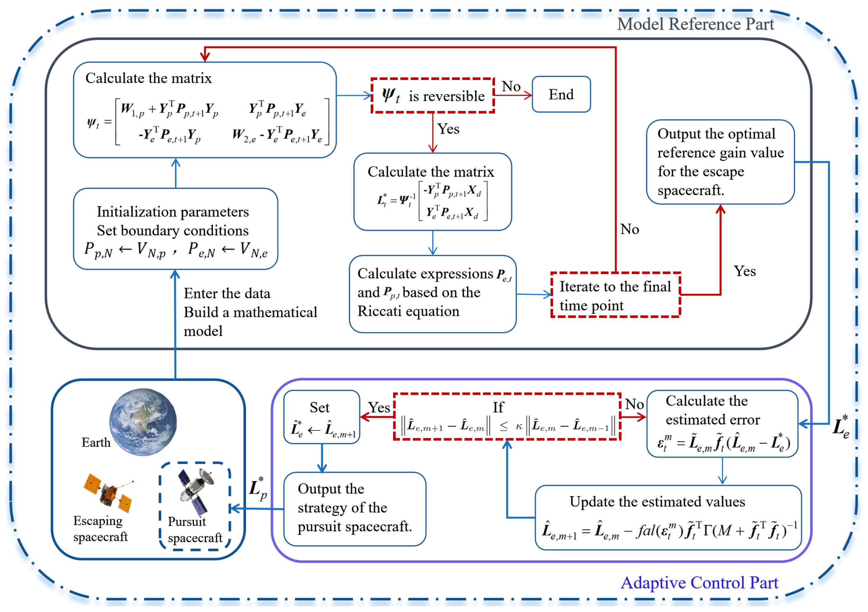
• Lines 3–9 (Offline Reference Calculation): The algorithm first calculates the optimal control gains for a finite horizon N. It iterates backward in time, computing the coupling matrix ${\mathit{\psi }}_t$ and solving for the optimal gains at each step using the Riccati updates from (7) and (8). This produces the optimal evader gain ${\mathit{L}}_e^{*}$, which will serve as the reference.
• Lines 10–18 (Online Pursuer Adaptation): This loop represents the online adaptive process. The pursuer evaluates the estimation error (line 11) and refines its estimate of the evader’s gain, ${\widehat{\mathit{L}}}_{e,m}$, using the robust update law from (37) (line 12).
• Lines 13–16 (Convergence Check): The adaptation continues until the change in the estimated gain becomes small, determined by the threshold $\kappa$. At this point, the algorithm has converged to a good estimate of the evader’s current strategy.
• Line 19 (Final Pursuer Strategy): With the best available estimate of the evader’s strategy, the pursuer calculates its own optimal control gain ${\mathit{L}}_p^{*}$ using Equation (13). This gain is then used to control the pursuer spacecraft.

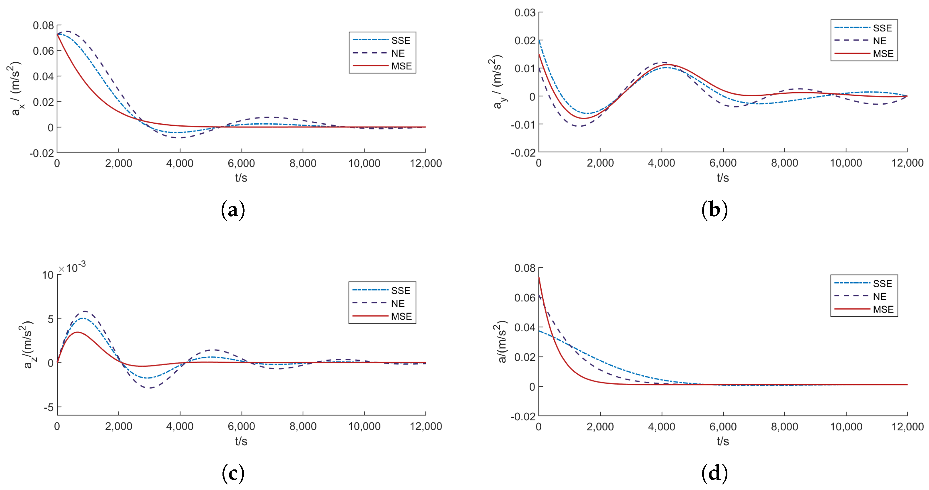
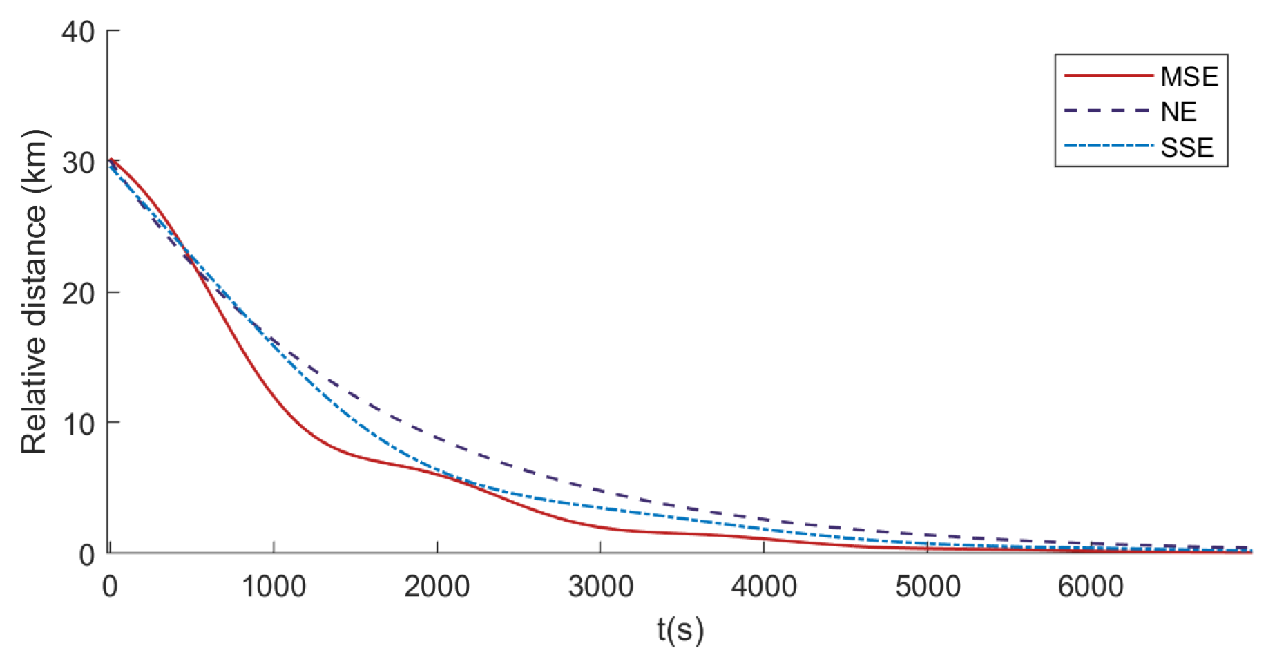
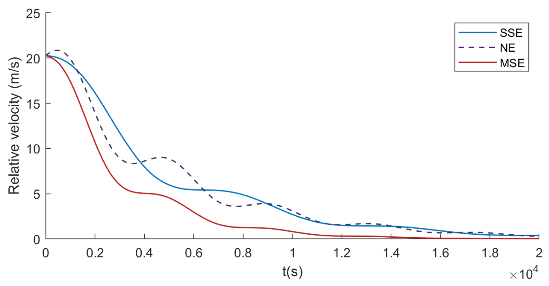
4. Simulation Experiment

The reference orbital radius in the spacecraft model is $a_0=8\times {10}^6\mathrm{km}$, the orbital angular velocity $\omega =7.2722\times {10}^{-5}\mathrm{rad}/\mathrm{s}$, the Earth’s gravitational constant $\mu =3.986\times {10}^{14}{\mathrm{m}}^2/{\mathrm{s}}^2$, and the sampling period $T=0.1\mathrm{s}$. The algorithm is set with the parameter ${\mathit{V}}_p={\mathit{V}}_{N,p}=\mathit{I}$, ${\mathit{W}}_{1,p}=\mathit{I}$, ${\mathit{W}}_{1,e}=100\mathit{I}$, ${\mathit{W}}_{2,p}=\mathit{I}$, ${\mathit{W}}_{2,e}=10\mathit{I}$ where $\mathit{I}$ denotes the unit matrix with appropriate dimensions. The initial state of the model is

$${\tilde{\mathit{f}}}_0=1000{\left[\begin{array}{cccccc}-76& -107& 48& 8& -6.1& -2.5\end{array}\right]}^{\mathrm{T}}$$

Number of iterations N = 100. According to the algorithm, the control gain can be obtained as follows:

$${\widehat{\mathit{L}}}_{e,100}=\left[\begin{array}{cccccc}7.66& -0.09& -0.13& 0.10& 0.31& -0.02\\ 15.6& -0.16& -0.11& 0.13& 0.67& -0.10\\ 0.00& 0.00& -0.28& 0.00& 0.00& 0.07\end{array}\right]$$

The Persistent Excitation condition is naturally satisfied in our simulation due to the evader’s dynamic maneuvers and the pursuer’s continuous adaptation, ensuring sufficient signal richness for parameter convergence. The initial relative states of the PE spacecraft are set as shown in

Table 2. Initial relative state of the pursuit and evader spacecraft.

Relative State	Pursuit	Evader
x (km)	10	0
y (km)	0	0
z (km)	0	0
$\dot{x}$ (m/s)	1.7	0
$\dot{y}$ (m/s)	4.3	0
$\dot{z}$ (m/s)	0	0

.

All simulation results presented are based on the initial conditions specified in Table 2 unless otherwise noted. For the performance comparison plots (Figure 4, Figure 5, Figure 6, Figure 7, Figure 8 and Figure 9), a single representative simulation run is shown to illustrate the typical dynamic behavior of the strategies.

Figure 4 demonstrates the simulation results of the model with reference to the MSE strategy algorithm. The figure describes the change rule of the relative motion state of the pursuer, and the results show that with the increase in the iteration number, the relative position finally tends to 0. This indicates that, under the designed game control strategy, by dynamically adjusting the control strategy, the pursuer, as a follower, is able to adapt to the actions of the evader, and gradually reduces the distance between the two. The pursuer finally achieves the pursuit of the evader.

In order to further verify the effectiveness of the proposed control algorithm, the model constructed in this paper is compared with the Stackelberg equilibrium–based (MSE) model reference adaptive control (MSE) algorithm and the single–step predictive Stackelberg equilibrium (SSE) algorithm [24] as well as the non–zero–sum Nash equilibrium (NE) algorithm [18], and the simulation results are now presented as follows.

Figure 5 illustrates the acceleration variations of the spacecraft in the three directions for the three strategies. The MSE algorithm takes into account the dynamic interaction between the pursuer and the evader, allowing the pursuer to respond quickly and take more aggressive actions in the early stages of the game, resulting in a large acceleration in the initial phase, followed by a rapid decrease and stabilization, which suggests that the strategy quickly adjusts the spacecraft state to match the motion of the evader in the initial phase.

Figure 6a illustrates the changes in the cost function of spacecraft pursuit over time for the three strategies. The MSE strategy has the fastest growing cost function, rising 53.71% faster than the SSE strategy in the 2000 s at the beginning of the game, and eventually stabilizing, suggesting that this strategy is advantageous in terms of cost–effectiveness, and it can also be seen that this strategy permits the evader to take a leadership position in the game, and by making positive adjustments in the early stages, it can reduce the distance to the evader more quickly, thereby reducing long–term costs. Figure 6b shows the fuel consumption of the pursuer for the three strategies. During the initial phase of the MSE strategy, fuel consumption increases rapidly, consistent with the strategy taking more aggressive action in the initial phase to respond quickly to the motion of the evader. Over time, the increase in fuel consumption slows down and stabilizes at a relatively low level. This demonstrates the advantage of the algorithm in the presence of fuel consumption constraints in spacecraft operations.

Figure 7 illustrates the relative distance between the two spacecraft over time. The relative distance decreases rapidly and tends to zero under the MSE strategy, and its speed of reducing the distance between the pursuing two spacecraft in 1200 s is 25.46% faster than the SSE strategy, and about 32.14% faster than the NE strategy, which shows its advantage in the efficiency of the pursuit. The rapid decrease in relative velocity helps the pursuer to match the evader’s velocity more quickly, leading to an effective pursuit.

Figure 8 shows the relative velocity changes between the two spacecraft. Consistent with the pursuit efficiency shown in Figure 7, the MSE strategy achieves the fastest reduction in relative velocity, decreasing 10.47% faster than the SSE strategy in the initial 3000 s. This rapid decrease is crucial for a successful capture, as it allows the pursuer to quickly match the evader’s velocity vector and stabilize the relative dynamics.

Figure 9 compares the computational time distributions of SSE, NE, MSE, and MPC, based on 100 Monte Carlo trials for each scenario. The boxplot shows that the median time (24.79 ms) of MSE is 7.36% and 39.11% lower than that of SSE (26.75 ms) and NE (40.7 ms), respectively, and the variance is smaller (MSE standard deviation 0.452 vs. 0.804 for NE), indicating its computational efficiency and stability advantages.

In order to further verify the anti–interference performance of the studied algorithm, the following data are set in the input signal of the algorithm to simulate the interference signals in the spacecraft PE game. The simulation parameters of the interference signals are shown in

Table 3. Interference factor settings.

Interference Factors	Description
Position measurement noise	$X\sim \mathcal{N}(50,100)$
The probability of signal loss	$5\%$
Signal delay time	$Y\sim \mathrm{Uniform}(20,40)$

. The position measurement noise is the interference inserted by the pursuit spacecraft when acquiring the position of the evader; the signal loss interference is the 5% probability that the pursuit spacecraft loses the signal from the evader at each iteration of the algorithm, and the signal delay interference denotes the time delay that occurs in receiving the motion state of the evader by the pursuit spacecraft.

Figure 10a compares the success rates of the three algorithms under different interference conditions. In the ‘No Interference’ case, the MSE algorithm achieves a lower success rate than the SSE algorithm. This result stems from the adaptive control mechanism of MSE, which continuously updates its parameters, while SSE relies on predictive optimization. MSE demonstrates stronger robustness, maintaining high performance under noise interference and signal loss, whereas NE and SSE exhibit significant performance degradation. Figure 10b analyzes the position error with standard deviation. MSE consistently satisfies the 20% safety threshold across all interference scenarios, including noise and signal loss. In contrast, NE and SSE show higher error variability, particularly under time delays. These results confirm the reliability of MSE in disturbance–prone environments.

5. Conclusions

This study presents a novel framework that synergizes Stackelberg game theory with the Riccati method and model reference adaptive control to resolve dynamic optimization challenges in spacecraft Pursuit–Evasion. By unifying these methodologies, the proposed MSE approach effectively addresses the intricacies of non–zero–sum games and $J_2$ perturbations, ensuring optimal control strategies under realistic conditions. This integration offers a significant advancement over conventional techniques by explicitly accounting for the sequential decision making and dynamic interplay between the spacecraft. Central to this work is a model–referenced adaptive control mechanism, enabling the pursuer to dynamically refine its strategy in real time based on the evader’s behavior. The optimal solution for the Stackelberg equilibrium is analytically derived through coupled Riccati equations, with rigorous proofs establishing its existence and uniqueness.

Extensive simulations validate the efficacy of the proposed method, demonstrating superior computational efficiency, minimal fuel expenditure, high pursuit success rates, and exceptional robustness against perturbations compared to NE and SSE strategies. These results underscore the method’s capability to deliver reliable and adaptive solutions for complex PE scenarios.

Despite the promising results, this work has limitations that open avenues for future research. The robustness analysis was conducted via scenario–based simulations; a direction for future work would be to formally integrate uncertainties like time delays into the system model itself and design a controller with certified robust stability guarantees. Additionally, the performance comparison could be expanded to include other optimal control benchmarks like Model Predictive Control (MPC). Future work will focus on addressing these areas to further enhance the practical applicability of the proposed framework.

References

1. Wong, K.K.L.; Chipusu, K. In-space cybernetical intelligence perspective on informatics, manufacturing and integrated control for the space exploration industry. J. Ind. Inf. Integr. 2024, 42, 100724. [Google Scholar] [CrossRef]
2. Ye, M.; Chen, C.L.P.; Zhang, T. Hierarchical Dynamic Graph Convolutional Network with Interpretability for EEG-Based Emotion Recognition. IEEE Trans. Neural Netw. Learn. Syst. 2022, 42, 1–12. [Google Scholar] [CrossRef]
3. Li, Q.; Yan, J.; Zhu, J.; Huang, T.; Zang, J. State of the Art and Development Trends of Top-Level Demonstration Technology for Aviation Weapon Equipment. Acta Aeronaut. Astronaut. Sin. 2016, 37, 1–15. [Google Scholar] [CrossRef]
4. Zhao, L.-R.; Dang, Z.-H.; Zhang, Y.-L. Orbital Game: Concepts, Principles and Methods. J. Command. Control 2021, 7, 215. [Google Scholar]
5. Vela, C.; Opromolla, R.; Fasano, G. A low-thrust finite state machine based controller for N-satellites formations in distributed synthetic aperture radar applications. Acta Astronaut. 2023, 202, 686–704. [Google Scholar] [CrossRef]
6. Yao, J.; Xu, B.; Li, X.; Yang, S. A clustering scheduling strategy for space debris tracking. Aerosp. Sci. Technol. 2025, 157, 109805. [Google Scholar] [CrossRef]
7. Zhou, X.; Yang, X.; Ye, X.; Li, B. Dual generative adversarial networks for merging ocean transparency from satellite observations. GISci. Remote Sens. 2024, 61, 1. [Google Scholar] [CrossRef]
8. Gu, Y.; Sun, X.; Fan, W. A fast star-ground coverage analysis method based on elevation angle visual element model. CEAS Aeronaut. J. 2025, 46, 330372. [Google Scholar] [CrossRef]
9. Kreps, D. Game theory and economic modelling. J. Econ. Educ. 1990, 23, 2. [Google Scholar] [CrossRef]
10. Başar, T.; Olsder, G.J. Dynamic Noncooperative Game Theory, 2nd ed.; 7. Stackelberg Equilibria of Infinite Dynamic Games; Society for Industrial and Applied Mathematics: Philadelphia, PA, USA, 1998; Volume 23, pp. 365–422. [Google Scholar] [CrossRef]
11. Abu-Khalaf, M.; Lewis, F.L.; Huang, J. Policy Iterations on the Hamilton–Jacobi–Isaacs Equation for State Feedback Control with Input Saturation. IEEE Trans. Autom. Control 2006, 51, 1989–1995. [Google Scholar] [CrossRef]
12. Li, H.; Liu, D.; Wang, D. Integral Reinforcement Learning for Linear Continuous-Time Zero-Sum Games with Completely Unknown Dynamics. IEEE Trans. Autom. Sci. Eng. 2014, 11, 706–714. [Google Scholar] [CrossRef]
13. Wei, Q.; Liu, D.; Lin, Q.; Song, R. Adaptive Dynamic Programming for Discrete-Time Zero-Sum Games. IEEE Trans. Neural Netw. Learn. Syst. 2018, 29, 957–969. [Google Scholar] [CrossRef] [PubMed]
14. Zhong, X.; He, H.; Wang, D.; Ni, Z. Model-Free Adaptive Control for Unknown Nonlinear Zero-Sum Differential Game. IEEE Trans. Cybern. 2018, 48, 1633–1646. [Google Scholar] [CrossRef] [PubMed]
15. Sun, Z.; Yang, S.; Piao, H.; Bai, C.; Ge, J. A survey of air combat artificial intelligence. Acta Aeronaut. Astronaut. Sin. 2021, 42, 25799. [Google Scholar] [CrossRef]
16. Xiong, T.; Zhang, R.; Liu, J.; Huang, T.; Liu, Y.; Yu, F.R. A blockchain-based and privacy-preserved authentication scheme for inter-constellation collaboration in Space-Ground Integrated Networks. Comput. Netw. 2022, 206, 108793. [Google Scholar] [CrossRef]
17. Hellmann, J.K.; Stiver, K.A.; Marsh-Rollo, S.; Alonzo, S.H. Defense against outside competition is linked to cooperation in male–male partnerships. Behav. Ecol. 2019, 31, 432–439. [Google Scholar] [CrossRef]
18. Zheng, Z.; Zhang, P.; Yuan, J. Nonzero-Sum Pursuit-Evasion Game Control for Spacecraft Systems: A Q-Learning Method. IEEE Trans. Aerosp. Electron. Syst. 2023, 59, 3971–3981. [Google Scholar] [CrossRef]
19. Wang, H.; Zhang, Y.; Liu, H.; Zhang, K. Impulsive thrust strategy for orbital pursuit-evasion games based on impulse-like constraint. Chin. J. Aeronaut. 2025, 38, 103180. [Google Scholar] [CrossRef]
20. Zhang, P.; Zhang, Y. Two-Step Stackelberg Approach for the Two Weak Pursuers and One Strong Evader Closed-Loop Game. IEEE Trans. Autom. Control 2024, 69, 1309–1315. [Google Scholar] [CrossRef]
21. Eltoukhy, A.E.; Wang, Z.; Chan, F.T.; Fu, X. Data analytics in managing aircraft routing and maintenance staffing with price competition by a Stackelberg-Nash game model. Transp. Res. Part E Logist. Transp. Rev. 2019, 122, 143–168. [Google Scholar] [CrossRef]
22. Han, C.; Huo, L.; Tong, X.; Wang, H.; Liu, X. Spatial Anti-Jamming Scheme for Internet of Satellites Based on the Deep Reinforcement Learning and Stackelberg Game. IEEE Trans. Veh. Technol. 2020, 69, 5331–5342. [Google Scholar] [CrossRef]
23. Hu, X.; Liu, S.; Xu, J.; Xiao, B.; Guo, C. Integral reinforcement learning based dynamic stackelberg pursuit-evasion game for unmanned surface vehicles. Alexandria Eng. J. 2024, 108, 428–435. [Google Scholar] [CrossRef]
24. Liu, Y.; Li, C.; Jiang, J.; Zhang, Y. A model predictive Stackelberg solution to orbital pursuit-evasion game. Chin. J. Aeronaut. 2025, 38, 103198. [Google Scholar] [CrossRef]
25. Lancaster, P.; Rodman, L. Algebraic Riccati Equations. Birkhäuser 2005, 108, 289–318. [Google Scholar] [CrossRef]
Figure 1. Schematic diagram of the pursuit and evasion process in the LVLH coordinate system.
Aerospace 12 00613 g001
Figure 2. Stackelberg equilibrium–based model reference adaptive control for spacecraft Pursuit–Evasion game flowchart.
Aerospace 12 00613 g002
Figure 3. Stackelberg equilibrium–based model reference adaptive control for spacecraft Pursuit–Evasion game timeline flowchart.
Aerospace 12 00613 g003
Figure 4. The law of the relative motion state of the Pursuit–Evasion spacecraft. (a) The law of variation of relative position with time steps. (b) Trajectory diagram of pursuit and evader.
Aerospace 12 00613 g004
Figure 5. Acceleration changes of spacecraft under three strategies. (a) The law of variation of a x . (b) The law of variation of a y . (c) The law of variation of a z . (d) The law of variation in the magnitude of acceleration.
Aerospace 12 00613 g005
Figure 6. Cost function and fuel consumption of pursuit spacecraft over time. (a) Pursuit spacecraft cost function over time. (b) Pursuit spacecraft fuel consumption curve over time.
Aerospace 12 00613 g006
Figure 7. The relative distance between the two spacecraft varies with time.
Aerospace 12 00613 g007
Figure 8. Relative velocity variation.
Aerospace 12 00613 g008
Figure 9. Time consumption in generating three strategies.
Aerospace 12 00613 g009
Figure 10. Comparative success rates of MSE, SSE, and NE algorithms under noise, signal loss, and time delay conditions.
Aerospace 12 00613 g010