Output Feedback Fuzzy Gain Scheduling for MIMO Systems Applied to Flexible Aircraft Control

Abstract

Previous works by our group evidenced stability problems associated with flight control law design for flexible aircraft regarding gain scheduling. This paper proposes an output feedback fuzzy-based gain scheduling approach to adequate closed-loop response in a broader range of the flight envelope. This method applies a variation of the controller gains based on the membership function design for all the varying parameters, such as dynamic pressure. It aims for performance improvement while enforcing global stability gain scheduling. The technique was demonstrated for the flexible ITA X-HALE aircraft nonlinear model and compared to the classical interpolation-based gain scheduling technique. The results revealed that fuzzy-based gain scheduling can effectively handle high-order systems while ensuring global system stability, leading to an overall improvement in performance.

1. Introduction

The flight dynamics of flexible aircraft are an area that has emerged in recent years to fill the gap left by the absence of an integrated treatment of classical flight dynamics [1]. With the industry demands to reduce fuel consumption and a growing interest in the aircraft class HALE (high-altitude, long-endurance), aircraft designs have become more lightweight with wings of an increasing aspect ratio that increase their flexibility [2].

Most aerospace vehicles developed since 1970 have some active closed-loop control system [1]. Furthermore, the control systems development for highly flexible aircraft requires more complex models and control techniques than those adopted for slightly flexible aircraft. Classically, control law design assumes a rigid airframe, accounting for steady aeroelastic effects, while dynamic aeroelastic interaction effects are only considered a posteriori, typically through gain stabilization, using low-pass and notch filters [3]. However, this procedure can lead to a low-performance controller when the flight and aeroelastic dynamics frequency ranges get closer to each other [3,4]. Several authors have addressed control law design based on flexible aircraft dynamics in the literature [3,4,5,6,7]. These approaches typically use structural state information as feedback signals in the control law. To maintain simplicity, some of them still apply linear control theory.

A problem in controller synthesis using linear techniques is that the linearized model represents the dynamics only in a region close to the operation point, in some cases leading to system instability when the model is subjected to significant variations, a common situation for flexible aircraft. A wide range of linear control techniques can address this issue, such as robust control, which deals with systems uncertainty [8,9,10]. Nonlinear techniques, such as adaptive control, can also be applied, which proposes predefined dynamics for the feedback gains that ensure stability and performance. These techniques often result in complex control laws that are hard to implement in practice [11,12].

Gain scheduling is the predominant method used in industry to develop a full-envelope flight control law [13]. For fixed-structure, linear-model-based controllers, gain scheduling is a good strategy since it continuously varies the controller coefficients, calculated for various operation points in the envelope, according to the current flight condition [14]. However, classical gain scheduling can cause abrupt changes in gains, which directly affect the dynamics of the model and may generate undesirable performance [15]. On the other side, previous fuzzy logic applications to gain scheduling in flight control demonstrated the feasibility of this approach [15,16,17,18]. The fuzzy membership functions provide the control parameters interpolation in a fuzzy-logic-based method that allows an adjustment for smoother controller-gains variation. Another advantage over classical gain scheduling is that closed-loop stability can be analytically guaranteed [19].

In this context, this paper proposes to investigate gain scheduling effectiveness via interpolation between design points, taking advantage of the fuzzy gain scheduling characteristic that allows a global stability analysis. Based on this characteristic, a method that combines performance and stability is proposed and evaluated. A similar method was first proposed for state feedback [20], and in this paper, it is extended to output feedback.

To carry out this investigation, the X-HALE (Experimental High-Altitude Long-Endurance) aircraft was used. This aircraft was conceived to be the University of Michigan (U-M) testbed to provide in-flight data to validate formulations for very flexible aircraft flight dynamics [2]. Flight tests of X-HALE have been carried out at U-M since the early 2010s. Jones and Cesnik [21] presented preliminary data obtained from the initial flight tests of a lightly instrumented X-HALE version. Furthermore, they conducted a comparative analysis between the flight test data and numerical results obtained using the U-M Nonlinear Aeroelastic Simulation Toolbox (UM/NAST). Unfortunately, due to the limited instrumentation available on the vehicle at that time, it was not possible to establish definitive correlations between theory and experimentation.

In 2014, the University of Michigan (U-M) and the Aeronautics Institute of Technology (ITA) in São José dos Campos, Brazil, formed an agreement, allowing ITA to build and test the X-HALE aircraft. While both U-M and ITA X-HALEs share a common airframe design, encompassing wing, boom, and tail, along with similar materials, airfoils, and dimensions, they exhibit notable distinctions in their electric, electronic, flight control, instrumentation, and propulsion systems. Flight tests of the four-meter-span ITA X-HALE-4 commenced in July 2017, offering insights into the complexities of flexible aircraft flight testing. Notably, this configuration intentionally lacks a rudder and has degraded lateral-directional handling qualities. In October 2019, flight tests of the six-meter-span ITA X-HALE-6 began, equipped with additional sensors, including strain gauges at four wing stations for bending and torsion strain measurement, and two extra all-moving horizontal tails, shown in Figure 1. As of the time of writing this paper, the ITA X-HALE-4 has flown 48 times, while the ITA X-HALE-6 has flown 4 times [22].

The proposed method is demonstrated for the flexible aircraft ITA X-HALE six-meter-span nonlinear model to schedule its stability augmentation system (SAS) gains and compared to the linear-interpolation-scheduling approach. The model used disregards the white vertical fins of the tail, which appear in the version shown in Figure 1. The results revealed that the approximation introduced in Section 2.4 enables the resolution of the LMI for higher-order systems (with 36 states) and that the methodology can guarantee and enhance the stability margins of the controller, as shown in Section 4.1.

This paper is organized as follows: Section 2 describes the theoretical development of the proposed controller design method, which includes an explanation of the fuzzy-logic-based gain scheduling, a proof of global stability, and the methodology for combining performance and stability. In Section 3, the numerical model and the performed order model reduction are briefly described. Section 4 presents the application of the methodology to the ITA X-XALE model, along with simulation results. Finally, the most important conclusions are presented in Section 5.

2. Theoretical Development

2.1. Linear Control Law Design

Flexible aircraft may exhibit undesirable flight dynamics characteristics stemming from various factors. In such instances, a viable recourse entails the implementation of an SAS aimed at enhancing stability margins and adjusting the aircraft’s behavior according to desired patterns.

To enhance stability and obtain an adequately damped response, a proportional output-feedback controller (block $\mathit{K}$ in Figure 2) is usually used in the inner-loop. A way to design the SAS gains is using the linear quadratic regulator (LQR) technique. First, the model is linearized, achieving the state-space system:

$$\begin{array}{cc}\hfill \dot{\mathit{x}}& =\mathit{Ax}+\mathit{Bu}\hfill \\ \hfill \mathit{y}& =\mathit{Cx}\hfill \end{array}$$

(1)

where A, B, and C are the state-space representation matrices, $\mathit{x}\in {\mathbb{R}}^n$ is the state vector, $\mathit{u}\in {\mathbb{R}}^m$ is the control input, and $\mathit{y}\in {\mathbb{R}}^p$ is the measured output [23]. The SAS control signal is the output feedback given the following:

$${\mathit{u}}_{\mathit{SAS}}=\mathit{Ky}$$

(2)

which leads to a closed loop given the following:

$$\dot{\mathit{x}}=(\mathit{A}+\mathit{BKC})\mathit{x}={\mathit{A}}_{\mathit{c}}\mathit{x}.$$

(3)

The LQR formulation allows the calculation of the feedback gain matrix $\mathit{K}$ by minimizing the performance index (PI) J, a cost function defined as follows:

$$J={\displaystyle \frac{1}{2}}{\int }_0^{\infty }({\mathit{x}}^{\mathit{T}}\mathit{Qx}+{\mathit{u}}^{\mathit{T}}\mathit{Ru})dt$$

(4)

where $\mathit{R}$ is a positive definite control weighting matrix, and $\mathit{Q}$ is a positive semidefinite state weighting matrix. The PI in the LQR problem can be calculated with the matrix $\mathit{P}$ obtained from the solution of the Lyapunov equation:

$$0={\mathit{A}}_{\mathit{c}}^{\mathit{T}}\mathit{P}+{\mathit{PA}}_{\mathit{c}}+\mathit{Q}-{\mathit{C}}^{\mathit{T}}{\mathit{K}}^{\mathit{T}}\mathit{RKC}$$

(5)

A gain matrix that minimizes the PI is desired. If the closed-loop system is asymptotically stable, the PI can be calculated with the following equation:

$$J={\displaystyle \frac{1}{2}}{\mathit{x}}^{\mathit{T}}\left(0\right)\mathit{Px}\left(0\right)={\displaystyle \frac{1}{2}}tr\left(\mathit{Px}\left(0\right){\mathit{x}}^{\mathit{T}}\left(0\right)\right)$$

(6)

If the model is open-loop unstable, an initial stabilizing gain is calculated by minimizing the maximum real part of the eigenvalues of ${\mathit{A}}_{\mathit{c}}$. Then, Equation (5) is solved numerically in an iterative process to minimize J in Equation (6) [23].

2.2. The Gain Scheduling Problem

Linearized models cannot represent the entire flight envelope due to significant changes in the dynamic pressure during operation, which considerably modify the rigid body and aeroelastic dynamics. As a result, a constant linear model cannot be used to describe the entire flight envelope, and traditional methods with a fixed gain set cannot fulfill the design requirements [14]. Gain scheduling, whose principle is adjusting the control law with the change in the scheduling variable, is a control technique that enables the control parameters interpolation between different design points to accomplish satisfactory control tasks.

2.2.1. Classical Gain Scheduling

A gain-scheduled controller design for a nonlinear model can be described as a four-step procedure. The first step is to compute a linearization of the nonlinear model in the desired equilibrium points, also called operating points or set points. The second step uses linear design methods to design linear controllers for each linear model obtained in the previous step to achieve the requirements for each equilibrium condition. The third step consists of implementing the linear controller family such that the controller coefficients (gains) are varied (scheduled) according to the current value of the scheduled variables [14], represented in Figure 2 by “GS”. Finally, the fourth step is performance and stability evaluation. Typically, stability can be assured only locally and in a slow-variation setting, but it is by no means guaranteed. The same applies to control performance. Depending on the scheduling strategy, performance may fall drastically [15]. Normally, stability and performance must be assessed based on simulation studies [14]. Depending on the number of parameters that may vary and change the model, the number of simulations to be performed may increase drastically, resulting in a very costly control law development process.

2.2.2. Fuzzy-Logic-Based Gain Scheduling (FGS)

The fuzzy logic is based on “IF antecedent THEN consequence” rules, and any rule is composed of an antecedent and a consequence, where both can receive more than one preposition. Among the fuzzy logic classes, the Takagi–Sugeno (TS) one involves the particularity of containing a linear input-output relation in the consequence [24].

The FGS controller that we propose in this paper is a TS-type fuzzy controller, and it follows the same steps as the classical gain scheduling. However, it employs a different interpolation strategy, which enables a stability analysis of the fuzzy model [19].

At each design point, $y_{g{s}_i}(i=1,2,\dots ,l)$, with l design variable points, the system described in Equation (1) is approximated using the fuzzy rule as follows below:

$$R_i:\mathrm{If}y\mathrm{is}{y}_{g{s}_i}\mathrm{then}\dot{\mathit{x}}={\mathit{A}}_i\mathit{x}+{\mathit{B}}_i\mathit{u}\mathrm{and}\mathit{y}={\mathit{C}}_i\mathit{x}$$

(7)

where $R_i$ is the $i^{th}$ rule, $y_{g{s}_i}$ is the fuzzy set for each rule, “y is $y_{g{s}_i}$” is the antecedent (given that y is the scheduled variable crisp value) and “$\dot{\mathit{x}}={\mathit{A}}_i\mathit{x}+{\mathit{B}}_i\mathit{u}\mathrm{and}\mathit{y}={\mathit{C}}_i\mathit{x}$” is the consequence, with two linear input-output relations. The control law is defined as follows:

$$R_i:\mathrm{If}y\mathrm{is}{y}_{g{s}_i}\mathrm{then}\mathit{u}={\mathit{K}}_i\mathit{y}$$

(8)

The membership functions used to interpolate the rules can have many forms (triangular, trapezoidal, bell, Gaussian, etc). The Gaussian form was selected in this work because it ensures a smooth transition between gains while emphasizing the influence of the closest design point. The corresponding weights are given as follows:

$${\mu }_i\left(v\right)=exp\left(-{\left({\displaystyle \frac{y-y_{g{s}_i}}{2\sigma }}\right)}^2\right)$$

(9)

The weight is the mathematical form to ponder each rule according to the scheduled variable value, and $\sigma$ (standard deviation) is a design parameter that measures how the neighbor antecedents affect the consequence. If $\sigma$ is too small, the controller’s transition becomes excessively sharp. Conversely, if $\sigma$ is too large, the influence of nearby design points may exceed the desired level. We selected a set of $\sigma$ values such that, at the design point, the weight of the nearest neighbors approaches zero, while at the midpoint, both points are assigned equal weight. In Figure 3, seven membership functions ($\mu$), one for each velocity selected, with Gaussian form, are displayed, and the weight for each rule is given by $\mu$. Eventually, the weights are normalized by the sum of all rules’ weights so that the sum of all normalized weights is always equal to 1. Therefore, the normalized weights ${\omega }_i$ are given as follows:

$${\omega }_i={\displaystyle \frac{{\mu }_i}{{\sum }_{i=1}^l{\mu }_i}}$$

(10)

The system can now be represented as follows:

$$\dot{\mathit{x}}=\sum _{i=1}^l{\omega }_i({\mathit{A}}_i\mathit{x}+{\mathit{B}}_i\mathit{u}),$$

(11)

$$\mathit{y}=\sum _{i=1}^l{\omega }_i\left({\mathit{C}}_i\mathit{x}\right),$$

(12)

and the control law as follows:

$$\mathit{u}=\sum _{i=1}^l{\omega }_i\left({\mathit{K}}_i\mathit{y}\right).$$

(13)

The FGS controller effectiveness relies on tuning both the LQR controllers and $\sigma$. The LQR parameter affects the performance and stability at each design point (one LQR design for each fuzzy rule), and $\sigma$ tunes how smooth the transition between these points will be.

2.3. Fuzzy Gain Scheduling Design Taking into Account Global Stability

The closed-loop stability assessment is based on the Lyapunov direct method. The Lyapunov direct method seeks to determine the Lyapunov function parameters belonging to a particular candidate class that guarantees the stability of the investigated system [25]. This analysis will be conducted starting from a Lyapunov candidate in the quadratic form,

$$\begin{array}{c}\hfill V={\mathit{x}}^{\mathit{T}}\mathit{Px}\end{array}$$

(14)

and then proceeding according to the second Lyapunov method [26].

Therefore, the parameterization occurs in the search for a single symmetric positive definite matrix $\mathit{P}$, which simultaneously satisfies a constraint set in the form of linear matrix inequalities (LMI). For the open-loop system described in Equation (11), the time derivative of the Lyapunov candidate function will be

$$\begin{array}{cc}\hfill \dot{V}& ={\dot{\mathit{x}}}^T\mathit{Px}+{\mathit{x}}^T\mathit{P}\dot{\mathit{x}}\hfill \end{array}$$

(15)

$$\begin{array}{cc}\hfill & ={\mathit{x}}^T\mathit{A}{\left(\omega \right)}^T\mathit{Px}+{\mathit{x}}^T\mathit{PA}\left(\omega \right)\mathit{x}\hfill \end{array}$$

(16)

$$\begin{array}{cc}\hfill & ={\mathit{x}}^T[\mathit{A}{\left(\omega \right)}^T\mathit{P}+\mathit{PA}\left(\omega \right)]\mathit{x}\hfill \end{array}$$

(17)

$$\begin{array}{cc}\hfill & ={\mathit{x}}^T\sum _{i=1}^l{\omega }_i[{{\mathit{A}}_{\mathit{i}}}^T\mathit{P}+{\mathit{PA}}_{\mathit{i}}]\mathit{x}\hfill \end{array}$$

(18)

where $\mathit{A}\left(\omega \right)$ is the final value of all the fuzzy rules, $\mathit{A}\left(\omega \right)={\sum }_{i=1}^l{\omega }_i{\mathit{A}}_{\mathit{i}}$. This notation will also find application in subsequent matrices.

Since the ${\sum }_{i=1}^l{\omega }_i$ is always equal to one, see Equation (10), rather than satisfying Equation (18), it would suffice to satisfy the Theorem presented below, which involves a set of coupled Lyapunov inequalities to ensure stability in the Lyapunov sense.

Theorem 1

([25]). The system represented in Equation (11) is asymptotically stable if there is a symmetric positive definite matrix, $\mathit{P}$, that satisfies

$$\begin{array}{c}\hfill {{\mathit{A}}_{\mathit{i}}}^T\mathit{P}+{\mathit{PA}}_{\mathit{i}}<0,i=1,2,\dots ,l.\end{array}$$

(19)

In order to calculate the controller gains, first for state feedback, they will be inserted into the derivative of the Lyapunov function in Equation (16) for the closed-loop case, resulting in the following:

$$\begin{array}{cc}\hfill \dot{V}& ={\mathit{x}}^T{[\mathit{A}\left(\omega \right)+\mathit{B}\left(\omega \right)\mathit{K}\left(\omega \right)]}^T\mathit{Px}+{\mathit{x}}^T\mathit{P}[\mathit{A}\left(\omega \right)+\mathit{B}\left(\omega \right)\mathit{K}\left(\omega \right)]\mathit{x}\hfill \end{array}$$

(20)

$$\begin{array}{cc}\hfill & ={\mathit{x}}^T({[\mathit{A}\left(\omega \right)+\mathit{B}\left(\omega \right)\mathit{K}\left(\omega \right)]}^T\mathit{P}+\mathit{P}[\mathit{A}\left(\omega \right)+\mathit{B}\left(\omega \right)\mathit{K}\left(\omega \right)])\mathit{x}.\hfill \end{array}$$

(21)

Therefore, it is enough to ensure

$$\begin{array}{c}\hfill {[\mathit{A}\left(\omega \right)+\mathit{B}\left(\omega \right)\mathit{K}\left(\omega \right)]}^T\mathit{P}+\mathit{P}[\mathit{A}\left(\omega \right)+\mathit{B}\left(\omega \right)\mathit{K}\left(\omega \right)]<0.\end{array}$$

(22)

At this point, it is noted that the inequality is not an LMI since there are two matrix variable sets to be determined that are multiplied: one being the matrix $\mathit{K}\left(\omega \right)$ and the other being the matrix $\mathit{P}$. The simplicity through which such inequalities can be converted into LMI is the great attraction of quadratic stability. Using the transformations $\mathit{W}={\mathit{P}}^{-1}$ and $\mathit{Z}\left(\omega \right)=\mathit{K}\left(\omega \right)\mathit{W}$, the equivalent condition is obtained:

$$\begin{array}{c}\hfill \mathit{Z}{\left(\omega \right)}^T\mathit{B}{\left(\omega \right)}^T+\mathit{WA}{\left(\omega \right)}^T+\mathit{A}\left(\omega \right)\mathit{W}+\mathit{B}\left(\omega \right)\mathit{Z}\left(\omega \right)<0\end{array}$$

(23)

$$\begin{array}{c}\hfill \sum _{i=1}^l\sum _{j=1}^l{\omega }_i{\omega }_j({\mathit{Z}}_{\mathit{j}}^T{\mathit{B}}_{\mathit{i}}^T+{\mathit{WA}}_{\mathit{i}}^T+{\mathit{A}}_{\mathit{i}}\mathit{W}+{\mathit{B}}_{\mathit{i}}{\mathit{Z}}_{\mathit{j}})<0\end{array}$$

(24)

Thus, the following theorem was achieved, given that a linear set of inequalities in the $\mathit{W}$ and ${\mathit{Z}}_{\mathit{i}}$ variables is now available.

Theorem 2

([25]). The system represented in Equation (11) is asymptotically stable if there is a symmetric positive definite matrix $\mathit{W}$ and any matrices ${\mathit{Z}}_{\mathit{i}}$ that satisfy

$$\begin{array}{c}\hfill {\mathit{WA}}_{\mathit{i}}^T+{\mathit{A}}_{\mathit{i}}\mathit{W}+{\mathit{Z}}_{\mathit{i}}^T{\mathit{B}}_{\mathit{i}}^T+{\mathit{B}}_{\mathit{i}}{\mathit{Z}}_{\mathit{i}}<0,i=j=1,2,\dots ,l.\\ \hfill {\mathit{WA}}_{\mathit{i}}^T+{\mathit{A}}_{\mathit{i}}\mathit{W}+{\mathit{WA}}_{\mathit{j}}^T+{\mathit{A}}_{\mathit{j}}\mathit{W}+{\mathit{Z}}_{\mathit{j}}^T{\mathit{B}}_{\mathit{i}}^T+{\mathit{B}}_{\mathit{i}}{\mathit{Z}}_{\mathit{j}}+{\mathit{Z}}_{\mathit{i}}^T{\mathit{B}}_{\mathit{j}}^T+{\mathit{B}}_{\mathit{j}}{\mathit{Z}}_{\mathit{i}}<0,i<j,i=j=1,2,\dots ,l.\end{array}$$

(25)

Suppose that there is a feasible solution to the inequalities presented in Theorem 2. In that case, the stabilizing controller gains can be obtained by solving ${\mathit{K}}_{\mathit{i}}={\mathit{Z}}_{\mathit{i}}{\mathit{W}}^{-1}$ and also the Lyapunov function that guarantees stability to the closed-loop system for these projected gains, obtained from the inverse of $\mathit{W}$.

However, there are situations where the state feedback controller is restricted since it would be necessary to use state observers for a large number of states. That is the case of flexible aircraft dynamic models, which usually have a high-order model. Thus, we adapt the method for the output feedback case in the following section.

2.4. Fuzzy Gain Scheduling with Output Feedback

Considering the feedback of only the measured outputs, given via the output matrix $\mathit{C}$, the Lyapunov candidate in Equation (21) is expanded as follows:

$$\begin{array}{cc}\hfill & \hfill \mathit{W}{[\mathit{A}\left(\omega \right)+\mathit{B}\left(\omega \right)\mathit{K}\left(\omega \right)\mathit{C}\left(\omega \right)]}^T+[\mathit{A}\left(\omega \right)+\mathit{B}\left(\omega \right)\mathit{K}\left(\omega \right)\mathit{C}\left(\omega \right)]\mathit{W}<0.\end{array}$$

(26)

$$\begin{array}{c}\hfill \mathit{A}\left(\omega \right)\mathit{W}+\mathit{W}\mathit{A}{\left(\omega \right)}^T+\mathit{B}\left(\omega \right)\mathit{K}\left(\omega \right)\mathit{C}\left(\omega \right)\mathit{W}+\mathit{W}\mathit{C}{\left(\omega \right)}^T\mathit{K}{\left(\omega \right)}^T\mathit{B}{\left(\omega \right)}^T<0.\end{array}$$

(27)

The stability condition is no longer a set of LMI since both $\mathit{K}\left(\omega \right)$ and $\mathit{W}$ are variables. A similar problem was faced in the previous section. The solution is also similar, transforming the variables until a set of LMI was achieved. To transform these inequalities to LMI, two transformations are necessary [27], the first being $\mathit{MC}=\mathit{CW}$, where $\mathit{C}$ must be full row rank, resulting in the following:

$$\begin{array}{c}\hfill \mathit{A}\left(\omega \right)\mathit{W}+\mathit{W}\mathit{A}{\left(\omega \right)}^T+\mathit{B}\left(\omega \right)\mathit{K}\left(\omega \right)\mathit{M}\left(\omega \right)\mathit{C}\left(\omega \right)+\mathit{C}{\left(\omega \right)}^T\mathit{M}{\left(\omega \right)}^T\mathit{K}{\left(\omega \right)}^T\mathit{B}{\left(\omega \right)}^T<0,\end{array}$$

(28)

and the second $\mathit{K}=\mathit{N}{\mathit{M}}^{-1}$, resulting in the following LMI:

$$\begin{array}{c}\hfill \mathit{A}\left(\omega \right)\mathit{W}+\mathit{W}\mathit{A}{\left(\omega \right)}^T+\mathit{B}\left(\omega \right)\mathit{N}\left(\omega \right)\mathit{C}\left(\omega \right)+\mathit{C}{\left(\omega \right)}^T\mathit{N}{\left(\omega \right)}^T\mathit{B}{\left(\omega \right)}^T<0.\end{array}$$

(29)

However, these transformations include an equality relation, $\mathit{MC}=\mathit{CW}$. In order to keep the LMI set as simple as possible, once the system already has high order and complexity, that equality was converted into an approximate LMI.

$$\begin{array}{cc}\hfill & \hfill \mathit{M}\left(\omega \right)\mathit{C}\left(\omega \right)=\mathit{C}\left(\omega \right)\mathit{W},\end{array}$$

(30)

$$\begin{array}{c}\hfill \mathit{M}\left(\omega \right)\mathit{C}\left(\omega \right)-\mathit{C}\left(\omega \right)\mathit{W}=0.\end{array}$$

(31)

This equality can be approximated as follows:

$$\begin{array}{c}\hfill \left[\begin{array}{cc}-\kappa \mathit{I}& {[\mathit{M}\left(\omega \right)\mathit{C}\left(\omega \right)-\mathit{C}\left(\omega \right)\mathit{W}]}^T\\ \left[\mathit{M}\right(\omega \left)\mathit{C}\right(\omega )-\mathit{C}(\omega \left)\mathit{W}\right]& -\mathit{I}\end{array}\right]<0.\end{array}$$

(32)

The left-hand-side matrix in the LMI is a Hermitian or real symmetric matrix, and the inequality aims to ensure that it is negative definite, which makes this approximation valid. This occurs because, under these conditions, the matrix has two key properties [28]:

• All diagonal elements must be less than 0, which implies $\kappa >0$;
• The matrix must be diagonally dominant; in other words, the matrix largest magnitude value elements must be at the main diagonal.

The second property delineated above underscores the dependency of the approximation of Equation (31) on the variable $\kappa$. Consequently, the overarching objective is to achieve a small positive value for $\kappa$, ensuring the convergence of the right-hand side of Equation (31) towards zero. It is, nevertheless, imperative to strike a judicious balance to prevent $\kappa$ from diminishing to an extent that might render the LMI infeasible. With the approximation proposed, the following LMI sets were obtained:

$$\begin{array}{c}\hfill \begin{array}{c}\hfill {\mathit{A}}_i\mathit{W}+\mathit{W}{\mathit{A}}_i^T+{\mathit{B}}_i{\mathit{N}}_i\mathit{C}+{\mathit{C}}^T{\mathit{N}}_i^T{\mathit{B}}_i^T<0,i=j=1,2,\dots ,l;\\ \hfill {\mathit{WA}}_{\mathit{i}}^T+{\mathit{A}}_{\mathit{i}}\mathit{W}+{\mathit{WA}}_{\mathit{j}}^T+{\mathit{A}}_{\mathit{j}}\mathit{W}+{\mathit{C}}^T{\mathit{N}}_j^T{\mathit{B}}_i^T+{\mathit{B}}_i{\mathit{N}}_j\mathit{C}+\\ \hfill {\mathit{C}}^T{\mathit{N}}_i^T{\mathit{B}}_j^T+{\mathit{B}}_j{\mathit{N}}_i\mathit{C}<0,i<j,i=j=1,2,\dots ,l;\\ \hfill \left[\begin{array}{cc}-\kappa \mathit{I}& {[\mathit{M}\mathit{C}-\mathit{C}\mathit{W}]}^T\\ [\mathit{M}\mathit{C}-\mathit{C}\mathit{W}]& -\mathit{I}\end{array}\right]<0.\end{array}\end{array}$$

(33)

Solving the LMI set, the gains can be recovered using the relation ${\mathit{K}}_{\mathit{i}}={\mathit{N}}_{\mathit{i}}{\mathit{M}}^{-1}$, where ${\mathit{N}}_{\mathit{i}}$ and $\mathit{M}$ are accessed directly from the LMI resolution. Note also that a constant $\mathit{C}$ matrix is assumed for all design points in this formulation, which reduces the number of LMI to be solved. In cases where the output matrices vary across different design points, the formulation can still be applied. However, in such cases, an approximation, as represented in Equation (32), must be employed for each distinct output matrix, as there will be l equations of the form $M_i{C}_i=C_{i}W$.

Therefore, the LMI set, Equation (33), enables a design that guarantees the global asymptotic stability for a nonlinear system described according to Equations (11)–(13).

2.5. A New FGS Methodology Combining Stability and Performance

Despite the global stability, the method discussed so far does not introduce any performance requirement. The resulting gains may present an inadequate response. In this sense, studies [29,30] have been carried out to insert performance criteria in the solution of these equations, unfortunately resulting in a considerable increase in the computational cost of the method. We propose here an efficient way of including a performance specification in the solution.

Combining the set of LMI shown in Equation (33), and a focus on performance improvement through LQR, a methodology for designing a fuzzy gain scheduling controller is proposed following the steps shown in the flowchart in Figure 4:

• The initial step involves selecting a set of state-space representations of the system to ensure an effective representation of the original system;
• Subsequently, the second step entails the minimization of the PI for each design point;
• The concluding step involves the computation of stabilizing gains utilizing LMI (Equation (33)). In this phase, the system is considered in closed-loop configuration, incorporating gains determined in the preceding step. An additional gain is then calculated to ensure global asymptotic stability of the system.

The resulting gain matrix can be expressed as follows:

$$\begin{array}{c}\hfill \mathit{K}={\mathit{K}}_{\mathit{LQR}}+{\mathit{K}}_{\mathit{LMI}}\end{array}$$

(34)

Through this approach, the delta gains obtained from the LMI formulation represent adjustments to the nominal controller parameters. Small delta gains imply that the adapted controller closely approximates the behavior of the optimal controller derived from the LQR design, thereby minimizing performance degradation. However, it is important to emphasize that, while the LMI framework ensures the global stability of the closed-loop system, it does not inherently guarantee that the delta gains will be small. Consequently, a trade-off emerges: although global stability is achieved through the LMI solution, this may come at the cost of a deviation from the optimal LQR parameters.

3. ITA X-HALE Model

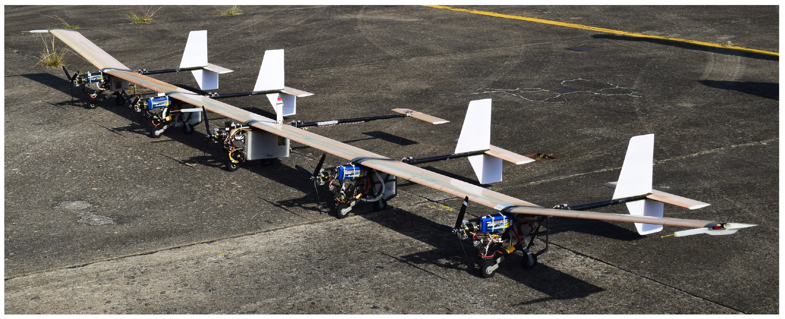
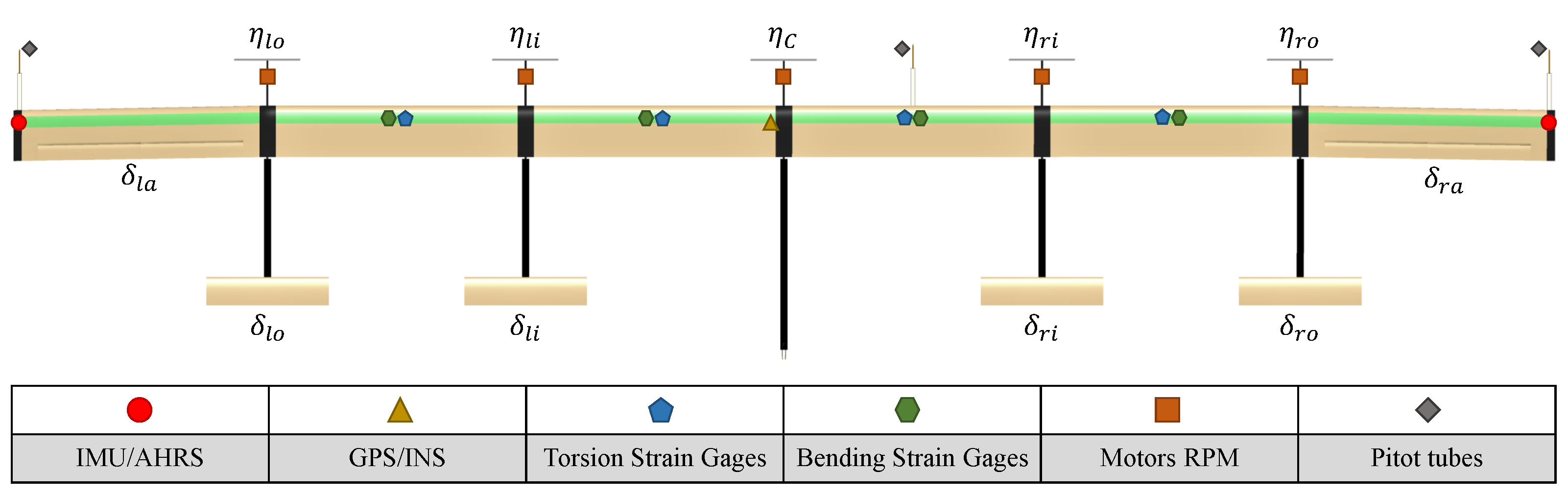
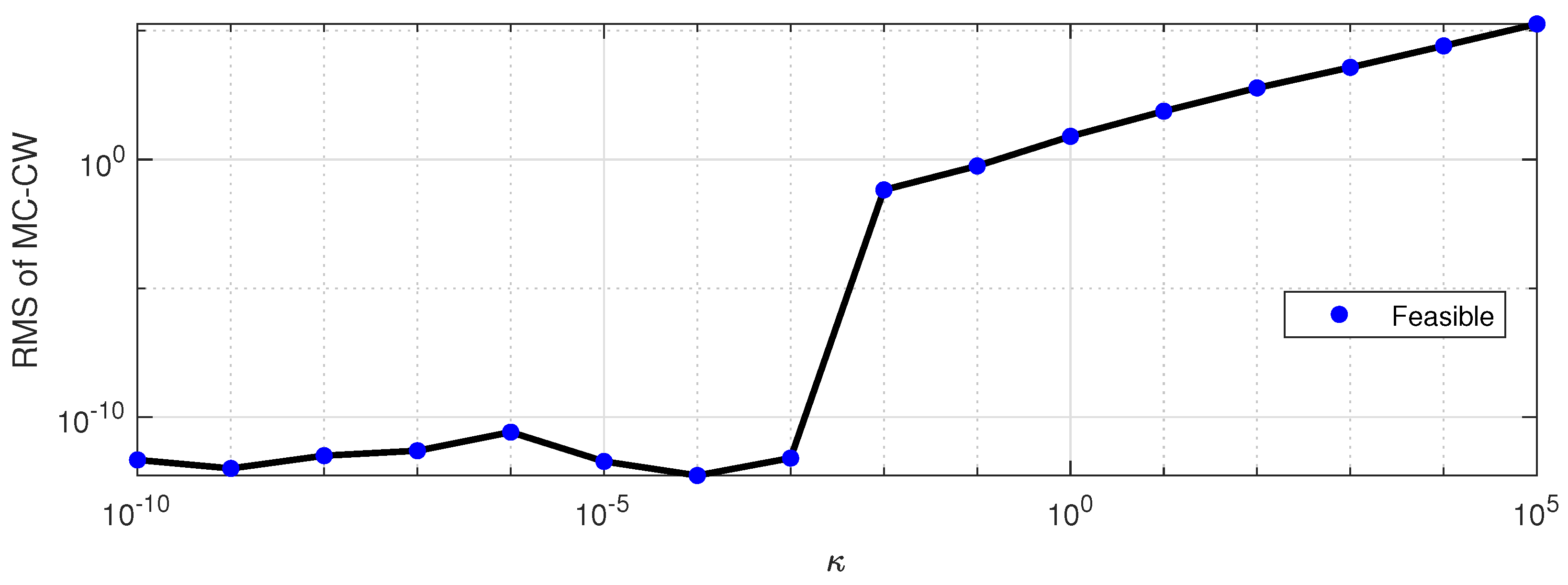
The ITA X-HALE aircraft, illustrated in Figure 1, has a total mass of 12.363 kg. Its modular wing design consists of six segments, each with a span of 1.0 m and a chord of 0.2 m. Electric motors, landing gear, and onboard electronics are housed in pods located at the junctions between adjacent modules. Attached to these pods are booms that extend rearward, each supporting a tail assembly at its tip. The central tail can be fixed either in a horizontal or vertical position to adjust the aircraft’s lateral–directional characteristics. In this study, the central tail is fixed in the vertical position. The side tails are all-moving control surfaces, known as elevons, capable of providing both longitudinal and lateral–directional control. The outermost wing modules incorporate a 10° dihedral angle, and the entire wing is mounted with a 5° incidence angle. The wing uses the EMX-07 reflexed airfoil, while the tail surfaces are based on the NACA 0012 airfoil.

In the X-HALE-6 configuration, the aircraft features six wing modules, five pods, and four side tails. To enhance operational safety and improve lateral–directional stability, dorsal, and ventral vertical fins were added at the ends of the four side booms, as shown in Figure 1.

3.1. Model Description

The mathematical formulation used to model the ITA X-HALE flight dynamics is based on the equations of motion derived for dually constrained axes [4,31]. In this formulation, the origin, S, of the structural axes, corresponding to a material point without elastic displacement, can be non-coincident with the origin O of the body axes used in the equations of motion. In calculating equilibrium conditions, all the structural degrees of freedom are considered. In modeling the nonlinear flight dynamics around equilibrium, a reduced set of inertia-relieved constrained modes of vibration [4,31] are retained.

The aerodynamic model of the aircraft is based both on the doublet-lattice method [32] and on the vortex-lattice method [33] to which the former reduces at zero frequency. Rational function approximations [31,34] make the representation of aerodynamic loads possible in the time domain. Consequently, a significant number of aerodynamic lag states arise to make the approximation sufficiently accurate. The induced drag is also modeled based on the method of Ref. [35].

The wing structural–dynamic model consists of beam finite elements along the span. Beam elements are also used for the connection between the wing and the booms and for the booms themselves. The horizontal tails are modeled with rigid elements. Small deformations are assumed.

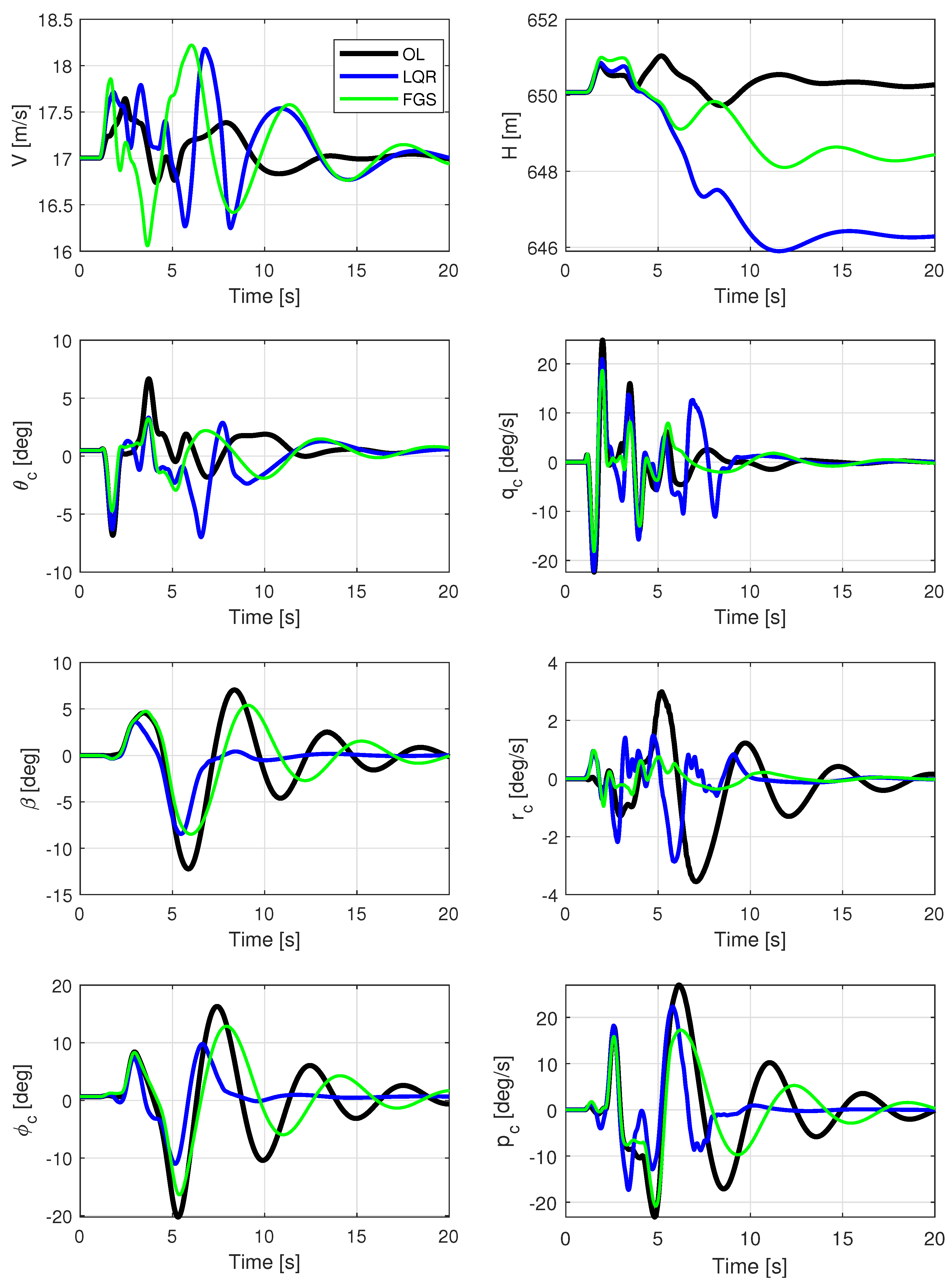
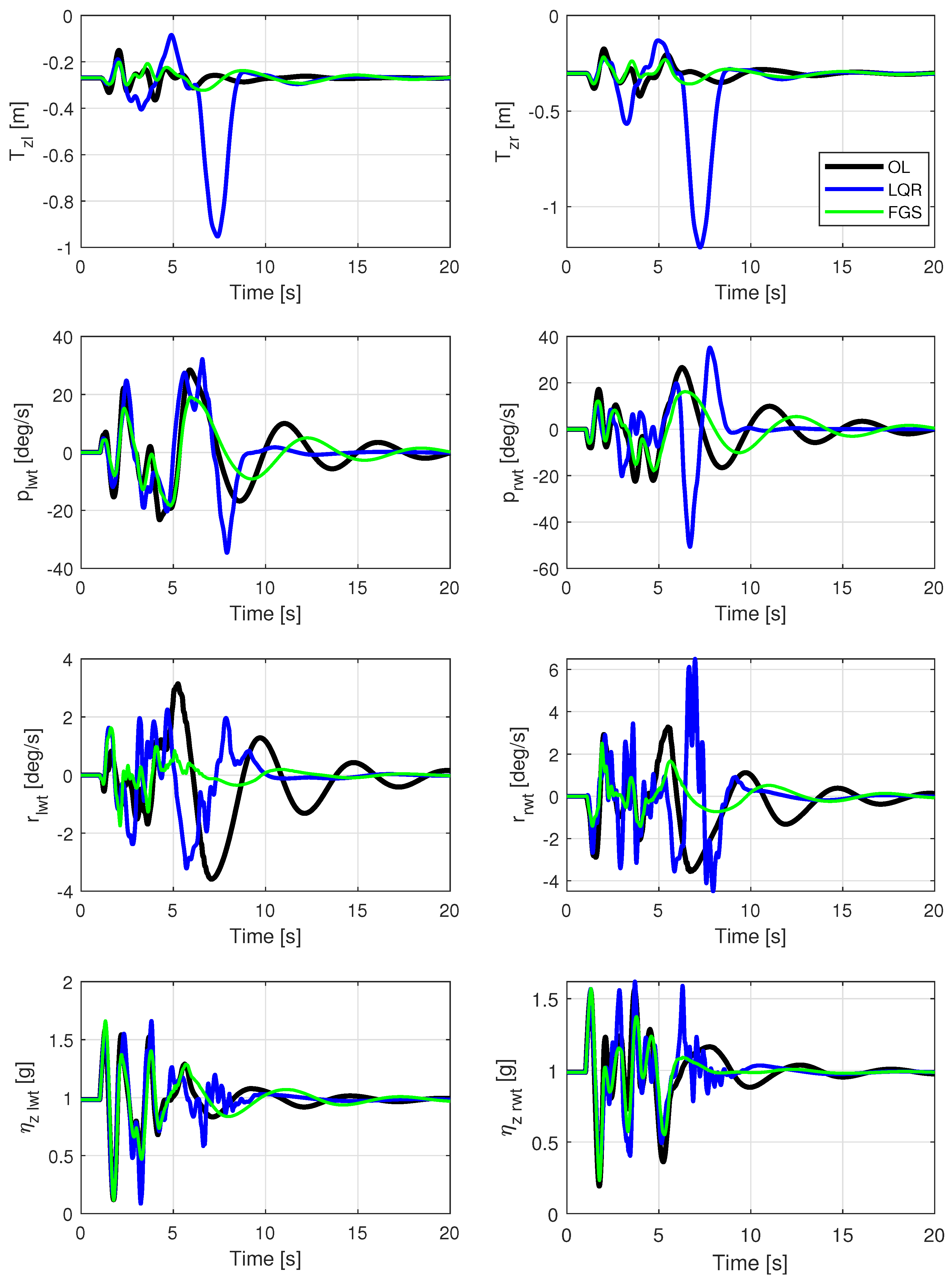
For control system design purposes, linear-time-invariant realizations of the nonlinear model under small disturbances around different equilibrium flight conditions are considered for the six-meter-span aircraft with a vertical central tail. The system of linear equations is then given as follows:

$$\begin{array}{ccc}\hfill \dot{\mathit{x}}& =& \mathit{Ax}+{\mathit{Bu}}_{\mathit{ctrl}}\hfill \end{array}$$

(35)

$$\begin{array}{ccc}\hfill \mathit{y}& =& \mathit{Cx}+{\mathit{Du}}_{\mathit{ctrl}}\hfill \end{array}$$

(36)

where $\mathit{A}\in {\mathbb{R}}^{n\times n}$ is the state matrix, $\mathit{B}\in {\mathbb{R}}^{n\times m}$ is the control matrix, $\mathit{C}\in {\mathbb{R}}^{p\times n}$ is the output matrix and $\mathit{D}\in {\mathbb{R}}^{p\times m}$ is the direct-feed matrix.

The vector of disturbances of the state variables around the equilibrium conditions is given as follows:

$$\mathit{x}={\left[V\alpha q\theta Hx\beta \varphi pr\psi y{{\mathit{\lambda }}_{\mathit{rb}}}^T{\mathit{\eta }}^T{\dot{\mathit{\eta }}}^T{{\mathit{\lambda }}_{\mathit{\eta }}}^T\right]}^T$$

(37)

where $\mathit{x}\in {\mathbb{R}}^{n\times 1}$ and disturbances with respect to the equilibrium states are implicit.

The model includes the kinematic equations in the inertial reference frame for all six rigid-body degrees of freedom: displacements in the x and y directions, altitude H, and roll, pitch, and yaw angles ($\varphi$, $\theta$, and $\psi$, respectively). Furthermore, the velocity, V, the angle of attack, $\alpha$, the sideslip angle, $\beta$, as well as the angular rates p, q, and r also have their corresponding equations of motion. The structural dynamics are represented by modal coordinates. The modal amplitudes and their time derivatives are given by $\mathit{\eta }$ and $\dot{\mathit{\eta }}$, respectively. Modes of vibration with frequencies up to 25 Hz is retained in the model. Aerodynamic lag states due to rigid-body and control-surface dynamics (${\mathit{\lambda }}_{\mathit{rb}}$) and due to the aeroelastic dynamics (${\mathit{\lambda }}_{\mathit{\eta }}$) are also included. Guimarães Neto et al. [22] make a more in-depth description of the model and also present a validation of the numerical results with flight test data.

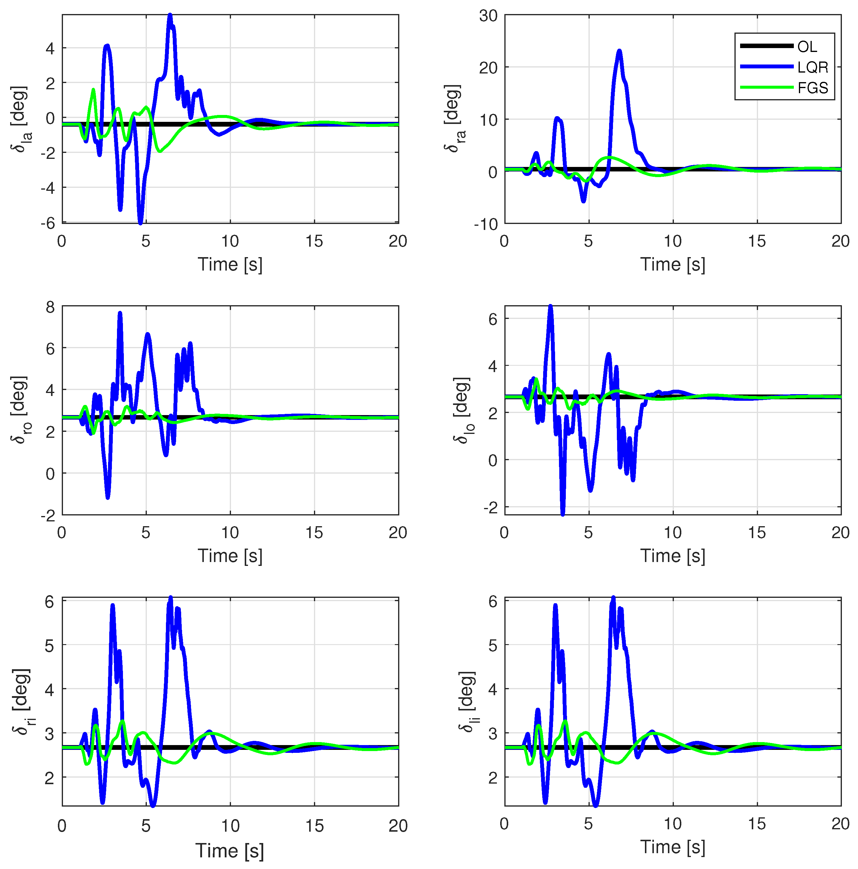
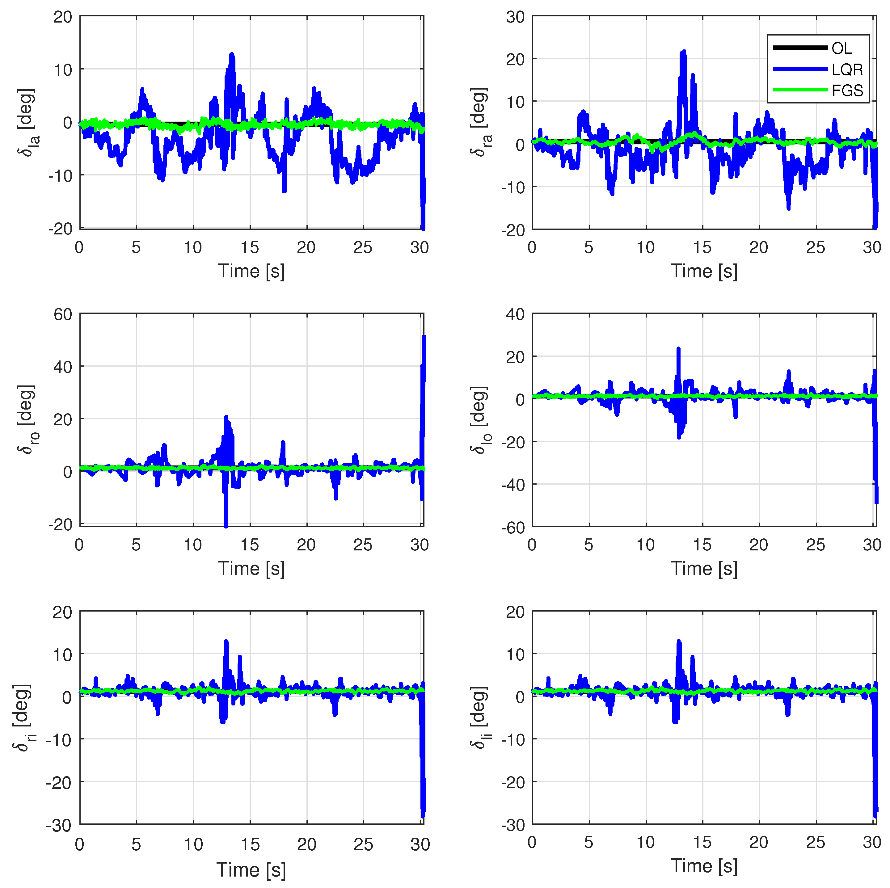
Moreover, actuation system elements make up the control inputs of the aircraft: the elevons, the ailerons, and the electric motors, all of which can be independently controlled. Figure 5 shows the corresponding nomenclature of each control input for the six-meter-san ITA X-HALE aircraft.

Therefore, for the six-meter-span ITA X-HALE, the linear model comprises $n=352$ states: 12 from rigid-body motion; 83 from rigid-body and control-surface aerodynamic lag states; 58 from elastic states; and 199 from aeroelastic aerodynamic lag states. Also, the model presents a total of $m=11$ control input variables, whose disturbances around the equilibrium flight conditions are given as follows:

$$\begin{array}{c}\hfill {\mathit{u}}_{\mathit{ctrl}}={\left[{\delta }_{li}{\delta }_{ri}{\delta }_{lo}{\delta }_{ro}{\delta }_{la}{\delta }_{ra}{\eta }_{lo}{\eta }_{li}{\eta }_C{\eta }_{ri}{\eta }_{ro}\right]}^T\end{array}$$

(38)

where ${\mathit{u}}_{\mathit{ctrl}}\in {\mathbb{R}}^{m\times 1}$. The variables corresponding to the control surface deflections are given in degrees, whereas the ones corresponding to the throttle setting of each motor vary from zero to one (full throttle).

All aircraft actuators (Equation (38)) can be independently commanded. However, a couple of command rules mixing the actuators are enforced to reduce the number of gains to be determined once we can assume that the aircraft is nearly symmetric with respect to the $xz$ plane. In this mixing, it was defined that the inner elevons ${\delta }_{li}$ and ${\delta }_{ri}$ operate symmetrically as elevators (${\delta }_{li}={\delta }_{ri}$), and the outer elevons ${\delta }_{lo}$ and ${\delta }_{ro}$ operate anti-symmetrically (${\delta }_{li}=-{\delta }_{ri}$). The outer electric motors are used differentially to generate yawing motion (${\eta }_C-({\eta }_{lo}+{\eta }_{li})=({\eta }_{ro}+{\eta }_{ri})-{\eta }_C$), in substitution of a rudder, while all motors operate together to generate thrust—in this case, the total thrust is due to the sum of all motors (${\eta }_C+{\eta }_{lo}+{\eta }_{li}+{\eta }_{ro}+{\eta }_{ri}$). Finally, the ailerons ${\delta }_{la}$ and ${\delta }_{ra}$ were employed in both symmetric and antisymmetric motions, with the purpose of correcting the shape of the aircraft. Then, the input vector can be rewritten as follows:

$${\mathit{u}}_{\mathit{SAS}}={\left[{\delta }_{elesym}{\delta }_{eleasym}{\delta }_{ailsym}{\delta }_{ailasym}{\delta }_{th}{\delta }_{rd}\right]}^T$$

(39)

where ${\mathit{u}}_{\mathit{SAS}}\in {\mathbb{R}}^{6\times 1}$. The previous assumptions are mathematically represented by the following output matrix restructuring for disturbances around equilibrium:

$$\begin{array}{cc}{\mathit{B}}_{\delta }=[{\mathit{B}}_{\mathbf{1}}+{\mathit{B}}_{\mathbf{2}}⋮{\mathit{B}}_{\mathbf{4}}-{\mathit{B}}_{\mathbf{3}}⋮\hfill & {\mathit{B}}_{\mathbf{6}}+{\mathit{B}}_{\mathbf{5}}⋮{\mathit{B}}_{\mathbf{6}}-{\mathit{B}}_{\mathbf{5}}⋮\hfill \\ & \hfill {\mathit{B}}_{\mathbf{7}}+{\mathit{B}}_{\mathbf{8}}+{\mathit{B}}_{\mathbf{9}}+{\mathit{B}}_{\mathbf{10}}+{\mathit{B}}_{\mathbf{11}}⋮({\mathit{B}}_{\mathbf{10}}+{\mathit{B}}_{\mathbf{11}})-({\mathit{B}}_{\mathbf{7}}+{\mathit{B}}_{\mathbf{8}})]\end{array}$$

(40)

where ${\mathit{B}}_{\mathit{j}}$ represents the j-th column of the matrix $\mathit{B}$, ${\mathit{B}}_{\delta }\in {\mathbb{R}}^{n\times 6}$.

The output ${\mathit{y}}_{\mathit{SAS}}\in {\mathbb{R}}^{8\times 1}$ comprises model outputs such as attitudes and angular velocities, at different points of the wing and close to the aircraft center of gravity (CG). All outputs used are measurements made via the aircraft sensors and available in the flight control system:

$${\mathit{y}}_{\mathit{SAS}}=\left[{\theta }_c{\varphi }_c{p}_c{r}_c(p_r+p_l-2p_c)(p_r-p_l)(r_r+r_l-2r_c)(r_r-r_l)\right]$$

(41)

The rationale for selecting outputs in Equation (41) is as follows: ${\theta }_c$ is considered to measure the SP and phugoid mode effects; ${\varphi }_c$, $p_c$, and $r_c$ are selected to measure the lateral–directional motion. The fifth element of ${\mathit{y}}_{\mathit{SAS}}$ corresponds to a combination of signals to capture the anti-symmetric bending modes, whereas the sixth element captures the symmetric bending motion. Lastly, and similarly, the seventh and eighth signal combinations capture the symmetric and anti-symmetric in-plane modes, respectively.

3.2. Model Reduction

The high order of the ITA X-HALE model is a challenge to most control techniques; therefore, a state-space reduced-order model is appropriate. For this purpose, a residualization technique [31,36] is applied to all the aerodynamic lag states and the modes with frequency above 8 Hz of the nominal model. The resulting reduced linear model (${\mathit{A}}_{\mathit{r}}$, ${\mathit{B}}_{\mathit{r}}$, ${\mathit{C}}_{\mathit{r}}$, ${\mathit{D}}_{\mathit{r}}$) comprises nine rigid-body states of the full model (discarding ignorable variables x, y, and $\psi$), as well as the fourteen elastic modes below 8 Hz:

$${\mathit{x}}_{\mathit{r}}={\left[V\alpha q\theta H\beta \varphi pr{{\mathit{\eta }}_{\mathit{r}}}^T{{\dot{\mathit{\eta }}}_{\mathit{r}}}^T\right]}^T$$

(42)

The maximum and minimum singular values of the multiple-input, multiple-output (MIMO) transfer function matrix from ${\mathit{u}}_{\mathit{SAS}}$ to ${\mathit{y}}_{\mathit{SAS}}$ for both the full-order and the reduced-order models are shown in Figure 6. It is evident that the reduced model preserves essential characteristics of the full model up to 8 Hz. Additionally, in Figure 6, the response above 10 Hz is not accurately represented by the reduced model. However, a controller with adequate stability margins should be able to accommodate this discrepancy. Similar results were verified for all velocities.

4. Numerical Results

To illustrate the proposed method, the approach detailed in Section 2 was implemented on the six-meter-span ITA X-HALE model. However, its reduced version presented in Section 3.2 was used, primarily due to computational constraints associated with model order. The control inputs from Equation (39) and outputs from Equation (41) were selected. For SAS design, the altitude state has been disregarded. Therefore, the linear model employed in the SAS design is represented as follows:

$$\begin{array}{cccc}\hfill & \hfill {\dot{\mathbf{x}}}_{\mathbf{r}}& =& {\mathbf{A}}_{36\times 36}{\mathbf{x}}_{\mathbf{r}}+{\mathbf{B}}_{{\delta }_{36\times 6}}{\mathbf{u}}_{\mathbf{SAS}}\hfill \end{array}$$

(43)

$$\begin{array}{ccc}\hfill {\mathbf{y}}_{\mathbf{SAS}}& =& {\mathbf{C}}_{8\times 36}{\mathbf{x}}_{\mathbf{r}}\hfill \end{array}$$

(44)

The gains were developed according to the flowchart methodology in Figure 4. The first step is to select the design points. Only velocity was selected as the scheduling variable, with intervals of $0.5$ m/s, varying from $12.5$ to $20.0$ m/s. The model was linearized at each of these velocities under straight and level flight conditions.

The selection of design points was guided by the behavior of the poles. It is evident that the majority of poles exhibit satisfactory behavior concerning variations in velocity, as shown in Figure 7. However, the phugoid and spiral modes demonstrate less linear behavior, due to the nonlinearities present in the propulsive model that was based on wind-tunnel data, as presented by Guimarães Neto et al. [22]. To obtain a reliable representation of these modes, velocities of $12.5$, $13.5$, $14.5$, $15.5$, $16.5$, $18.5$, and $20.0$ m/s were chosen, consistent with those depicted in the membership functions of Figure 3. Other methods for selecting design points, such as the one proposed by Al-Jiboory et al. [37], exist but are not within the scope of analysis for this study.

Once the design points have been selected, the next step is to optimize the LQR PI. The minimization was accomplished numerically using a local search algorithm based on the Nelder–Mead simplex method [38]. A good compromise between closed-loop response and demanded actuation energy was obtained for the following choice of weighting matrices:

$$\begin{array}{cc}\hfill \mathbf{Q}& =\left[\begin{array}{cccc}{\mathbf{I}}_{7\times 7}& {\mathbf{0}}_{7\times 1}& {\mathbf{0}}_{7\times 14}& {\mathbf{0}}_{7\times 14}\\ {\mathbf{0}}_{1\times 7}& 0.75& {\mathbf{0}}_{1\times 14}& {\mathbf{0}}_{1\times 14}\\ {\mathbf{0}}_{14\times 7}& {\mathbf{0}}_{14\times 1}& \left({\displaystyle \frac{1}{{\left(i_1^{14}\right)}^2}}\right){\mathbf{I}}_{14\times 14}& {\mathbf{0}}_{14\times 14}\\ {\mathbf{0}}_{14\times 7}& {\mathbf{0}}_{14\times 1}& {\mathbf{0}}_{14\times 14}& \left({\displaystyle \frac{1}{{\left(i_1^{14}\right)}^2}}\right){\mathbf{I}}_{14\times 14}\end{array}\right]\hfill \end{array}$$

(45)

$$\begin{array}{cc}\hfill \mathbf{R}& =diag\left({\displaystyle \frac{1}{{15}^2}}{\displaystyle \frac{1}{{15}^2}}{\displaystyle \frac{1}{{15}^2}}{\displaystyle \frac{1}{{15}^2}}{\displaystyle \frac{1}{0.{02}^2}}{\displaystyle \frac{1}{0.1^2}}\right)\hfill \end{array}$$

(46)

The Q matrix was chosen as an identity matrix for the rigid body states, with a reduction in weighting for r. The elastic modes were weighted to exert a more significant influence on the lower-frequency modes and a lesser impact on the higher-frequency modes. This was achieved using the weight ${\displaystyle \frac{1}{{\left(i_1^{14}\right)}^2}}$, where i ranges from 1 to 14, corresponding to the number of elastic states. Regarding the R matrix, Bryson’s rule was applied, assigning a higher weight to the rudder.

Finally, the last step involves applying the LMI presented in Equation (33), which arises from the fuzzy system described in Section 2.2.2. The state-space system considered for the LMI is the closed-loop system with gains determined through LQR PI minimization for each design point. The design variable $\kappa$ is further analyzed in the next section.

4.1. $\kappa$ Stability Analysis

The new design variable $\kappa$ is incorporated into the second step outlined in Section 2.5. To assess its impact on stability enhancement, a range of $\kappa$ values, spanning from ${10}^5$ to ${10}^{-10}$, was systematically applied to the LMI set.

Following the application of LMI on top of the LQR design, the disk margin performance between LQR and LMI for different values of $\kappa$ is compared and calculated according to Lavretsky and Wise [39]. As illustrated in Figure 8, the LQR design leads to instability at $13.5$ m/s, exhibiting an overall poor margin with the entire range below $4.5$ dB. Conversely, the methodology proposed for gain design reveals that higher values of $\kappa$ fail to stabilize the entire range, and with the highest value, the margins are even worse than the pure LQR design. However, as the value of $\kappa$ decreases, stability margins substantially increase, with the best result achieved when $\kappa$ is equal to ${10}^{-3}$. With an examination of the sum of the root mean square (RMS) values of the approximation described in Equation (31), presented in Figure 9, it is evident that, for this value, the approximation converges close to zero and achieves an almost steady value for smaller $\kappa$ values. All solutions for which the RMS value was smaller than 1 achieved good stability margins, indicating that, once the approximation is sufficiently accurate, stability margins increase, and global stability is assured. However, it is essential to note that this $\kappa$ value is problem-specific.

4.2. Nonlinear Simulations

After the stability study, simulations focusing on performance degradation analysis at different points used in the design were evaluated. These nonlinear simulations also aim to show the system performance improvement at intermediate velocities where the LMI described in Equation (33) is considered in the controller design.

The simulations were performed with three different control configurations: open loop, closed loop considering the gain calculated through LQR only, and gains calculated using the methodology outlined in the flowchart in Figure 4, which combines LQR and LMI with $\kappa ={10}^{-3}$, referred to simply as FGS. It is also important to note that, for both the LQR and FGS configurations, gain scheduling was implemented using the same fuzzy membership functions, with normalization as described in Section 2.2.2. Accordingly, the gains designed for each method were weighted by the normalized functions defined in Equation (10).

To assess a scenario where the system experiences disturbance around an equilibrium point, simulations were conducted with vertical and horizontal gusts featuring a one-minus-cosine profile during straight-level flight at $17.0$ m/s. Figure 10, Figure 11, Figure 12 and Figure 13 illustrate the results of a simulation in which the aircraft is perturbed by two lateral and two vertical gusts. These gusts have a maximum amplitude of 3 m/s and are fixed in space, with vertical gusts occurring from 17 to 34 m and 51 to 68 m, and horizontal gusts from 34 to 51 m and 68 to 95 m. These distances were chosen to produce approximately one second of exposure per gust, based on the aircraft’s nominal velocity. The gust amplitude exceeds the levels observed during the flight test campaign in order to emphasize the controller’s effectiveness under more challenging conditions. Vertical and horizontal gusts were applied separately with the intent of exciting the aircraft’s longitudinal and lateral modes independently.

Figure 10 presents rigid body outputs. Gains calculated using only LQR demonstrate commendable performance, particularly in the context of lateral–directional motion, exhibiting high attenuation for both $\beta$ and ${\varphi }_c$. The controller that combines both techniques exhibits the best results for longitudinal motion, displaying smaller variations in ${\theta }_c$ and $q_c$. This superior performance is further evident in the RMS values in

Table 1. The RMS values of rigid body outputs during straight flight at a velocity of 17.0 m/s, under the influence of vertical and horizontal wind gusts, are presented for two distinct output feedback realizations and an open loop.

	Open Loop	LQR	FGS
$V_c$ [m/s]	0.193	0.403	0.434
H [m]	0.365	2.99	1.280
${\theta }_c$ [°]	1.54	1.98	1.34
$q_c$ [°/s]	4.61	5.25	3.63
$\beta$ [°]	4.01	2.10	3.21
$r_c$ [°/s]	1.22	0.68	0.26
${\varphi }_c$ [°]	6.93	3.26	5.65
$p_c$ [°/s]	9.64	6.07	7.13

. However, velocity and altitude have deteriorated due to the increased control energy used in all motors, as indicated by the RMS values in

Table 2. The RMS values of control inputs during straight flight at a velocity of 17.0 m/s, under the influence of vertical and horizontal wind gusts, are presented for two distinct output feedback realizations and an open loop.

	Open Loop	LQR	FGS
${\delta }_{ra}$ [°]	0.000	4.720	0.869
${\delta }_{la}$ [°]	0.000	1.630	0.493
${\delta }_{lo}$ and ${\delta }_{ro}$ [°]	0.000	1.170	0.152
${\delta }_{li}$ and ${\delta }_{ri}$ [°]	0.000	0.850	0.186
${\eta }_{lo}$ and ${\eta }_{li}$ [-]	0.000	0.136	0.105
${\eta }_{ro}$ and ${\eta }_{ri}$ [-]	0.000	0.125	0.102
${\eta }_c$ [-]	0.000	0.128	0.103

.

Now, examining the wingtip outputs in Figure 11, it is evident that the gain calculated through the LMI was able to yield the smallest wingtip displacement ($T_z$), consequently resulting in the lowest RMS value, as shown in

Table 3. The RMS values of wingtip outputs during straight flight at a velocity of 17.0 m/s, under the influence of vertical and horizontal wind gusts, are presented for two distinct output feedback realizations and an open loop.

	Open Loop	LQR	FGS
$T_{zl}$ [m]	0.023	0.157	0.022
$T_{zr}$ [m]	0.033	0.206	0.025
$p_{lwt}$ [°/s]	10.00	10.40	7.23
$p_{rwt}$ [°/s]	9.26	10.50	6.80
$r_{lwt}$ [°/s]	1.25	0.90	0.35
$r_{rwt}$ [°/s]	1.30	1.41	0.53
${\eta }_{zlwt}$ [g]	0.168	0.194	0.171
${\eta }_{zrwt}$ [g]	0.174	0.172	0.140

. The results for $r_{wt}$, both left and right, exhibit the most significant attenuation in the FGS design and are associated with wing in-plane motion. Conversely, the LQR-only design resulted in substantial wing displacements and, notably, the poorest outcome for the rates.

Concerning control energy, as depicted in Figure 12 and Figure 13, and highlighted in Table 2, the gains calculated with FGS exhibited superior performance, utilizing less control effort compared to the LQR. This is evident for both control surfaces and motors. Table 2 illustrates the RMS values. Although the physical limits were exceeded by the motors, the FGS design performed better in this regard.

Finally, the controller’s performance was analyzed when the aircraft was exposed to a von Kármán wind turbulence as an external disturbance. Results in the same manner as the results shown above are presented in Figure 14, Figure 15, Figure 16 and Figure 17, demonstrating the system’s response under more realistic and challenging conditions. The turbulence was used to simultaneously excite all motion axes, and its intensity was intentionally set higher than typical flight conditions to highlight the controller’s performance. Additionally, this scenario induced variations in velocity that crossed below 13 m/s, where the LQR controller becomes unstable, further testing the effectiveness of the proposed method.

The rigid body results in Figure 14 exhibit a similar pattern in terms of attenuations, with the LQR showing a superior response in lateral–directional motion and the FGS outperforming in longitudinal motion. Notably, instabilities are observed in $q_c$ for the LQR design, particularly as the phugoid mode is degenerated and couples with the spiral mode, leading to instability at a flight velocity of $13.0$ m/s. Consequently, whenever the aircraft traverses this unstable region, the LQR design exhibits an inappropriate response, causing the simulation to crash after 30 s. In the other two instances when the aircraft passes through the unstable region, the aircraft recovers because the turbulence itself increases the aircraft’s velocity.

Examining both Figure 14 and

Table 4. The RMS values of rigid body outputs during straight flight at a velocity of 14.5 m/s, under the influence of a von Kármán wind turbulence, are presented for two distinct output feedback realizations and an open loop.

	Open Loop	LQR	FGS
$V_c$ [m/s]	0.812	0.917	0.577
H [m]	4.04	4.80	5.10
${\theta }_c$ [°]	4.04	3.84	1.93
$q_c$ [°/s]	6.89	9.44	4.53
$\beta$ [°]	5.78	2.89	4.51
$r_c$ [°/s]	1.33	1.21	0.27
${\varphi }_c$ [°]	7.72	2.06	5.64
$p_c$ [°/s]	9.66	3.50	6.59

, it is evident that the highest attenuation was achieved through the controller designed with LQR for lateral motion. However, the FGS design can ensure stability at intermediary points while still offering some improvement over the open-loop response.

The wingtip outputs depicted in Figure 15 reveal a greater attenuation in wingtip displacement for the controller that combines LQR and LMI methods compared to the LQR-only controller. This is attributed to the more pronounced aileron deflections for the LQR design, as observed in Figure 16, resulting in a greater aerodynamic force on the ailerons and, consequently, in wingtip displacement. While Figure 15 may not clearly indicate whether the FGS controller outperforms the open-loop one,

Table 5. The RMS values of wingtip outputs during straight flight at a velocity of 14.5 m/s, under the influence of a von Kármán wind turbulence, are presented for two distinct output feedback realizations and an open loop.

	Open Loop	LQR	FGS
$T_{zl}$ [m]	0.041	0.138	0.034
$T_{zr}$ [m]	0.047	0.142	0.039
$p_{lwt}$ [°/s]	10.20	8.86	6.98
$p_{rwt}$ [°/s]	10.20	9.22	6.78
$r_{lwt}$ [°/s]	1.66	1.78	0.82
$r_{rwt}$ [°/s]	1.85	2.42	0.84
${\eta }_{zlwt}$ [g]	0.284	0.424	0.263
${\eta }_{zrwt}$ [g]	0.206	0.365	0.164

demonstrates that the FGS controller exhibited better performance for all outputs.

The FGS design demonstrated lower expended control energy, consistent with the previous simulation. In terms of motor usage, as shown in Figure 17, the FGS was able to stay within the limits, while the LQR exceeded the limits on several occasions. This is particularly crucial for HALE aircraft, where the control of energy usage is critical. The results presented in

Table 6. The RMS values of control inputs during straight flight at a velocity of 14.5 m/s, under the influence of a von Kármán wind turbulence, are presented for two distinct output feedback realizations and an open loop.

	Open Loop	LQR	FGS
${\delta }_{ra}$ [°]	0.000	4.990	0.696
${\delta }_{la}$ [°]	0.000	4.800	0.520
${\delta }_{lo}$ and ${\delta }_{ro}$ [°]	0.000	3.530	0.293
${\delta }_{li}$ and ${\delta }_{ri}$ [°]	0.000	1.910	0.262
${\eta }_{lo}$ and ${\eta }_{li}$ [-]	0.000	0.204	0.096
${\eta }_{ro}$ and ${\eta }_{ri}$ [-]	0.000	0.191	0.098
${\eta }_c$ [-]	0.000	0.196	0.097

underscore a significant improvement in this regard.

5. Conclusions

An output feedback gain scheduling approach based on fuzzy logic has been proposed in this paper to solve stability issues in intermediate regions to those chosen for the linear controller design. The approach combines closed-loop performance improvement via LQR and stability enforcement in the whole flight envelope through the Lyapunov direct method. The proposed approximation for the output feedback demonstrates effectiveness. As $\kappa$ decreases, the approximation tends toward zero, ensuring overall stability.

Results comparing the proposed approach with traditional interpolation-based gain scheduling techniques showed that the present technique achieved overall better performance, smoother closed-loop responses, and higher and more constant gain and phase margins in the entire velocity envelope. Thus, there is enormous potential to reduce the time necessary in control law development without the need to run several simulations (e.g., Monte-Carlo simulations) to look for stability issues in the entire envelope.

In this paper, the LQR method was selected to optimize the controller for performance. Nevertheless, it is worth noting that other techniques can be employed in this step of the process.