Research on Aircraft Control System Fault Risk Assessment Based on Composite Framework

Abstract

The air transportation system is composed of multiple elements and belongs to a complex socio-technical system. It is difficult to assess the risk of an aircraft fault because it could constantly change during operation and is influenced by numerous factors. Although traditional methods such as Failure Mode, Effects, and Criticality Analysis (FMECA) and Fault Tree Analysis (FTA) can reflect the degree of fault risk to a certain extent, they cannot accurately quantify and evaluate the fault risk under the multiple influences of human factors, random faults, and external environment. In order to solve these problems, this article proposes a fault risk assessment method for aircraft control systems based on a fault risk composite assessment framework using the Improved Risk Priority Number (IRPN) as the basis for the fault risk assessment. Firstly, a Bayesian network (BN) and Gated Recurrent Unit (GRU) are introduced into the traditional evaluation framework, and a hybrid prediction model combining static and dynamic failure probability is constructed. Subsequently, this paper uses the functional resonance analysis method (FRAM) by introducing a risk damping coefficient to analyze the propagation and evolution of fault risks and accurately evaluate the coupling effects between different functional modules in the system. Finally, taking the fault of a jammed flap/slat drive mechanism as an example, the risk of the fault is evaluated by calculating the IRPN. The calculation results show that the comprehensive failure probability of the aircraft control system in this case is 3.503 × 10⁻⁴. Taking into account the severity, the detection, and the risk damping coefficient, the calculation result of IRPN is 158.00. According to the classification standard of the risk level, the failure risk level of the aircraft belongs to a controlled risk, and emergency measures need to be taken, which is consistent with the actual disposal decision in this case. Therefore, the evaluation framework proposed in this article not only supports a quantitative assessment of system safety and provides a new method for fault risk assessments in aviation safety management but also provides a theoretical basis and practical guidance for optimizing fault response strategies.

1. Introduction

Civil aircraft is one of the important components of air transportation, and ensuring flight safety is the primary requirement for the operation of civil aircraft. According to the International Civil Aviation Organization’s “State of Global Aviation Safety” report, the total number of aviation accidents increased by 33.3% from 2021 to 2022. In 2022, the global average flight accident rate increased by 6.3% year-on-year to 2.05 accidents per million flights. Accidents related to the aircraft control system accounted for 14.3% of all fatal accidents [1,2,3]. The aircraft control system, which plays a crucial role in ensuring flight safety, faces significant risks due to the complexity of the system and the variability of environmental conditions. Therefore, predicting and evaluating the failure risk of aircraft control system are necessary in order to improve flight safety.

The failure risk assessment of the aircraft control system aims to analyze failure risk information, predict the probability of a failure occurrence, determine the causes of failure, analyze potential hazards and losses, and evaluate the risk level of the failure. The fault risk assessment methods include Failure Modes, Effects, and Criticality Analysis (FMECA), Fault Tree Analysis (FTA) [4,5], and Hazard and Operations Study (HAZOP), among which the FMECA method is the most commonly used. The U.S. military introduced FMECA in the 1940s and issued “MIL-P-1629” in 1949, taking FMECA as the safety standard [6]. Up to now, FMECA has been widely used in various industrial products, including the power system, aviation, and aerospace sectors.

This method is an inductive, bottom-up analysis approach that examines all potential failure modes in a system and their possible impacts on the system, and categorizes each failure mode according to its severity and probability of occurrence. It provides an effective way to identify and analyze potential failure modes in aircraft systems [7,8,9].

However, the traditional FMECA method has some limitations in assessment accuracy. In the FMECA method, the Risk Priority Number (RPN) is an important metric used to determine the failure effect and priority of potential issues, whose value is equal to the product of severity (S), detectability (D), and occurrence (O). Therefore, the result of the RPN can only be a finite number of discrete integers, which only represents the comparative order of risk levels and does not reflect the actual magnitude of the risk [10,11]. Moreover, the assignment of each item in the RPN is based on a subjective evaluation and cannot be accurately quantified. As a result, combining other quantitative assessment methods is necessary to comprehensively analyze and evaluate the risk of fault.

As a commonly used quantitative analysis method, FTA is often introduced in combination with FMECA. FMECA is a single-factor analysis method that primarily focuses on the impact of a single fault mode on the system. FTA can analyze the combined effects of multiple fault factors on the system, making it more suitable for a complex system analysis. The combination of FMECA and FTA can significantly increase the effectiveness of the risk assessment and is widely used in the field of aviation safety [12,13,14]. However, this method still cannot fully clarify the impacts of human and environmental factors on risk [15].

In order to solve the above-mentioned similar problems, in some studies, according to the mapping relationship between FTA and Bayesian network, the Bayesian network model based on the FTA is constructed. The Bayesian network model is the most effective theoretical model in the field of uncertain knowledge expression and reasoning, and it has obvious advantages in dealing with uncertain information. Using a BN, we can not only establish a comprehensive risk model considering many factors, such as organization, personnel, and the environment, but also effectively complete the risk analysis of uncertain problems with incomplete data and obtain more objective quantitative analysis results [16,17,18]. In recent years, with the successful application of the Bayesian network in many fields [19,20,21,22], aviation safety researchers have gradually applied the Bayesian network to aircraft risk assessments.

In the above methods, the failure probability is usually a static result calculated using historical data under experimental conditions. Earlier, due to limitations in the frequency of updates and data quality of ground-to-air communication networks, it was reasonable to use this static result to characterize the probability of failures. However, the failure probability actually changes over time and should be continuously updated based on the operational state data of the control system. With the continuous improvement of ground-to-air communication technology, the demand for the dynamic prediction of fault probability has become urgent. This article proposes an improved hybrid prediction model to increase the accuracy of the fault probability calculation [23,24]. This model consists of a static prediction module and a dynamic prediction module. The static prediction module adopts a composite architecture that integrates FMECA, FTA, and BN algorithms, which can be used to quantitatively calculate the basic failure risk probability of the flight control system. The dynamic prediction module introduces the GRU neural network model [25], focusing on analyzing the operational data characteristics of the control system and a rolling forecast of the incremental probability of a failure occurrence.

In addition to identifying and analyzing faults, the propagation and evolution of risks within the system, as well as their impacts on the occurrence of accidents, are also worthy of attention. To increase the dimension of the failure risk assessment, deeply analyze the risk evolution process after a failure occurrence, and quantitatively assess the risk level, the risk damping is introduced as one of the key risk assessment parameters into the traditional RPN model in this study. The concept of risk damping originates from the functional resonance analysis method (FRAM) that is widely used to analyze complex socio-technical systems, which characterizes the evolution of risk in a system. For a long time, FRAM has been widely used in the investigation and analysis of aviation accidents, such as the Comair flight accident [26] and the Alaska Airlines flight 261 accident [27]. This method is not limited to system structure decomposition and causal factor analysis. It views accidents as essentially sudden changes in the normal operation of the system, emphasizing that accidents should be explained from the perspective of the entire system and avoiding treating accidents as ordered occurrences of individual events or the hierarchical stacking of potential factors [28]. By dividing the entire system into different functional modules, it provides the possibility of studying the whole system [29]. This paper evaluates the functional variability of the system in terms of time and accuracy, analyzes the upstream and downstream coupling resonance in the risk evolution process, and sets the risk damping coefficient under specific failure modes to accurately locate the causes of accidents and quantify the degree of risk propagation.

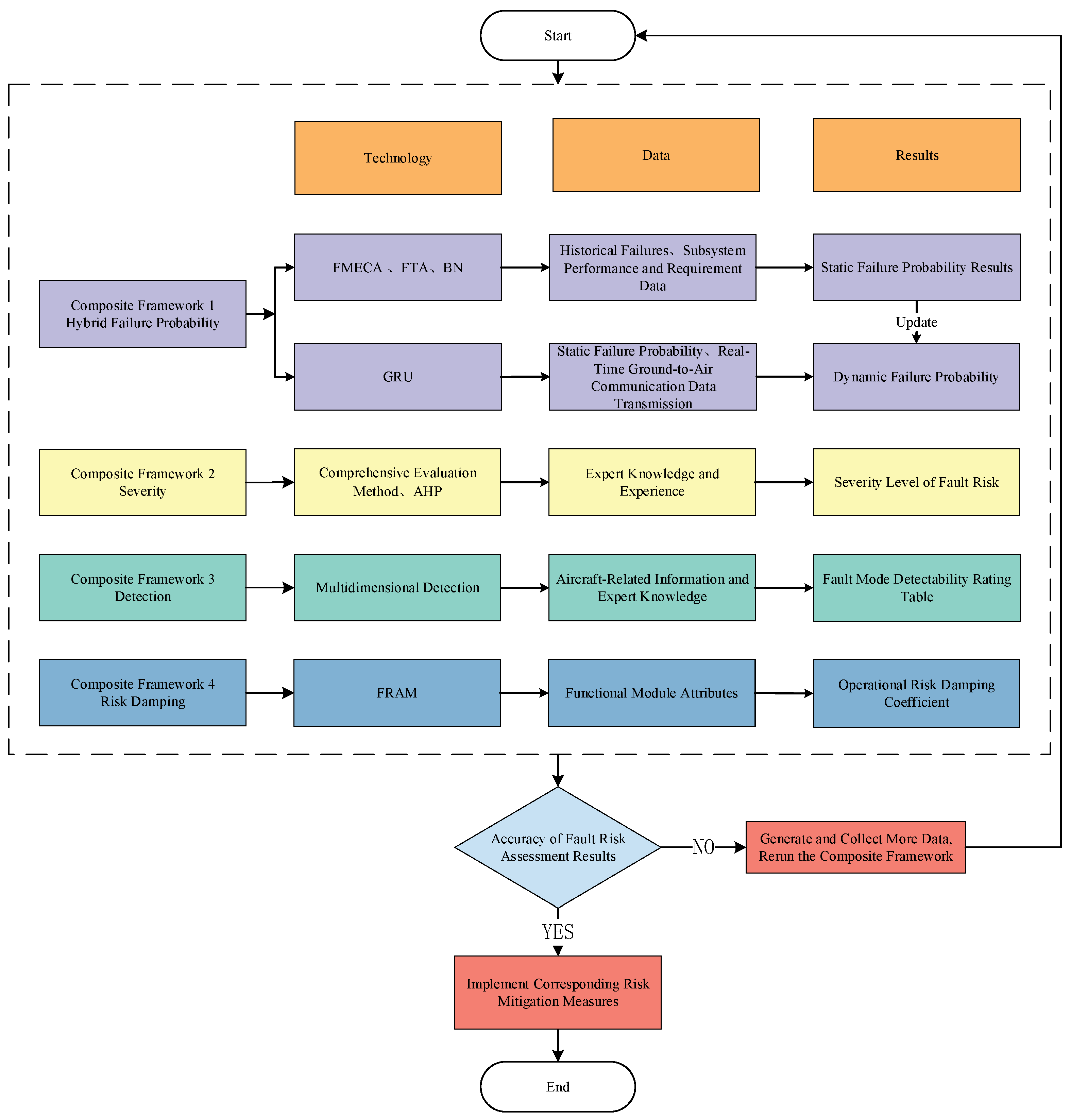
This paper proposes a fault risk assessment method that integrates static–dynamic information and a multi-source data-driven and functional propagation mechanism analysis, and applies it to the quantification of the fault risk in aircraft control systems. Compared with existing research, this method has significant innovations in the following three aspects: (1) By combining FMECA and FTA, this paper first establishes a bidirectional inference model for the fault risk, and then integrates Bayesian networks to quantitatively analyze the impacts of human and environmental factors. This method significantly improves the accuracy of the static fault probability calculation. (2) This article introduces deep learning algorithms to construct a dynamic calculation model for the fault probability using aircraft operation data, and then combines the results of the static fault probability calculation to comprehensively quantify the fault probability. (3) It proposes a fault risk composite assessment framework based on IRPN, which integrates the risk evolution theory based on FRAM into traditional risk parameter calculations such as severity, detectability, and occurrence effectively, addressing the shortcomings of existing fault risk assessment models.

The structure of this paper is as follows. Section 2 introduces the proposed fault risk composite assessment framework. Section 3 elaborates on the theory and procedures of the proposed method. Section 4 discusses cases used to validate the applicability and accuracy of the model. Section 5 summarizes the above research content.

2. Design of the Composite Framework for the Fault Risk Assessment

The risk of aircraft control system failure is defined as the comprehensive measurement of the probability of system component failure or performance degradation induced by various internal or external factors during normal operation, and the actual harm that may be caused.

The triggers of a failure risk are numerous and complex. Furthermore, there is an uncertain evolutionary trend from the formation of risks to the triggering of accidents. Usually, traditional risk priority numbers are used to evaluate risks by calculating the product of three factors, failure occurrence, severity, and detectability, with the aim of obtaining risk assessment results through an overall comprehensive evaluation. However, this method is subjective and cannot accurately assess the risks of serious faults with a low probability of occurrence. In addition, the calculation result of the risk priority number is discrete and limited to a finite set of integers. To increase computational accuracy, this paper constructs a risk assessment composite framework based on an improved RPN. This framework introduces a risk damping coefficient, uses a fuzzy comprehensive evaluation method to assess the severity of faults, establishes a mixed probability model to calculate the occurrence of faults, and constructs a multidimensional evaluation system to quantify the detectability. The composite framework for fault risk assessment is shown in Figure 1.

(1) Step 1: Use the FMECA method to analyze the failure modes, causes, and impacts of various components of the aircraft control system [30,31]. By introducing the fault tree method, this article derives system component failures in reverse based on the Mean Time Between Failures (MTBF) and calculates their failure probabilities. This method obtained the theoretical failure probability of the system, but did not consider other key factors such as operational failures caused by maintenance personnel errors, bird strikes, and the impacts of harsh environmental conditions such as thunderstorms.

Therefore, this article constructs a fault mixed probability calculation model that integrates static and dynamic characteristics. The model consists of two parts. In the first part, a static fault inference model based on Bayesian networks was constructed. This model defines the relationships between nodes, directed edges, and fault probabilities based on expert knowledge and historical fault data. Through data training, it calculates the probability of faults occurring under the influence of human and environmental factors. In the second part, based on real aircraft operation and fault simulation platform data, this paper uses GRU neural network method to predict the probability of aircraft faults.

(2) Step 2: After dividing the severity of faults into three characteristic parameters, unsafe loss, equipment damage, and maintenance cost, this paper uses Analytic Hierarchy Process (AHP) to allocate weights and adopts a fuzzy comprehensive evaluation method to solve the uncertainty problem in the expert scoring process [32].

(3) Step 3: Based on the pilot’s quick reference handbook, aircraft manual, maintenance manual, ground support manual, and expert knowledge and experience, a fault detection level allocation rule is established from the two dimensions of recognition speed and diagnostic accuracy of fault detection methods to determine the detectability level of specific faults.

(4) Step 4: In order to deeply analyze the risk evolution process after the occurrence of faults and quantitatively evaluate the risk level of faults, the functional resonance analysis method applicable to socio-technical systems was introduced. This method evaluates the system’s functional variability based on changes in time and accuracy, analyzes the upstream and downstream coupling resonance during the risk evolution process, and quantifies the degree of risk propagation by setting risk damping coefficients in specific fault modes, providing a computational basis for the composite framework of fault risk assessment.

(5) Step 5: Based on the fault risk composite framework evaluation model, the comprehensive fault risk index is calculated, which can accurately quantify the risk level of fault modes in aircraft operation and quantitatively analyze the tendency of unsafe events caused by faults.

3. Implementation of Key Technologies

The FMECA method summarized in engineering practice adopts the risk priority number (RPN) as the risk assessment index, which can discretely sort and calculate the fault risk. However, traditional RPNs do not consider the mapping relationship from faults to actual operational consequences and lack an analysis of the impact on risk evolution.

This paper designs a composite fault risk assessment framework based on the Improved Risk Priority Number (IRPN) index. This framework consists of risk indices such as failure occurrence, severity, detectability, and risk damping, and its calculation formula is shown in Equation (1):

$$\mathrm{IRPN}=O\times S\times D\times W$$

(1)

where $O$ represents a failure occurrence, $S$ represents severity, $D$ represents detectability, and $W$ represents risk damping.

In order to quantify and classify the risk of failure of key components in aircraft control systems, this paper establishes a risk level classification standard for the IRPN calculation results based on the FMECA process [33,34], which is shown in

Table 1. Risk level classification standard for the IRPN.

Risk Level	Range	Description
Negligible Risk	IRPN < 90	The risk of this level is very low, indicating that the probability of a failure occurrence during operation is small, or even if it occurs, the impact on overall safety can be ignored.
Controlled Risk	90 ≤ IRPN < 160	The controllable risk of this level indicates that there is a certain possibility of a malfunction occurring that may have a certain impact on the system, but the risk can be reduced and mitigated through appropriate control measures.
High Risk	IRPN ≥ 160	The risk at this level is relatively high, indicating a high possibility of malfunction, and once it occurs, it may pose a significant threat to flight safety and even lead to catastrophic accidents.

. This standard was derived by reviewing and analyzing the relevant literature and incorporating historical data provided by several major international airlines, as well as the opinions of maintenance experts.

This risk level classification standard refers to the application experience of the traditional FMECA analysis method and has been appropriately improved to meet the specific needs of flight control systems, especially considering the impacts of environmental and human factors on risks, thereby improving the accuracy and credibility of the assessment results.

Specifically, this paper collected 131 typical approach-phase failure events from 9 global airlines between 2018 and 2023 (the data covers 78% of mainstream civil aviation aircraft models). The data includes:

Event investigation reports issued by civil aviation authorities (such as EASA and CAAC), including descriptions of failure modes and consequence classification; historical maintenance records from airline maintenance databases; functional architecture diagrams; and Fault Tree Analysis (FTA) reports provided by component manufacturers.

The IRPN values calculated for the above events range from 37 to 665. To classify the risk levels into three tiers, this study employs a combined approach of clustering analysis and expert experience calibration. Based on the data distribution characteristics, significant differences in data aggregation were identified near the values of 90 and 160. By examining the risk consequence differences across clusters, it was found that 100% of events in Cluster 3 resulted in approach go-arounds or emergency procedure activations, while only 6.7% of events in Cluster 1 required additional crew intervention. This indicates that the classification results are highly correlated with the actual risk levels.

3.1. Assessment of Occurrence

The paper constructs a hybrid probability model consisting of FMECA, FTA, and Bayesian methods to reason the potential failure probabilities of the system and components. The FMECA method focuses on studying all potential failure modes related to the analyzed subsystem, while FTA evaluates and calculates the overall steady-state failure rate of the subsystem, and characterizes the logical relationship between subsystem failure events and corresponding component failure modes [35]. After identifying the failure modes, a Bayesian-based inference model is used to analyze the coupling relationships between the component failures of the subsystem and external environmental, human, and other factors.

FMECA is a systematic method used to identify and assess potential failure modes in systems, products, or processes. It involves a systematic analysis of the system or components, organizing agreed hierarchies, and exploring the failure probabilities of the most fundamental elements [36].

Fault Tree Analysis (FTA) is a qualitative and quantitative analysis method represented as a tree structure, including top events, basic events, and logic gates. Using the FMECA analysis results, a FTA topology diagram is constructed with the flight control subsystem as the top event and the system component failure mode as the bottom event. The failure probability of bottom events is calculated using Equation (2):

$${\lambda }_K={\displaystyle \frac{N_K}{{\displaystyle \sum h}}}$$

(2)

where ${\lambda }_k$ is the failure rate of failure mode k; $N_k$ is the number of failures of failure mode k during a given period; and ${\sum }_h$ is the cumulative operating time of failure mode k.

After calculating the failure probabilities of various failure modes, the overall failure probability W of the system can be calculated using the following formula:

$$O=1-{\displaystyle \prod _{i=1}^n(1-O_i)}$$

(3)

where $O_i$ represents the probability of the i-th failure mode.

The probability of system and component failures is not only related to their own performance but is also closely related to specific operating environments and human factors. In order to fully consider the influences of these factors on the fault prediction, this paper adopts the Bayesian network method.

The Bayesian network is a probabilistic graph model used to model conditional dependencies between random variables. The conditional dependency between random variables can be expressed as follows:

$$O(\mathrm{A}|\mathrm{B})={\displaystyle \frac{O(\mathrm{B}|\mathrm{A})\cdot O\left(\mathrm{A}\right)}{O(\mathrm{B})}}$$

(4)

where $O(\mathrm{A}|\mathrm{B})$ is the posterior probability of event A given event B; $O(\mathrm{B}|\mathrm{A})$ is the likelihood of event B given event A; $O\left(\mathrm{A}\right)$ is the prior probability of event A; and $O\left(\mathrm{B}\right)$ is the total probability of event B. A Bayesian network consists of nodes (representing random variables) and directed edges (representing dependencies between variables). For a Bayesian network defined on $X_1,X_2,\dots ,X_n$, its joint probability distribution can be represented as the product of the conditional probability distributions:

$$O(X)={\displaystyle \prod _{\mathrm{i}}{O}_{\mathrm{i}}(X_i|O_g(X_i))}$$

(5)

where $O_g(X_i)$ is the parent node of node $X_i$ and $O_{\mathrm{i}}(X_i|O_g(X_i)$ is the conditional probability distribution table for node $X_i$.

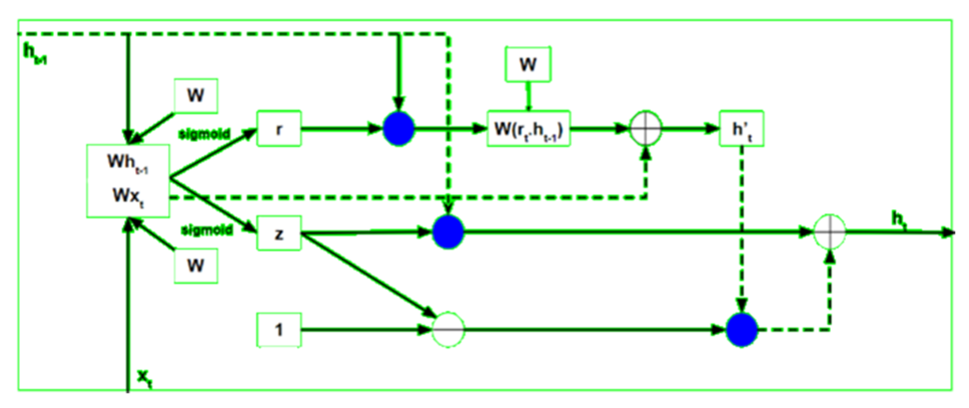
Due to the neglect of external conditions during aircraft operation, static models have certain limitations in terms of failure probability. We need to build a predictive model that can effectively capture the temporal characteristics of data during system operation. Therefore, this article further proposes a dynamic fault inference model based on a Gated Recurrent Unit (GRU) neural network.

GRU is an improved version of the Recurrent Neural Network (RNN) and a simplified variant of Long Short-Term Memory (LSTM) networks [37,38]. The GRU model adopts a unique gating design that can adaptively selectively forget and update information in the sequence, fully mining the long-term dependencies of the sequence data. Compared to traditional RNN method, the GRU model can better address issues such as vanishing and exploding gradients, while also reducing the risk of overfitting. Figure 2 shows the structure of the GRU unit.

The GRU takes two inputs as vectors: the current input Xt and the previous hidden state h_t−1. At each timestamp t, it takes an input Xt and the hidden state h_t−1 from the previous timestamp t − 1. Later it outputs a new hidden state ht, which again is passed to the next timestamp.

There are three gates in a GRU: the Reset Gate, Update Gate, and Reset Gate. It performs an element-wise multiplication (like a dot product for each element) between the current input and the previous hidden state vectors. An activation function (a function that transforms the values) is applied element-wise to each element in these parameterized vectors. This activation function typically outputs values between 0 and 1, which will be used by the gates to control information flow.

Based on the methods described above, the composite fault probability level intervals are defined. The detailed breakdown of these intervals is provided in

Table 2. Fault probability level intervals.

Level	Failure Mode Occurrence Likelihood	Reference Probability Range
1	Very Low (Unlikely to Occur)	$O<{10}^{-6}$
2	Low (Seldom Occurs)	${10}^{-6}\le O<2\times {10}^{-5}$
3	Moderate (Occasionally Occurs)	$2\times {10}^{-5}\le O<5\times {10}^{-3}$
4	High (Frequently Occurs)	$5\times {10}^{-3}\le O<{10}^{-1}$
5	Very High (Constantly Occurs)	$O\ge {10}^{-1}$

, which helps in quantifying the fault levels.

3.2. Evaluation of Failure Severity and Detectability

3.2.1. Fuzzy Comprehensive Evaluation Method

Failure severity is an important indicator in assessing failure risks, primarily focusing on the extent of harm and impact caused by the occurrence of the failure. To accurately assess the severity of different failure modes, this indicator is further subdivided into three evaluation characteristic factors: safety damage, equipment loss, and maintenance cost. Due to the lack of historical data in the engineering field and the particularity of risk characterization factors themselves, in an actual assessment, it is usually necessary to rely on expert experience to determine the hazard based on the established assessment level. In order to make the evaluation results more accurate and in line with the actual situation, fully considering the importance differences between evaluation factors, the Analytic Hierarchy Process (AHP) method is used to weight the factors to characterize the importance between different factors. Based on the obtained weight results, the fuzzy comprehensive evaluation method is used to quantitatively evaluate the severity of the fault.

(1) Establishing the factor set and evaluation set. The three factors related to the fault severity assessment constitute the factor set U:

$$U=\left\{u_1,u_2,u_3\right\}$$

(6)

where $u_i$ represents the i-th influencing factor.

The evaluation set V represents all possible outcomes of the influencing factors on the evaluation object:

$$V=\left\{\begin{array}{cccccc}{v}_1& v_2& \dots & v_j& \dots & v_n\end{array}\right\}$$

(7)

where $V_j$ represents the j-th level of the evaluation object.

(2) Constructing the factor evaluation matrix. Before a comprehensive evaluation, single-factor evaluations are conducted. Let the degree of membership of the i-th factor ui to the j-th evaluation level $V_j$ be n_ij, forming the single-factor evaluation set for $u_i$. An expert evaluation group of x members assigns evaluation levels to each influencing factor. If x_ij members out of x assign $u_i$ to $V_j$, the evaluation set for $u_i$ is

$$\left\{\begin{array}{l}{n}_i=\left[\begin{array}{cccc}{\displaystyle \frac{x_{i1}}{x}},& {\displaystyle \frac{x_{i2}}{x}},& \dots ,& {\displaystyle \frac{x_{in}}{x}}\end{array}\right]\\ {\displaystyle \sum _{j=1}^m{n}_{ij}=1}\end{array}\right\}$$

(8)

The evaluation sets for all factors form the evaluation matrix N

$$\begin{array}{l}N={\left[\begin{array}{cccc}{n}_1& n_2& \dots & n_n\end{array}\right]}^T\\ =\left[\begin{array}{cccc}{n}_{11}& n_{13}& \dots & n_{1m}\\ n_{21}& n_{22}& \dots & n_{2m}\\ ⋮& ⋮& \ddots & ⋮\\ n_{n1}& n_{n2}& \dots & n_{nm}\end{array}\right]\end{array}$$

(9)

(3) Construction of the weight set for each influencing factor

(1) Analytic Hierarchy Process (AHP).

A judgment matrix is constructed as follows:

$$\mathit{A}=\left[\begin{array}{cccc}{a}_{11}& a_{12}& \dots & a_{1n}\\ a_{21}& a_{22}& \dots & a_{2n}\\ ⋮& ⋮& \ddots & ⋮\\ a_{n1}& a_{n2}& \dots & a_{nn}\end{array}\right]$$

(10)

where a_ij reflects the relative importance of factor u_i compared to u_j, following the criteria in

Table 3. Criteria for constructing the judgment matrix.

Meaning	${\mathit{a}}_{\mathit{i}\mathit{j}}$
Equal Importance	1
Slightly More Important	3
Significantly More Important	5
Strongly More Important	7
Absolutely More Important	9
Intermediate Values	2, 4, 6, 8

. The values in the judgment matrix are determined based on a 1–9-point scale, combined with expert evaluations and literature calibration.

(2) Consistency check

The maximum eigenvalue and corresponding eigenvector of the judgment matrix are calculated. After normalization, the consistency ratio (CR) is computed as follows:

$$CR={\displaystyle \frac{CI}{RI}}$$

(11)

When CR < 0.1, the consistency is acceptable.

(3) Comprehensive fuzzy evaluation

For a specific fault mode k, the comprehensive evaluation matrix B is defined as follows:

$$B_k=A\times N=(b_1,b_2,\dots ,b_m)$$

(12)

where A is the weight set and N is the evaluation matrix, $b_k={\sum }_{i=1}^n{a}_i{r}_{ik}$, $k=1,2,\dots ,n$.

The severity parameter is determined using the maximum membership principle:

$$S={\displaystyle \sum _{k=1}^5{B}_K\times k}$$

(13)

3.2.2. Detectability Level Allocation Rules

Failure detection is one of the critical factors related to civil aviation safety. The timely diagnosis of faults is of great significance for troubleshooting, isolation, and prevention of fault propagation. Therefore, scientifically establishing a unified scoring standard and conducting a reasonable quantitative evaluation of the degree of fault mode detection are necessary to measure the difficulty of detecting potential failure modes. The detectability level allocation rules are shown in Table 3.

During operation, the main failure detection methods for aircraft include airborne warning systems, ground-based remote diagnostics, and pilots’ visual observations. The airborne warning system provides critical fault display and alarm information to pilots by reading the fault codes of the aircraft’s central processing unit. With the support of real-time data links/satellite communication technology, ground-based remote diagnostics and real-time tracking systems can also dynamically diagnose the aircraft’s system status. In addition, some failure modes have significant fault manifestations that can be identified by pilots through manual observation. Therefore, detectability levels can be classified into five levels (1 to 5) based on two dimensions, the speed of fault detection and diagnostic accuracy as shown in

Table 4. Detectability level allocation rules.

Levels	Detectability Definitions	Evaluation Criteria
1	Easy to Detect	The current detection method can accurately detect the fault mode it belongs to, and the results are reliable.
2	Fairly Easy to Detect	The current detection method has a high probability of detecting these faults.
3	May be Detected	The current detection method may detect these faults.
4	Hard to Detect	The current detection methods have difficulty detecting these faults, and the results are unreliable.
5	Undetectable	The current detection method has defects. The fault mode cannot be detected.

, to comprehensively assess the results of each detection method. Subsequently, based on the scores derived from expert evaluations [39], the median of the maximum values from the three detection methods is used as the result of the comprehensive evaluation. This method integrates multi-dimensional information and provides a more detailed evaluation standard.

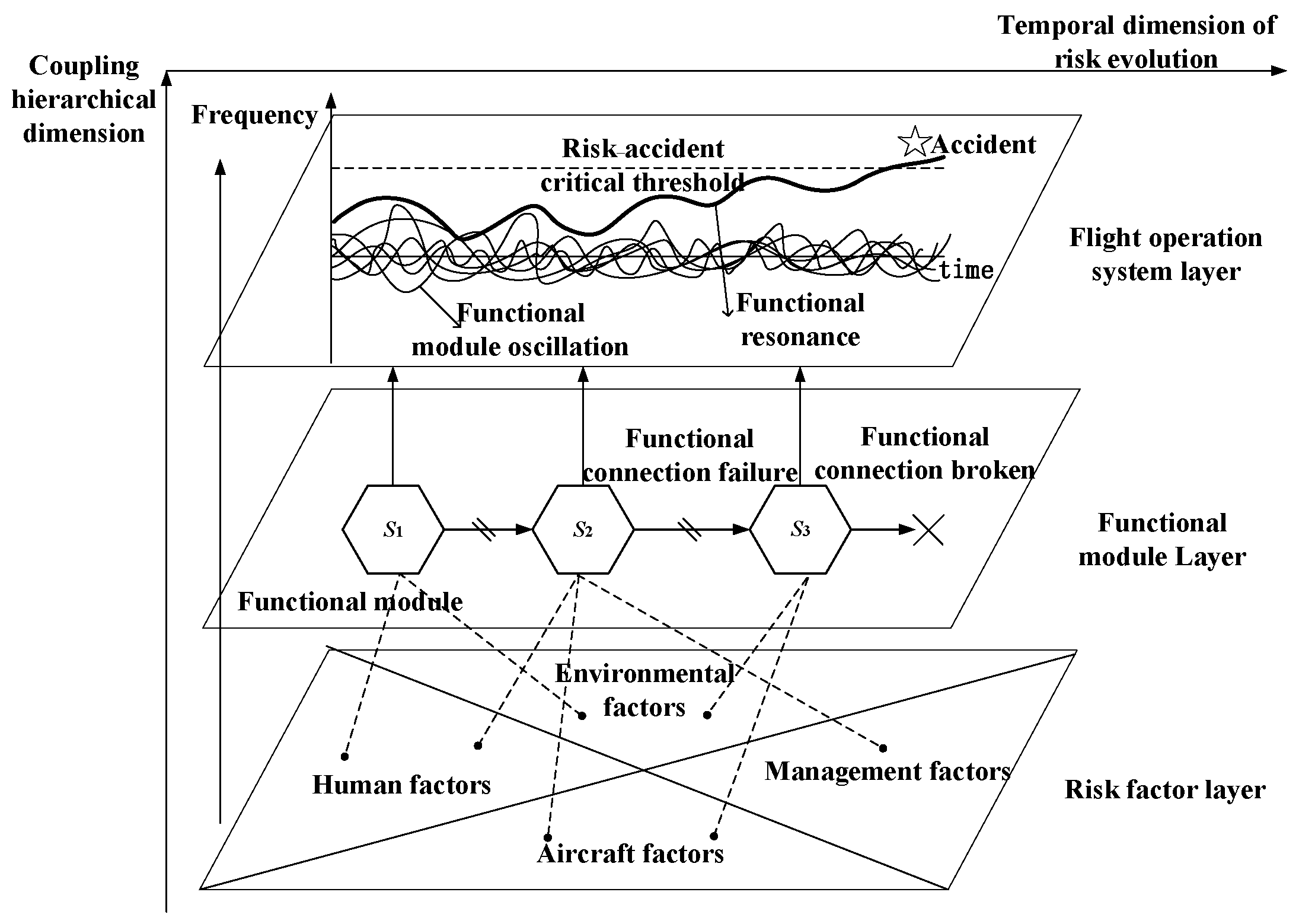
3.3. Functional Resonance Analysis Method

Functional Resonance Analysis Method (FRAM) mainly studies the interrelationships between system functions from the perspective of the functional resonance of the system itself, identifies key weak links from numerous risk factors, and predicts and limits adverse resonance situations in the system. FRAM can perform inductive reasoning and also has deductive reasoning logic, believing that the occurrence of an accident is caused by the failure of a certain functional module in the system, which triggers a series of functional modules to resonate with it [40,41,42,43]. As more and more oscillating functional modules participate in the risk evolution process, once the resonance exceeds the critical threshold of system risk accident, the system may lose control, cause accidents, and result in loss of life and property. Therefore, when studying the risk of aircraft control system failures, in addition to analyzing the failure itself, it is also necessary to consider the series of risk propagation and evolution processes caused by the occurrence of the failure. The risk evolution analysis framework based on the FRAM is shown in Figure 3.

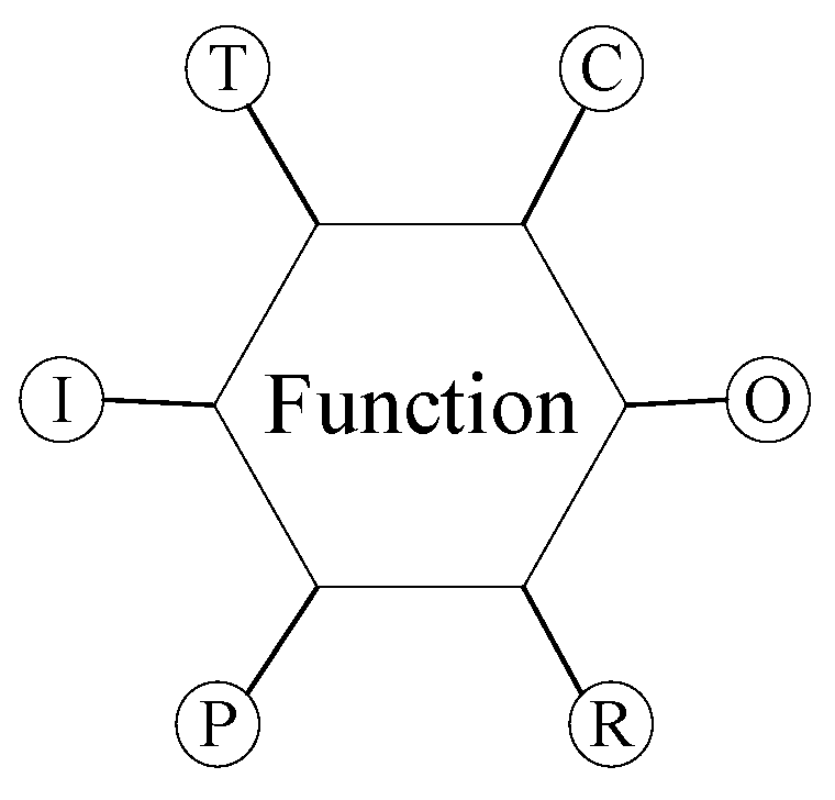
In FRAM, functional modules are described by six attributes—Input (I), Output (O), Preconditions (P), Resources (R), Time (T), and Control (C)—presented in a regular hexagonal shape, as shown in Figure 4.

The main steps of FRAM for assessing the fault risk in this study are as follows:

(1) Identify and describe the basic functions of the system. The relevant elements of the aircraft’s operation are linked in the form of a topological network, and the six attributes mentioned above are used to describe and characterize each functional module.

(2) Identify potential changes in each function. The changes in each functional module itself may lead to changes in other related functions. The operation of an aircraft involves factors such as people, aircraft, environment, and management. In order to quantify the mutual influences of these factors, first, an evaluation of the functional changes of each factor from different dimensions is necessary.

Set scores for functional modules in terms of time and accuracy to quantify the functional Output Variability (OV) of the modules. The performance of functional modules in terms of time can be divided into too early, on time, too late, and not occurring, and the performance in terms of accuracy can be divided into precise, acceptable, and imprecise. The calculation method for the OV is shown as follows:

$$OV=Q_T\times Q_P$$

(14)

where $Q_T$ represents the score of a temporal performance deviation for a system functional module, with the values 1 (on time), 2 (too early), 3 (too late), and 4 (non-occurrence); $Q_P$ represents the score of precision-related performance deviation, with values of 1 (precise), 2 (acceptable), and 3 (imprecise) as shown in

Table 5. Performance deviation scores.

Category	Performance Deviation	Score
Time	On Time	1
	Too Early	2
	Too Late	3
	Non-occurring	4
Accuracy	Precise	1
	Acceptable	2
	Imprecise	3

. A higher OV value indicates greater functional variability and a higher likelihood of functional resonance.

(3) Analyze oscillations between functional modules. After identifying potential variations in each function, the coupling resonance effects between functional modules are analyzed by linking the attributes of upstream and downstream modules.

(4) Determine the risk damping coefficient in risk evolution paths. The variability of functional modules and the connection methods between upstream and downstream determine the trend of risk transmission. In order to quantify the impact of the above, the risk damping coefficient is set into three categories: damping, no impact, and negative damping.

$${\alpha }_T({\alpha }_P)=\left\{\begin{array}{ll}1.2,& negative damping\\ 1,& no impact\\ 0.8,& damping\end{array}\right.$$

(15)

where ${\alpha }_T$ and ${\alpha }_P$ are the risk damping coefficients derived from temporal and precision-related deviations of upstream outputs, respectively.

The coupling effects of upstream and downstream functional modules are shown in

Table 6. Table of values for propagation factors under different coupling effects.

Category	Performance Deviation	I	R	P	T	C
Time	On Time	damping	damping	damping	damping	damping
	Too Early	no impact	damping	damping	negative damping	negative damping
	Too Late	negative damping	negative damping	negative damping	negative damping	negative damping
	Non-occurring	negative damping	negative damping	negative damping	negative damping	negative damping
Accuracy	Precise	damping	damping	damping	damping	damping
	Acceptable	no impact	no impact	no impact	no impact	no impact
	Imprecise	negative damping	negative damping	negative damping	negative damping	negative damping

.

By integrating functional variability and the corresponding failure modes, the risk damping coefficient can be calculated using the following formula:

$$W=OV\times {\alpha }_T\times {\alpha }_P$$

(16)

4. Model Implementation and Case Analysis

In this study, the flap/slat subsystem in the aircraft control system is taken as the research object, and the IRPN failure risk assessment framework is applied to evaluate failure risks. The data of the instance comes from the operational data of a certain aircraft model of a certain airline company due to the confidentiality of the aircraft operational data in the case and limitations in length, and only the key results of the calculations are presented.

(1) Static Analysis of Failure Probability

The flap/slat system of the aircraft control system consists of electronic controllers, actuators, sensors, and other components. The FMECA results, obtained through an investigation of failure modes, causes, and impacts, are shown in

Table 7. System failure mode analysis.

Component	Failure Mode	Failure Cause	Failure Impact
Control Valve (M1)	Valve Jamming (M11)	Component aging, contamination, external damage	Flap/slat movement instability, inaccurate position
	Seal Failure (M12)
Flap/Slat Controller (M2)	Circuit Short Circuit (M21)	Material aging, external damage, voltage fluctuation	Signal transmission failure, abnormal flap/slat operation
	Software Error (M22)	Programming error, component aging
Flap/Slat Actuation Mechanism (M3)	Drive Mechanism Failure (M31)	Wear, corrosion, mechanical damage	Causing incorrect flap/slat deployment time and position data
	Actuation System Failure (M32)	Wear, mechanical damage, material fatigue	Inconsistent left and right flap commands, unintended roll
Flap/Slat Sensor (M4)	Sensor Failure (M41)	Damage, calibration error, environmental impact	Affects the accuracy of flap/slat control
Flap/Slat Surface (M5)	Surface Damage (M51)	Material aging	Decreased aerodynamic performance of flaps/slats, unstable aircraft movement

.

This study obtained Service Difficulty Reports in China’s civil aviation from 2018 to 2023 and estimated the failure probabilities of various systems and their components by statistically analyzing relevant failure data. In addition, by hiring maintenance personnel from airlines and employees from third-party aviation maintenance agencies, a conditional probability distribution table for Bayesian network nodes was created by reviewing maintenance records. Considering the difficulty of data acquisition, this article mainly focuses on the operation and maintenance failures caused by operational errors of maintenance personnel, as well as the probability of failures caused by adverse conditions such as bird strikes and thunderstorms, when considering the influences of human and environmental factors.

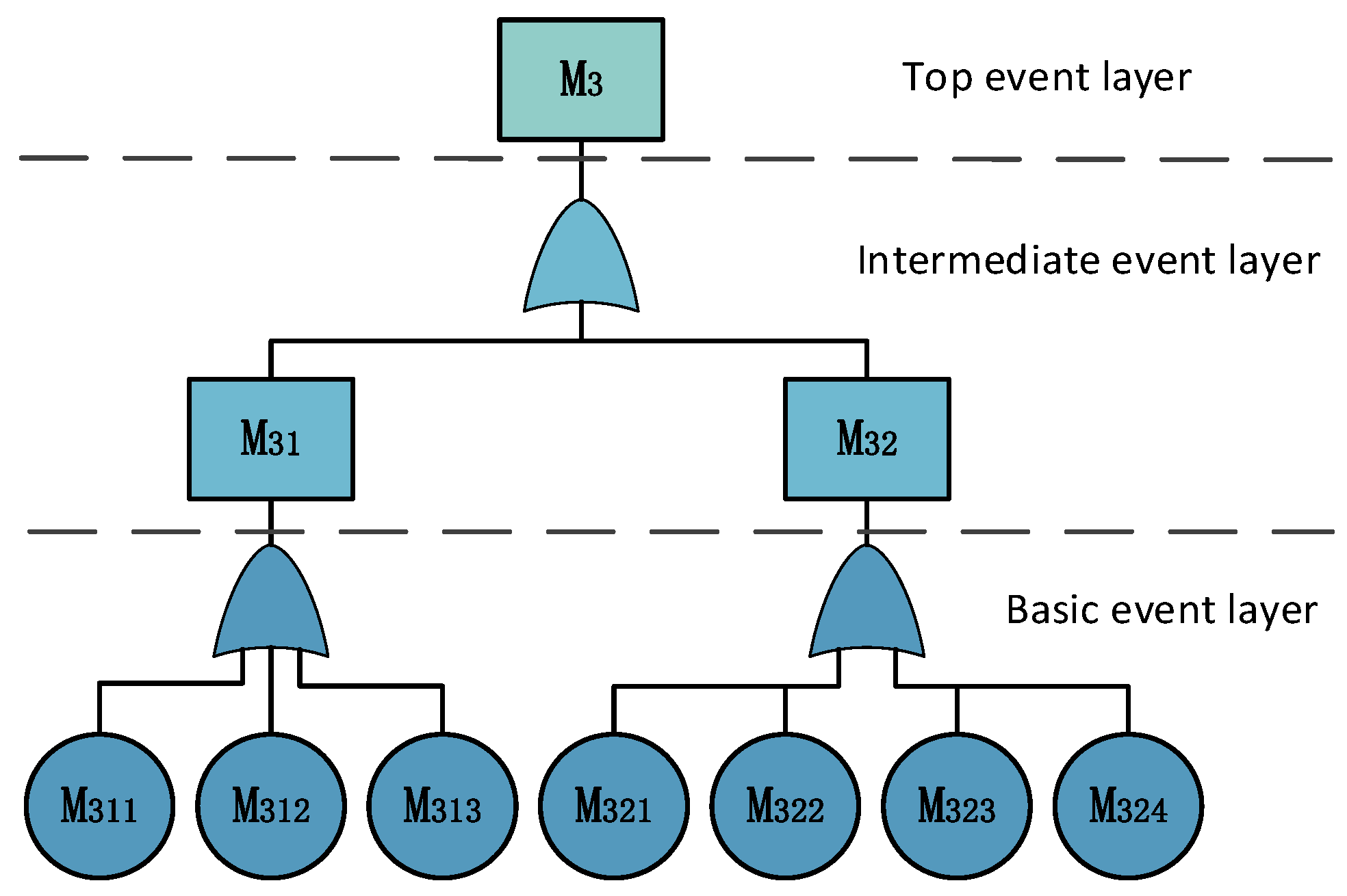
Using the flap/slat actuation mechanism (M3) event as an example, the top-level event is the failure of the flap/slat actuation mechanism (M3), with intermediate events including drive mechanism failure (M31) and actuation system failure (M32). Basic-level events include bearing failure, gearbox issues, and hydraulic system defects. Using the fault tree model (Figure 5) and Equations (2) and (3), the failure probability of M3 due to system faults is calculated as 1.87 × 10⁻⁴ (1.6 occurrences annually).

To account for the impacts of human factors (M6) and environmental factors (M7) on the failure probability of the flap/slat actuation mechanism (M3), parameter learning was conducted using Genie software by inputting prior probabilities for root nodes. The Bayesian network model of flap/slat faults is shown in Figure 6. In the Bayesian network model, node states are defined as “YES” (failure occurrence) and “NO” (no failure). Auxiliary nodes (X1–X4) were introduced to limit parent nodes to 3–4 per sub-node, simplifying the probability distribution tables and enhancing clarity for expert interpretation and questionnaire completion.

Under the combined effects of human and environmental factors, the failure probabilities of the flap/slat actuation mechanism (M3), drive mechanism failure (M31), and actuation system failure (M32) are updated to $M_3^{\prime },M_{31}^{\prime },M_{32}^{\prime }$, respectively. The results demonstrate that the static failure probability of the actuation mechanism increases from 1.87 × 10⁻⁴ (1.6 occurrences annually) to 3.34 × 10⁻⁴ (2.9 occurrences annually). This highlights the significant influences of human and environmental factors on system failure probabilities.

Based on the calculations using the FMECA-FTA-BN joint algorithm, the fault probability of the Flap/Slat actuation mechanism is detailed in

Table 8. Fault probability of the Flap/Slat actuation mechanism.

Symbol	Event Name	Probability
M3′	Flap/Slat Actuation Mechanism	3.34 × 10−4
M31′	Drive Mechanism Failure	2.51 × 10−4
M32′	Actuation System Failure	2.56 × 10−4
M61	Operational Failure	2.82 × 10−5
M71	Bird Strike	7.79 × 10−5
M72	Adverse Weather	4.55 × 10−6
M311	Gearbox Wear and Fracture	1.56 × 10−5
M312	Bearing Failure	7.99 × 10−5
M313	Electrical Connection Failure	3.04 × 10−5
M321	Hydraulic Pump Failure	1.02 × 10−6
M322	Hydraulic Line Blockage or Leakage	2.45 × 10−5
M323	Actuator Wear	3.48 × 10−5
M324	Control Valve Failure	1.20 × 10−6

.

(2) Fault Dynamic Prediction Model and Effectiveness Evaluation

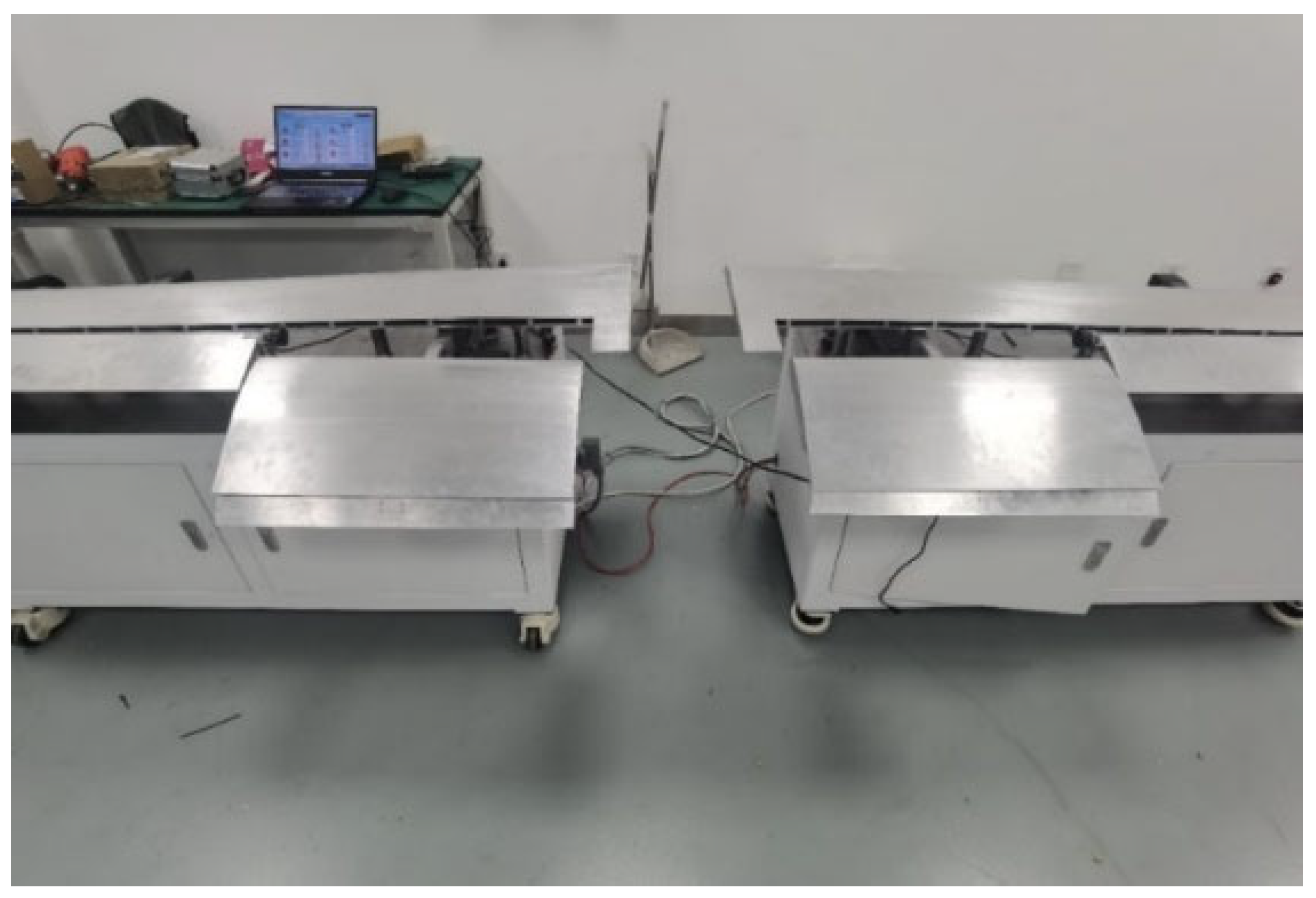
In order to accurately estimate the probability of failure, this paper uses the GRU neural network to dynamically predict the probability of jamming in the flap/slat motion mechanism (M3) system. The dataset is the key foundation for ensuring predictive performance. For this purpose, this study constructed a dataset that includes fault labels and multidimensional temporal features, covering a total of 22 features extracted from real QAR (Quick Access Recorder) data, including flap position parameters, flap control lever position parameters, and corresponding heights when flaps are closed and opened. Due to insufficient fault sample data in the database, in order to expand the fault samples and improve the generalization ability and prediction accuracy of the model, the aircraft flight control simulation experimental platform was used for fault simulation experiments in this study [44]. The experimental platform is constructed based on the structural design of the A320 aircraft model. The flap simulation system and aileron simulation system employ servo electric cylinders as the driving mechanism, which are fixed on a specially designed base through a matching design. Additionally, the experimental platform includes a pair of simulated wings connected to the base of the device via an optical axis and flange. The structural configuration of the experimental setup is illustrated in Figure 7.

In this study, time-series data is constructed to generate inputs for training the GRU neural network. Continuous time-series data segments are used as model inputs through time windows to capture the dynamic characteristics of the system. The input dimension of the GRU model is set to 22 (number of features), with 64 hidden layer neurons to ensure that the model has a sufficient learning capability. The model uses the Binary Cross-Entropy Loss function, with the Adam optimizer selected as the optimization algorithm. The learning rate (LR) is set to 0.001, batch size is 32, and the number of epochs is 20, aiming to minimize the loss function.

After evaluating accuracy (ACC), precision (PRE), recall (REC), and the balanced F score (F1), the trained GRU showed decent accuracy. In addition, this article also used LSTM and BP neural network algorithms to compare and verify the prediction results of GRU method in the field of flap/slat jamming faults, as shown in the

Table 9. Comparison table of prediction results.

Evaluation Criteria	BP	LSTM	GRU
ACC	93.15%	95.25%	95.13%
PRE	92.30%	92.80%	93.74%
REC	98.90%	99.80%	99.73%
F1	95.48%	96.12%	96.64%

.

In order to further compare the differences in computation time and memory usage among the three methods, this paper calculated the average training time, maximum training time, and average memory usage of each algorithm, as shown in the

Table 10. Comparison of computational performance.

Model	BP	LSTM	GRU
Avg. training time (s)	7.9	17.5	11.8
Max training time (s)	8.6	19.3	12.4
Avg. memory usage (kB)	19,825	30,092	23,275

.

In the comparative analysis of algorithm performance and efficiency, the BP, LSTM, and GRU models exhibit notable disparities in fault prediction tasks. GRU demonstrates the most superior comprehensive performance, achieving an F1 score of 96.64%—representing improvements of 0.52% and 1.16% over LSTM (96.12%) and BP (95.48%), respectively. In addition, GRU’s average training time and memory usage are reduced by 32.6% and 22.6%, respectively, compared to LSTM. While GRU is slower than the BP network (average 7.9 s), BP’s accuracy (93.15%) and recall (98.90%) are constrained by the limitations of shallow networks in addressing complex dynamic fault patterns.

In summary, GRU achieves a balance between prediction accuracy and computational efficiency through its simplified gating structure, making it more suitable for dynamic fault risk assessment scenarios in civil aviation systems that demand high real-time performance and reliability.

(3) Hybrid Prediction Model and Result Analysis

To better integrate the dynamic and static failure probability prediction results, a hybrid failure prediction model needs to be constructed. The possible fusion methods include the weighted average method, adjustment factor method, and threshold method. The weighted average method calculates the comprehensive risk probability by assigning fixed weights to static and dynamic predicted failure probabilities. But this method assumes that the static and dynamic failure probabilities vary linearly and cannot cope with the complex changes in system state. The adjustment factor method calculates the adjustment factor based on dynamic prediction results, which directly affect the static failure probability. However, this method has a strong dependence on adjustment factors and is easily affected by model errors. In this study, the threshold method was chosen, and a dynamic increment was introduced to replace the traditional fixed increment. This is because the threshold method can adjust the static fault probability reasonably based on the changes in dynamic fault probability, thereby enhancing the system’s ability to respond to real-time fault risks. Compared to the weighted averaging and adjustment factor methods, the threshold method is more flexible, does not rely on linear assumptions, and can better adapt to complex system state changes.

By calculating the difference between dynamic and static probabilities, the increment is dynamically adjusted, as shown in Equation (17):

$${\mathrm{O}}_{combined}=\left\{\begin{array}{cc}\hfill O_{static}\times f(O_{dynamic})\hfill & if O_{dynamic}>O_{static}\hfill \\ \hfill O_{static}\hfill & if O_{dynamic}<O_{static}\hfill \end{array}\right.$$

(17)

When the dynamic failure probabilities are high, increments increase significantly, whereas smaller gaps result in smaller adjustments. The formula is expressed as follows:

$$f(O_{dynamic})=\alpha \times \exp (\beta \times |O_{dymamic}-O_{static}|)$$

(18)

where α and β are constants adjusting the increment magnitude. $O_{dymamic}-O_{static}$ measures the deviation of the dynamic value from the static value. A larger deviation results in a higher exponentiated value under the influence of β. After exponential transformation and scaling by α, the output of the function $f(O_{dynamic})$ increases accordingly.

The parameter α determines the baseline scaling ratio of the increment. In order to simplify the calculation, maintain dimensional consistency, and facilitate subsequent tuning, α is set to one. β is used to control the sensitivity of the exponential term to the deviation between the dynamic value and the static value. If β is set to a smaller value, the mathematical model will fail to capture potential faults in a timely manner; conversely, an excessively large β may cause the model to overreact to normal fluctuations and trigger false alarms. By keeping α = 1.0 and other variables unchanged, β values were tested within a reasonable range. The prediction error (RMSE) was minimized when β was in the range of 4–6, and the model showed certain robustness. Therefore, β is set to five in this paper.

An example is provided to illustrate the calculation process of the model. For instance, when the gap between dynamic ($9.90\times {10}^{-3}$) and static ($3.34\times {10}^{-4}$) probabilities is $9.566\times {10}^{-3}$, the increment factor reaches 1.049, amplifying the static probability by 4.9%. The adjusted composite failure probability becomes $3.503\times {10}^{-4}$.

(4) Severity and Detectability Analysis

To quantitatively assess the levels of each evaluation characteristic parameter, the fuzzy comprehensive evaluation method was introduced, and 10 experts with diverse technical expertise were invited to conduct a comprehensive assessment based on the evaluation coefficient levels in

Table 11. Evaluation coefficient levels for various factors.

Influencing Factors	Level
	1	2	3	4	5
safety damage	Very Low	Low	Medium	High	Very high
equipment loss
maintenance cost

.

For the M3 jamming fault, fuzzy sets for safety damage, equipment loss, and maintenance cost were calculated using Equations (6)–(8). A fuzzy evaluation matrix was constructed and substituted into Equation (9) for computation.

$$N_3=\left[\begin{array}{ccccc}0.1& 0.1& 0.1& 0.3& 0.4\\ 0& 0.2& 0.2& 0.3& 0.3\\ 0& 0.2& 0.3& 0.2& 0.3\end{array}\right]$$

A pairwise comparison was made around the three evaluation criteria of “safety damage”, “equipment loss”, and “maintenance cost”, forming the following judgment matrix in

Table 12. Judgment matrix of the case.

	Safety Damage	Equipment Loss	Maintenance Cost
Safety Damage	1	3	5
Equipment Loss	1/3	1	4
Maintenance Cost	1/5	1/4	1

.

Using the Analytic Hierarchy Process (AHP) with Equations (10) and (11), the weight set for the parameters was determined as A = (0.62, 0.28, 0.10) and CR = 0.0825. After consistency validation, the judgment matrix meets the requirement. The composite fuzzy matrix was obtained by substituting the weights into Equation (12).

$$\begin{array}{c}{\mathrm{B}}_3=\mathrm{A}\times N_3\\ =\left[\begin{array}{ccc}0.62& 0.28& 0.10\end{array}\right]\left[\begin{array}{ccccc}0.1& 0.1& 0.1& 0.3& 0.4\\ 0& 0.2& 0.2& 0.3& 0.3\\ 0& 0.2& 0.3& 0.2& 0.3\end{array}\right]\\ =\left[\begin{array}{ccccc}0.062& 0.138& 0.148& 0.290& 0.362\end{array}\right]\end{array}$$

The results show that the severity of the actuation system fault is S₃ = 3.725.

A comprehensive evaluation of detection speed and diagnostic accuracy gave this fault mode an overall score of 3.8, indicating moderate detectability.

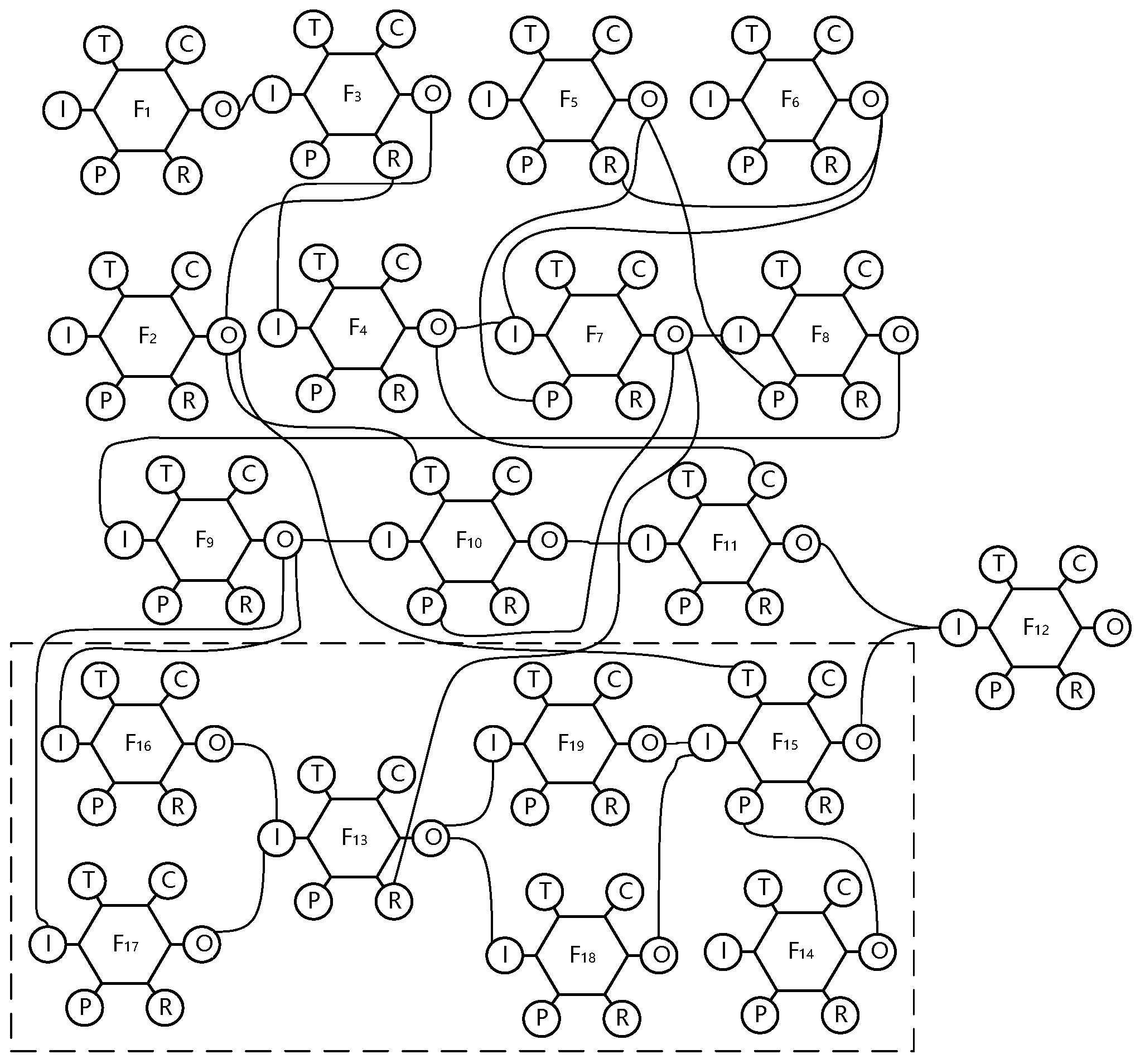
(5) Risk Damping Calculation

During the aircraft’s approach and landing phase, a jamming fault in the flap/slat actuation system may impact pilot operations and aircraft performance. To address this risk, system tasks and modules were decomposed in detail to analyze coupling effects and risk propagation pathways among actuation system modules, identifying 18 functional modules (F₁–F₁₉). The functional resonance network analysis diagram composed of various functional modules is shown in Figure 8.

Regarding the jamming fault of the flap actuation system, according to the QRH manual, pilots may implement three response measures. The functional modules of F₁–F₁₂ are propagated as response measures when landing using the backup flap system; F₁–F₉, F₁₂–F₁₃, F₁₅–F₁₆, and F₁₉ represent the response measures when the flap wing jamming is equal to zero and an alternate landing is implemented; F₁–F₉, F₁₇–F₁₈, and F₁₂–F₁₅ represent the measures taken when implementing alternate landing due to wing jamming greater than zero.

These modules include F₁, landing preparation; F₂, weather conditions; F₃, verification of the landing checklist; F₄, pilot execution of operations; F₅, fault identification; F₆, flap/slat position sensor; F₇, consultation of operational manual; F₈, selection of VFE (maximum flap extension speed); F₉, continuously check the PFD (primary flight display); F₁₀, adjust distance from the preceding aircraft; F₁₁, use of the backup flap system; F₁₂, execution of landing; F₁₃, calculation of fuel consumption and landing distance; F₁₄, air traffic service control; F₁₅, diversion landing; F₁₆, flap/slat jammed at zero position; F₁₇, flap/slat jammed above zero position; F₁₈, the selection of maximum speed minus 10 knots; and F₁₉, the selection of an appropriate flight speed. For example, as shown in

Table 13. Description of the functional parameters of functional module F₇.

Attributes	Description
I	Operation manual, aircraft status
O	Problem-solving solutions
C	Pilot’s consultation and operations
R	Operation manual
P	Detection of flap/slat jamming
T	Real time

, functional module F₇ (consultation of operation manual) is described using FRAM attributes. This method ensures that appropriate response measures are taken during flight operations to address flap/slat jamming faults, thereby reducing the impacts of such faults on flight safety performance.

Based on Table 4 and Table 6 and Figure 8, this article takes the coupling effect relationship between functional modules F₆ and F₅ as an example to illustrate. The pin “O” of functional module F₆ is connected to the pin “R” of F₅. When the time variation of F₆ is “on time”, “too early”, “too late”, or “non-occurring”, the risk damping coefficient transmitted from F₆ to F₅ are “damping”, “damping”, “negative damping”, and “negative damping”, respectively. That is, the value of damping coefficient of the time dimension can be set to 0.8, 0.8, 1.2, and 1.2, respectively. Similarly, from the perspective of accuracy, when the accuracy change of F₆ is “precise”, “acceptable”, and “imprecise”, the damping coefficients transmitted from F₆ to F₅ are “damping”, “no impact”, and “negative damping”, respectively, with corresponding coefficients of 0.8, 1, and 1.2. Therefore, based on the different damping coefficients of each functional module, the changes in risk transmission to the next functional module can be evaluated, and the final risk level can be calculated by superposition. In terms of the numerical evaluation of the functional variability of functional modules, this article draws on the method proposed by our research team in previous studies [45]. Due to the length of the paper, this calculation process will not be elaborated for now.

During the transition from Morphology 1 + F (flap/slat extension angle) to Morphology 0, the aircraft’s slats fail to fully retract to the clean configuration. Using the functional resonance analysis model, the risk damping coefficients for different operational scenarios were calculated. The functional variability of F₆ in terms of time and precision is $Q_T=2$ and $Q_P=3$, respectively. The risk damping coefficients for different scenarios are as follows:

Using backup flap system for landing, W = 1.015;

Flap/slat jammed at zero position (divert landing), W = 2.184;

Flap/slat jammed above zero position (divert landing), W = 3.694.

(6) Evaluation Results

Through the construction of the composite fault risk assessment framework, this study first conducted a preliminary static risk assessment, revealing a failure probability of $3.34\times {10}^{-4}$ for component M3. However, to enhance the system’s ability to respond to real-time fault risk variations during aircraft operation and improve assessment accuracy, a dynamic adjustment mechanism was introduced to nonlinearly correct the static probability. The resulting composite failure probability was calculated as $3.503\times {10}^{-4}$. This value indicates that dynamic environmental factors amplify the failure probability by approximately 4.9%, validating the enhanced risk sensitivity of the dynamic adjustment mechanism. According to the risk level classification in Table 1, this probability corresponds to Level 3 (Medium-High Risk), necessitating a further analysis of the system’s overall risk state by integrating additional parameters.

To comprehensively quantify the risk, all parameters were substituted into Equation (1):

Composite failure probability (O), $3.503\times {10}^{-4}$, derived from the coupling of static analysis and dynamic prediction.

Failure severity (S), 3.752, calculated using the Analytic Hierarchy Process (AHP) and fuzzy comprehensive evaluation method. The weights were allocated as safety damage (62%), equipment loss (28%), and maintenance cost (10%), with a consistency ratio (CR = 0.032) satisfying the validation requirements.

Detectability (D), 3.8, determined based on the detection speed and diagnostic accuracy level rules.

Risk damping (W), 3.694, quantified using the FRAM method, with the flap/slat jammed >0 position diversion scenario as a typical case to evaluate the resonance intensity between functional modules.

Substituting these parameters into Equation (1), the Improved Risk Priority Number (IRPN) was calculated as 158.00. According to the classification standard in Table 1, this value falls within the Controlled Risk range (90 ≤ IRPN < 160). The result deviates by only 1.25% from the severe risk threshold, emphasizing the need to suppress risk escalation through real-time monitoring of dynamic parameters. Although the current risk is controllable, the combined effects of high severity (S > 3.5) and moderate detectability (D < 4) highlight the necessity to continuously optimize fault diagnosis algorithms and enhance redundancy design, thereby reducing the IRPN value to a safer margin.

5. Conclusions

In view of the limitations of civil aircraft failure risk assessment research, an improved failure risk assessment composite model was proposed in this study, which was applied to the failure risk analysis of a flight control system. With the help of FMECA, FTA, Bayesian Network (BN), and GRU neural network technology, this paper significantly improves the accuracy of the fault probability calculation and accurately quantifies the evolution process of the risk after a failure occurrence by integrating static and dynamic failure probability calculation models and introducing risk damping coefficients.

Specifically, the conclusions of the study include the following aspects:

(1) This study proposes a hybrid model integrating static analysis and dynamic prediction, based on FMECA, FTA, Bayesian networks, and GRU neural networks. The model first quantifies the basic fault probabilities of system components through a static module (based on reliability data and statistical analysis), then uses GRU to dynamically capture temporal features, and updates these probabilities by coupling dynamic results with static values, forming a high-precision comprehensive prediction model. Experiments show that the model’s prediction accuracy (F1 score of 96.64%) significantly outperforms traditional RPN and single neural networks such as LSTM and BP, providing a new method with both theoretical and engineering value for fault risk assessments in complex systems.

(2) This study introduces risk damping coefficients. Based on the functional resonance analysis (FRAM), this study considers the risk damping coefficient as one of the risk factors for the fault risk assessment. This method can accurately analyze the coupling effects between different functional modules in the system and effectively predict the propagation path of risks. The experimental results indicate that the introduction of the risk damping coefficient not only increased the precision of the evaluation but also provided a strong basis for further optimizing fault response strategies.

(3) This study systematically verified the effectiveness and accuracy of the IRPN composite risk assessment framework in quantifying aircraft fault risks by constructing fault simulation experiments. Based on historical fault data, experimental results, simulation data, etc., dynamic deduction was conducted for the flap/slat jamming fault, and the comprehensive fault risk index calculated by the framework was cross-compared with actual records and traditional RPN assessment results. The results show that the IRPN framework can not only accurately identify high-risk faults but also effectively addresses the insufficiency of traditional methods in analyzing risk propagation in complex scenarios by introducing dynamic weight adjustment and multi-source data fusion mechanisms. The successful verification of this framework provides a reliable theoretical support and practical pathway for establishing real-time fault risk assessment systems in the aviation field.

(4) The fault risk composite assessment framework proposed in this study has good practicality and effectiveness for fault analysis and evaluation, and can be applied to other systems with dynamic fault risk assessment requirements and complete fault data records. However, due to the confidentiality constraints and low failure rate of aviation data, improvements can be made in increasing data collection and optimizing algorithm models in the future. In addition, the different fault characteristics exhibited by aircraft under different operating conditions, as well as the fault modes that are extremely related to operation, such as overloads, possible critical situations, etc., are worthy of in-depth research.