Guidance Laws for Multi-Agent Cooperative Interception from Multiple Angles Against Maneuvering Target

Abstract

To address the interception problem against maneuvering targets, this paper proposes a multi-agent cooperative guidance law based on a multi-directional interception formation. A three-dimensional agent–target engagement kinematics model is established, and a fixed-time observer is designed to estimate the target acceleration. By utilizing the agent-to-agent communication network, real-time exchange of motion state information among the agents is realized. Based on this, a control input along the line-of-sight (LOS) direction is designed to directly regulate the agent–target relative velocity, effectively driving the agent swarm to achieve time-to-go consensus within a fixed-time boundary. Furthermore, adaptive variable-power sliding mode control inputs are designed for both elevation and azimuth angles. By adjusting the power of the control inputs according to a preset sliding threshold, the proposed method achieves fast convergence in the early phase and smooth tracking in the latter phase under varying engagement conditions. This ensures that the elevation and azimuth angles of each agent–target pair converge to the desired values within a fixed-time boundary, forming a multi-directional interception formation and significantly improving the interception performance against maneuvering targets. Simulation results demonstrate that the proposed cooperative guidance law exhibits fast convergence, strong robustness, and high accuracy.

1. Introduction

With the continuous advancement of modern aerospace technology, high-speed maneuvering targets exhibit an increasingly enhanced capability to penetrate integrated air defense systems [1,2]. In this context, ensuring the effective interception of these targets, particularly when high-value targets are at risk [3,4], has emerged as a critical issue in contemporary air and space defense operations. In the interception of high-value aerial targets, traditional methods typically rely on single-agent engagement strategies [5]. However, such approaches impose stringent requirements on interceptor performance, resulting in elevated costs and an excessive dependence on the individual agent’s maneuverability, guidance accuracy, and warhead effectiveness [6]. These challenges lead to increased complexity in both design and manufacturing processes. To overcome these limitations, cooperative multi-agent interception has been proposed as a promising and cost-effective alternative [7]. By deploying multiple relatively low-cost interceptors, this strategy enables coordinated engagement of the target. Under the framework of a cooperative guidance law, the agents are driven to simultaneously approach the target from multiple directions. Subsequently, proximity fuzes initiate warhead detonation, forming a large-area fragmentation pattern that substantially enhances the probability and the overall interception effectiveness [8,9].

In recent years, cooperative multi-agent guidance technology has witnessed rapid development and has found broad applications in scenarios such as synchronized interception against high-value targets and coordinated interception of high-speed aerial threats [5,10]. Whether employed offensively as a “spear” or defensively as a “shield,” the core challenge in multi-agent cooperative operations lies in achieving consistency in the time-to-go among participating interceptors [11,12]. Generally, two methods are commonly adopted for time-to-go estimation. The first method computes the time-to-go based on the proportional navigation guidance (PNG) principle [13], while the second estimates it as the ratio of the agent–target relative distance to their relative velocity. Although the PNG-based approach considers multiple factors, it suffers from high computational complexity and often relies on an empirical constant, typically fixing the navigation ratio to three. Such assumptions may lead to poor adaptability and reduced accuracy under varying engagement conditions. In contrast, the second approach offers a more intuitive and computationally efficient solution by directly utilizing kinematic information. This simplicity makes it particularly attractive for cooperative guidance scenarios. Building upon the estimation of time-to-go, various cooperative guidance laws have been developed to steer agent formations towards coordinated interception. Literature [14] designs control inputs along both the tangential and normal directions of the agent trajectory. Although it achieves high control precision, it requires two independent control channels, which increases the computational and implementation burden on the agent’s onboard guidance and control system. The literature [15,16] generates acceleration commands along the line-of-sight (LOS) direction, directly regulating the agent–target relative velocity. By precisely shaping the closing speed, this approach facilitates fast and effective convergence of time-to-go among agents, making it particularly suitable for time-critical interception missions.

The design of cooperative guidance laws intrinsically relies on inter-agent communication networks, as each interceptor must continuously share its real-time motion states with the formation to compute appropriate control commands [17]. Currently, two main types of communication topologies are commonly adopted in agent formations: global communication network and distributed communication network. In a global communication network, all agents are able to directly exchange information with every other agent in the formation. Although this structure ensures complete information sharing and facilitates straightforward consensus algorithms, its practical implementation faces significant engineering challenges. These include the difficulty of establishing reliable long-range communication links among spatially dispersed agents and the adverse effects of communication delays [18]. Moreover, the failure of a single agent’s communication node could potentially compromise the entire cooperative interception system [19]. Unlike the global network, the distributed network allows each agent to communicate only with its local neighbors, thereby achieving coordinated guidance through decentralized information exchange. This approach fully exploits the advantages of swarm intelligence and is inherently resilient to communication failures [20,21]. Even if a subset of agents loses connectivity, the overall interception capability is preserved. Furthermore, the distributed framework mitigates communication delays associated with distant nodes and significantly reduces bandwidth requirements and system complexity. Instead of relying on predefined interception times, the formation dynamically adjusts the guidance commands based on the consensus of shared coordination variables, achieving time-to-go synchronization in a flexible and robust manner. Given its ability to accommodate uncertainties, adapt to dynamic scenarios, and efficiently utilize networked information, the distributed communication network has emerged as a focal point of recent research on cooperative agent guidance systems.

Early research on cooperative guidance primarily focused on static targets. Proportional navigation (PN)-based cooperative guidance laws were developed against stationary targets by synchronizing the interception time according to a pre-assigned schedule [22]. Subsequently, distributed cooperative guidance laws based on communication networks were proposed to improve system robustness. In particular, improved versions of the PN guidance law have been designed to mitigate the adverse effects of input delays and communication topology switching [23].

To further enhance synchronization performance, cooperative guidance strategies based on finite-time convergence were introduced [24], providing better control over the convergence time of the time-to-go. Building upon this, the literature [25] proposed a fixed-time consensus-based cooperative guidance law, which guarantees convergence within a fixed-time bound independent of the system’s initial conditions. While these guidance strategies offer satisfactory performance against static targets, they are less effective when dealing with maneuvering targets. To address this limitation, recent studies have extended cooperative guidance methods to dynamic scenarios. For example, the literature [26] analyzed the terminal capture region and introduced the concept of capture windows under heading angle constraints, allowing the computation of controllable margins for all feasible positions, thus improving interception performance against maneuvering targets.

It is worth noting that most existing cooperative guidance laws remain limited to two-dimensional (2D) scenarios [27], which are inconsistent with the actual three-dimensional (3D) interception environments encountered in practice. In recent years, some researchers have started extending cooperative guidance laws to 3D engagement scenarios. References [3,10] proposed a cooperative guidance strategy capable of achieving arrival-time consensus within finite time; however, their work has not been generalized to full 3D applications. Extending the guidance law from 2D to 3D is a crucial step toward practical engineering implementation. The literature [28] successfully applied cooperative guidance laws in 3D space by introducing a reference plane that decomposes the 3D dynamics into two orthogonal 2D components. Separate guidance laws were then designed for each component to achieve convergence of the agent formation’s motion states. Further, reference [29] addressed the 3D cooperative interception problem by establishing an agent–target LOS coordinate frame on top of the conventional ground-fixed coordinate system, enabling the formulation of a complete 3D relative motion dynamic model suitable for a cooperative guidance design.

Building upon the aforementioned research, this paper proposes a multi-agent, multi-directional cooperative interception guidance law for maneuvering targets. First, a fixed-time observer is designed to estimate the target’s acceleration. Based on this estimation, control inputs are developed along the three axes of the agent–target LOS coordinate frame, enabling the synchronization of the time-to-go and the coordination of azimuth and elevation angles. This approach not only ensures simultaneous interception by all agents but also forms a fan-shaped interception formation, significantly improving interception effectiveness. The main contributions of this work are summarized as follows:

1.

In the literature [25], a cooperative guidance law was proposed by combining time-to-go consensus control with finite-time convergence techniques. However, its convergence time depends on the initial state of the system. In contrast, the LOS-direction guidance law designed in this paper is based on a novel fixed-time control technique that guarantees convergence within a predefined time boundary, independent of the initial state, and is applicable to various communication topologies.

2.

The literature [30] addressed the control of elevation and azimuth angles by integrating sliding mode control with fixed-time control to ensure angle convergence within a fixed time boundary. In this paper, an adaptive sliding mode control scheme is proposed, which integrates fixed-time and finite-time control techniques. Specifically, the controller adaptively switches control commands based on the value of the sliding mode variable. In the first stage, a high-order sliding mode controller ensures rapid convergence to a predefined sliding threshold. Once the threshold is reached, the second stage reduces the order and incorporates finite-time control to achieve stable convergence to zero. Since the initial state of the second stage is determined by the predefined sliding threshold, the finite-time technique can achieve the effect of fixed-time convergence.

3.

Regarding the estimation of time-to-go, the key to achieving accurate time-consensus cooperative interception lies in ensuring that the error between the estimated and actual time-to-go converges to zero before the agents reach the target. In this paper, the proposed guidance law ensures that this estimation error asymptotically converges to zero under the Lyapunov stability framework, thereby guaranteeing highly accurate time-consensus cooperative interception.

The remainder of this paper is organized as follows: Section 2 describes the useful mathematical lemmas. The engagement geometry and problem formulation are presented in Section 3. The distributed guidance law against the maneuvering target is described in Section 4. Section 5 analyzes the relationship between the estimated time-to-go and the actual time-to-go, providing a rigorous validation of the estimation accuracy. The designed guidance law is simulated and verified in Section 6. Finally, the conclusions are presented in Section 7.

2. Preliminaries

2.1. Graph Theory

To achieve multi-agent, multi-angle coordinated interception of the same airborne target, an inter-agent communication network must be established. Through this network, each agent transmits its own motion information and compares it with neighboring agents, enabling dynamic adjustments to its motion state for optimal coordination. The communication network is shown in Figure 1. The communication network is shown in $G=(\nu ,\epsilon ,A)$, where $\nu$ represents the agent node set, $\epsilon \subseteq \nu \times \nu$ represents the connection relationships between the nodes, $A=\left[a_{ij}\right]\in R^{n\times n}$ represents the adjacency matrix, and $a_{ij}$ represents the elements in the adjacency matrix and represents the connection relationship between the agent nodes i and j. This paper defines the communication network as an undirected graph. Then, there exists $(i,j)\in \epsilon \iff (j,i)\in \epsilon$. This means that the agent nodes i and j can exchange parameter information to adjust their relative motion states. If $(i,j)\in \epsilon$ represents that the node j can receive information from node i. The agents adjacent to the node i are represented by $N_i=\{\left.j=\nu \right|(j,i)\in \epsilon \}$. If there exists $(j,i)\in \epsilon$, then define $a_{ij}=1$. Otherwise, $a_{ij}=0$. $G=(\nu ,\epsilon ,A)$ does not have self-loops; that is, there is no $a_{ii}=0$. The corresponding Laplacian matrix is defined as $L\left(A\right)=\left[l_{ij}\right]\in R^{n\times n}$, where $l_{ii}={\displaystyle \sum _{j=1}^n}{a}_{ij}$. When $i\ne j$, $l_{ij}=-a_{ij}$ [31,32].

Assumption 1.

When the inter-agent communication network topology is connected, meaning that there exists a path between any two agents, the eigenvalues of the Laplacian matrix L satisfy the following relationship: $0<{\lambda }_2\left(L\right)\le ,\dots ,{\lambda }_n\left(L\right)$, where ${\lambda }_2\left(L\right)$ is referred to as the algebraic connectivity of the topology graph.

2.2. Other Useful Lemmas

Lemma 1

([33]). Once there exists any m ∈ ^n×n that satisfies ${\mathbf{1}}^T\mathbf{m}=\mathbf{0}$, with ${\mathbf{m}}^T\mathcal{L}\mathbf{m}\ge {\lambda }_2{\mathbf{m}}^T\mathbf{m}$, where $\mathbf{1}$ is defined as a column vector with all elements equal to 1.

Lemma 2

([34]). Assuming $x_1,x_2,\dots ,x_n\ge 0$, and $0<p_1\le 1,1<p_2<+\infty$, then

$$\sum _{i=1}^n{x}_i^{p_1}\ge {\left(\sum _{i=1}^n{x}_i\right)}^{p_1}$$

(1)

$$\sum _{i=1}^n{x}_i^{p_2}\ge n^{1-p_2}{\left(\sum _{i=1}^n{x}_i\right)}^{p_2}$$

(2)

Lemma 3

([35]). Consider a $\left(m+1\right)th$ order, $m\in {\mathrm{N}}_{+}$; then the fixed-time observer can be constructed as

$$\left\{\begin{array}{c}{\dot{\widehat{x}}}_k=-{\dot{\widehat{x}}}_{k+1}-{\delta }_{k}si{g}^{{\chi }_k}\left({\tilde{x}}_k\right)-{\overline{\delta }}_{k}si{g}^{{\overline{\chi }}_k}\left({\tilde{x}}_k\right)\hfill \\ {\dot{\widehat{x}}}_{m+1}=-{\delta }_{m+1}si{g}^{{\chi }_{m+1}}\left({\tilde{x}}_1\right)-{\overline{\delta }}_{m+1}si{g}^{{\chi }_{m+1}}\left({\tilde{x}}_1\right)-\sigma sign\left({\tilde{x}}_1\right)\hfill \end{array}\right.$$

(3)

where ${\widehat{x}}_k$ is the estimated value of $x_k$, $k=1,2,\dots ,m+1$, ${\tilde{x}}_1={\widehat{x}}_1-{\tilde{x}}_1$, ${\delta }_k=k{\delta }_0-(k-1)$, ${\overline{\delta }}_k=k{\overline{\delta }}_0-(k-1)$, where ${\delta }_0\in (1-\mathrm{\Omega },1)$, ${\overline{\delta }}_0\in (11+\mathrm{\Omega })$, $\mathrm{\Omega }=0^{+}$, $\sigma >L$ is a positive constant; ${\delta }_k$ and ${\overline{\delta }}_k$ are positive constants; and $x^{m+1}+{\delta }_1{x}^m+\dots +{\delta }_{m}x+{\delta }_{m+1}$ and $x^{m+1}+{\overline{\delta }}_1{x}^m+\dots +{\overline{\delta }}_{m}x+{\overline{\delta }}_{m+1}$ are Hurwitz polynomials. The transition time from the initial moment to the stable tracking of ${\widehat{x}}_k$ by $x_k$ satisfies

$$T<{\displaystyle \frac{{\lambda }_{max}^a\left(P_1\right)}{\nu a}}+{\displaystyle \frac{1}{\overline{\nu }\overline{a}{\lambda }_{min}^{\overline{a}}\left(P_2\right)}}$$

(4)

where $a=1-{\chi }_0$, $\overline{a}={\overline{\chi }}_0-1$, $P_l$ is the solution of the Lyapunov equation $P_l{B}_l+B_l^T{P}_l=-Q_l$. $Q_l$ is a positive definite matrix. $l=1,2$, $\nu ={\displaystyle \frac{{\lambda }_{min}\left(Q_1\right)}{{\lambda }_{max}\left(P_1\right)}}$, $\overline{\nu }={\displaystyle \frac{{\lambda }_{min}\left(Q_2\right)}{{\lambda }_{max}\left(P_2\right)}}$, $B_l$ is

$$B_1=\left[\begin{array}{cc}-{\kappa }_1& \\ ⋮& I_m\\ -{\kappa }_m& \\ -{\kappa }_{m+1}-\eta & 0\end{array}\right],B_2=\left[\begin{array}{cc}-{\overline{\kappa }}_1& \\ ⋮& I_m\\ -{\overline{\kappa }}_m& \\ -{\overline{\kappa }}_{m+1}& 0\end{array}\right]$$

(5)

Lemma 4

([36]). Consider the following equation:

$$\dot{y}=-a{y}^{{\displaystyle \frac{m}{n}}}-b{y}^{{\displaystyle \frac{p}{q}}},y\left(0\right)=y_0$$

(6)

where $a>0,b>0$, m, n, p, q are both positive odd integers and satisfy $m>n,p<q$. There exists y, which converges to the origin within a fixed time, and the system’s stability time boundary is

$$T\le {\displaystyle \frac{1}{a}}{\displaystyle \frac{n}{m-n}}+{\displaystyle \frac{1}{b}}{\displaystyle \frac{q}{q-p}}$$

(7)

On the other hand, if $\theta \stackrel{\Delta }{=}\left[q\right(m-n)/n(q-p\left)\right]\le 1$, a more conservative stability time boundary can be obtained as

$$T\le {\displaystyle \frac{q}{q-p}}\left({\displaystyle \frac{1}{\sqrt{ab}}}{tan}^{-1}\sqrt{{\displaystyle \frac{a}{b}}}+{\displaystyle \frac{1}{a\theta }}\right)$$

(8)

Lemma 5

([28]). If there exists the equation

$$\dot{W}\left(x\right)+\vartheta W\left(x\right)+\varsigma W^{\rho }\left(x\right)\le 0$$

(9)

when $\vartheta ,\varsigma >0$ and $1>\rho >0$, $W\left(x\right)$ will converge to zero in finite time, as

$$T\le {\displaystyle \frac{1}{\vartheta (1-\rho )}}\mathrm{In}{\displaystyle \frac{\vartheta W^{1-\rho }\left(x_0\right)+\varsigma }{\varsigma }}$$

(10)

where $ln\left(x\right)$ represents the logarithmic function with the base e, $x_0$ representing the initial quantity.

3. Engagement Kinematic Model and Problem Statement

3.1. Engagement Kinematic Model

Figure 1 illustrates a schematic diagram of multiple agents forming a fan-shaped interception formation in space. The proximity fuze, in conjunction with a fragmentation warhead, creates a relatively large interception zone in front of the target. At high speeds. The fragments can form an effective interception area, thereby completing the interception mission. As shown in Figure 2, we consider an agent formation consisting of n agents intercepting a moving incoming target aircraft. Here, $OXYZ$ represents the ground coordinate system, and $O_{LOS}{X}_{LOS}{Y}_{LOS}{Z}_{LOS}$ represents the agent–target LOS coordinate system. It is assumed that the agent and the target can change their acceleration through actuators. $a_i$ and $v_i$ represent the acceleration vector and velocity vector of the agent, respectively. $a_{r,i}$, $a_{\vartheta ,i}$ and $a_{\phi ,i}$ represent the components of the agent’s acceleration vector along the three coordinate axes in the agent–target LOS coordinate system. $a_T$ and $v_T$ represent the the target’s acceleration vector and velocity vector. $v_i$ and $v_T$ respectively represent the velocity vectors of the interceptor and the target. The relative velocity between each interceptor and the target is derived from the interceptor’s velocity vector and the target’s velocity vector. $a_{Tr,i}$, $a_{T\vartheta ,i}$ and $a_{T\phi ,i}$ represent the components of the target’s acceleration vector along the three coordinate axes in the agent–target LOS coordinate system. The relative kinematic equations between the ith agent and the maneuvering target can be described by

$$\left\{\begin{array}{c}{\ddot{r}}_i=r_i{\dot{\vartheta }}_i^2+r_i{\dot{\phi }}_i^2{cos}^2{\vartheta }_i-a_{r,i}+a_{Tr,i}\hfill \\ {\ddot{\vartheta }}_i=-{\displaystyle \frac{2{\dot{r}}_i}{r_i}}{\dot{\vartheta }}_i-{\dot{\phi }}_i^{2}sin{\vartheta }_{i}cos{\vartheta }_i-{\displaystyle \frac{a_{\vartheta ,i}}{r_i}}+{\displaystyle \frac{a_{T\vartheta ,i}}{r_i}}\hfill \\ {\ddot{\phi }}_i=-{\displaystyle \frac{2{\dot{r}}_i}{r_i}}{\dot{\phi }}_i+2{\dot{\vartheta }}_i{\dot{\phi }}_{i}tan{\vartheta }_i+{\displaystyle \frac{a_{\phi ,i}}{r_{i}cos{\vartheta }_i}}-{\displaystyle \frac{a_{T\phi ,i}}{r_{i}cos{\vartheta }_i}}\hfill \end{array}\right.$$

(11)

where $r_i$, ${\vartheta }_i$, and ${\phi }_i$ are the relative distance, elevation angle, and azimuth angle between the $i-th$ agent and the target.

3.2. Problem Formulation

This study focuses on designing acceleration based on the LOS direction to ensure that all agents in the formation reach the target simultaneously, achieving coordinated time-consistent multi-agent arrival. As the agent formation approaches the target, the fuze activates near-field detection to determine the optimal detonation moment based on the target’s motion state.

To achieve the best interception effect, the acceleration design for the pitch and azimuth angles in the LOS coordinate system is utilized to guide the agent formation into a multi-directional coordinated interception formation before reaching the target. This expands the area of the intercept and improves the efficiency of the intercept.

Therefore, the key problems to be addressed in this study are as follows:

• Based on the dynamic agent target model, an acceleration adjustment strategy is designed along the LOS direction to regulate the agent flight state, ensuring that the time-to-go of all agents in the formation is synchronized before reaching the target.
• Address the error between the estimated and actual time-to-go to improve the accuracy of multi-agent coordinated arrival.
• Design control inputs to adjust elevation and azimuth angles, ensuring rapid convergence to the desired interception formation and enhancing target interception efficiency.

To address the above issues, we designed a fixed-time convergent control method to achieve arrival-time consistency. In this guidance law, the convergence time for arrival synchronization is determined solely by the control parameters. Unlike finite-time convergence methods, this approach does not depend on the initial state values of the system. Additionally, the designed acceleration input along the LOS direction ensures that the agent–target relative velocity converges to zero. We incorporate the estimated time-to-go calculation formula ${\widehat{t}}_{go,i}=-{\displaystyle \frac{r_i}{{\dot{r}}_i}}$, when $\ddot{r}=0$, ${\widehat{t}}_{go,i}=t_{go,i}$. At this point, the estimated time-to-go can be considered equal to the actual time-to-go, improving the accuracy of coordinated arrival. Additionally, to enable the agent formation to achieve a multi-directional coordinated interception pattern, acceleration inputs in both the azimuth and elevation dimensions are designed to drive their respective angles to converge to the desired values.

4. Design of Fixed-Time Cooperative Guidance Law Against the Maneuvering Target

In this section, we propose a three-dimensional multi-agent cooperative guidance law based on fixed-time control technology. First, an acceleration control input along the LOS direction is designed to ensure that all agents in the formation reach the target simultaneously. Beyond using LOS-directional control to achieve consistency in arrival-time within the formation of the agent, additional control inputs for elevation and azimuth angles are designed. These inputs guide the agents into a multidirectional interception formation as they approach the target, expanding the fragmentation warhead’s dispersion area and enhancing interception efficiency against maneuvering targets.

4.1. Guidance Law Design Based on the LOS Direction

This section designs the control input along the LOS direction, with the aim of driving all the agents in the formation to reach the target simultaneously and perform a synchronized interception mission. To drive the agents’ time-to-go to achieve consistent convergence, the estimated time-to-go deviations of each agent will be computed through the agent-to-agent communication network. Simply put, each agent compares its estimated time-to-go with that of its neighboring agents, using this as input to design the acceleration control along the LOS direction.

The time-to-go for the agent can be calculated using the following formula:

$${\widehat{t}}_{go,i}=-{\displaystyle \frac{r_i}{{\dot{r}}_i}}$$

(12)

where $r_i$ represents agent–target relative distance, and ${\dot{r}}_i$ is the agent–target relative velocity along the LOS direction, $i=1,2,\dots ,n$.

It is important to note that since the agent–target relative velocity along the LOS direction is not constant, the calculated value here does not represent the actual time-to-go in a strict sense. Instead, it should be regarded as the estimated time-to-go. The relationship between the estimated and actual time-to-go will be discussed and analyzed in detail in the next section. Define the time-to-go deviation, which is used to compare the time-to-go of neighboring agents based on the agent-to-agent communication topology. When the time-to-go deviation converges to zero, it can be considered that the agent and its neighboring agents have achieved synchronization of the arrival time. The time-to-go deviation is calculated using the following formula:

$${\epsilon }_{go,i}=\sum _{i=1}^n{a}_{ij}({\widehat{t}}_{go,i}-{\widehat{t}}_{go,j})$$

(13)

In the equation, $a_{ij}$ represents the elements of the adjacency matrix, $i=1,2,\dots ,n,$ $j=1,2,\dots ,n$. The agent acceleration input along the LOS direction is designed as follows:

$$a_{r,i}=r_i{\dot{\vartheta }}_i^2+r_i{\dot{\phi }}_i^2{cos}^2{\vartheta }_i+{\displaystyle \frac{{\dot{r}}_i^2}{r_i}}(k_1{\epsilon }_{go,i}^{{\displaystyle \frac{m_1}{n_1}}}+k_2{\epsilon }_{go,i}^{{\displaystyle \frac{p_1}{q_1}}})+{\widehat{a}}_{Tr,i}$$

(14)

where $k_1>0$, $k_2>0$, $m_1/n_1>1$, $p_1/q_1<1$. ${\widehat{a}}_{Tr,i}$ represents the estimated acceleration of the target along the LOS direction of the $i-th$ agent.

For the estimation of the target’s acceleration, we design the following fixed-time observer:

$$\left\{\begin{array}{c}{\ddot{\widehat{r}}}_i={\widehat{a}}_{Tr,i}+r_i{\dot{\vartheta }}_i^2+r_i{\dot{\phi }}_i^2{cos}^2{\vartheta }_i-a_{r,i}-{\delta }_{1,r}{\left({\dot{\widehat{r}}}_i-{\dot{r}}_i\right)}^{{\chi }_{1,r}}-{\overline{\delta }}_{1,r}{\left({\dot{\widehat{r}}}_i-{\dot{r}}_i\right)}^{{\overline{\chi }}_{1,r}}\hfill \\ {{\dot{\widehat{a}}}^{k-2}}_{Tr,i}={\widehat{a}}_{Tr,i}^{k-2}-{\delta }_{k,r}{\left({\dot{\widehat{r}}}_i-{\dot{r}}_i\right)}^{{\chi }_{k,r}}-{\overline{\delta }}_{k,r}{\left({\dot{\widehat{r}}}_i-{\dot{r}}_i\right)}^{{\overline{\chi }}_{k,r}},k=2,\dots ,m\hfill \\ {{\dot{\widehat{a}}}^{m-1}}_{Tr,i}=-{\delta }_{m+1,r}{\left({\dot{\widehat{r}}}_i-{\dot{r}}_i\right)}^{{\chi }_{m+1,r}}-{\overline{\delta }}_{k,r}{\left({\dot{\widehat{r}}}_i-{\dot{r}}_i\right)}^{{\overline{\chi }}_{k,r}}-{\sigma }_{r}sign({\dot{\widehat{r}}}_i-\dot{r})\hfill \end{array}\right.$$

(15)

In the equation, ${\dot{\widehat{r}}}_i$ is the observed value of ${\dot{r}}_i$, and ${\widehat{a}}_{Tr,i}^{k-2}$$k=3,\dots ,m+1$ is the observed value of the corresponding variable. ${\overline{\delta }}_{k,r}$, ${\delta }_{k,r}$, ${\chi }_{k,r}$, and ${\overline{\chi }}_{k,r}$ are determined according to Lemma 3.

Theorem 1.

Consider the $ith$ agent system in Equation (11) with the communication graph $G\left(A\right)$. The cooperative guidance law in Equation (14) guarantees that the fixed-time consensus objective of ${\epsilon }_{go,i}$ is achieved, where the settling time is bounded by

$$\begin{array}{c}{T}_1\le {\displaystyle \frac{q_1}{q_1-p_1}}\left({\displaystyle \frac{1}{\sqrt{k_1{k}_2{n}^{\frac{n_1-m_1}{2n_1}}{\lambda }_2{\left(L\right)}^{\frac{(m_1+n_1)(p_1+q_1)}{4n_1{q}_1}}}}}{tan}^{-1}\sqrt{{\displaystyle \frac{k_1{n}^{\frac{n_1-m_1}{2n_1}}{\lambda }_2{\left(L\right)}^{\frac{q_1(m_1+n_1)-n_1(p_1+q_1)}{2n_1{q}_1}}}{k_2}}}\right.\\ \left.+{\displaystyle \frac{1}{k_1{n}^{\frac{n_1-m_1}{2n_1}}{\lambda }_2{\left(L\right)}^{\frac{m_1+n_1}{2n_1}}\psi }}\right)\end{array}$$

(16)

where $\psi =q_1(m_1-n_1)/n_1(q_1-p_1)$.

Proof. 

According to Equations (11)–(13), it follows that

$${\dot{\widehat{t}}}_{go,i}={\displaystyle \frac{r_i^2{\dot{\vartheta }}_i^2}{{\dot{r}}_i^2}}+{\displaystyle \frac{r_i^2{\dot{\phi }}_i^2{cos}^2{\vartheta }_i}{{\dot{r}}_i^2}}-{\displaystyle \frac{r_i{a}_{r,i}}{{\dot{r}}_i^2}}+{\displaystyle \frac{r_i{a}_{Tr,i}}{{\dot{r}}_i^2}}-1$$

(17)

The following Lyapunov function is chosen:

$$V_1={\displaystyle \frac{1}{2}}{\widehat{t}}_{go}^{T}L{\widehat{t}}_{go}={\displaystyle \frac{1}{4}}\sum _{i=1}^n\sum _{j=1}^n{a}_{ij}{\left({\widehat{t}}_{go,j}-{\widehat{t}}_{go,i}\right)}^2$$

(18)

$${\displaystyle \frac{\partial V_1}{\partial {\widehat{t}}_{go,i}}}=-\sum _{j=1}^n{a}_{ij}({\widehat{t}}_{go,j}-{\widehat{t}}_{go,i})$$

(19)

According to Equation (17), we obtain

$$\begin{array}{c}\hfill \begin{array}{c}\begin{array}{cc}\hfill {\dot{V}}_1& =\sum _{i=1}^n{\displaystyle \frac{\partial V_1}{\partial {\widehat{t}}_{go,i}}}{\dot{\widehat{t}}}_{go,i}=\sum _{i=1}^n{\displaystyle \frac{\partial V_1}{\partial {\widehat{t}}_{go,i}}}\left({\displaystyle \frac{r_i^2{\dot{\vartheta }}_i^2}{{\dot{r}}_i^2}}+{\displaystyle \frac{r_i^2{\dot{\phi }}_i^2{cos}^2{\vartheta }_i}{{\dot{r}}_i^2}}-{\displaystyle \frac{r_i{a}_{r,i}}{{\dot{r}}_i^2}}+{\displaystyle \frac{r_i{a}_{Tr,i}}{{\dot{r}}_i^2}}-1\right)\hfill \\ & =-\sum _{i=1}^n{\epsilon }_{go,i}\left[k_1{\epsilon }_{go,i}^{{\displaystyle \frac{m_1}{n_1}}}+k_2{\epsilon }_{go,i}^{{\displaystyle \frac{p_1}{q_1}}}+{\displaystyle \frac{r_i}{{\dot{r}}_i^2}}(a_{Tr,i}-{\widehat{a}}_{Tr,i})-1\right]\hfill \\ & =-\sum _{i=1}^n\left[k_1{\epsilon }_{go,i}^{{\displaystyle \frac{m_1}{n_1}}+1}+k_2{\epsilon }_{go,i}^{{\displaystyle \frac{p_1}{q_1}}+1}+{\displaystyle \frac{r_i}{{\dot{r}}_i^2}}{\epsilon }_{go,i}(a_{Tr,i}-{\widehat{a}}_{Tr,i})-{\epsilon }_{go,i}\right]\hfill \\ & =-\sum _{i=1}^n{k}_1{\epsilon }_{go,i}^{{\displaystyle \frac{m_1}{n_1}}+1}-\sum _{i=1}^n{k}_2{\epsilon }_{go,i}^{{\displaystyle \frac{p_1}{q_1}}+1}-\sum _{i=1}^n{\displaystyle \frac{r_i}{{\dot{r}}_i^2}}{\epsilon }_{go,i}(a_{Tr,i}-{\widehat{a}}_{Tr,i})+\sum _{i=1}^n{\epsilon }_{go,i}\hfill \end{array}\end{array}\end{array}$$

(20)

Note that $e_i=a_{Tr,i}-{\widehat{a}}_{Tr,i}\to 0$ is always bounded in $T_{ob}<{\displaystyle \frac{{\lambda }_{max}^a\left(P_1\right)}{\nu a}}+{\displaystyle \frac{1}{\overline{\nu }\overline{a}{\lambda }_{min}^{\overline{a}}\left(P_2\right)}}$ due to the fixed-time convergence of Equation (15). Moreover, ${\displaystyle \sum _{i=1}^n}{\epsilon }_{go,i}=0$. The above equation can be further simplified as

$$\begin{array}{c}\hfill \begin{array}{c}\begin{array}{cc}\hfill {\dot{V}}_1& =-\sum _{i=1}^n{k}_1{\epsilon }_{go,i}^{{\displaystyle \frac{m_1}{n_1}}+1}-\sum _{i=1}^n{k}_2{\epsilon }_{go,i}^{{\displaystyle \frac{p_1}{q_1}}+1}\hfill \\ & =-\sum _{i=1}^n{k}_1({\epsilon }_{go,i}^2{)}^{{\displaystyle \frac{m_1+n_1}{2n_1}}}-\sum _{i=1}^n{k}_2({\epsilon }_{go,i}^2{)}^{{\displaystyle \frac{p_1+q_1}{2q_1}}}\hfill \end{array}\end{array}\end{array}$$

(21)

Based on $k_1>0$ and $k_2>0$, it can be further obtained that ${\dot{V}}_1=-{\displaystyle \sum _{i=1}^n}{k}_1({\epsilon }_{go,i}^2{)}^{{\displaystyle \frac{m_1+n_1}{2n_1}}}-{\displaystyle \sum _{i=1}^n}{k}_2({\epsilon }_{go,i}^2{)}^{{\displaystyle \frac{p_1+q_1}{2q_1}}}\le 0$. According to the properties of the Laplacian matrix, we can obtain ${\epsilon }_{go}=-L{t}_{go}$, where ${\widehat{t}}_{go}=\left[{\widehat{t}}_{go,1},{\widehat{t}}_{go,2},\dots ,{\widehat{t}}_{go,n}\right]$. According Lemma 2, the equation satisfies

$$\begin{array}{c}\hfill \begin{array}{c}\begin{array}{cc}\hfill {\dot{V}}_1& \le -k_1{n}^{{\displaystyle \frac{n_1-m_1}{2n_1}}}{\left(\sum _{i=1}^n{\epsilon }_{go,i}^2\right)}^{{\displaystyle \frac{m_1+n_1}{2n_1}}}-k_2{\left(\sum _{i=1}^n{\epsilon }_{go,i}^2\right)}^{{\displaystyle \frac{p_1+q_1}{2q_1}}}\hfill \\ \hfill & =-k_1{n}^{{\displaystyle \frac{n_1-m_1}{2n_1}}}{\left({\epsilon }_{go}^T{\epsilon }_{go}\right)}^{{\displaystyle \frac{m_1+n_1}{2n_1}}}-k_2{\left({\epsilon }_{go}^T{\epsilon }_{go}\right)}^{{\displaystyle \frac{p_1+q_1}{2q_1}}}\hfill \end{array}\end{array}\end{array}$$

(22)

For the Laplacian matrix, there exists a column vector with all elements equal to 1 that satisfies

$$\left\{\begin{array}{c}{\mathbf{1}}^{T}L\mathbf{1}={\left(L^{1/2}\mathbf{1}\right)}^T\left(L^{1/2}\mathbf{1}\right)=0\hfill \\ L^{1/2}\mathbf{1}=0\hfill \end{array}\right.$$

(23)

Then, there exists ${\mathbf{1}}^T{L}^{1/2}{\widehat{t}}_{go}=0$, and further $m=L^{1/2}{\widehat{t}}_{go}=0$ B, so the following inequality holds:

$${\epsilon }_{go}^T{\epsilon }_{go}\ge 2{\lambda }_2\left(L\right)V_1$$

(24)

Furthermore, we can obtain

$${\left(L^{1/2}{\widehat{t}}_{go}\right)}^{T}L\left(L^{1/2}{\widehat{t}}_{go}\right)={\widehat{t}}_{go}^T{L}^{1/2}L{L}^{1/2}{\widehat{t}}_{go}={\widehat{t}}_{go}^{T}LL{\widehat{t}}_{go}\ge {\lambda }_2{\widehat{t}}_{go}^{T}L{\widehat{t}}_{go}$$

(25)

Not only that, but also, based on ${\epsilon }_{go}=-L{\widehat{t}}_{go}$ and $V_1={\displaystyle \frac{1}{2}}{{\widehat{t}}_{go}}^{T}L{\widehat{t}}_{go}$, we can conclude that

$${{\epsilon }_{go}}^T{\epsilon }_{go}\ge 2{\lambda }_2\left(L\right)V_1$$

(26)

Combining with Equation (22), we can obtain

$$\begin{array}{c}\hfill \begin{array}{c}\begin{array}{cc}\hfill {\dot{V}}_1& \le -k_1{n}^{{\displaystyle \frac{n_1-m_1}{2n_1}}}{\left(2{\lambda }_2\left(L\right)V_1\right)}^{{\displaystyle \frac{m_1+n_1}{2n_1}}}-k_2{\left(2{\lambda }_2\left(L\right)V_1\right)}^{{\displaystyle \frac{p_1+q_1}{2q_1}}}\hfill \\ \hfill & \le -k_1{n}^{{\displaystyle \frac{n_1-m_1}{2n_1}}}{\lambda }_2{\left(L\right)}^{{\displaystyle \frac{m_1+n_1}{2n_1}}}{\left(2V_1\right)}^{{\displaystyle \frac{m_1+n_1}{2n_1}}}-k_2{\lambda }_2{\left(L\right)}^{{\displaystyle \frac{p_1+q_1}{2q_1}}}{\left(2V_1\right)}^{{\displaystyle \frac{p_1+q_1}{2q_1}}}\hfill \end{array}\end{array}\end{array}$$

(27)

Further, let $Y=\sqrt{2V_1}$, and differentiate it.

$$\dot{Y}={\displaystyle \frac{{\dot{V}}_1}{\sqrt{2V_1}}}$$

(28)

Thus,

$$\dot{Y}\le -k_1{n}^{{\displaystyle \frac{n_1-m_1}{2n_1}}}{\lambda }_2{\left(L\right)}^{{\displaystyle \frac{m_1+n_1}{2n}}}{Y}^{{\displaystyle \frac{m_1}{n_1}}}-k_2{\lambda }_2{\left(L\right)}^{{\displaystyle \frac{p_1+q_1}{2q_1}}}{Y}^{{\displaystyle \frac{p_1}{q_1}}}$$

(29)

When $\psi \stackrel{\Delta }{=}[q_1(m_1-n_1)/n_1(q_1-p_1)]\le 1$, the stability time boundary can be further updated as Equation (16). □

4.2. Design of Multi-Agent Interception Formation Control Method

Currently, the interception of aerial targets mainly relies on proximity fuzes and directional warheads. In practical interception scenarios, point-to-point interception is highly unlikely due to the existence of a certain miss distance. Therefore, under high closing speeds, as long as the warhead fragment dispersion zone forms an interception surface capable of capturing the target, successful interception can be achieved. The multi-directional interception formation proposed in this paper aims to create an interception net composed of multiple fragment dispersion zones formed by several agents surrounding the target. In the previous section, the cooperative guidance law for simultaneous multi-agent arrival on the target has been established. Next, to achieve the multi-directional cooperative interception formation of the agent swarm, acceleration inputs in the elevation and azimuth directions will be designed. The objective is to guide each agent within the swarm to arrange itself in the vicinity of the target according to the desired multi-directional interception formation through the designed control inputs.

4.2.1. Design of Elevation Angle Control Law

In the agent–target elevation angle control problem, an adaptive sliding mode control approach is designed to drive the deviation between each agent’s actual elevation angle and the predefined desired elevation angle to converge to zero within a fixed-time boundary. Define the deviation between the elevation angle and the desired elevation angle.

$${\epsilon }_{\vartheta ,i}={\vartheta }_i-{\vartheta }_{d,i}$$

(30)

Here, ${\vartheta }_{d,i}$ is a constant parameter representing the desired elevation angle of the $i-th$ agent, which is predetermined and embedded into the agent’s onboard computing unit prior to launch. When ${\epsilon }_{\vartheta ,i}\to 0$. This indicates that the elevation angle successfully converges to its desired value. Once both the elevation and azimuth angles complete their convergence within a fixed time, an efficient multi-directional interception formation of the agent swarm can be established. The specific design of the control input for the elevation angle is as follows:

$$\begin{array}{c}\hfill \begin{array}{c}\begin{array}{cc}\hfill a_{\vartheta ,i}& =-{\displaystyle \frac{r_i}{{k_{\vartheta }}_1{\tau }_{\vartheta }{\left|{\dot{\vartheta }}_i\right|}^{{\tau }_{\vartheta }-1}}}\left[-{k_{\vartheta }}_{1}si{g}^{{\gamma }_{\vartheta }}\left({s_{\vartheta ,}}_i\right)-{k_{\vartheta }}_{2}si{g}^{{\alpha }_{\vartheta }}\left({s_{\vartheta ,}}_i\right)-{\dot{\vartheta }}_i\right]\hfill \\ & -2{\dot{r}}_i{\dot{\vartheta }}_i-r_i{\dot{\phi }}_i^{2}sin{\vartheta }_{i}cos{\vartheta }_i+{\widehat{a}}_{T\vartheta ,i}\hfill \end{array}\end{array}\end{array}$$

(31)

where ${k_{\vartheta }}_1,{k_{\vartheta }}_2>0$, $1<{\tau }_{\vartheta }<2$, $0<{\alpha }_{\vartheta }<1$. ${\gamma }_{\vartheta }$ is designed as an adaptive factor, which adjusts the parameter according to the magnitude of the sliding mode value, ensuring a balance between the convergence speed and stability of the elevation angle. When ${s_{\vartheta ,}}_i>s_{\Delta }$, the design of ${\gamma }_{\vartheta }>1$. Here, $s_{\Delta }$ is the predefined sliding mode threshold. The adaptive factor is designed to vary with the sliding mode value to adjust the power order in the control law. A higher-order parameter is used for rapid convergence when the sliding mode value is large, while a lower-order parameter is adopted to enhance stability when the sliding mode value is small. The specific design is

$${\gamma }_{\vartheta }=\left\{\begin{array}{c}1,\left|{s_{\vartheta ,}}_i\right|<s_{\Delta }\hfill \\ {\beta }_{\vartheta },\left|s_{\vartheta i}\right|\ge s_{\Delta }\hfill \end{array}\right.,{\beta }_{\vartheta }>1$$

(32)

Note that the sliding mode is designed based on Equation (30), as described in the following:

$${s_{\vartheta ,}}_i={\epsilon }_{\vartheta ,i}+{k_{\vartheta }}_{1}si{g}^{{\tau }_{\vartheta }}\left({\dot{\epsilon }}_{\vartheta ,i}\right)$$

(33)

In the design of the control law, in order to alleviate the chattering phenomenon during the control process, the traditional $sign\left(x\right)$ function is replaced with the $si{g}^k\left(x\right)={\left|x\right|}^{k}sign\left(x\right)$ function as an improved alternative. This modification effectively reduces the chattering effect near the end of the control process. In addition, a piecewise control strategy is implemented based on a sliding mode threshold. When the sliding variable is small, a lower power term is used in the control output to reduce the control gain and limit the amplitude of control input variation.

Remark 1.

In Equation (31), ${\widehat{a}}_{T\vartheta ,i}$ represents the acceleration component of the target in the LOS coordinate system as observed by the fixed-time observer. The design of the fixed-time observer is referenced in the previous section for the LOS direction and will not be repeated here.

Theorem 2.

Consider the following sliding surface. Under the designed control input Equation (31), the deviation ${\epsilon }_{\vartheta ,i}$ of the elevation angle is guaranteed to converge to zero within the fixed-time boundary.

$$T_{\vartheta 2}\le {\displaystyle \frac{1}{{k_{\vartheta }}_1{2}^{\frac{{\beta }_{\vartheta }+1}{2}}}}·{\displaystyle \frac{2}{{\beta }_{\vartheta }-1}}+{\displaystyle \frac{1}{{k_{\vartheta }}_2{2}^{\frac{{\alpha }_{\vartheta }+1}{2}}}}·{\displaystyle \frac{1+{\beta }_{\vartheta }}{1-{\beta }_{\vartheta }}}+{\displaystyle \frac{1}{{k_{\vartheta }}_1(1-{\alpha }_{\vartheta })}}\mathrm{In}{\displaystyle \frac{2k_{\vartheta 1}{V}_2^{\frac{1-{\alpha }_{\vartheta }}{2}}{s}_{\Delta }+2{k_{\vartheta }}_2}{2{k_{\vartheta }}_2}}$$

(34)

Proof. 

The following Lyapunov function is chosen:

$$V_2={\displaystyle \frac{1}{2}}{s}_{\vartheta ,i}^2$$

(35)

The derivative of the Lyapunov function is computed as follows:

$${\dot{V}}_2={\dot{s}}_{\vartheta ,i}{s}_{\vartheta ,i}$$

(36)

The derivative of $s_{\vartheta ,i}$ in the expression is as follows:

$$\begin{array}{c}\hfill \begin{array}{c}\begin{array}{cc}\hfill {\dot{s}}_{\vartheta ,i}& ={\dot{\epsilon }}_{\vartheta ,i}+{k_{\vartheta }}_1{\tau }_{\vartheta }{\left|{\dot{\epsilon }}_{\vartheta ,i}\right|}^{{\tau }_{\vartheta }-1}{\ddot{\epsilon }}_{\vartheta ,i}={\dot{\vartheta }}_i+{k_{\vartheta }}_1{\tau }_{\vartheta }{\left|{\dot{\vartheta }}_i\right|}^{{\tau }_{\vartheta }-1}{\ddot{\vartheta }}_i\hfill \\ & ={\dot{\vartheta }}_i+{k_{\vartheta }}_1{\tau }_1{\left|{\dot{\vartheta }}_i\right|}^{{\tau }_{\vartheta }-1}\left[-{\displaystyle \frac{2{\dot{r}}_i}{r_i}}{\dot{\vartheta }}_i-{\dot{\phi }}_i^{2}sin{\vartheta }_{i}cos{\vartheta }_i-{\displaystyle \frac{a_{\vartheta ,i}}{r_i}}+{\displaystyle \frac{a_{T\vartheta }}{r_i}}\right]\hfill \end{array}\end{array}\end{array}$$

(37)

By combining Equations (31), (36), and (37),

$$\begin{array}{c}\hfill \begin{array}{c}\begin{array}{cc}\hfill {\dot{V}}_2& ={s_{\vartheta ,}}_i\left[-{k_{\vartheta }}_{1}si{g}^{{\gamma }_{\vartheta }}\left({s_{\vartheta ,}}_i\right)-{k_{\vartheta }}_{2}si{g}^{{\alpha }_{\vartheta }}\left({s_{\vartheta ,}}_i\right)\right]\hfill \\ & =-{k_{\vartheta }}_1{\left|{s_{\vartheta ,}}_i\right|}^{{\gamma }_{\vartheta }+1}-{k_{\vartheta }}_2{\left|{s_{\vartheta ,}}_i\right|}^{{\alpha }_{\vartheta }+1}\hfill \end{array}\end{array}\end{array}$$

(38)

Based on $k_{\vartheta 1}>0$ and $k_{\vartheta 2}>0$, it can be further obtained that ${\dot{V}}_2=-{k_{\vartheta }}_1{\left|{s_{\vartheta ,}}_i\right|}^{{\gamma }_{\vartheta }+1}-{k_{\vartheta }}_2{\left|{s_{\vartheta ,}}_i\right|}^{{\alpha }_{\vartheta }+1}\le 0$. In the following analysis, the predefined sliding mode threshold is used as a boundary to prove the fixed-time convergence in the first stage. When ${s_{\vartheta ,}}_i>s_{\Delta }$, ${\gamma }_{\vartheta }={\beta }_{\vartheta }>1$. Equation (38) can be further expressed as

$$\begin{array}{c}\hfill \begin{array}{c}\begin{array}{cc}\hfill {\dot{V}}_2& =-{k_{\vartheta }}_1{\left|{s_{\vartheta ,}}_i\right|}^{{\beta }_{\vartheta }+1}-{k_{\vartheta }}_2{\left|{s_{\vartheta ,}}_i\right|}^{{\alpha }_{\vartheta }+1}\hfill \\ & =-{k_{\vartheta }}_1{\left(2V_2\right)}^{{\displaystyle \frac{{\beta }_{\vartheta }+1}{2}}}-{k_{\vartheta }}_2{\left(2V_2\right)}^{{\displaystyle \frac{{\alpha }_{\vartheta }+1}{2}}}\hfill \\ & =-{k_{\vartheta }}_1{2}^{{\displaystyle \frac{{\beta }_{\vartheta }+1}{2}}}{V_2}^{{\displaystyle \frac{{\beta }_{\vartheta }+1}{2}}}-{k_{\vartheta }}_2{2}^{{\displaystyle \frac{{\alpha }_{\vartheta }+1}{2}}}{V_2}^{{\displaystyle \frac{{\alpha }_{\vartheta }+1}{2}}}\hfill \end{array}\end{array}\end{array}$$

(39)

According to Lemma 4, the first-stage convergence time of the elevation angle control is determined as follows:

$$T_{\vartheta 1}\le {\displaystyle \frac{1}{{k_{\vartheta }}_1{2}^{\frac{{\beta }_{\vartheta }+1}{2}}}}·{\displaystyle \frac{2}{{\beta }_{\vartheta }-1}}+{\displaystyle \frac{1}{{k_{\vartheta }}_2{2}^{\frac{{\alpha }_{\vartheta }+1}{2}}}}·{\displaystyle \frac{1+{\beta }_{\vartheta }}{1-{\beta }_{\vartheta }}}$$

(40)

When ${s_{\vartheta ,}}_i\le s_{\Delta }$, ${\gamma }_{\vartheta }=1$, Equation (38) can be further expressed as

$${\dot{V}}_2=-2{k_{\vartheta }}_1{V}_2-{k_{\vartheta }}_2{2}^{{\displaystyle \frac{{\alpha }_{\vartheta }+1}{2}}}{V_2}^{{\displaystyle \frac{{\alpha }_{\vartheta }+1}{2}}}$$

(41)

According to Lemma 5, the second-stage convergence time of the elevation angle control is determined as follows:

$$T_{\vartheta 2}\le {\displaystyle \frac{1}{{k_{\vartheta }}_1(1-{\alpha }_{\vartheta })}}\mathrm{In}{\displaystyle \frac{2k_{\vartheta 1}{V}_2^{\frac{1-{\alpha }_{\vartheta }}{2}}\left(s_{\Delta }\right)+2{k_{\vartheta }}_2}{2{k_{\vartheta }}_2}}$$

(42)

From the perspective of the overall control process, the first stage involves the convergence from the initial sliding mode value to the predefined sliding mode threshold. The convergence time boundary for this stage is determined as the fixed time $T_{\vartheta 1}$ through Lyapunov stability proof, where $T_{\vartheta 1}$ actually constrains ${s_{\vartheta ,}}_i\to 0$. However, the actual convergence process in the first stage is represented by ${s_{\vartheta ,}}_i\to s_{\Delta }$. Therefore, in practice, the true convergence time of the first stage is much smaller than $T_{\vartheta 1}$. The convergence in the second stage is represented by $T_{\vartheta 2}$. By referencing Lemma 5, the stability of the convergence process is proved using finite-time convergence. Compared with fixed-time convergence, finite-time convergence has a lower design complexity and fewer system requirements; however, its convergence time is less predictable and depends on the initial state. It is worth noting that, although the second stage is designed for finite-time convergence, its initial state is the predefined sliding mode threshold $s_{\Delta }$. Therefore, the time boundary $T_{\vartheta 2}$ for the second-stage control is also fixed. Considering the entire convergence process of the elevation angle, the fixed convergence time can be expressed as

$$T_2\le {\displaystyle \frac{1}{{k_{\vartheta }}_1{2}^{\frac{{\beta }_{\vartheta }+1}{2}}}}·{\displaystyle \frac{2}{{\beta }_{\vartheta }-1}}+{\displaystyle \frac{1}{{k_{\vartheta }}_2{2}^{\frac{{\alpha }_{\vartheta }+1}{2}}}}·{\displaystyle \frac{1+{\beta }_{\vartheta }}{1-{\beta }_{\vartheta }}}+{\displaystyle \frac{1}{{k_{\vartheta }}_1(1-{\alpha }_{\vartheta })}}\mathrm{In}{\displaystyle \frac{2k_{\vartheta 1}{V}_2^{\frac{1-{\alpha }_{\vartheta }}{2}}\left(s_{\Delta }\right)+2{k_{\vartheta }}_2}{2{k_{\vartheta }}_2}}$$

(43)

□

4.2.2. Design of Azimuth Angle Control Law

The previous section has completed the demonstration of the elevation angle control method. In this section, we will focus on the control input for the azimuth angle to complete the design of the multi-directional interception formation in three-dimensional space. Similar to the elevation angle, we define the azimuth angle deviation as

$${\epsilon }_{\phi ,i}={\phi }_i-{\phi }_{d,i}$$

(44)

The sliding mode surface design refers to Equation (33). It is expressed as $s_{\phi ,i}={\epsilon }_{\vartheta ,i}+k_{\phi 1}si{g}^{{\tau }_{\phi }}\left({\dot{\epsilon }}_{\phi ,i}\right)$.

Based on the above definitions, the agent–target azimuth control law is designed as

$$\begin{array}{c}\hfill \begin{array}{c}\begin{array}{cc}\hfill a_{\phi ,i}& ={\displaystyle \frac{r_{i}cos{\lambda }_{\vartheta ,i}}{{k_{\phi }}_1{\tau }_{\phi }{\left|{\dot{\lambda }}_{\phi ,i}\right|}^{{\tau }_{\phi }-1}}}\left[-{k_{\phi }}_{1}si{g}^{{\gamma }_{\phi }}\left({s_{\phi ,}}_i\right)-{k_{\phi }}_{2}si{g}^{{\alpha }_{\vartheta }}\left({s_{\phi ,}}_i\right)-{\dot{\lambda }}_{\phi ,i}\right]\hfill \\ & +2{\dot{r}}_i{\dot{\lambda }}_{\phi ,i}cos{\lambda }_{\vartheta ,i}-2r_i{\dot{\lambda }}_{\vartheta ,i}{\dot{\lambda }}_{\phi ,i}sin{\lambda }_{\vartheta ,i}+{\widehat{a}}_{T\phi ,i}\hfill \end{array}\end{array}\end{array}$$

(45)

where ${k_{\phi }}_1,{k_{\phi }}_2>0$, $1<{\tau }_{\phi }<2$, $0<{\alpha }_{\phi }<1$, $si{g}^k\left(x\right)={\left|x\right|}^{k}sign\left(x\right)$. ${\gamma }_{\phi }$ is an adaptive factor referring to Equation (32). The design of the fixed-time observer for ${\widehat{a}}_{T\phi ,i}$ can refer to Equation (15).

Theorem 3.

Consider the following sliding surface. Under the designed control input, Equation (45), the deviation of the azimuth angle is guaranteed to converge to zero within the fixed-time boundary, as follows:

$$T_3\le {\displaystyle \frac{1}{{k_{\phi }}_1{2}^{\frac{{\beta }_{\phi }+1}{2}}}}·{\displaystyle \frac{2}{{\beta }_{\phi }-1}}+{\displaystyle \frac{1}{{k_{\phi }}_2{2}^{\frac{{\alpha }_{\phi }+1}{2}}}}·{\displaystyle \frac{1+{\beta }_{\phi }}{1-{\beta }_{\phi }}}+{\displaystyle \frac{1}{{k_{\phi }}_1(1-{\alpha }_{\phi })}}\mathrm{In}{\displaystyle \frac{2k_{\phi 1}{V}_2^{\frac{1-{\alpha }_{\phi }}{2}}\left(s_{\Delta }\right)+2{k_{\phi }}_2}{2{k_{\phi }}_2}}$$

(46)

Proof. 

The following Lyapunov function is chosen:

$$V_3={\displaystyle \frac{1}{2}}{s}_{\phi ,i}^2$$

(47)

The derivative of the Lyapunov function is computed as follows:

$${\dot{V}}_3={\dot{s}}_{\phi ,i}{s}_{\phi ,i}$$

(48)

where

$${\dot{s}}_{\phi ,i}={\dot{\epsilon }}_{\phi ,i}+{k_{\phi }}_1{\tau }_{\phi }{\left|{\dot{\epsilon }}_{\phi ,i}\right|}^{{\tau }_{\phi }-1}{\ddot{\epsilon }}_{\phi ,i}={\dot{\vartheta }}_i+{k_{\phi }}_1{\tau }_{\phi }{\left|{\dot{\phi }}_i\right|}^{{\tau }_{\vartheta }-1}{\ddot{\phi }}_i$$

(49)

In the following analysis, the predefined sliding mode threshold is used as a boundary to prove the fixed-time convergence in the first stage.

When ${s_{\phi ,}}_i>s_{\Delta }$

$$\begin{array}{c}\hfill \begin{array}{c}\begin{array}{cc}\hfill {\dot{V}}_3& =-{k_{\phi }}_1{\left|{s_{\phi ,}}_i\right|}^{{\beta }_{\phi }+1}-{k_{\phi }}_2{\left|{s_{\phi ,}}_i\right|}^{{\alpha }_{\phi }+1}\hfill \\ & =-{k_{\phi }}_1{\left(2V_3\right)}^{{\displaystyle \frac{{\beta }_{\phi }+1}{2}}}-{k_{\phi }}_2{\left(2V_3\right)}^{{\displaystyle \frac{{\alpha }_{\phi }+1}{2}}}\hfill \\ & =-{k_{\phi }}_1{2}^{{\displaystyle \frac{{\beta }_{\phi }+1}{2}}}{V_3}^{{\displaystyle \frac{{\beta }_{\phi }+1}{2}}}-{k_{\phi }}_2{2}^{{\displaystyle \frac{{\alpha }_{\phi }+1}{2}}}{V_3}^{{\displaystyle \frac{{\alpha }_{\phi }+1}{2}}}\hfill \end{array}\end{array}\end{array}$$

(50)

According to Lemma 4, the first-stage convergence time is determined as follows:

$$T_{\phi 1}\le {\displaystyle \frac{1}{{k_{\phi }}_1{2}^{\frac{{\beta }_{\phi }+1}{2}}}}·{\displaystyle \frac{2}{{\beta }_{\phi }-1}}+{\displaystyle \frac{1}{{k_{\phi }}_2{2}^{\frac{{\alpha }_{\phi }+1}{2}}}}·{\displaystyle \frac{1+{\beta }_{\phi }}{1-{\beta }_{\phi }}}$$

(51)

When ${s_{\phi ,}}_i\le s_{\Delta }$, we can obtain

$${\dot{V}}_3=-2{k_{\phi }}_1{V}_3-{k_{\phi }}_2{2}^{{\displaystyle \frac{{\alpha }_{\phi }+1}{2}}}{V_3}^{{\displaystyle \frac{{\alpha }_{\phi }+1}{2}}}$$

(52)

According to Lemma 5, the second-stage convergence time $T_{\phi 2}$ is

$$T_{\phi 2}\le {\displaystyle \frac{1}{{k_{\phi }}_1(1-{\alpha }_{\phi })}}\mathrm{In}{\displaystyle \frac{2k_{\phi 1}{V}_3^{\frac{1-{\alpha }_{\phi }}{2}}\left(s_{\Delta }\right)+2{k_{\phi }}_2}{2{k_{\vartheta \phi }}_2}}$$

(53)

Considering the entire convergence process of the azimuth angle, the fixed convergence time can be expressed as

$$T_3\le {\displaystyle \frac{1}{{k_{\phi }}_1{2}^{\frac{{\beta }_{\phi }+1}{2}}}}·{\displaystyle \frac{2}{{\beta }_{\phi }-1}}+{\displaystyle \frac{1}{{k_{\phi }}_2{2}^{\frac{{\alpha }_{\phi }+1}{2}}}}·{\displaystyle \frac{1+{\beta }_{\phi }}{1-{\beta }_{\phi }}}+{\displaystyle \frac{1}{{k_{\phi }}_1(1-{\alpha }_{\phi })}}\mathrm{In}{\displaystyle \frac{2k_{\phi 1}{V}_2^{\frac{1-{\alpha }_{\phi }}{2}}\left(s_{\Delta }\right)+2{k_{\phi }}_2}{2{k_{\phi }}_2}}$$

(54)

□

5. Guidance Law Performance Analysis

In the previous sections, we have completed the proof of the multi-agent cooperative guidance law designed for the consistency of time-to-go. The results show that the proposed guidance law is capable of achieving synchronous interception of the target within a fixed-time boundary. However, regarding the calculation of time-to-go, when the agent–target relative velocity ${\dot{r}}_i$ is not constant, the computed result is strictly only an estimated time-to-go. The relationship between the estimated time-to-go and the actual time-to-go can be derived from Equation (11) as follows:

$${\ddot{r}}_i=r_i{\dot{\vartheta }}_i^2+r_i{\dot{\phi }}_i^2{cos}^2{\vartheta }_i-a_{r,i}+a_{Tr,i}$$

(55)

Substituting into Equation (14),

$${\ddot{r}}_i=-{\displaystyle \frac{{\dot{r}}_i^2}{r_i}}(k_1{\epsilon }_{go,i}^{{\displaystyle \frac{m_1}{n_1}}}+k_2{\epsilon }_{go,i}^{{\displaystyle \frac{p_1}{q_1}}})-{\widehat{a}}_{Tr,i}+a_{Tr,i}$$

(56)

According to the fixed-time observer in Equation (15), within the fixed-time boundary, $T_{ob}<{\displaystyle \frac{{\lambda }_{max}^a\left(P_1\right)}{\nu a}}+{\displaystyle \frac{1}{\overline{\nu }\overline{a}{\lambda }_{min}^{\overline{a}}\left(P_2\right)}}$, $e_i=a_{Tr,i}-{\widehat{a}}_{Tr,i}\to 0$. Equation (56) can be further rewritten as

$${\ddot{r}}_i=-{\displaystyle \frac{{\dot{r}}_i^2}{r_i}}(k_1{\epsilon }_{go,i}^{{\displaystyle \frac{m_1}{n_1}}}+k_2{\epsilon }_{go,i}^{{\displaystyle \frac{p_1}{q_1}}})$$

(57)

In this equation, the time-to-go deviation ${\epsilon }_{go,i}$ can be driven to converge to zero within the fixed-time boundary defined in Equation (16) under the control of Equation (14). When ${\epsilon }_{go,i}=0$, it is evident that ${\ddot{r}}_i=0$.

In summary, it can be concluded that beyond the fixed-time boundary, the agent–target relative velocity can be regarded as constant. Therefore, the estimated time-to-go obtained from Equation (12) can be considered equal to the actual time-to-go. This not only ensures the consistency of time-to-go among the agents but also guarantees the accuracy of their arrival at the target.

6. Example Scenario

In this section, the results of the simulation are reported to illustrate the effectiveness of the proposed guidance law. Consider a coordinated interception scenario involving a swarm of five agents engaging a maneuvering target. The objective is to achieve time-synchronized interception while maintaining a spatial fan-shaped formation using the control inputs designed in this study. The initial states of each agent are provided in

Table 1. Initial state information.

Agent	${\mathit{r}}_{\mathit{i}}$ (m)	${\dot{\mathit{r}}}_{\mathit{i}}$ (m)	${\mathit{\vartheta }}_{\mathit{i}}$ (°)	${\mathit{\phi }}_{\mathit{i}}$ (°)	${\dot{\mathit{\vartheta }}}_{\mathit{i}}$ (°/s)	${\dot{\mathit{\phi }}}_{\mathit{i}}$ (°/s)	${\mathit{\vartheta }}_{\mathit{d},\mathit{i}}$ (°)	${\mathit{\phi }}_{\mathit{d},\mathit{i}}$ (°)
1	11000	−300	−25	25	0.1	0.15	0	0
2	12,000	−290	25	15	0.3	0.25	60	60
3	13,000	−310	−11	11	0.24	0.24	30	30
4	10,000	−330	−15	−30	−0.22	−0.2	−60	−60
5	11,500	−360	12	15	−0.12	−0.1	−30	−30

. The final selection of the control parameters is shown in

Table 2. Simulation parameters.

Parameter	Value
$k_1$	0.3
$k_2$	0.3
$p_1$	0.7
$p_2$	1.4
${k_{\vartheta }}_1$	1
${k_{\vartheta }}_2$	0.5
${k_{\phi }}_1$	1
${k_{\phi }}_2$	0.5
${\alpha }_{\vartheta }$	0.5
${\alpha }_{\phi }$	0.5
${\tau }_{\vartheta }$	1.2
${\tau }_{\phi }$	1.4
$s_{\Delta }$	10

. We take agents in a network with an undirected graph, as shown in Figure 3, which indicates that Node 1 can exchange information bidirectionally with Nodes 2 and 3. In the simulation, this is primarily reflected in the ability of adjacent nodes to share time-to-go information. Based on this, each agent can compute the time-to-go deviation relative to its neighbors, which in turn supports the adjustment of its control input. The interactions between Node 5 and Node 3, as well as between Node 4 and Nodes 2 and 3, follow a similar mechanism.

Figure 4a illustrates the flight trajectories of the agents and the target in three-dimensional space. As observed in conjunction with Figure 4b, all five agents successfully reach the target position at $t=36.4$ s, achieving coordinated interception. Figure 4c shows the trajectory of the target in three-dimensional space, where the red dot indicates the starting position and the black cross indicates the final position. Figure 4d presents the target’s acceleration along the X, Y, and Z axes. The amplitude of the target’s maneuvering acceleration is approximately within the range of $\pm 20{\mathrm{m}/\mathrm{s}}^2$. Figure 5a presents the time-to-go for each agent. As shown in Figure 5b, at the beginning of the control process, due to differences in the motion states of each agent, a deviation exists between the computed estimated time-to-go and the actual time-to-go. The maximum deviation occurs for $Agent3$ at the initial moment. Driven by the control input designed for time consistency, the estimation error between the computed and actual time-to-go approaches zero at approximately $t=6.4$ s. Furthermore, in Figure 6a, it can be observed that the relative velocity of each agent with respect to the target stabilizes after $t=6.4$, indicating that the agents enter a uniform motion phase relative to the target. This observation is consistent with the theoretical analysis of the guidance law presented in Section 5. Figure 6a shows that the control inputs in the LOS direction remain within $\pm 150{\mathrm{m}/\mathrm{s}}^2$. From an engineering application perspective, this control input range aligns well with practical constraints.

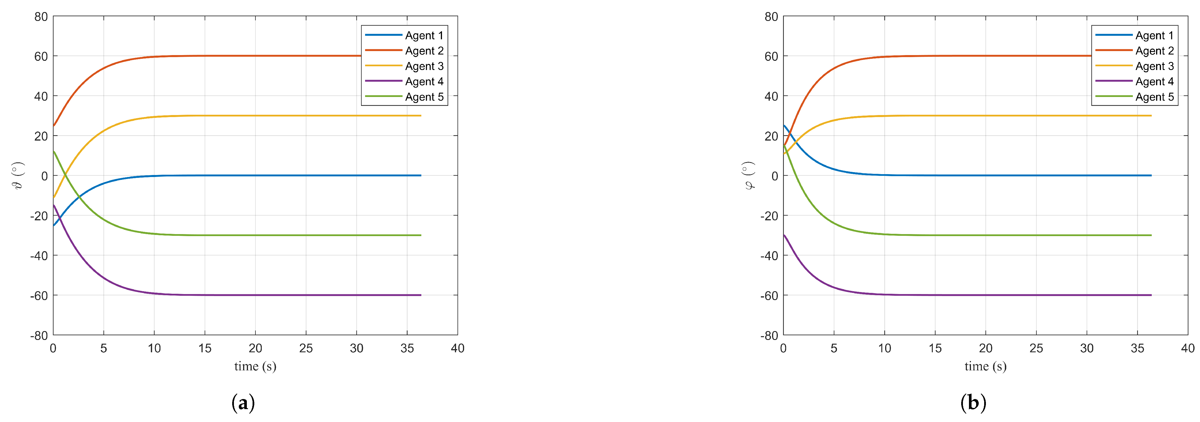
Figure 7a,b primarily demonstrate the effectiveness of the proposed control method for pitch and azimuth angles. When these angles are distributed according to the desired values, a fan-shaped interception formation is established in front of the target. This configuration increases the warhead fragment dispersion area, thereby enhancing interception effectiveness.

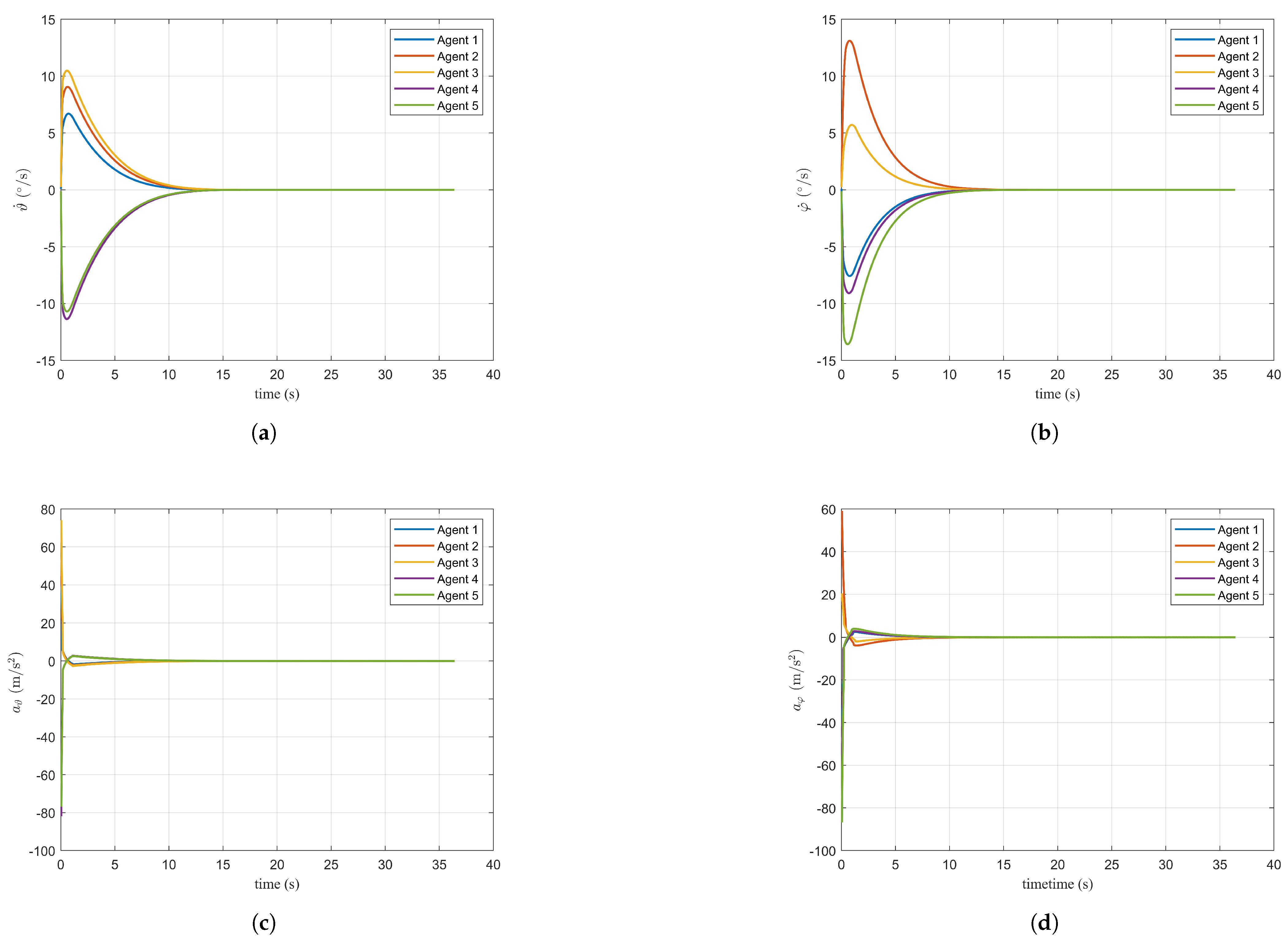
Figure 8a–d depict the control inputs for angular velocity and angular acceleration in both pitch and azimuth directions. As observed in the figures, the convergence times for these two angles are 12.8 s and 13.2 s, respectively. Similar to the LOS direction, the angular acceleration remains within a relatively small range of $\pm 100{\mathrm{m}/\mathrm{s}}^2$,which meets practical engineering application requirements.

Figure 9a,b correspond to the sliding mode surfaces designed for pitch and azimuth angle control. As shown in Table 2, the sliding mode threshold is set to $s_{\Delta }=10$ in the simulation. The local magnified view clearly shows a noticeable slope change at $s=10$, corresponding to the designed control input, which results in a change in the power term.

7. Conclusions

To address the interception requirements for maneuvering targets, this study proposes a multi-agent cooperative guidance law based on three-dimensional multi-directional interception. To achieve flight time consistency, a communication network is utilized to compare the time-to-go among neighboring agents, and the error is used as an input to design the control input in the agent–target LOS direction. Through an analysis of the consensus convergence process, the high-precision performance of the proposed guidance law in ensuring flight time consistency is further demonstrated. Furthermore, to overcome the spatial limitations of fragmentation dispersion in single-agent interception, a multi-agent, multi-directional interception formation is designed, enabling simultaneous detonation in front of the target to establish a fan-shaped interception zone. The control inputs for elevation and azimuth angles are designed using an adaptive variable power sliding mode control law, ensuring that these angles rapidly and stably converge to the desired values, thereby forming the designated interception formation. Simulation results validate that the proposed guidance law exhibits high precision, fast convergence rates, and strong robustness.

References

1. Dong, W.; Wang, C.; Wang, J.; Zuo, Z.; Shan, J. Fixed-time terminal angle-constrained cooperative guidance law against maneuvering target. IEEE Trans. Aerosp. Electron. Syst. 2021, 58, 1352–1366. [Google Scholar] [CrossRef]
2. Ziyan, C.; Jianglong, Y.; Xiwang, D.; Zhang, R. Three-dimensional cooperative guidance strategy and guidance law for intercepting highly maneuvering target. Chin. J. Aeronaut. 2021, 34, 485–495. [Google Scholar]
3. Ali, Z.A.; Han, Z.; Masood, R.J. Collective Motion and Self-Organization of a Swarm of UAVs: A Cluster-Based Architecture. Sensors 2021, 21, 3820. [Google Scholar] [CrossRef]
4. Niu, K.; Chen, X.; Yang, D.; Li, J.; Yu, J. A new sliding mode control algorithm of igc system for intercepting great maneuvering target based on edo. Sensors 2022, 22, 7618. [Google Scholar] [CrossRef]
5. Cevher, F.Y.; Leblebicioğlu, M.K. Cooperative Guidance Law for High-Speed and High-Maneuverability Air Targets. Aerospace 2023, 10, 155. [Google Scholar] [CrossRef]
6. Chen, W.; Hu, Y.; Gao, C.; An, R. Trajectory tracking guidance of interceptor via prescribed performance integral sliding mode with neural network disturbance observer. Def. Technol. 2024, 32, 412–429. [Google Scholar] [CrossRef]
7. Paul, N.; Ghose, D. Longitudinal-acceleration-based guidance law for maneuvering targets inspired by hawk’s attack strategy. J. Guid. Control. Dyn. 2023, 46, 1437–1447. [Google Scholar] [CrossRef]
8. Yang, T.; Zhang, X.; Wang, T.; Sun, W.; Cheng, C. A Warped-Fast-Fourier-Transform-Based Ranging Method for Proximity Fuze. IEEE Sens. J. 2024, 24, 8241–8249. [Google Scholar] [CrossRef]
9. Chakravarti, M.; Majumder, S.B.; Shivanand, G. End-game algorithm for guided weapon system against aerial evader. IEEE Trans. Aerosp. Electron. Syst. 2021, 58, 603–614. [Google Scholar] [CrossRef]
10. Markham, K.C. Solutions of Linearized Proportional Navigation Equation for Missile with First-Order Lagged Dynamics. J. Guid. Control. Dyn. 2024, 47, 589–596. [Google Scholar] [CrossRef]
11. Jeon, I.S.; Karpenko, M.; Lee, J.I. Connections between proportional navigation and terminal velocity maximization guidance. J. Guid. Control. Dyn. 2020, 43, 383–388. [Google Scholar] [CrossRef]
12. Tahk, M.J.; Jeong, E.T.; Lee, C.H.; Yoon, S.J. Attitude Hold Proportional Navigation Guidance for Interceptors with Off-Axis Seeker. J. Guid. Control. Dyn. 2024, 47, 1015–1025. [Google Scholar] [CrossRef]
13. Kim, J.H.; Park, S.S.; Park, K.K.; Ryoo, C.K. Quaternion based three-dimensional impact angle control guidance law. IEEE Trans. Aerosp. Electron. Syst. 2021, 57, 2311–2323. [Google Scholar] [CrossRef]
14. Li, H.; Liu, Y.; Li, K.; Liang, Y. Analytical Prescribed Performance Guidance with Field-of-View and Impact-Angle Constraints. J. Guid. Control. Dyn. 2024, 47, 728–741. [Google Scholar] [CrossRef]
15. Fossen, T.I. An adaptive line-of-sight (ALOS) guidance law for path following of aircraft and marine craft. IEEE Trans. Control Syst. Technol. 2023, 31, 2887–2894. [Google Scholar] [CrossRef]
16. Fossen, T.I.; Aguiar, A.P. A uniform semiglobal exponential stable adaptive line-of-sight (ALOS) guidance law for 3-D path following. Automatica 2024, 163, 111556. [Google Scholar] [CrossRef]
17. Du, Y.; Liu, B.; Moens, V.; Liu, Z.; Ren, Z.; Wang, J.; Chen, X.; Zhang, H. Learning correlated communication topology in multi-agent reinforcement learning. In Proceedings of the 20th International Conference on Autonomous Agents and MultiAgent Systems, Online, 3–7 May 2021; pp. 456–464. [Google Scholar]
18. Fei, B.; Bao, W.; Zhu, X.; Liu, D.; Men, T.; Xiao, Z. Autonomous cooperative search model for multi-UAV with limited communication network. IEEE Internet Things J. 2022, 9, 19346–19361. [Google Scholar] [CrossRef]
19. Deng, C.; Wen, C.; Huang, J.; Zhang, X.M.; Zou, Y. Distributed observer-based cooperative control approach for uncertain nonlinear MASs under event-triggered communication. IEEE Trans. Autom. Control 2021, 67, 2669–2676. [Google Scholar] [CrossRef]
20. Liu, L.; Wang, D.; Peng, Z.; Han, Q.L. Distributed path following of multiple under-actuated autonomous surface vehicles based on data-driven neural predictors via integral concurrent learning. IEEE Trans. Neural Netw. Learn. Syst. 2021, 32, 5334–5344. [Google Scholar] [CrossRef]
21. He, Z.; Fan, S.; Wang, J.; Wang, P. Distributed observer-based fixed-time cooperative guidance law against maneuvering target. Int. J. Robust Nonlinear Control 2024, 34, 27–53. [Google Scholar] [CrossRef]
22. Yu, H.; Dai, K.; Li, H.; Zou, Y.; Ma, X.; Ma, S.; Zhang, H. Distributed cooperative guidance law for multiple missiles with input delay and topology switching. J. Frankl. Inst. 2021, 358, 9061–9085. [Google Scholar] [CrossRef]
23. Nian, X.; Niu, F.; Yang, Z. Distributed Nash equilibrium seeking for multicluster game under switching communication topologies. IEEE Trans. Syst. Man Cybern. Syst. 2021, 52, 4105–4116. [Google Scholar] [CrossRef]
24. Wang, Z.; Fang, Y.; Fu, W.; Ma, W.; Wang, M. Prescribed-time cooperative guidance law against manoeuvring target with input saturation. Int. J. Control 2023, 96, 1177–1189. [Google Scholar] [CrossRef]
25. Wang, C.; Dong, W.; Wang, J.; Shan, J.; Xin, M. Guidance law design with fixed-time convergent error dynamics. J. Guid. Control. Dyn. 2021, 44, 1389–1398. [Google Scholar] [CrossRef]
26. Guo, D.; Ren, Z. Rapid Generation of Terminal Engagement Window for Interception of Hypersonic Targets. J. Astronaut. 2021, 42, 333. [Google Scholar]
27. Han, T.; Shin, H.S.; Hu, Q.; Tsourdos, A.; Xin, M. Differentiator-based incremental three-dimensional terminal angle guidance with enhanced robustness. IEEE Trans. Aerosp. Electron. Syst. 2022, 58, 4020–4032. [Google Scholar] [CrossRef]
28. Zhou, J.; Yang, J. Smooth Sliding Mode Control for Missile Interception with Finite-Time Convergence. J. Guid. Control Dyn. 2015, 38, 1–8. [Google Scholar] [CrossRef]
29. Li, G.; Zuo, Z. Robust leader–follower cooperative guidance under false-data injection attacks. IEEE Trans. Aerosp. Electron. Syst. 2023, 59, 4511–4524. [Google Scholar] [CrossRef]
30. Wang, X.; Lu, H.; Yang, Y.; Zuo, Z. Three-dimensional time-varying sliding mode guidance law against maneuvering targets with terminal angle constraint. Chin. J. Aeronaut. 2022, 35, 303–319. [Google Scholar] [CrossRef]
31. Zuo, Z. Nonsingular Fixed-Time Consensus Tracking for Second-Order Multi-Agent Networks; Pergamon Press, Inc.: Oxford, UK, 2015. [Google Scholar]
32. Zou, Y. Coordinated trajectory tracking of multiple vertical take-off and landing UAVs. Automatica 2019, 99, 33–40. [Google Scholar] [CrossRef]
33. Olfati-Saber, R.; Murray, R.M. Consensus problems in networks of agents with switching topology and time-delays. IEEE Trans. Autom. Control 2004, 49, 1520–1533. [Google Scholar] [CrossRef]
34. Zuo, Z.; Defoort, M.; Tian, B.; Ding, Z. Distributed Consensus Observer for Multi-Agent Systems with High-Order Integrator Dynamics. IEEE Trans. Autom. Control 2019, 65, 1771–1778. [Google Scholar] [CrossRef]
35. Basin, M.; Shtessel, Y.; Aldukali, F. Continuous finite- and fixed-time high-order regulators. J. Frankl. Inst. 2016, 353, 5001–5012. [Google Scholar] [CrossRef]
36. Zuo, Z.; Tie, L. Distributed robust finite-time nonlinear consensus protocols for multi-agent systems. Int. J. Syst. Sci. 2016, 47, 1366–1375. [Google Scholar] [CrossRef]
Figure 1. Diagram of multi-agent interception.
Aerospace 12 00531 g001
Figure 2. Cooperative guidance geometry.
Aerospace 12 00531 g002
Figure 3. Communication network with an undirected graph.
Aerospace 12 00531 g003
Figure 4. Simulation results under the guidance law: (a) trajectories in (X,Y,Z) space, (b) agent–target relative distance, (c) target motion trajectory, and (d) target acceleration.
Aerospace 12 00531 g004
Figure 5. Simulation results under the guidance law: (a) time-to-go and (b) error of time-to-go.
Aerospace 12 00531 g005
Figure 6. Simulation results under the guidance law: (a) agent–target relative velocity and (b) agent–target LOS acceleration input.
Aerospace 12 00531 g006
Figure 7. Simulation results under the guidance law: (a) elevation angle and (b) azimuth angle.
Aerospace 12 00531 g007
Figure 8. Simulation results under the guidance law: (a) elevation angular velocity, (b) azimuth angular velocity, (c) elevation angular acceleration input, and (d) azimuth angular acceleration input.
Aerospace 12 00531 g008
Figure 9. Simulation results under the guidance law: (a) elevation sliding mode value and (b) azimuth sliding mode value.
Aerospace 12 00531 g009