Analysis of Congestion-Propagation Time-Lag Characteristics in Air Route Networks Based on Multi-Channel Attention DSNG-BiLSTM

Abstract

As air transportation demand continues to rise, congestion in air route networks has seriously compromised the safe and efficient operation of air traffic. Few studies have examined the spatiotemporal characteristics of congestion propagation under different time lag conditions. To address this gap, this study proposes a cross-segment congestion-propagation causal time-lag analysis framework. First, to account for the interdependency across segments in air route networks, we construct a point–line congestion state assessment model and introduce the FCM-WBO algorithm for precise congestion state identification. Next, the Multi-Channel Attention DSNG-BiLSTM model is designed to estimate the causal weights of congestion propagation between segments. Finally, based on these causal weights, two indicators—CPP and CPF—are derived to analyze the spatiotemporal characteristics of congestion propagation under various time lag levels. The results indicate that our method achieves over 90% accuracy in estimating causal weights. Moreover, the propagation features differ significantly in their spatiotemporal distributions under different time lags. Spatially, congestion sources tend to spread as time lag increases. We also identify segments that are likely to become overloaded, which serve as the primary receivers of congestion. Temporally, analysis of time-lag features reveals that because of higher traffic flow during peak periods, congestion propagates 36.92% more slowly than during the early-morning hours. By analyzing congestion propagation at multiple time lags, controllers can identify potential congestion sources in advance. They can then implement targeted interventions during critical periods, thereby alleviating congestion in real time and improving route-network efficiency and safety.

1. Introduction

Air transport is widely regarded as the most efficient mode for long-distance passenger and cargo transportation, playing a critical role in promoting economic development and enhancing global connectivity. It has become a key component of modern transportation systems [1]. In recent years, driven by steadily rising demand, the number of global flights has increased markedly. According to the “2024 Global Civil Aviation Flight Operations Report”, there were approximately 32.85 million departures in 2023, and this number rose to 34.76 million in 2024, representing a 5.88% increase. However, transport and economic geography has demonstrated that aviation activities exhibit significant spatial–temporal concentration, with pronounced agglomeration effects observed in busy airspaces such as hub airports [2]. Yet the rigid constraints imposed by airspace capacity and air traffic controller workload mean that highly concentrated flight operations can lead to a substantial decline in the operational efficiency of the air transport system [3]. Indeed, on-time performance dropped from 75.57% in 2019 to 73.69% in 2024. This ongoing reduction in on-time performance has exacerbated the problem of flight delays, which seriously undermines both the safety and efficiency of the air transport system [4]. Flight delays represent a major challenge to the sustainable development of civil aviation. To analyze the distribution and causes of flight delays, it is necessary to investigate whether congestion occurs during air traffic control operations and to understand its distribution patterns [5].

Congestion can be defined as the phenomenon that occurs when input demand exceeds a facility’s output capacity [6]. In an air transport system, this manifests as flow bottlenecks on air routes or within airspace when traffic demand cannot be accommodated in a given time unit. Depending on the configuration of the airspace, congestion results in different levels of operational capacity degradation, with typical indicators such as reduced aircraft speed and increased aircraft density. Building on this theoretical framework, current approaches primarily identify traffic flow bottlenecks by analyzing traffic state variables [7] or their derived metrics to quantify the impact of aircraft accumulation on airspace operational efficiency. These variable values are subsequently discretized into a fixed number of levels for classification purposes [8]; for example, traffic density exceeding a specified threshold is labeled as congested. However, congestion in the airspace inevitably interacts with adjacent segments rather than remaining localized. Once congestion arises at a given node, it propagates outward along aircraft movement paths. As the congested region expands, fluctuations in traffic flow and efficiency losses trigger a chain reaction, ultimately leading to wide-spread congestion across the network.

Currently, congestion issues within air route networks are especially pronounced in regions such as Europe, the United States, and China [9]. As the critical linkage between airports and en-route airspace, air route networks are fundamental to ensuring the safe and efficient operation of aircraft; their performance directly affects the organization and throughput of traffic flows. Moreover, once congestion emerges on an upstream segment within the air route network, it readily propagates throughout the network, triggering downstream segment congestion and cascading delay effects that ultimately degrade overall flight efficiency across a broad area [10]. Therefore, to enhance controllers’ situational awareness and mitigate flight delays, two key scientific challenges must be addressed: accurately detecting congestion within the air route network and elucidating the mechanisms and characteristics by which congestion spreads throughout that network. Resolving these challenges is vital for improving the overall efficiency of air traffic operations and is a necessary step toward achieving the Civil Aviation Administration of China’s (CAAC) goal, as outlined in the “Smart Aviation Development Roadmap”, of refining airspace management and reducing congestion in busy regions.

However, most existing congestion assessment studies focus on broad airspace environments such as terminal areas, neglecting the structural interactions that occur across segments within the air route network. Even aircraft on different segments may exert a mutual influence on each other due to variations in speed, route selection, and other factors. Overlooking these cross-segment dynamic interactions can result in the omission of latent congestion ’seed’ locations, thereby facilitating rapid congestion propagation. Moreover, prior research has largely concentrated on analyzing the mechanisms of flight-delay propagation, lacking a systematic modeling framework for characterizing congestion diffusion across the air route network, particularly one based on deep causal learning methods. Off-the-shelf deep causal inference models from other domains cannot readily accommodate the multi-segment coupling and the intricate propagation pathways inherent in air route networks. Consequently, it is necessary to develop a deep causal inference model tailored to this scenario to investigate the mechanisms and characteristics by which congestion spreads throughout the air route network.

To address these gaps, we propose the following innovative approaches. First, we develop a waypoint–segment congestion assessment model that quantifies cross-segment interactions by incorporating the congestion states at individual waypoints, thereby providing a systematic evaluation of each segment’s congestion level. Second, we introduce a Multi-Channel Attention Decoupling Causal Architecture-Based Sparse Nonlinear Granger BiLSTM (Multi-Channel Attention DSNG-BiLSTM) model. Grounded in nonlinear Granger causality theory, this model employs sparse regularization to generate a sparse weight matrix—mitigating overfitting—and utilizes a decoupling causal architecture to disentangle the relationships between each output sequence and its corresponding input sequences. Additionally, a self-attention mechanism is incorporated to capture spatiotemporal dependencies across segments, enabling the estimation of causal propagation weights for congestion within the air route network. Finally, we demonstrate the superiority of our methods through comparisons with conventional approaches and summarize the spatiotemporal propagation characteristics of congestion across different time-delay levels. The primary contributions of this paper are as follows:

(1)

For the air route network scenario, a point–line congestion assessment model was designed that combines waypoints and segments to comprehensively account for cross-segment congestion coupling effects. The Fuzzy C-Means Beluga Whale Optimization (FCM-WBO) algorithm was proposed to effectively identify different congestion states.

(2)

The Multi-Channel Attention DSNG-BiLSTM model was introduced and trained using an improved Gradient Iterative Shrinkage Thresholding Algorithm (GISTA) algorithm. Compared to traditional models such as Multilayer Perceptron (MLP), Recurrent Neural Network (RNN), and long short-term memory (LSTM), this model achieved up to a 16.82% increase in the R² metric and was the only one to exceed 90% accuracy in estimating causal weights for congestion propagation. Based on these causal weights, two additional metrics—Congestion Propagation Potential (CPP) and Congestion Propagation Flux (CPF)—were proposed to form a more accurate understanding of the intrinsic causal relationships governing congestion propagation within the air route network.

(3)

Using the air route network in China’s south-central region as a case study, the spatiotemporal propagation patterns of network congestion at different time-delay levels were examined. Spatially, the characteristics of source segments and potential burdened segments were identified, revealing that 10% of segments accounted for 40.42% of the total congestion propagation. Temporally, differences in propagation characteristics due to varying traffic volumes across time periods were analyzed: during peak hours, congestion propagated at 97.46 km/h—36.92% slower than during off-peak periods. These findings are crucial for enabling controllers to implement targeted interventions to alleviate congestion in the air route network.

2. Literature Review

When investigating air traffic congestion, the first step is to define “congestion” precisely. In recent years, scholars have proposed various metrics to quantitatively characterize this flow-slowdown phenomenon more accurately. In Delahaye D et al. [11], measures such as density, convergence degree, and sensitivity, together with the geometric distribution of speed, were used to evaluate congestion states. Wang [12] combined an elasticity index with an assessment of air traffic complexity to evaluate and optimize airspace congestion and operational conditions, thereby offering a new perspective on congestion assessment. Those studies, however, primarily conduct macro-level analyses. To improve the accuracy of air traffic congestion assessment, researchers have turned to multiple metrics from complex network theory. Li et al. [13] employed a visibility-graph approach, transforming traffic-flow time series into complex networks and then using network indicators to classify congestion levels in air traffic. This method is well-suited to large-scale data processing and can capture the system’s dynamic characteristics. Jiang [14] took a complex network perspective by using metrics such as the average clustering coefficient and weighted network efficiency to quantify air traffic congestion, placing greater emphasis on global network properties. Ying Yan et al. [15] proposed a new method for studying multivariate traffic-flow time series based on complex network theory. Chen [16] introduced a framework for conflict detection and resolution in en-route air traffic through complex network analysis. Wang [17] described the complexity of air traffic states using node degree, connectivity, and network-structure entropy. Once these quantitative measures are obtained, corresponding thresholds must be applied to different congestion states, thereby achieving a precise evaluation of air traffic conditions. Chen et al. [18] proposed a deep-metric-learning method based on a convolutional neural network (CNN) that analyzes air traffic data and dynamically generates airspace partitions suited to various configurations and airports, thereby enhancing the assessment of air traffic complexity. Ji et al. [19], using complex network theory, constructed a terminal-area traffic network model and combined it with a balanced random forest algorithm to effectively improve the accuracy of congestion detection. Saea et al. [20] introduced a fuzzy-logic approach to traffic congestion assessment that takes into account factors such as flow speed and density, using fuzzy logic to determine congestion levels.

To further address the challenges posed by air traffic congestion, in addition to accurately identifying congestion states, congestion forecasting is also critically important, as it provides strong support for taking mitigation measures in advance. Traditional congestion state forecasting methods have primarily relied on machine learning models such as Bayesian statistics, support vector machines (SVM), and autoregressive integrated moving average (ARIMA). For example, Gilbo et al. [21] used a Bayesian-statistical approach to convert individual flight predictions into probability distributions and then forecast air route sector traffic demand. Zhang et al. [22] employed SVM to predict the future evolution of airspace congestion states. Although these traditional machine learning methods are widely applied, their dependence on manual feature engineering and limited scalability constrain their accuracy on large-scale datasets. By contrast, deep-learning methods simplify feature extraction and provide robust nonlinear fitting, gradually demonstrating their advantages. In particular, LSTM networks have been favored for their excellent handling of time-series data. Manoj et al. [23] developed the FSLSTMNN network based on LSTM, which, after training on heterogeneous traffic-feature data, classifies and predicts congestion. Rahman [24] used an LSTM model to predict the queue length at a target intersection for the next traffic cycle by effectively integrating spatial information. Yu et al. [25] constructed a hybrid deep-LSTM model using LSTM units to forecast peak-period traffic. To further enhance feature extraction, researchers have explored hybrid deep-learning architectures. Liu et al. [26] combined convolutional kernels with LSTM to form Conv-LSTM modules that capture spatiotemporal information in traffic flows, thereby extracting periodic patterns. Wu et al. [27] employed a graph convolutional network (GCN) to capture spatial dependencies, combined with LSTM or similar models to handle temporal dependencies, in order to predict complex dynamic changes in air traffic volume. Shen et al. [28] proposed a spatiotemporal knowledge distillation network (ST-KDN)-based forecasting model that fully leverages prior knowledge from flight plans to predict complex and constrained spatiotemporal dependencies, demonstrating advantages when handling non-routine traffic patterns influenced by weather disruptions.

Although congestion forecasting can provide guidance on future traffic-flow trends, it primarily focuses on anticipating flow changes and lacks a deep understanding of the mechanisms by which congestion forms and propagates. In recent years, causal theory has advanced rapidly across multiple domains [29,30,31], offering powerful tools for uncovering causal relationships among system components. For example, Zeng et al. [32] proposed a causally inferred theoretical framework that employs the Peter–Clark Momentary Conditional Independence Tests (PCMCI) causal-discovery algorithm to mine causal dependencies in time series, thereby elucidating delay-propagation mechanisms within air traffic control systems. He et al. [33] developed a Causal-ARIMA model to analyze trend patterns in civil aviation accidents in China, validating model performance and identifying optimal strategies for trend analysis. To further improve forecast accuracy and handle complex nonlinear relationships, researchers have begun combining causal theory with deep-learning methods, using deep neural networks to capture spatiotemporal dependencies and causal links in air traffic flows. Li et al. [34] were among the first to develop a deep-learning model combined with causal theory, integrating a variational autoencoder (VAE) with Transformer encoder layers to identify causal relationships between meteorological factors and traffic. Kang et al. [35] proposed an attention-based recurrent graph convolutional network to identify hidden delay-causal relationships among airports within three distinct Chinese airport networks. Zhu et al. [36] introduced Causal-Net, a spatiotemporal graph neural network model that incorporates causal inference: it constructs an airport-level causal graph using Granger-causal inference and dynamically refines it to enhance flight-delay prediction accuracy. Thus, employing causal inference methods to analyze air traffic congestion propagation can yield a more comprehensive understanding of congestion-formation mechanisms.

Despite extensive academic investigation into congestion detection and propagation, several shortcomings remain: (1) Research Focus: existing studies predominantly concentrate on terminal areas around airports or small-scale airspace. Systematic exploration of congestion state identification at the scale of a large, hierarchical air route network is still lacking. (2) Analytical Perspective: few studies have precisely described cross-segment dynamic interactions from a coupled network-topology and time-series viewpoint. Moreover, analyses of congestion-propagation mechanisms seldom rest upon explicitly defined causal relationships. (3) Methodological Approach: most research either employs traditional causal inference techniques or emphasizes deep-learning models for congestion forecasting. Even when some studies incorporate deep causal learning, they often use flight-delay as the primary focus rather than designing models specifically to capture air route network congestion-propagation patterns and multi-segment coupling. Consequently, there is a dearth of deep causal learning frameworks tailored to the problem of congestion propagation in air route networks.

3. Point–Line Congestion Assessment Model

The air route network forms the essential framework of air traffic, with waypoints as nodes and segments as links that together define the overall structure. Before analyzing spatiotemporal congestion-propagation patterns, the congestion state itself must be evaluated. In an air route network, congestion is defined as traffic inflow exceeding outflow, which leads to flow stagnation. This, in turn, alters traffic load and increases the internal complexity of the traffic stream. Thus, in constructing a congestion state assessment model, it is necessary to integrate macroscopic metrics—such as speed, density, and flow rate—with microscopic indicators capturing the disordered behavior in aircraft clusters. Based on these principles, this paper proposes a point–line congestion assessment model, as shown in Figure 1.

At the waypoint level, the airspace is gridded, and each grid cell is associated with a specific waypoint. Then, using selected waypoint evaluation metrics, the congestion status for each waypoint is determined. At the segment level, segment evaluation metrics and the congestion states of connected waypoints are combined to derive each segment’s congestion status. Finally, the FCM-WBO algorithm is applied to classify congestion patterns, enabling a refined analysis of air traffic congestion. Considering both computational time and accuracy, the final grid size selected is $0.2°\times 0.2°$.

3.1. Congestion State Assessment Indicators

To accurately assess congestion states, this study adopts a two-level evaluation framework comprising waypoint-level and segment-level congestion indicators. The selection principles are illustrated in Figure 2.

When constructing the congestion evaluation indicator system, quantitative metrics were determined based on the three fundamental traffic-flow elements (flow, density, and speed) and additional factors influencing traffic operations. Specifically, three indicators—number of segments, route-direction entropy, and traffic load—were selected to evaluate waypoint-level congestion. Segment-level congestion was assessed using density, flow rate, and interaction degree. Beyond reflecting the intrinsic traffic-flow conditions, these indicators also incorporate two external influence factors—airspace structural constraints and controller workload—thereby enabling a comprehensive assessment of congestion states throughout the air route network.

Firstly, the assessment indicators at the waypoint level:

(1)

Traffic Load: the sum of the flow rates of all segments within a given grid i over a unit time interval, which, at a macroscopic level, reflects the traffic load at the corresponding waypoint. It is computed as:

$$L_i(t)={\displaystyle \sum _{j\in S(i)}\frac{N_j(t)}{T}}$$

(1)

where $L_i(t)$ is the total traffic load of grid i, T is the length of the observation period, $N_j(t)$ is the number of aircraft passing through segment j during the predicted period, and $S(i)$ denotes the set of segments passing through grid i.

(2)

Segment Number: within a given grid i, this metric captures the number of segments passing through that cell, reflecting the complexity of the local route structure. The formula is:

$$R_i={\displaystyle \sum _{j\in S(i)}1}$$

(2)

where $R_i$ is the segment complexity of grid i.

(3)

Route-Direction Entropy: within a given grid, this indicator reflects the diversity of flight headings and captures changes in the actual flight direction. The calculation formula is:

$$E_i(t)=-{\displaystyle \sum _{j\in S(i)}{p}_{i,j}(t)\ln p_{i,j}(t)}$$

(3)

Since the magnetic headings of segments within the same grid i are generally distinct, the number of segments can be approximated by the number of unique headings. In Equation (3), $p_{i,j}(t)$ denotes the probability that segment j appears in grid i, calculated from the joint distribution of flow and heading:

$$p_{i,j}(t)={\displaystyle \frac{N_j(t)}{{\displaystyle {\sum }_{k\in S(i)}{N}_k(t)}}},j\in S(i)$$

(4)

Next are the segment-level assessment indicators:

(1)

Segment Traffic Flow: within a unit time interval, this represents the number of aircraft passing through a given segment’s observation plane, reflecting the traffic volume across that segment. The calculation formula is:

$$Q_j(t)={\displaystyle \frac{N_j(t)}{T}}$$

(5)

(2)

Segment Traffic Density: within a unit time interval, this is the number of aircraft per unit length of the segment, reflecting the traffic density in the observation area. The calculation formula is:

$${\rho }_j(t)={\displaystyle \frac{Q_j(t)}{D_j}}$$

(6)

where $D_j$ is the length of the segment j.

(3)

Aircraft Dynamic Interaction Index (ADII): this metric describes the degree of interaction between any two aircraft a and b within segment j. The calculation formula is:

$${\varphi }_{ab,j}(t)={\displaystyle \frac{1}{‖P_{a,j}(t)-P_{b,j}(t)‖}}\cdot {\displaystyle \frac{\left|\mathrm{dot} \mathrm{product}(v_{a,j}(t),v_{b,j}(t))\right|}{‖{\nu }_{a,j}(t)‖\cdot ‖{\nu }_{b,j}(t)‖}}$$

(7)

$$A_j(t)={\displaystyle \frac{1}{N_j(t)}}{\displaystyle \sum _{a,b}{\varphi }_{ab,j}}(t)$$

(8)

where $P_a(t)$ and $P_b(t)$ are the trajectory interaction terms of aircraft a and b within segment j at time t. ${\nu }_a(t)$ and ${\nu }_b(t)$ represent the velocity vectors of aircraft $a$ and $b$ at time $t$. The expression $\mathrm{dot} \mathrm{product}(v_{a,j}(t),v_{b,j}(t))$ indicates the dot product of the aircrafts’ velocity vectors, reflecting their alignment in terms of velocity direction. $‖{\nu }_{a,j}(t)‖\cdot ‖{\nu }_{b,j}(t)‖$ is the velocity vector similarity factor, used to quantify the consistency of velocity direction.

(4)

Waypoint Congestion State Evaluation Value: quantifies how segment j is influenced by its adjacent waypoints and segments, thereby providing a comprehensive assessment of segment-level congestion.

To ensure objectivity in the composite congestion state evaluation, this paper employs the entropy weight method [37] to assign weights to each indicator in a data-driven manner. Based on information entropy theory, the entropy weight method determines each indicator’s weight by measuring its degree of dispersion in the sample data: a higher entropy value implies greater informational content and thus a larger contribution to the composite evaluation, whereas a lower entropy value indicates less informational content and warrants a lower weight. Consequently, the entropy weight method objectively reflects the relative importance of the various congestion indicators, yielding a scientifically justifiable composite congestion state evaluation value. The calculation is given by:

$$Z_i(t)=w_{i1}\cdot {\tilde{L}}_i(t)+w_{i2}\cdot {\tilde{R}}_i+w_{i3}\cdot {\tilde{E}}_i(t)$$

(9)

$$M_j(t)={\displaystyle \frac{1}{D_j}}{\displaystyle \sum _i^I{\delta }_{i,j}\cdot }{Z}_i(t)$$

(10)

where $Z_1(t)$ is the congestion assessment value for segment j at time t, and $w_{i1}$, $w_{i2}$, and $w_{i3}$ are the indicator weights calculated by the entropy-weighting method. ${\tilde{L}}_i(t)$, ${\tilde{R}}_i$ and ${\tilde{E}}_i(t)$ are the normalized values of the original indicators. ${\delta }_{i,j}$ is a binary variable indicating whether both waypoints of segment j lie within grid i. Its definition is as follows:

$${\delta }_{i,j}=\left\{\begin{array}{ll}1& {\mathrm{waypoint}}_j\in {\mathrm{Gird}}_i\\ 0& {\mathrm{waypoint}}_j\notin {\mathrm{Gird}}_i\end{array}\right.$$

(11)

Consequently, the final congestion state evaluation value of segment j is:

$$X_j(t)=w_{j1}\cdot {\tilde{Q}}_j(t)+w_{j2}\cdot {\tilde{\rho }}_j(t)+w_{j3}\cdot {\tilde{A}}_j(t)+w_{j4}\cdot {\tilde{M}}_j(t)$$

(12)

where $w_{j1}$, $w_{j2}$, $w_{j3}$, and $w_{j4}$ are the indicator weights calculated by the entropy-weighting method.

3.2. Congestion State Recognition

For datasets with ambiguous boundaries, the FCM clustering algorithm can classify data points by evaluating their membership degrees to multiple cluster centroids. Because the choice of centroid initialization greatly affects clustering quality, we here propose the FCM-WBO algorithm, which integrates a heuristic WBO [38] to search for the optimal initial cluster centroids by emulating the whales’ foraging behavior. This enhancement both improves clustering accuracy and mitigates convergence to local minima. The detailed algorithmic workflow is shown in Figure 3.

Using the previously computed segment congestion state evaluation values $X_j(t)$ as clustering features, a one-dimensional feature-vector set is constructed. The WBO algorithm is then employed to perform a global optimization of the initial cluster centers for these feature vectors. Subsequently, the FCM algorithm iteratively computes each data point’s membership degree to the four clusters—free-flow, smooth-flow, crowded, and congested—and assigns each segment to its corresponding congestion category according to the maximum-membership-degree principle. In this paper, we categorize the congestion dynamics of the segments into four categories, which are free, smooth, crowded, and jam.

4. Multi-Channel Attention DSNG-BILSTM-Based Congestion Propagation Model for Air Route Networks

4.1. Causal Weight Estimation for Congestion Propagation Based on Granger Causality Theory

Since external interventions cannot be imposed on this system to validate causal relationships, causal inference methods based on observational data must be employed to discern propagation mechanisms. In this context, Nobel laureate Clive Granger proposed the Granger causality test in 1969 [39], which determines whether the historical information of one time series $X_1$ can significantly improve the forecasting accuracy of another $X_2$. The Granger causality test is a causal inference method relying solely on observed time-series data; it does not require external interventions. Instead, it constructs predictive models from available historical observations and compares the reduction in forecast error variance between nested models to determine causality. The mathematical formulation of the Granger causality test is given by:

$$X_{1,t}={\beta }_0+{\displaystyle \sum _{\tau }A(\tau )X_{1,t-\tau }+{\eta }_{1t}}$$

(13)

$$X_{1,t}={\beta }_0+{\displaystyle \sum _{\tau }{A}_1(\tau )X_{1,t-\tau }+{\displaystyle \sum _{\tau }{A}_2(\tau )X_{2,t-\tau }+{\eta }_{2t}}}$$

(14)

$$F_{X_2\to X_1}=\ln \left({\displaystyle \frac{\mathrm{var}({\eta }_{1t})}{\mathrm{var}({\eta }_{2t})}}\right)$$

(15)

where $X_{1,t}$ is the dependent variable at the moment t, $X_{2,t}$ is the independent variable at the moment t, the dimension is the total number of segments J, ${\beta }_0$ is a constant term, $\tau$ is the number of lags, $A_1(\tau )$ and $A_2(\tau )$ is a matrix of dimensions indicating the effect of lags, ${\eta }_t$ is the model prediction error, $\mathrm{var}({\eta }_{1t})$ is the model prediction variance, and $F_{X_2\to X_1}$ is the value of the causal effect when it is the value of the past value, which indicates that the past value is helpful in predicting the current and future state of the time series $X_1$.

Granger causality traditionally relies on the assumption of a linear vector-autoregressive (VAR) model. However, in practical scenarios—where factors such as traffic flow and airspace state within the air route network often interact in a highly nonlinear fashion—the linearity assumption underlying conventional Granger-causality tests is unable to capture these complex coupling effects. Accordingly, in nonlinear Granger-causality methods, Equations (13) and (14) are modified as follows:

$$X_{1,t}={\beta }_0+g_1(X_{1,t-\tau })+{\eta }_{1t},\tau =1,2,\dots ,K$$

(16)

$$X_{1,t}={\beta }_0+g_1(X_{1,t-\tau })+g_2(X_{2,t-\tau }),\tau =1,2,\dots ,K$$

(17)

where $g_1$ and $g_2$ are two nonlinear functions used to describe the complex nonlinear relationship between the dependent and independent variables, thereby revealing their intrinsic causal relationships. To fit these nonlinear functions, existing studies typically train neural network models. The network parameters are adjusted to minimize the loss function such that the predicted values approach the actual values as closely as possible, thereby embodying the core principle of “using the past to predict the future” in Granger causality theory.

Based on nonlinear Granger causality, causal relationships are represented by the nonlinear functions $g_1$ and $g_2$. The key challenge is how to extract congestion-propagation causal weights among segments from these nonlinear relationships fitted to time series data by a neural network. In deep-learning models, each segment’s input features—namely, its congestion state assessment values—affect the predicted output for the target segment. During training, the model gradually adjusts the weights through backpropagation and loss function optimization to quantify the relative contributions of these input features to the prediction. Thus, by analyzing the neural network’s weights, the specific congestion-propagation causal weights can be estimated [40]. However, since different models vary in structure and underlying principles, the particular methods for estimating congestion-propagation causal weights also differ. Therefore, after introducing the employed models in the following section, this paper will detail the specific calculation steps.

4.2. Congestion-Propagation Causal Weight Estimation Based on the Multi-Channel Attention DSNG-BiLSTM Model

Among deep-learning models, LSTM addresses the vanishing gradient problem of traditional recurrent networks through gating mechanisms, enabling effective modeling of long-term dependencies in time series data. We propose the Multi-Channel Attention DSNG-BiLSTM model based on BiLSTM [41], which utilizes both past and future information to more comprehensively learn the causal relationships in the time series, thereby enhancing the accuracy of causal inference.

(1)

BiLSTM:

BiLSTM is a neural network structure consisting of two independent and inverted LSTMs, where the update formula for a single LSTM is:

$$f_t=\sigma (W_f{X}_t+U_f{h}_{t-1})$$

(18)

$$i{n}_t=\sigma (W_{in}{X}_t+U_{in}{h}_{t-1})$$

(19)

$$o_t=\sigma (W_o{X}_t+U_o{h}_{t-1})$$

(20)

$$c_t=f_t\odot c_{t-1}+i{n}_t\odot \tanh (W_c{X}_t+U_c{h}_{t-1})$$

(21)

$$h_t=o_t\odot \tanh (c_t)$$

(22)

where $f_t$, $i{n}_t$, and $o_t$ are the forgetting gate, input gate, and output gate, respectively.$c_t$ is the unit state, and $h_t$ is the model output. The outputs of the two are spliced to form the final output of BiLSTM, as shown in Figure 4:

The model also contains several adjustable parameters, such as the learning rate $lr$, minimum learning rate $l{r}_{\min }$, maximum epochs $max\_epoch$, and learning rate decay factor $lr\_decay$, which help to further optimize the model training process and performance.

(2)

Decoupling Causal Architecture

In an air route network, segments are interconnected in a highly complex manner. In traditional neural network architectures, the interconnections among hidden layers cause information from each input sequence to intermingle, making it difficult to accurately extract the specific causal effects and quantitative influences between every pair of segments. Therefore, this study adopts a Decoupling Causal Architecture, which decouples the relationships between each output and its corresponding input, thereby preserving the separation of the congestion time series for each segment. This approach enables a more effective capture of causal relationships governing congestion propagation throughout the entire air route network.

The Decoupling Causal Architecture primarily has two goals: decoupling sequences and adjusting output time lags. To address these objectives, two units are designed: the causal separation unit and the time lag calibration unit. Specifically, the causal separation unit constructs an independent neural network model for each segment in the air route network, treating it as an independent channel ${\mathbb{N}}_j$. Each channel is configured with k input units, corresponding to the congestion time series $X_{j1},\dots ,X_{jk}$ of segments adjacent to the target segment j, with the output being the congestion time series $X_j$ of the target segment j. By having each input unit accept only the congestion time series of a single segment, the separation of the congestion time series for k segments is achieved, enabling the investigation of the isolated impact of congestion states in adjacent segments on the target segment’s congestion state.

To capture inherent time-lag effects in congestion propagation, we include a time-lag calibration unit. This mechanism automatically selects the appropriate lagged prediction value from three preset time-lag levels $\tau =[1,2,3]$ to cover the critical propagation periods of segment congestion. Specifically, for each channel, when the time window corresponding to the congestion time series in a given input unit is $(t-n,t)$, the output value is automatically set to the prediction corresponding to $X_{j,t+\tau }$, thereby facilitating the extraction of causal relationships under different time delays.

Through the above design, the Decoupling Causal Architecture not only effectively decouples the timing data of each segment and reduces interference between inputs, but also utilizes a time-lag adjustment mechanism, which enables the model to capture the intrinsic pattern of congestion propagation across multiple time lags.

(3)

Sparse Regularization:

Because the high-dimensional time series data suffer from feature redundancy and poor generalization, we apply Group Lasso and L2 regularization to filter out irrelevant features. Group Lasso and L2 regularization are regularization methods well-suited for high-dimensional data with group structure features. Group Lasso is applied to the input weights of the first LSTM layer, which encourages the selection or discarding of entire feature groups, thereby achieving sparsity; meanwhile, L2 regularization is applied to the weights between the linear layer and the hidden layers of the LSTM to suppress overly large weights and avoid overfitting. This approach automatically identifies and eliminates segment features that contribute little or are irrelevant to congestion propagation, thus enhancing model interpretability and feature selection capability. The specific formula is as follows:

$${\lambda }_1{\displaystyle \sum _k{‖W_{:k}^{(0)}‖}_2}$$

(23)

$${\lambda }_2({‖W_{linear}‖}_2^2+{‖W_{hh}‖}_2^2)$$

(24)

Equations (23) and (24) represent the Group Lasso and L2 regularization terms, respectively. Here, ${\lambda }_1$ and ${\lambda }_2$ denote the regularization strength parameters for Group Lasso and L2 regularization, respectively; $W_{:k}^{(0)}$ is the k-th column vector of the input weight matrix, where it is formed by vertically concatenating $W_f$, $W_{in}$, $W_o$, and $W_c$. ${‖\cdot ‖}_2$ denotes the ${\mathcal{l}}_2$ paradigm of the column vector, $W_{linear}$ is the weight matrix of the linear layer, and $W_{hh}$ is the weight matrix between the hidden layers of the LSTM.

After training is completed, we examine the input weight matrix and focus on each column corresponding to an input channel (i.e., an adjacent segment). When a column’s weights are driven to zero by sparse regularization, it indicates that the corresponding adjacent segment has been automatically excluded and exerts virtually no influence on the target segment’s congestion propagation. By regularizing the input weights in this way, the model can automatically identify those adjacent segments that are most critical to the target segment’s congestion state while suppressing redundant or irrelevant neighbors, thereby improving both interpretability and robustness.

(4)

Multi-Channel Attention Mechanism:

In practical operations, congestion in segments often exhibits temporal dynamics and multi-scale interactions. Variations in traffic flow during different periods, unexpected events, and mutual influences among segments collectively produce complex effects on the overall congestion state. To address this, this study introduces a self-attention mechanism [42] and proposes a multi-channel attention mechanism. Specifically, an independent attention mechanism is assigned to each channel ${\mathbb{N}}_j$ to process the congestion time series data of different segments. This approach allows each channel to adaptively adjust the attention weights for each time step in the historical data, thereby enhancing the capture of temporal dynamic features. This strategy not only more precisely captures the temporal dependencies within individual segments but also comprehensively accounts for the interactions among different segments to determine which inputs are most important for predicting the target output. Consequently, the congestion-propagation causal matrix generated based on this multi-channel attention mechanism more accurately reflects the causal relationships of congestion propagation among segments. The specific procedure of the sub-attention mechanism in each channel is described as follows:

Step 1: For the output sequence $H=[h_1,h_2,\dots ,h_t]\in {ℝ}^{t\times hidden\_dim}$, three linear layers are applied to map it to the query matrix $Q^{(M)}$, the key matrix $K^{(M)}$, and the value matrix $V^{(M)}$, respectively. The calculation formulas are as follows:

$$Q^{(M)}=H\cdot W_Q$$

(25)

$$K^{(M)}=H\cdot W_K$$

(26)

$$V^{(M)}=H\cdot W_V$$

(27)

where $W_Q$, $W_K$ and $W_V$ are ${ℝ}^{hidden\_dim\times hidden\_dim}$.

Step 2: The dot product between the query matrix $Q^{(M)}$ and the key matrix $K^{(M)}$ is computed to calculate the similarity, and then scaled, resulting in a matrix of shape $t\times t$ that reflects the spatiotemporal dependency scores.

$$Scores={\displaystyle \frac{Q^{(M)}{K}^{{(M)}^{\mathrm{T}}}}{\sqrt{hidden\_dim\times hidden\_dim}}}$$

(28)

Step 3: Softmax normalization is applied to each row of the score matrix.

$$\alpha =\mathrm{softmax}(Scores)$$

(29)

Step 4: A weighted aggregation obtains contextual representation by computing the weighted sum using the attention weights. Subsequently, global contextual representation is achieved by integrating the temporal information through global weighted average pooling.

$$G=\alpha V^{(M)}$$

(30)

$$C={\displaystyle \frac{1}{t}}{\displaystyle \sum _{t}G}$$

(31)

where C is the matrix formed by concatenating the contextual vectors $c_j$ obtained for each channel after the self-attention aggregation.

Step 5: Finally, the output is mapped through a fully connected layer to the target prediction space.

$$\widehat{x}=f(C),$$

(32)

where $\widehat{x}$ denotes the predicted congestion state of the target segment at the next specific time.

(5)

GISTA Optimization Algorithm:

GISTA is designed to optimize objective functions that include nonsmoothed regularization terms. It combines gradient descent with a soft-thresholding operation to enhance both the interpretability and generalization capability of the model. Compared with the traditional ISTA algorithm [43], GISTA introduces a line search to update the learning rate, ensuring that each update reduces the objective function by more than a predetermined tolerance. This mechanism improves both the convergence speed and stability of the algorithm. Based on Equations (23) and (24), the loss function of the algorithm can be derived as follows:

$$Loss(w)={\displaystyle \frac{1}{n}}{\displaystyle \sum _{k=1}^n{‖X_k-g_k(X_k;w)‖}^2}+{\lambda }_1{\displaystyle \sum _k{‖W_{:k}^{(0)}‖}_2}+{\lambda }_2({‖W_{linear}‖}_2^2+{‖W_{hh}‖}_2^2),$$

(33)

where the first term ${\displaystyle \frac{1}{n}}{\displaystyle \sum _{k=1}^n{‖X_k-g_k(X_k;w)‖}^2}$ is the MSE, which measures the gap between the predicted and actual values. The first term and the third term ${\lambda }_2({‖W_{linear}‖}_2^2+{‖W_{hh}‖}_2^2)$ are the smoothing part, which is differentiable, denoted as $Los{s}_{\mathrm{smooth}}(w)$. The second term ${\lambda }_1{\displaystyle \sum _k{‖W_{:k}^{(0)}‖}_2}$ is a non-differentiable sparse regularization term, denoted as $Los{s}_{\mathrm{non}-\mathrm{smooth}}(w)$. The specific steps of the algorithm are described below:

Step1: Initialize parameters.

Step2: Calculate the current total loss according to equation (33).

Step3: Backpropagation $Los{s}_{\mathrm{smooth}}(w)$ to get the loss gradient $\nabla Los{s}_{\mathrm{smooth}}(w)$ for all trainable parameters.

Step4: Perform a gradient descent update ${\kappa }_{\mathrm{temp}}=\kappa -lr\cdot \nabla Los{s}_{\mathrm{smooth}}(w)$ on the parameters at the current learning rate $lr$ and perform a column-by-column soft-thresholding operation on the input weights matrix $W^{(0)}$ in the first layer of the network in order to process $Los{s}_{\mathrm{non}-\mathrm{smooth}}(w)$.

Step5: Calculate the new loss $Los{s}_{new}(w)$ using the updated temporary parameter ${\theta }_{\mathrm{temp}}$ and calculate the tolerance term between the old and new loss, if the loss difference is less than the tolerance term then update the learning rate $l{r}_{new}=l{r}^{1-lr\_decay}\cdot l{r}^{lr\_decay}$ and repeat Step5 until the condition is satisfied or $l{r}_{new}<l{r}_{\min }$.

Step6: Update the parameters and record the new loss to update the initial learning rate $l{r}_{new}=l{r}^{1-lr\_decay}\cdot l{r}^{lr\_decay}$ for the next epoch.

Step7: Judge whether $max\_epoch$ or $l{r}_{new}<l{r}_{\min }$ is reached; if it is satisfied then stop sex training and return the current parameters and loss, otherwise go back to Step3.

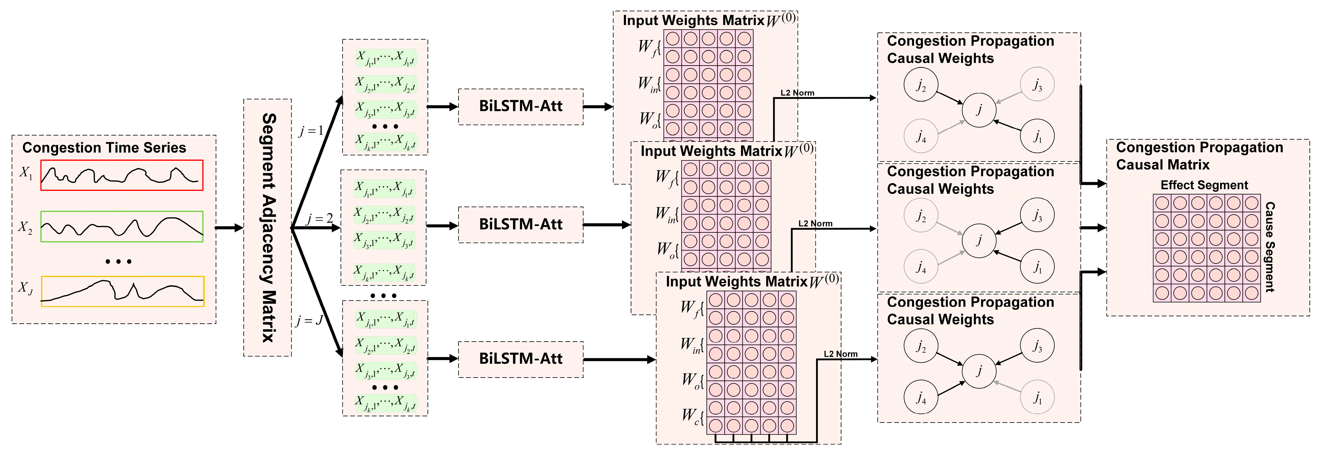
Based on the design proposed above, this paper introduces the Multi-Channel Attention DSNG-BiLSTM model. It employs a Decoupling Causal Architecture to ensure that the influences decouple different input channels, and it incorporates sparse regularization techniques that enable the model to automatically select the input features that contribute significantly to the target output while assigning lower weights to those with lesser contributions. Subsequently, the congestion-propagation causal weight is estimated from the input weight matrix using the following procedure:

Step 1: From the channel ${\mathbb{N}}_j$, select all segments $j_k$ that have been identified as having a causal influence.

Step 2: For each selected segment $j_k$, extract the corresponding column vector $W_{:j_k}^{(0)}$ from $W^{(0)}$.

Step 3: Compute the ${\mathcal{l}}_2$ norm ${‖W_{:j_k}^{(0)}‖}_2$ for each column vector $W_{:j_k}^{(0)}$; the computed value $F_{j_k\to j}$ represents the estimated congestion-propagation causal weight of segment $j_k$ on the target segment $j$.

Based on this process, the corresponding congestion-propagation causal weights can be determined. The specific network architecture is shown in Figure 5.

5. Experiments

This study focuses on a subset of air routes in China’s south-central region. This airspace encompasses three major hub airports—Guangzhou, Wuhan, and Shenzhen—and has the highest flight density in the country. Its complex traffic-flow structure makes rigorous congestion monitoring and control indispensable. We deployed the proposed Multi-Channel Attention DSNG-BiLSTM-Att model in this representative high-load scenario for two objectives. First, it serves to validate the model’s ability to uncover causal relationships governing congestion states and support decisions in high-traffic conditions. Second, it provides controllers with comprehensive situational awareness, enabling a more precise understanding of congestion-propagation mechanisms and timely preventive measures. To ensure the accuracy of congestion state identification and causal inference, boundary waypoints of the original air route network have been merged and pruned, resulting in the simplified topology shown in Figure 6. The experimental dataset comprises radar operation records from 1 May to 7 May 2023—spanning the May Day holiday peak—and thus ensures that our analysis is both representative and reliable.

5.1. Trajectory–Air Route Matching

We first map the aircraft trajectory data to the corresponding air route network structure to compute the selected congestion assessment metrics. However, in actual operations, aircraft do not strictly adhere to the prescribed air route structure and may deviate to a certain extent. Consequently, conventional methods such as point–line matching and vector cross-product techniques may cause a single aircraft to be matched to multiple segments in quick succession, making subsequent congestion assessments inaccurate. To achieve more precise trajectory-to-air route matching, this section proposes a trajectory-segment matching algorithm based on the concept of similarity to search for the optimal air route match. The specific steps are as follows:

Step 1: Classification of Trajectory Point Characteristics.

In the trajectory data, a complete trajectory is composed of multiple trajectory points. To accurately depict the course of the trajectory across different segments, trajectory points are categorized as either turning points or straight-flying points. Let ${\theta }_k$ represent the heading of the k-th trajectory point. When the angular change between five consecutive points and the preceding trajectory point exceeds 10° $|{\theta }_{k+n}-{\theta }_{k+n-5}|>10,n=1,\dots ,5$, the point is considered a turning point, which helps to avoid misclassification due to minor maneuver adjustments. Trajectory points that are not identified as turning points are classified as straight-flying points.

Step 2: Construction of Matching Trajectory Segments.

Since flights typically follow air routes during straight flight, while large angular changes during turns make it challenging to match appropriate segments, all straight-flying trajectory points are extracted. Adjacent sequences of five or more straight-flying trajectory points are then grouped to form a straight trajectory segment. Consequently, a complete flight trajectory is composed of multiple, non-connected straight trajectory segments.

Step3: Construct matching indicators. The similarity metrics constructed in this paper are as follows:

$$similarity={\displaystyle \frac{\overrightarrow{vecto{r}_{segment}}\cdot \overrightarrow{vecto{r}_{flight}}}{\left|\right|\overrightarrow{vecto{r}_{segment}}\left|\right|\cdot \left|\right|\overrightarrow{vecto{r}_{flight}}\left|\right|}}$$

(34)

$$distance=\left|\right|\overrightarrow{vector}-\overrightarrow{vecto{r}_{closest}}\left|\right|$$

(35)

$$proj\_length={\displaystyle \frac{\overrightarrow{vector}\cdot \overrightarrow{vecto{r}_{segment}}}{\overrightarrow{vecto{r}_{segment}}\cdot \overrightarrow{vecto{r}_{segment}}}}$$

(36)

$similarity$ represents the direction vector similarity between the segment and the straight trajectory segment; $distance$ represents the distance between the midpoint of the straight trajectory segment and its nearest projection point on the segment, which characterizes the difference in distance between the trajectory and the segment; $proj\_length$ is the projection position of the nearest projection point of the midpoint of the straight trajectory segment on the segment, which is used to judge whether the track is within the effective projection range of the segment. The screening conditions are as follows:

$$\max similarity+{\displaystyle \frac{1}{distance}}, 0\le proj\_length\le 1$$

(37)

Step 4: Iterative Matching.

The straight trajectory segments are processed in temporal order based on their timestamps. When matching the second and subsequent straight trajectory segments, the corresponding matched segment must be connected to the segment matched in the previous segment. If the matched air route for the current trajectory segment is not connected to the previous one, the distance between the two nearest air route waypoints is examined; if this distance exceeds a predefined threshold $0.1°\times 0.1°$, re-matching is allowed.

When an aircraft is cruising, it may be issued a “direct-to-waypoint” clearance, during which it does not follow any specific segment. To avoid incorrectly assigning such trajectory points to a segment, we delay matching until the aircraft reaches the waypoint and then proceeds along the defined route. Without this check, forced matching during the direct-to phase would produce erroneous congestion estimates. Figure 7 illustrates the effect of this matching algorithm.

5.2. Segment Congestion State Recognition

Based on one week of high-density radar trajectory data collected from 1 May to 7 May 2023, we discretized the data into 10-min intervals, resulting in 1008 time slices. This process produced the congestion state assessment dataset. First, congestion states at waypoints were identified by discretizing the airspace into 7680 grids; then, for each time slice, congestion samples based on the grid partition were generated, accumulating a total of 7,741,440 samples in the dataset. Subsequently, the entropy weight method was employed to calculate the indicator weights for waypoint traffic load, the number of segments, and route-direction entropy, which were determined to be 0.30, 0.36, and 0.34, respectively. Based on these weights, the congestion state assessment values for the waypoints were computed. The figure below displays the computation results for 1 May.

Figure 8 shows the distribution of congested grids in the discretized airspace; color gradients indicate the severity of congestion. By overlaying these grids with waypoint coordinates, specific high-congestion waypoints were identified. Although these waypoints are dispersed throughout the airspace, they cluster mainly in three areas: intersections of air routes, regions surrounding local airports, and the airspace periphery. The waypoints LBN, JW, and LLC each connect to more than eight segments, making them key hubs in the network. UDUMI and DUBAS lie near Wuhan Airport, VIKEB and ISMED near Changsha Airport, and POU near Guangzhou Airport. WXI, BIGRO, XEBUL, and SAMAS are located at the interfaces of different controlled airspace regions, serving as major handover points for cross-airspace traffic.

Subsequently, these waypoints were compared with the waypoints ranked highly in daily traffic flow in the 2023 National Civil Aviation Flight Operations Efficiency Report released by the CAAC. The waypoint data relevant to the target airspace in this study were extracted from the document, as shown in

Table 1. 2023 South-Central Average Daily Traffic Ranking Waypoints.

Ranking	Waypoint	Average Daily Flow	Hourly Peak Flow	Is It Recognized?
1	MAMSI	1014	92	√
2	LLC	999	115	√
3	ISMED	950	105	√
4	PLT	944	97	×
5	DUBAS	924	99	√
6	VIKEB	894	103	√
7	LBN	855	84	√
8	XEBUL	823	73	√
9	POU	795	83	√
10	UDUMI	787	87	√
11	OBDON	780	92	×

.

In the table, the column labeled “Is It Recognized?” indicates whether our method successfully flagged the waypoints that rank highest by daily traffic volume in the CAAC’s reference document as high-congestion points. A comparison shows that the high-congestion waypoints identified by our approach closely match the reference data. Of the eleven waypoints in the south-central region with the highest daily volumes, nine were correctly detected. The remaining two were excluded during network simplification and therefore could not be identified. This result fully validates the effectiveness of our point-and-segment congestion state identification model’s waypoint-level detection component. By accurately capturing each waypoint’s congestion characteristics, this method supplies cross-segment information essential for subsequent segment-level congestion evaluations.

Subsequently, based on the congestion assessment values of the waypoints, we further computed the congestion assessment values for the segments. Using the 1008 predefined time slices and 618 segments within the network, a total of 622,944 samples were generated. After calculating the weights, the weights for segment traffic flow, segment traffic density, aircraft dynamic interaction, and the computed waypoint congestion assessment values were determined to be 0.22, 0.16, 0.46, and 0.16, respectively. After clustering with the FCM-WBO algorithm, the final number of segment samples corresponding to different congestion states is shown in

Table 2. Sample size table for segments.

State	Free	Smooth	Crowded	Jam
Congestion Index	0	1	2	3
Sample Size	436,255	148,110	29,650	8928

.

One of the results of congestion state recognition for the 1 May segment is shown in Figure 9:

Segments in a congested state are predominantly clustered in regions where flow, density, and interaction degree are all high. The primary distinction between segments classified as “Crowded” and those classified as “Smooth” lies in an increase in flow. Furthermore, segments classified as “Free” carry no traffic and hence appear only at the origin of the coordinate axes. To investigate how congestion evolves over time, the proportion of congested segments was computed for various time intervals, as shown in Figure 10.

The figure illustrates how the proportion of segments in each congestion state changes over time. During the early-morning hours, when the number of aircraft is low, the overall airspace congestion state is predominantly free; notably, between midnight and 4:00 a.m., the proportion of Jam and Crowded segments rapidly decreases. With the onset of the early peak period around 7–8 a.m., the proportion of not-free segments rises and then gradually stabilizes. Subsequently, two minor peaks occur between 11:00–13:00 and 17:00–19:00, during which the percentage of free segments slightly declines, and after 19:00, the congestion level of the segments shows a downward trend.

5.3. Generation of Air Route Network Congestion-Propagation Causal Weights

After obtaining the congestion assessment values for the segments, the resulting time series data were then used as inputs and outputs to train the Multi-Channel Attention DSNG-BiLSTM model. Figure 11 shows the model’s loss. As the number of training epochs increases, the loss curve gradually stabilizes, indicating that the model has converged to its optimal parameters.

In order to comprehensively evaluate the performance of the proposed model, we select a series of widely used prediction models as benchmarks for comparison. For all models, a batch size of 10 was set, with each batch containing data from 618 segments, spanning 24-time steps across various time windows. The models were optimized using both the GISTA and ISTA algorithms, and the architectures employed include MLP [44], RNN [45], LSTM [46], and BiLSTM. The parameter settings for the different models are detailed as follows:

All models are fully hyper-parameter-tuned. They are based on $\tau =1$, with a context window of 10, $l{r}_{\min }$ of 1 × 10⁻⁸, $lr\_decay$ of 0.5, and ${\lambda }_1$ and ${\lambda }_2$ of 1 × 10⁻³. The number of hidden layers is 2, the number of neurons in each hidden layer is 64, and the dropout rate is 0.15. The MLP $lr$ is 0.001, and the number of training epochs is 200; the RNN $lr$ is 0.005, the LSTM, BiLSTM, and Multi-Channel Attention DSNG-BiLSTM $lr$ is 0.006, and the number of training epochs is 400. The results of the evaluation metrics are shown in the following table.

Table 3. Combined performance comparison table.

Method		MSE	RMSE	R2
Model	Algorithm
OURS	GISTA	0.0891	0.2343	0.9161
	ISTA	0.1166	0.3416	0.8854
BiLSTM	GISTA	0.1082	0.2689	0.8952
	ISTA	0.1271	0.3579	0.8805
LSTM	GISTA	0.1146	0.2835	0.8891
	ISTA	0.1333	0.3651	0.8705
RNN	GISTA	0.1553	0.3327	0.8498
	ISTA	0.1912	0.4373	0.8147
MLP	GISTA	0.2465	0.4864	0.7659
	ISTA	0.2587	0.5087	0.7479

shows that, compared with the RNN and MLP models, the LSTM model reduced the RMSE by 35% and 44%, respectively, demonstrating its superior capability in capturing long-term dependencies in time series and handling complex dynamic. Moreover, the BiLSTM model further enhances the accuracy of congestion-propagation causal weight estimation through bidirectional information modeling, outperforming the unidirectional LSTM. Among the four models compared, the proposed model demonstrates the best performance. The introduction of the self-attention mechanism allows it to more accurately reflect the congestion characteristics of segments, with improvements over BiLSTM in MSE, RMSE, and R² of 17.6%, 12.9%, and 2.3%, respectively. Additionally, significant performance differences were observed when comparing models optimized using the GISTA algorithm to those using the ISTA algorithm, suggesting that adaptive step size adjustment through linear search leads to more reasonable parameter updates, faster convergence, and reduced oscillations.

5.4. Analysis of the Spatial Characteristics of Congestion Propagation in Air Route Networks

In an air route network, congestion propagation can be regarded as the continual diffusion of congestion information along the directed links between segments. After training a deep causal learning model on historical flight-operation data, the resulting causal weight $F_{j_k\to j}$ precisely captures the latent likelihood that segment $j_k$ will transmit congestion information to its neighboring segment j. Because this weight quantifies propagation capability, we refer to it as the CPP, defined as follows:

$${\mathrm{CPP}}_{j_k\to j}=F_{j_k\to j}$$

(38)

When ${\mathrm{CPP}}_{j_k\to j}>0$, it indicates that when segment $j_k$ becomes congested, it transmits congestion to its adjacent segment j; the higher the CPP value, the more pronounced segment influence on the congestion state of its neighbors. If ${\mathrm{CPP}}_{j_k\to j}<0$, it means that segment $j_k$ is affected by congestion propagation from segment j. When ${\mathrm{CPP}}_{j_k\to j}=0$, there is no causal relationship of congestion propagation between the two segments.

To accurately reveal the roles and mutual interactions of segments in the congestion-propagation process, a complex network model based on CPP is constructed. It introduces the eigenvector centrality metric, which not only measures the connection strength between a node and its direct neighbors but also reflects the indirect associations between that node and other high-impact nodes in the entire network. A higher eigenvector centrality value indicates that the segment plays a more pivotal role in congestion propagation. Quantifying this metric can help identify key nodes in the congestion diffusion process. Based on this analytical framework, we systematically analyze both the topological structure of the original air route network and the topology of the CPP network constructed under different time-lag conditions. The identification results are presented in

Table 4. Eigenvector centrality results.

Air Route Network		$\mathbf{CPP} \mathbf{Network} \mathit{\tau }=1$		$\mathbf{CPP} \mathbf{Network} \mathit{\tau }=2$		$\mathbf{CPP} \mathbf{Network} \mathit{\tau }=3$
Segment	Value	Segment	Value	Segment	Value	Segment	Value
IDUMA-BEKOL	0.262	LLC-OKIXA	0.317	LLC-PUKAD	0.342	LLC-OKIXA	0.314
IDUMA-SHL	0.262	LLC-SANES	0.312	BEMTA-LLC	0.322	LLC-PUKAD	0.314
SHL-IDUMA	0.257	LLC-PUKAD	0.307	LLC-SANES	0.314	LLC-XOPEK	0.307
SHL-P436	0.257	LLC-XOPEK	0.298	LLC-OKIXA	0.311	BEMTA-LLC	0.302
SHL-NUSLA	0.257	LLC-W	0.284	LLC-XOPEK	0.293	LLC-SANES	0.292

.

Figure 12 shows the detailed visualization results.

In the analysis of the air route network, we found that major hubs are concentrated in segments near Guangzhou; however, in the CPP networks constructed under different time lags, the key nodes are primarily located in segments adjacent to the LLC waypoint. This is because in the air route network, all edge weights are set to 1, and the segments in the Guangzhou area are densely connected, resulting in a network structure with high complexity that is more readily identified as key hubs. In contrast, in the CPP network, the edge weights are set to the corresponding CPP values. Although the network structure near the LLC is relatively simple, it is still identified as a hub in the congestion-propagation process, indicating that the congestion effect in the LLC area can rapidly diffuse to surrounding segments. Furthermore, CPP networks across different time lags consistently highlight the same LLC-adjacent segments as central, showing that the LLC area retains its pivotal role in congestion propagation throughout central-southern China regardless of the chosen lag.

Although the CPP quantifies a segment’s latent ability to transmit congestion to its adjacent segments, it does not capture the actual directionality and intensity distribution observed during real-world propagation. To address this limitation, we introduce a new metric: the CPF. In physics, flux is typically defined as the net flow per unit time through a given surface. By analogy, CPF characterizes both the direction and the magnitude of congestion transfer at various time lags by measuring the relative differences between CPP values of different segments. Mathematically, CPF is defined as:

$${\mathrm{CPF}}_{j_k\to j}={\mathrm{CPP}}_{j_k\to j}-{\mathrm{CPP}}_{j\to j_k}$$

(39)

When ${\mathrm{CPF}}_{j_k\to j}>0$, it indicates that congestion is actually transmitted from segment $j_k$ to segment j, and the magnitude of it reflects the amount of congestion being transferred. If ${\mathrm{CPF}}_{j_k\to j}<0$, it indicates that congestion is primarily transmitted from segment j to segment $j_k$. When ${\mathrm{CPF}}_{j_k\to j}=0$, it signifies that no congestion-propagation relationship exists between the two segments.

The CPF network is further constructed to reflect the actual propagation patterns of congestion among segments. To deeply analyze the main propagation paths of congestion in the air route network, betweenness centrality is employed. Betweenness centrality measures the role of a node as a “bridge” within the network by calculating the frequency with which it appears on all shortest paths. In this study, a segment with high betweenness centrality indicates that it connects different regions and accelerates the diffusion of localized congestion to a wider area. Based on this approach, the betweenness centrality of the CPF networks under different time lags was computed, with the specific results in

Table 5. Betweenness centrality results.

Air Route Network		$\mathbf{CPF} \mathbf{Network} \mathit{\tau }=1$		$\mathbf{CPF} \mathbf{Network} \mathit{\tau }=2$		$\mathbf{CPF} \mathbf{Network} \mathit{\tau }=3$
Segment	Value	Segment	Value	Segment	Value	Segment	Value
P285-UQN	0.238	CD-KALMU	0.093	MOLSO-YIN	0.196	LIN-NOMUK	0.072
UQN-BUBDA	0.231	HEN-LLC	0.092	BEMAG-LLC	0.188	KALMU-LIN	0.072
MOLSO-P285	0.226	LLC-P375	0.091	P419-YIN	0.187	CD-LIN	0.070
YIN-MOLSO	0.215	DODSA-LLC	0.091	LLC-W	0.186	CD-XOPEK	0.068
OBDON-REPUV	0.145	CD-NOMUK	0.086	POU-TEPID	0.134	JW-MUBEL	0.067

.

Figure 13 shows the detailed visualization results.

In the air route network shown in Figure 13a, “trunk” routes such as W56, W45, and V107, which run north–south through the entire Central South airspace, exhibit high betweenness centrality—consistent with the fact that a large volume of traffic follows these primary corridors. At $\tau =1$ and $\tau =2$, congestion propagates principally through waypoints CD, LLC, PUNIR, and POU along a northwest–southeast axis between the Guangzhou and Changsha control sectors. When the time lag increases to $\tau =2$, congestion additionally spreads via waypoints LIN, WTM, and LKO into the Wuhan airspace, and subsequently diffuses along the main north–south route W56. At $\tau =3$, the congestion-propagation path shifts noticeably toward the western portion of the network, following waypoints POU, JW, YIH, and LIN to form a south-to-north propagation channel, indicating a concentration of congestion in the western region. During this stage, LLC no longer serves as a primary propagation node, suggesting that most eastern routes have already experienced congestion during earlier lags, and that western routes have become the dominant channels for further congestion diffusion at longer lags.

Since the early congestion pathways primarily connected core areas with high air traffic density—such as Guangzhou Airport, the LLC waypoint, Changsha Airport, and Wuhan Airport—it can be inferred that initial congestion propagation originated in these regions. These core areas not only concentrate significant air traffic but also possess strong connectivity within the air route network. Consequently, once congestion occurs, it can rapidly impact the routes linking other airspaces, further exacerbating the spread of congestion.

After a detailed analysis of the congestion-propagation pathways, our focus shifts to the sources of congestion. To this end, we introduce out-degree centrality as a key metric. Out-degree centrality reflects a node’s capability to directly transmit information or effects to others. In the CPF network, segments with high out-degree centrality can rapidly convey congestion signals to numerous adjacent segments, thereby serving as primary origins of congestion propagation; accordingly, they can effectively identify the nodes most likely to trigger congestion spread. We conducted a similar analysis for all four types of networks. The results are presented in

Table 6. Out-degree centrality results.

Air Route Network		$\mathbf{CPF} \mathbf{Network} \mathit{\tau }=1$		$\mathbf{CPF} \mathbf{Network} \mathit{\tau }=2$		$\mathbf{CPF} \mathbf{Network} \mathit{\tau }=3$
Segment	Value	Segment	Value	Segment	Value	Segment	Value
GYA-POU	0.010	NLG-SAREX	0.003	GLN-ZAO	0.003	ANPIM-DOBVI	0.004
MUBEL-POU	0.010	VANPI-W	0.003	EPGOS-RUMGU	0.003	K-SHL	0.003
CON-POU	0.010	URGEB-XSH	0.002	DYL-P548	0.003	P192-P281	0.003
TEPID-POU	0.010	DYL-P548	0.002	AGTEL-WCF	0.003	DHP-P38	0.003
NOMAR-POU	0.010	GLN-ZAO	0.002	H-HG	0.003	NNX-UQN	0.003

.

Figure 14 shows the detailed visualization results.

Figure 14 maps congestion-source segments in the Central and Southern regions under three time-lag conditions. In the original air route topology, segments with high out-degree centrality cluster mainly around waypoints LLC, POU, LBN, ZUH, and WHA and their adjacent airspace. When $\tau =1$, these same areas dominate as congestion sources, indicating that short-term propagation primarily originates there. As $\tau =2$, the spatial concentration remains similar, but the intensity of influence on neighboring segments diminishes—as reflected by lighter shading in the heatmap. At $\tau =3$, the prominence of LLC, POU, and WHA further declines, and congestion sources begin to shift toward shorter, east-west-oriented segments. This shift is consistent with the initial congestion origins identified in earlier analyses.

The spatial distribution characteristics of congestion sources vary markedly under different time lag conditions. At short time lags, congestion sources are typically concentrated around airports or near major air route intersections; however, their source effects diminish significantly over longer time lags, and the surrounding areas gradually become the primary sources of congestion. This indicates that as the propagation time lag increases, congestion sources are no longer confined to the initial outbreak cores but instead diffuse across the entire network, resulting in a more dispersed spatial distribution.

Based on preliminary analysis, this study identified congestion sources in the air route network that exhibit high propagation capabilities. Next, these key segments are combined with their respective congestion assessment values to verify whether high out-degree centrality corresponds to more severe local congestion. Data for the top 10% of segments with the highest out-degree centrality were selected for investigation, as shown in Figure 15.

In this graph, it is observed that segments with high out-degree centrality—acting as congestion-propagation sources—exhibit an average congestion assessment value concentrated between 0.023 and 0.038, a level that did not reach “Jam” state in the previous congestion state identification. On the other hand, although these segments account for only 10% of all segments, they propagate 40.42% of the total congestion in the network. This phenomenon arises because these segments connect to others that can rapidly accommodate or absorb congestion. Consequently, whenever these segments begin to show a congestion trend, even though their own congestion state is not severe, they quickly disseminate congestion signals.

In Figure 16, we conducted a systematic analysis of congestion-propagation characteristics on the adjacent segments of each identified congestion source. For each source segment, the neighboring segment with the highest in-degree centrality was selected as its representative. The results indicate that 69.81% of these representative segments were classified as “Jam” in the congestion states assessment. Moreover, each of these segments exhibited an in-degree centrality exceeding 0.001, placing them within the top 24.93% of all segments in the air route network. This finding demonstrates that a substantial portion of congestion signals emanating from source segments converge on these high-centrality neighbors, making them critical nodes for receiving and redistributing congestion information. Based on this insight, we introduce the concept of “potential burdened segments” to denote segments that function as key reception nodes during congestion diffusion. We adopt an in-degree centrality threshold of 0.001 to identify such segments. Given their pivotal role in bearing latent congestion pressure, air traffic control authorities should prioritize monitoring these segments and implement real-time interventions upon detecting early signs of congestion at their upstream source nodes, thereby preventing further amplification and spread of network-wide congestion.

5.5. Analysis of the Temporal Characteristics of Congestion Propagation in Air Route Networks

After thoroughly investigating the spatial relationships of congestion propagation in the air route network under different time lags, the analysis then shifts toward the temporal dimension. By comparing the variations in CPP and CPF over time, the dynamic characteristics of congestion propagation across different time periods can be deeply analyzed, thereby revealing the temporal propagation patterns of congestion. For example, the segment pair GYA-POU and POU-YIN serve as a typical analysis object because both are connected to numerous other segments and have a significant impact on the stability and operational efficiency of the entire air route network. The specific structure is shown in Figure 17.

Taking GYA-POU and POU-YIN as examples, we analyze the CPP between these segments. As shown in Figure 18, during the early-morning hours, the CPP is significantly low due to reduced traffic volume, and the system remains relatively stable. At 8:00, a pronounced peak emerges; notably, the curve for $\tau =3$ reaches its highest value, and the peak values for $\tau$ 1, 2, and 3 gradually increase. This suggests that during peak periods, congestion not only intensifies over time but also diffuses more broadly, as evidenced by a marked increase in propagation potential.

The relationship between the CPP of the segment and the congestion assessment value is further explored in conjunction with the congestion assessment value of the segment assessed in the previous section, as shown in Figure 19:

As shown in Figure 19, the purple line represents the linear fitting equation. Correlating CPP with congestion state evaluation values reveals two distinct clusters of sample points: one cluster exhibits low values for both metrics, while the other exhibits high values for both. Between these clusters, a sharp discontinuity appears—CPP jumps directly from 0.02 to 0.15 without a gradual transition. This abrupt change indicates that once traffic flow complexity increases beyond a certain critical threshold, the congestion-propagation effect across the air route network rapidly amplifies, thereby confirming that causal relationships strengthen significantly during peak periods.

Afterward, to deeply understand the interactions between segments and the congestion-propagation effect, the CPF between pairs of segments is analyzed to explore the congestion-propagation characteristics between segments under different time lags. Since the direction of transmission is not discussed here for the time being, absolute values are taken for treatment. Take the CPF between GYA-POU and POU-YIN as an example, as shown in Figure 20:

Figure 20 shows that during the early-morning period (00:00–04:00), the CPF for $\tau =1$ is relatively high, and the differences among various time-lag intervals are small, indicating that when traffic volume is low, congestion dissipates rapidly. In contrast, during peak hours (e.g., 11:00–13:00), the variance among time-lag differences increases, with the propagation effect being strongest at $\tau =3$, and the time required for congestion to spread significantly lengthens. This pattern demonstrates that as traffic volume rises, the time needed for congestion effects to manifest increases. This phenomenon further suggests that during peak periods, air traffic control units typically implement mitigation measures, which extend the propagation duration and slow the speed of congestion spread.

After completing the analysis between a single pair of segments, we extend our investigation to the CPF of the entire air route network, where the CPF of the air route network is defined as the average of the CPF of all the pairs of segments at that moment in time. This is demonstrated in Figure 21.

As shown, during both the pre-dawn hours and the peak period, the patterns closely mirror those in Figure 20, consistent with the previously established congestion-propagation dynamics. Specifically, as afternoon-peak congestion gradually dissipates, the CPF value for $\tau =3$ steadily decreases and eventually falls below those of $\tau =1$ and $\tau =2$, reflecting a transition toward off-peak characteristics and confirming the propagation behavior described earlier.

Based on the above findings, we conducted a comparative analysis of congestion-propagation speeds during different time periods. We compared congestion-propagation speeds across three intervals: 00:00–04:00 (low-traffic) and the two peak periods 07:00–09:00 and 11:00–13:00. For each interval, we computed the propagation speed by first measuring the time lag between when adjacent segments became congested. We then defined propagation distance as half the average length of those two segments. Dividing distance by time lag yielded the propagation speed.

Table 7. Congestion-propagation speed results.

Time Period	Average Congestion-Propagation Speed (km/h)	Average Congestion Propagation Time (min)
0–4 h	163.53	15.71
7–9 h	108.85	23.22
11–13 h	97.46	27.29

summarizes the average speeds: peak-hour speeds are 36.92% lower than those in the low-traffic interval. This slower spread during peak hours indicates that controller interventions effectively reduce its propagation.

6. Conclusions

This study aimed to estimate the causal weights of congestion propagation within the air route network and, by comparing spatiotemporal characteristics under varying time-lag conditions, to develop a cross-segment congestion-propagation causal lag analysis framework. (1) We constructed a point–line congestion assessment model that accounts for cross-segment interactions between aircraft, and introduced the FCM-WBO algorithm—based on the entropy weight method and the White Whale Optimization algorithm—to accurately identify each segment’s congestion status. (2) We built upon this foundation by designing the Multi-Channel Attention DSNG-BiLSTM-Att model to estimate causal weights of congestion propagation between segments. (3) We categorized congestion time lags into three levels and, in the spatial dimension, constructed CPP and CPF networks corresponding to each lag level—extracting key metrics to reveal spatial propagation patterns—while, in the temporal dimension, analyzing differences in CPP and CPF across various periods and lag levels to characterize congestion-propagation dynamics over time.

The findings reveal that congestion propagation exhibits distinctly different features under various time lag conditions. Spatially, at low time lags, congestion sources tend to be concentrated around airports or near major air route intersections. As time lags increase, the congestion sources shift to shorter, east–west-oriented segments. Overall, although these congestion source segments themselves exhibit relatively low congestion levels (ranging from 0.023 to 0.038), they can rapidly transmit slight congestion signals to adjacent segments—indeed, the top 10% of segments with the highest propagation effects account for 40.42% of the overall congestion. Based on the propagation characteristics of the segments adjacent to these sources, the concept of potential burdened segments is introduced to designate key receiving nodes. Temporally, during off-peak early-morning hours when traffic volume is lower, the CPP is relatively low, and congestion propagates rapidly, reaching speeds of up to 163.53 km/h and completing within approximately 15 min. In contrast, during peak periods, once the congestion assessment value of a segment reaches a critical threshold of about 0.05, the CPP abruptly rises to 0.15. Simultaneously, due to air traffic control interventions, the average propagation speed is reduced by 36.92%, and the full effect of congestion takes longer to manifest.

The findings of this study enable air traffic control authorities to enhance their situational awareness of congestion evolution within the air route network and to intervene more effectively. On the one hand, CPP and CPF risk heatmaps, along with the corresponding causal weight matrices, can be displayed on controllers’ monitoring interfaces to provide real-time risk alerts, thereby allowing them to quantitatively assess the effectiveness of countermeasures such as staggered departures and rerouted flow restrictions. On the other hand, the long-term accumulation of congestion-propagation patterns can be incorporated into simulator training to reproduce multi-lag evolution processes. Furthermore, these empirically derived propagation insights can retroactively calibrate air route topology and flow-management strategies, furnishing data-driven support for fine-grained airspace management and ongoing optimization.

However, there are several limitations in this study that warrant further exploration. First, the proposed method primarily relies on training with historical radar data, yet in actual operations, factors such as adverse weather conditions and unexpected events also impact congestion in the air route network. Future research could incorporate these uncertainties into the model to further enhance its robustness. Second, the selection of key hyperparameters in the model still relies primarily on empirical judgment and thus remains somewhat subjective; yet there is no adaptive-optimization or data-driven approach available to dynamically calibrate these parameters. Lastly, this study only examines the propagation characteristics of congestion. Future work could develop specific congestion mitigation and optimization strategies to provide intelligent decision-making support for air traffic controllers.

References

1. Huang, X.; Tian, Y.; Li, J.; Zhang, N.; Dong, X.; Lv, Y.; Li, Z. Joint Autonomous Decision-Making of Conflict Resolution and Aircraft Scheduling Based on Triple-Aspect Improved Multi-Agent Reinforcement Learning. Expert Syst. Appl. 2025, 275, 127024. [Google Scholar] [CrossRef]
2. Bowen, J.T. The Economic Geography of Air Transport. In The Geographies of Air Transport; Routledge: London, UK, 2016; pp. 41–60. [Google Scholar]
3. Sismanidou, A.; Tarradellas, J.; Suau-Sanchez, P. The Uneven Geography of US Air Traffic Delays: Quantifying the Impact of Connecting Passengers on Delay Propagation. J. Transp. Geogr. 2022, 98, 103260. [Google Scholar] [CrossRef]
4. Sun, M.; Tian, Y.; Wang, X.; Huang, X.; Li, Q.; Li, Z.; Li, J. Transport Causality Knowledge-Guided GCN for Propagated Delay Prediction in Airport Delay Propagation Networks. Expert Syst. Appl. 2024, 240, 122426. [Google Scholar] [CrossRef]
5. Zhao, Z.; Yuan, J.; Liu, Y. Research and Comparison on Identification and Prediction Methods of Air Traffic Network Congestion. In Proceedings of the 2022 4th International Academic Exchange Conference on Science and Technology Innovation (IAECST), Guangzhou, China, 9–11 December 2022; pp. 1256–1264. [Google Scholar]
6. Stopher, P.R. Reducing Road Congestion: A Reality Check. Transp. Policy 2004, 11, 117–131. [Google Scholar] [CrossRef]
7. Greenshields, B.D.; Bibbins, J.R.; Channing, W.; Miller, H.H. A Study of Traffic Capacity. In Proceedings of the Highway Research Board Proceedings, Washington, DC, USA, 6–7 December 1935; Volume 14, pp. 448–477. [Google Scholar]
8. Kumar, N.; Raubal, M. Applications of Deep Learning in Congestion Detection, Prediction and Alleviation: A Survey. Transp. Res. Part C Emerg. Technol. 2021, 133, 103432. [Google Scholar] [CrossRef]
9. Lin, Y.; Li, L.; Ren, P.; Wang, Y.; Szeto, W.Y. From Aircraft Tracking Data to Network Delay Model: A Data-Driven Approach Considering En-Route Congestion. Transp. Res. Part C Emerg. Technol. 2021, 131, 103329. [Google Scholar] [CrossRef]
10. Wu, W.; Zhang, H.; Feng, T.; Witlox, F. A Network Modelling Approach to Flight Delay Propagation: Some Empirical Evidence from China. Sustainability 2019, 11, 4408. [Google Scholar] [CrossRef]
11. Puechmorel, S. Air Traffic Complexity: Towards Intrinsic Metrics. In Proceedings of the 3rd USA/Europe Air Traffic Management R&D Seminar, Napoli, Italy, 13–16 June 2000. [Google Scholar]
12. Wang, H.; Huang, J.; Deng, T.; Song, Z. Evaluation and Optimization of Air Traffic Complexity Based on Resilience Metrics. J. Adv. Transp. 2023, 2023, 5692934. [Google Scholar] [CrossRef]
13. Li, S.; Wang, C.; Wang, J. Exploring Dynamic Characteristics of Multi-State Air Traffic Flow: A Time Series Approach. IEEE Access 2020, 8, 64565–64577. [Google Scholar] [CrossRef]
14. Jiang, X.; Wen, X.; Wu, M.; Song, M.; Tu, C. A Complex Network Analysis Approach for Identifying Air Traffic Congestion Based on Independent Component Analysis. Phys. Stat. Mech. Its Appl. 2019, 523, 364–381. [Google Scholar] [CrossRef]
15. Yan, Y.; Zhang, S.; Tang, J.; Wang, X. Understanding Characteristics in Multivariate Traffic Flow Time Series from Complex Network Structure. Phys. Stat. Mech. Its Appl. 2017, 477, 149–160. [Google Scholar] [CrossRef]
16. Chen, X.W.; Landry, S.J.; Nof, S.Y. A Framework of Enroute Air Traffic Conflict Detection and Resolution through Complex Network Analysis. Comput. Ind. 2011, 62, 787–794. [Google Scholar] [CrossRef]
17. Hongyong, W.; Ruiying, W.; Yifei, Z. Analysis of Topological Characteristics in Air Traffic Situation Networks. Proc. Inst. Mech. Eng. Part G J. Aerosp. Eng. 2015, 229, 2497–2505. [Google Scholar] [CrossRef]
18. Chen, H.; Zhou, Z.; Wu, L.; Fu, Y.; Xue, D. Enhancing Air Traffic Complexity Assessment through Deep Metric Learning: A CNN-Based Approach. Aerosp. Sci. Technol. 2025, 160, 110090. [Google Scholar] [CrossRef]
19. Ji, Y.; Yu, F.; Shen, D.; Peng, Y. Study on the Identification of Terminal Area Traffic Congestion Situation Based on Symmetrical Random Forest. Symmetry 2025, 17, 96. [Google Scholar] [CrossRef]
20. Berrouk, S.; Fazziki, A.E.; Sadgal, M. Fuzzy-Based Approach for Assessing Traffic Congestion in Urban Areas. In Proceedings of the Image and Signal Processing: 9th International Conference, ICISP 2020, Marrakesh, Morocco, 4–6 June 2020; Proceedings 9. Springer: Berlin/Heidelberg, Germany, 2020; pp. 112–121. [Google Scholar]
21. Gilbo, E.P.; Smith, S.B. New Method for Probabilistic Traffic Demand Predictions for En Route Sectors Based on Uncertain Predictions of Individual Flight Events. In Proceedings of the Ninth USA/Europe Air Traffic Management Research and Development Seminar (ATM2011), Berlin, Germany, 14–17 June 2011. [Google Scholar]
22. Zhang, H.; Jiang, C.; Yang, L. Forecasting Traffic Congestion Status in Terminal Areas Based on Support Vector Machine. Adv. Mech. Eng. 2016, 8, 1687814016667384. [Google Scholar] [CrossRef]
23. Kumar, M.; Kumar, K. Traffic Congestion Prediction Using Feature Series LSTM Neural Network and a New Congestion Index. Int. J. Artif. Intell. Tools 2024, 33, 2350067. [Google Scholar] [CrossRef]
24. Rahman, R.; Hasan, S. Real-Time Signal Queue Length Prediction Using Long Short-Term Memory Neural Network. Neural Comput. Appl. 2021, 33, 3311–3324. [Google Scholar] [CrossRef]
25. Chawla, N.; Wang, W. Proceedings of the 2017 SIAM International Conference on Data Mining; SIAM: Philadelphia, PA, USA, 2017. [Google Scholar]
26. Liu, Y.; Zheng, H.; Feng, X.; Chen, Z. Short-Term Traffic Flow Prediction with Conv-LSTM. In Proceedings of the 2017 9th International Conference on Wireless Communications and Signal Processing (WCSP), Nanjing, China, 11–13 October 2017; IEEE: Hoboken, NJ, USA, 2017; pp. 1–6. [Google Scholar]
27. Wu, C.; Ding, H.; Fu, Z.; Sun, N. Air Traffic Flow Prediction in Aviation Networks Using a Multi-Dimensional Spatiotemporal Framework. Electronics 2024, 13, 3803. [Google Scholar] [CrossRef]
28. Shen, Z.; Cai, K.; Fang, Q.; Luo, X. Air Traffic Flow Prediction with Spatiotemporal Knowledge Distillation Network. J. Adv. Transp. 2024, 2024, 4349402. [Google Scholar] [CrossRef]
29. Hammerton, G.; Munafò, M.R. Causal Inference with Observational Data: The Need for Triangulation of Evidence. Psychol. Med. 2021, 51, 563–578. [Google Scholar] [CrossRef] [PubMed]
30. Raita, Y.; Camargo Jr, C.A.; Liang, L.; Hasegawa, K. Big Data, Data Science, and Causal Inference: A Primer for Clinicians. Front. Med. 2021, 8, 678047. [Google Scholar] [CrossRef] [PubMed]
31. Runge, J.; Gerhardus, A.; Varando, G.; Eyring, V.; Camps-Valls, G. Causal Inference for Time Series. Nat. Rev. Earth Environ. 2023, 4, 487–505. [Google Scholar] [CrossRef]
32. Zeng, L.; Wang, B.; Wang, T.; Wang, Z. Research on Delay Propagation Mechanism of Air Traffic Control System Based on Causal Inference. Transp. Res. Part C Emerg. Technol. 2022, 138, 103622. [Google Scholar] [CrossRef]
33. He, P.; Sun, R. Trend Analysis of Civil Aviation Incidents Based on Causal Inference and Statistical Inference. Aerospace 2023, 10, 822. [Google Scholar] [CrossRef]
34. Li, C.; Liu, W.; Yang, H. Deep Causal Inference for Understanding the Impact of Meteorological Variations on Traffic. Transp. Res. Part C Emerg. Technol. 2024, 165, 104744. [Google Scholar] [CrossRef]
35. Kang, J.; Yang, S.; Shan, X.; Bao, J.; Yang, Z. Exploring Delay Propagation Causality in Various Airport Networks with Attention-Weighted Recurrent Graph Convolution Method. Aerospace 2023, 10, 453. [Google Scholar] [CrossRef]
36. Zhu, Q.; Chen, S.; Guo, T.; Lv, Y.; Du, W. A Spatio-Temporal Approach with Self-Corrective Causal Inference for Flight Delay Prediction. IEEE Trans. Intell. Transp. Syst. 2024, 25, 20820–20831. [Google Scholar] [CrossRef]
37. Tan, J.; Zhao, H.; Yang, R.; Liu, H.; Li, S.; Liu, J. An Entropy-Weighting Method for Efficient Power-Line Feature Evaluation and Extraction from Lidar Point Clouds. Remote Sens. 2021, 13, 3446. [Google Scholar] [CrossRef]
38. Zhong, C.; Li, G.; Meng, Z. Beluga Whale Optimization: A Novel Nature-Inspired Metaheuristic Algorithm. Knowl.-Based Syst. 2022, 251, 109215. [Google Scholar] [CrossRef]
39. Shojaie, A.; Fox, E.B. Granger Causality: A Review and Recent Advances. Annu. Rev. Stat. Its Appl. 2022, 9, 289–319. [Google Scholar] [CrossRef] [PubMed]
40. Tank, A.; Covert, I.; Foti, N.; Shojaie, A.; Fox, E.B. Neural Granger Causality. IEEE Trans. Pattern Anal. Mach. Intell. 2021, 44, 4267–4279. [Google Scholar] [CrossRef] [PubMed]
41. Siami-Namini, S.; Tavakoli, N.; Namin, A.S. The Performance of LSTM and BiLSTM in Forecasting Time Series. In Proceedings of the 2019 IEEE International Conference on Big Data (Big Data), Los Angeles, CA, USA, 9–12 December 2019; IEEE: Hoboken, NJ, USA, 2019; pp. 3285–3292. [Google Scholar]
42. Vaswani, A.; Shazeer, N.; Parmar, N.; Uszkoreit, J.; Jones, L.; Gomez, A.N.; Kaiser, Ł.; Polosukhin, I. Attention Is All You Need. Adv. Neural Inf. Process. Syst. 2017, 30, 6000–6010. [Google Scholar]
43. Daubechies, I.; Defrise, M.; De Mol, C. An Iterative Thresholding Algorithm for Linear Inverse Problems with a Sparsity Constraint. Commun. Pure Appl. Math. J. Issued Courant Inst. Math. Sci. 2004, 57, 1413–1457. [Google Scholar] [CrossRef]
44. Rumelhart, D.E.; Hinton, G.E.; Williams, R.J. Learning Representations by Back-Propagating Errors. Nature 1986, 323, 533–536. [Google Scholar] [CrossRef]
45. Elman, J.L. Finding Structure in Time. Cogn. Sci. 1990, 14, 179–211. [Google Scholar] [CrossRef]
46. Hochreiter, S.; Schmidhuber, J. Long Short-Term Memory. Neural Comput. 1997, 9, 1735–1780. [Google Scholar] [CrossRef]
Figure 1. Point–line congestion assessment model.
Aerospace 12 00529 g001
Figure 2. Congestion state assessment indicators.
Aerospace 12 00529 g002
Figure 3. Flowchart of FCM-WBO algorithm.
Aerospace 12 00529 g003
Figure 4. BiLSTM structure.
Aerospace 12 00529 g004
Figure 5. Multi-Channel Attention DSNG-BiLSTM network architecture.
Aerospace 12 00529 g005
Figure 6. Structure of the air route network.
Aerospace 12 00529 g006
Figure 7. Schematic diagram of trajectory-segment matching results.
Aerospace 12 00529 g007
Figure 8. Results of the congestion state assessment for waypoints.
Aerospace 12 00529 g008
Figure 9. Segment congestion state recognition results.
Aerospace 12 00529 g009
Figure 10. Percentage of congested state of air route network.
Aerospace 12 00529 g010
Figure 11. Loss function variation graph.
Aerospace 12 00529 g011
Figure 12. Eigenvector centrality heatmaps. (a) Air route network eigenvector centrality results; (b) τ = 1 CPP network eigenvector centrality results; (c) τ = 2 CPP network eigenvector centrality results; (d) τ = 3 CPP network eigenvector centrality results.
Aerospace 12 00529 g012aAerospace 12 00529 g012b
Figure 13. Betweenness centrality heatmaps. (a) Air route network betweenness centrality results; (b) τ = 1 CPF network betweenness centrality results; (c) τ = 2 CPF network betweenness centrality results; (d) τ = 3 CPF network betweenness centrality results.
Aerospace 12 00529 g013
Figure 14. Out-degree centrality heatmaps. (a) Air route network out-degree centrality results; (b) τ = 1 CPF network out-degree centrality results; (c) τ = 2 CPF network out-degree centrality results; (d) τ = 3 CPF network out-degree centrality results.
Aerospace 12 00529 g014aAerospace 12 00529 g014b
Figure 15. Average segment congestion assessment value vs. Out-degree centrality.
Aerospace 12 00529 g015
Figure 16. In-degree centrality distribution of selected segments.
Aerospace 12 00529 g016
Figure 17. GYA-POU and POU-YIN structure.
Aerospace 12 00529 g017
Figure 18. CPP between GYA-POU and POU-YIN.
Aerospace 12 00529 g018
Figure 19. Segment congestion assessment value vs. CPP.
Aerospace 12 00529 g019
Figure 20. CPF between GYA-POU and POU-YIN.
Aerospace 12 00529 g020
Figure 21. CPF in air route network.
Aerospace 12 00529 g021