A Procedure for Developing a Flight Mechanics Model of a Three-Surface Drone Using Semi-Empirical Methods

Abstract

Aircraft and fixed-wing drones, designed to perform vertical take-off and landing (VTOL), often incorporate unconventional configurations that offer unique capabilities but simultaneously pose significant challenges in flight mechanics modeling, whose reliability strongly depends on the correct tuning of the inertial and aerodynamic parameters. Having a good characterization of the aerodynamics represents a critical issue, especially in the design and optimization of unconventional aircraft configurations, when, indeed, one is bound to employ empirical or semi-empirical methods, devised for conventional geometries, that struggle to capture complex aerodynamic interactions. Alternatives such as high-fidelity computational fluid dynamics (CFD) simulations, although more accurate, are typically expensive and impractical for both preliminary design and lofting optimization. This work introduces a procedure that exploits multiple analyses conducted through semi-empirical methodologies implemented in the USAF Digital DATCOM to develop a flight mechanics model for fixed-wing unmanned aerial vehicles (UAVs). The reference UAV chosen to test the proposed procedure is the Dragonfly DS-1, an electric VTOL UAV developed by Overspace Aviation, featuring a three-surface configuration. The accuracy of the polar data, i.e., the lift and drag coefficients, is assessed through comparisons with computational fluid dynamics simulations and flight data. The main discrepancies are found in the drag estimation. The present work represents a preliminary investigation into the possible extension of semi-empirical methods, consolidated for traditional configurations, to unconventional aircraft so as to support early-stage UAV design.

1. Introduction

Often, the design of fixed-wing drones features highly innovative configurations that are devised to enable vertical take-off and landing (VTOL) capabilities while also offering superior endurance and efficiency compared to standard multicopters. In this context, designing and optimizing such unusual configurations pose an inherent challenge: semi-empirical methods may not provide adequate aerodynamic characterization due to the unique features of unconventional designs, but advanced computational methods, such as computational fluid dynamics (CFD), have a high computational cost, making them impractical for early-stage design and iterative optimization. Vortex lattice and panel methods [1] may represent a good balance between computational cost and the quality of predictions, but they suffer from some limitations related to the viscous drag and the modeling of body–wing interaction.

Notwithstanding this inherent dilemma, the growing demand for new technologies in aerial mobility and logistics has driven rapid advancements in unconventional VTOLs, pushing the boundaries of conventional aircraft design. Notable examples include Aviant [2], characterized by a box wing and a distributed propulsion system; Wing Drone Delivery [3], which combines dedicated vertical lift motors with separate cruise motors; Swoop Aero [4], which features a modular design; and Germandrones [5], which combines a fixed wing with a multirotor concept. Moreover, unusual configurations can be explored for improvements in aerodynamics, control, and performance [6,7,8], thereby providing new methods for properly modeling such configurations and representing an added value to the present aeronautical context.

As discussed in some review papers [9,10], proper aerodynamic modeling of these innovative configurations remains challenging for several reasons, including the complex aerodynamic interactions that occur among multiple lifting surfaces—possibly with unusual shapes—as well as the fuselage and propulsion elements. CFD simulations, which, in principle, could provide a suitable aerodynamic characterization, require significant computational resources and are typically utilized in the final stages of the design process, leaving limited room for the optimization of aircraft topology. Mid-fidelity approaches, such as vortex-lattice and panel methodologies [11], can also be employed for the design and optimization of innovative solutions, but they still require a suitable initial aircraft geometry and are not adequate for extensive preliminary exploration of the entire design space.

On the other hand, procedures based on empirical or semi-empirical methods, such as those implemented in the Digital Data Compendium, DATCOM [12], offer a rapid means of estimating aerodynamic coefficients. While these methods are computationally efficient and widely used in conceptual design, being based on historical data, they have a hard time modeling the aerodynamics of unconventional aircraft and properly capturing the relevant physics characterizing these systems. Given this limitation, the absence of a validated early-stage modeling framework leads to suboptimal aerodynamic designs and limited flexibility, de facto hindering innovation.

The challenge of accurately predicting the aerodynamic behavior of unconventional UAVs has been widely recognized in the recent literature. Several studies have explored the aerodynamic characteristics of aircraft configurations alternative to the usual ones, highlighting both their advantages and the complexities associated with their modeling. For instance, tandem-wing configurations have been extensively studied due to their potential for improved aerodynamic efficiency and stability. For example, [13,14] demonstrated the benefits of this configuration on lift distribution and drag reduction and also underlined the difficulty traditional methods have in predicting their aerodynamic performance. The design of aircraft featuring a box-wing configuration, which is potentially effective in improving structural performance, requires high-fidelity simulations for accurate predictions, as discussed in [15,16]. Moreover, modeling these configurations becomes even more challenging when propulsion systems and control surfaces are also considered, as reported in [17].

The present study aims to bridge the gap between empirical and high-fidelity methods by proposing a structured approach to the aerodynamic modeling of unconventional aircraft, with particular emphasis on the polar prediction of a fixed-wing drone that features a tandem wing along with a back tail. With the aim of establishing a systematic approach that can be used in preliminary design phases, the proposed method is based on integrating multiple DATCOM analyses into a consistent flight mechanics model. These analyses are modularly structured and make it possible to refine aircraft designs iteratively while maintaining computational efficiency. The entire process is executed within minutes on standard hardware; hence, it is suitable for early-stage optimization of unconventional configurations. The main advantage of the proposed approach with respect to other preliminary methodologies is that it is structured, i.e., it can be replicated for arbitrary configurations or even with a generic number of lifting surfaces and is almost entirely based on a semi-empirical approach, which ensures that the output will be reasonably close to reality.

The process is validated against CFD simulations and the flight data of the Dragonfly DS-1, a tandem-wing VTOL UAV developed by Overspace Aviation Srl [18]. The preliminary results demonstrate that the lift curve, i.e., the variation in the lift coefficient with respect to the angle of attack, is reasonably captured. On the other hand, the proposed method enables good predictions of the induced drag but underestimates the parasite drag.

This paper is organized as follows. Section 2 presents a description of the Dragonfly DS-1, which is used as a reference for testing the effectiveness of the proposed modeling procedure. The modeling procedure based on DATCOM is discussed in Section 3. Section 4 presents a sensitivity study on the behavior of the estimated polar with respect to some modeling parameters. Section 5 shows the results of the comparison among the proposed approach, CFD simulations, and flight data in terms of the polar data. Finally, Section 6 concludes this paper by summarizing the main findings and discussing future directions.

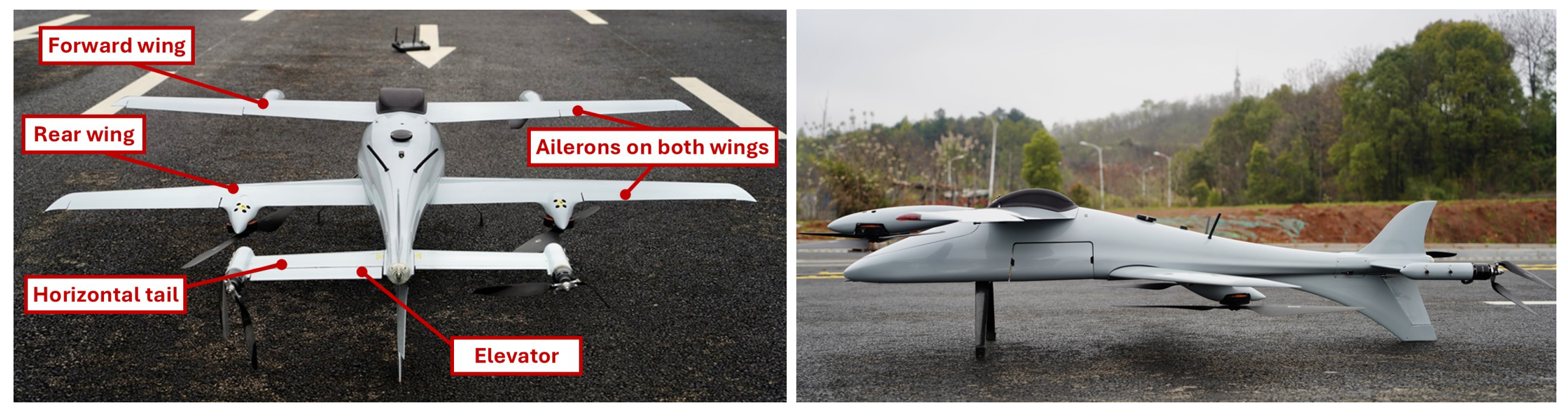
2. Description of the Reference Aircraft: The Dragonfly DS-1

The Dragonfly DS-1, developed and manufactured by Overspace Aviation Srl [18], is employed in this study as a reference fixed-wing VTOL drone for validating the modeling procedure proposed in this work. This aircraft serves as an excellent case study because it features an innovative three-surface configuration that combines tandem wings, a horizontal stabilizer, and a downward-facing vertical stabilizer. Each wing is equipped with dedicated ailerons to control roll movements, while the horizontal stabilizer integrates an elevator. Finally, the rudder is integrated into the downward-facing vertical stabilizer. The aircraft is equipped with six rotors in total, which enable both vertical take-off and landing and horizontal flight in airplane mode. Four rotors are dedicated to quadcopter operations and are mounted on the structural supports extending from the semi-wings. The propulsion for forward horizontal flight is provided by two rear-mounted rotors. Figure 1 shows the upper and side views of the reference aircraft. The main dimensions and specifications of the aircraft are reported in

Table 1. Relevant technical specifications of the Dragonfly DS-1.

Specification	Value
Dimensions (L × W × H)	1984 × 2000 × 481 mm
Flight Mass	22.5 kg
Flight Altitude	120 m
Standard Cruise Speed	27 m/s
Max Speed	45 m/s
Rear Motor	T-Motor AT4130 Long Shaft [19]
Propeller	APC 16 × 8

.

Even though the Dragonfly DS-1 is designed to offer improved performance during hover and vertical flight, in this study, the analysis is focused exclusively on the aircraft flight mechanics of fixed-wing flight mode, excluding the transition and VTOL phases.

In addition to the main airplane characteristics, Overspace Aviation Srl also provided the total mass, the position of the center of gravity, and a detailed CAD model from which it was possible to extract all the geometrical data.

3. Development of Flight Mechanics Model Using Semi-Empirical Method

The purpose of this section is to define the methodology used to develop the flight mechanics model of the Dragonfly DS-1. To do so, the USAF Digital DATCOM software [12,20] was employed to estimate the aerodynamic properties of the reference aircraft.

The Digital DATCOM was originally developed to support preliminary aircraft design, allowing users to compute the stability and control derivatives, aerodynamic coefficients, and trim characteristics for traditional configurations, i.e., isolated lifting surfaces, coupled wing–fuselage, coupled wing–fuselage–horizontal tail, or coupled canard–wing–fuselage systems. Consequently, it does not support non-standard designs like three-surface configurations or complex VTOL geometries.

That being said, DATCOM offers a computationally efficient framework that can be exploited for the case at hand. Specifically, the proposed procedure for defining the aerodynamic model is based on four sequential DATCOM analyses, each aimed at providing part of the whole model. Finally, the overall model was constructed by combining all the results of single DATCOM runs.

3.1. Definition of Aircraft Model and Flight Regimes of Interest

A detailed description of the Dragonfly DS-1 geometry was derived from the aircraft CAD model, especially for the fuselage, which features a different shape than the usual “tube” design.

Table 2. Reference parameters employed for aerodynamic coefficient normalization.

Parameter	Symbol	Value
Reference area	$S_{\mathrm{ref}}$	0.77 m2
Longitudinal reference length	$c_{\mathrm{ref}}$	0.209 m
Lateral reference length	$b_{\mathrm{ref}}$	2.0 m

reports some of the main geometrical characteristics of the reference airplane, which were also employed to extract the dimensionless aerodynamic coefficient. The center of gravity and total mass were accurately measured by the manufacturer.

The aerodynamic characterization in DATCOM is based on two primary methods for defining airfoil sections: using standard NACA designations or explicitly providing the coordinates of the profiles. While NACA profile aerodynamics are already part of the DATCOM database, for generic (non-NACA) airfoils, additional details need to be specified, including the coordinates of the upper and lower surfaces, as well as the maximum camber of the airfoils themselves. The wings of the reference airplane feature the Wortmann FX 63-137 airfoil, whose characteristics were taken from an open database [21], whereas the horizontal and vertical tails are both based on the NACA 0010.

In DATCOM, each control surface should be analyzed separately to extract its specific impact, which was later integrated into the overall aerodynamic model. For the analyzed airplane, this aspect is of particular interest because each wing features a set of independent ailerons.

The process of constructing the flight mechanics model of the Dragonfly DS-1 involved performing a series of sequential analyses in Digital DATCOM to systematically quantify the aerodynamic coefficients, stability, and control derivatives. First, it is important to consider some limitations of the DATCOM analyses for these innovative configurations. In particular, three-surface configurations are not included in the DATCOM database. To address this limitation, the aerodynamic model was constructed by decomposing the aircraft into subsystems for which the aerodynamic contributions were evaluated separately and, afterward, suitably combined. Moreover, the tail features a complex layout that does not fit within the standard input framework of the software. As a result, an equivalent tail geometry was considered, preserving its fundamental aerodynamic characteristics while ensuring compatibility with DATCOM inputs. Additionally, the nacelles and the ground supports are not explicitly modeled. For these subcomponents, a dedicated empirical model was considered.

The following list provides a detailed breakdown of the sequential analyses performed, explaining how each component was modeled and how its aerodynamic characteristics were evaluated and combined in the overall model:

• Analysis 1: This analysis considers the fuselage, both the front and rear wings, and the ailerons located on the front wing. The geometry of these wings is the same as that of the physical aircraft. When two lifting surfaces are inputted, DATCOM allows the user to include ailerons on the surface with the lowest span. In the analyzed case, the wings have the same span and, consequently, the rear wing span is artificially reduced by $1 \mathrm{cm}$. This analysis provides the modeling of the foremost part of the airplane, including the presence of the ailerons located on the front wing.
• Analysis 2: The considered model is formally equal to that analyzed in the first step, but in this case, the ailerons are placed on the rear wing. To do so, the front wing span is artificially reduced by $1 \mathrm{cm}$ so as to trigger the canard configuration in DATCOM.
• Analysis 3: This analysis considers both the physical horizontal and vertical tails along with an artificial wing described through the aerodynamic coefficients obtained in “Analysis 1”. The artificial wing, as defined, is geometrically identical to the real rear wing but incorporates the combined effect of the rear and front wings and their mutual interference. This approach is made possible by the fact that DATCOM allows one to directly input the aerodynamic coefficients of a lifting body as if they were experimental data. Clearly, even if the artificial wing is described by the aerodynamic coefficients of the combined tandem wings, its shape, for example, in terms of taper and sweep angle, may have an impact on the overall aerodynamic characteristics. These characteristics can be treated as tuning parameters selected based on the problem at hand. The physical horizontal tail model also incorporates the elevator degrees of freedom. Finally, the vertical tail and the vertical fin of a suitable geometry approximating the real one are included in the analysis.
• Analysis 4: This last analysis considers the isolated fin equipped with the rudder and is only included to evaluate the control derivative with respect to rudder deflection.

Figure 2 shows renders of the DATCOM runs associated with the first three analyses.

Once all the DATCOM analyses were performed, the aerodynamic model could be constructed. In particular, the steady aerodynamic coefficients $C_L$ and $C_D$ and the related variations as functions of the angle of attack $\alpha$ and the elevator deflection ${\delta }_E$ were directly extracted from the results of “Analysis 3”, providing a comprehensive representation of the aerodynamic characteristics of the aircraft. The lateral-directional derivatives, including the side-force coefficient derivative with respect to the sideslip angle ($C_{Y\beta }$), as well as the yawing and rolling moment coefficient derivatives ($C_{\mathcal{N}\beta }$ and $C_{\mathcal{L}\beta }$), were extracted from the same analysis. The rolling and yawing moments induced by the front wing aileron and rear wing aileron deflections were extracted from “Analysis 1” and “Analysis 3”, respectively.

It is noteworthy that the current methodology can be adapted to model various configurations. For instance, it can be extended to accommodate an arbitrary number of lifting surfaces by analyzing each one individually in conjunction with an artificial wing that synthesizes the effects of all forward surfaces. Additionally, a box-wing configuration can be achieved by positioning two wings with appropriate sweep and dihedral angles so that their tips meet, forming a continuous lifting surface. Clearly, these extensions are beyond the scope of this work.

3.2. Drag Estimation for Unmodeled Nacelles and Ground Support Structures

Although the approach presented in Section 3 provides a structured methodology for estimating the aerodynamic model, additional empirical corrections are required to account for unmodeled subcomponents, such as the nacelles and the ground supports. Regarding the ground support elements, for simplicity, we assumed that their contribution was negligible due to their small cross-sectional area. More sophisticated modeling based on dedicated corrections would be required. The aerodynamic contribution of the nacelles of the support structure was based on empirical correlations derived from the classical aerodynamics literature [22,23], which provide a treatment for the estimation of both the friction and form drag for elements that have a high length-to-diameter ratio and are aligned to the streamwise flow. The procedure resulted in a limited addition of drag, approximately quantified as 0.001, confirming that the aerodynamic contribution of the nacelles is minimal.

3.3. Final Model

In this section, the aerodynamic trends obtained by combining the four analyses from Section 3.1 are presented. Figure 3 shows, on the right, the variation in the lift coefficient $C_L$ with the angle of attack $\alpha$ for different values of the elevator deflection ${\delta }_E$, and on the left, the aerodynamic polar, showing the relationship between $C_D$ and $C_L$.

Looking at the obtained lift and drag curves, it is possible to derive some preliminary comments. First, the impact of the elevator deflection is limited, although visible, as expected in both the lift curve and the polar. Moreover, the low value of the zero-lift angle of approximately $-8 \mathrm{deg}$ with zero elevator deflection is somewhat unusual but aligns with the expectation given the airfoil used, the Wortmann FX 63-137 airfoil, which features similar characteristics.

4. Sensitivity Analyses and Model Refinement Strategies

In this section, we perform sensitivity analyses to evaluate the impact of some assumptions made in the modeling process (see Section 3), with specific emphasis on the characteristics of the artificial wing in “Analysis 3”.

In the following, the sensitivity of the polar data with respect to the artificial wing position, area, and taper ratio is analyzed.

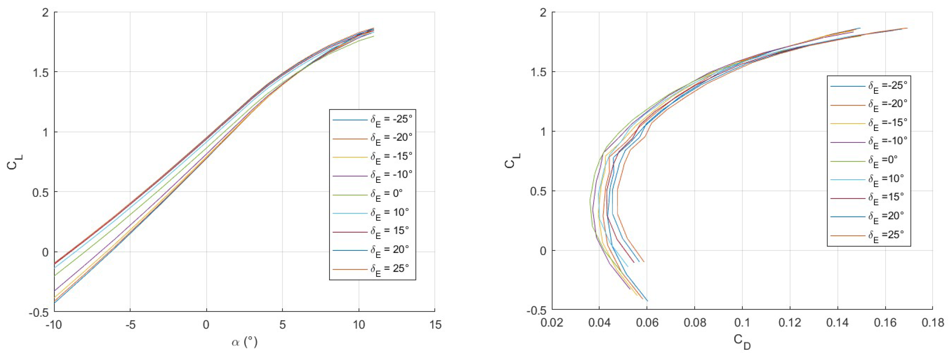
4.1. Variation in Artificial Wing Position

To systematically investigate the effect of the wing position, the artificial lifting surface was progressively displaced both longitudinally and vertically, covering the range between its initial position (corresponding to the secondary wing) and the position of the front wing. The goal of this analysis was to understand how the aerodynamic parameters of the vehicle were affected when the equivalent wing moved toward the forward lifting surface. For simplicity, this analysis was conducted under the assumption that ${\delta }_E=0$ to ensure that the comparisons would not be influenced by control surface deflections.

Figure 4 presents the trends of the computed aerodynamic coefficients. The left plot illustrates the behavior of the lift coefficient $C_L$ as a function of the angle of attack, while the right plot shows the aerodynamic polar. Both plots are parameterized with the artificial wing location, with $x_w$ and $z_w$ being the longitudinal and vertical coordinates of the wing apex. The results presented in the graphs indicate that the lift coefficient and the polar showed limited sensitivity to changes in the longitudinal and vertical positions of the equivalent wing, with variations remaining within a narrow range for the entire angle-of-attack spectrum. For example, at zero angle of attack and for the forwardmost position of the artificial wing, the lift coefficient was only 0.6% higher than that of the original model.

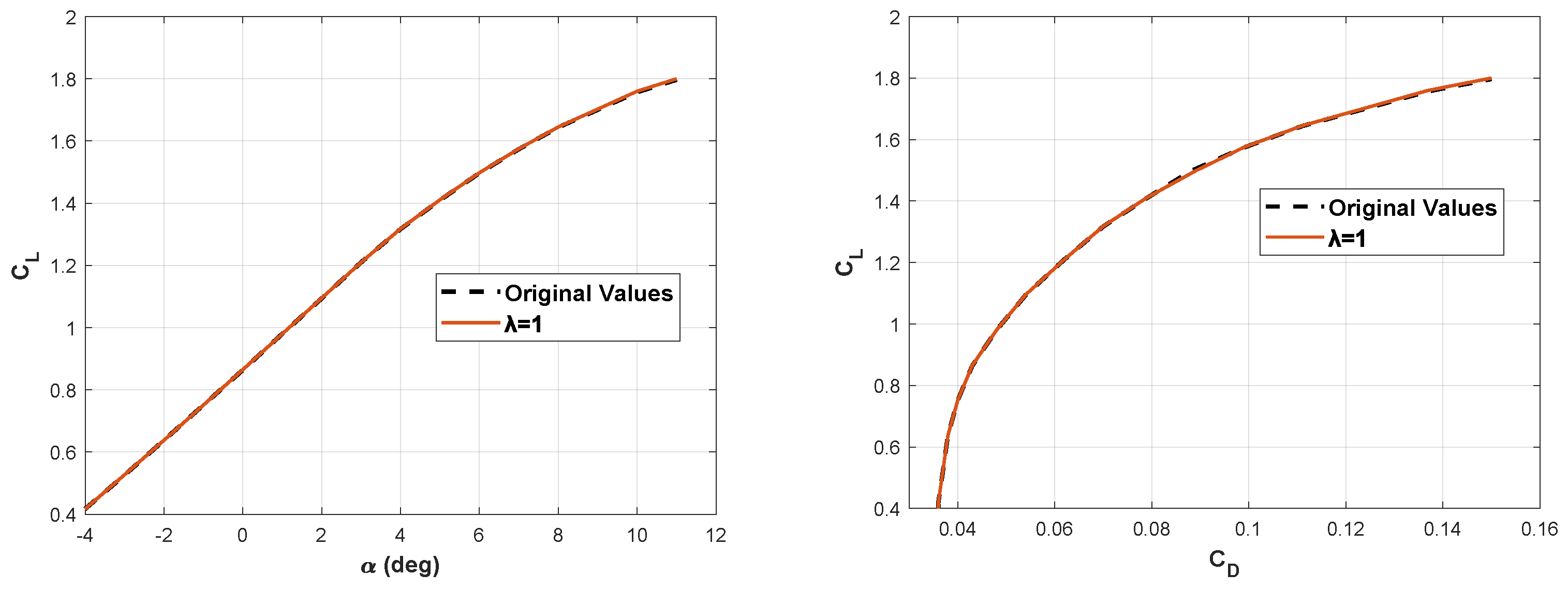
4.2. Variation in Equivalent Wing Area

The second sensitivity analysis focused on the effect of the area of the artificial wing while maintaining a constant wingspan. This was achieved by adjusting the root chord and tip chord of the equivalent wing, effectively altering its aspect ratio and overall aerodynamic properties. The goal of this analysis was to evaluate how changes in the equivalent wing area influenced the aerodynamic coefficients and whether a specific area definition could provide a more representative estimation of the three-surface configuration.

The aerodynamic trends for different equivalent wing areas are presented in Figure 5. The left plot illustrates the variations in the lift coefficient $C_L$, while the right plot shows the aerodynamic polar, $C_L$ vs. $C_D$.

The graphical results confirm that the artificial wing area had a noticeable impact on both the lift and drag coefficients. The lift coefficient $C_L$ showed a clear dependency on the wing area, with larger areas generating higher lift values across all angles of attack. Similarly, the drag coefficient $C_D$ exhibited a slight increase as the wing area grew, as demonstrated by the variation in the aerodynamic polar. For example, at zero angle of attack, the difference between the lift coefficient of the nominal artificial wing and the wing with the largest area was 3.6%.

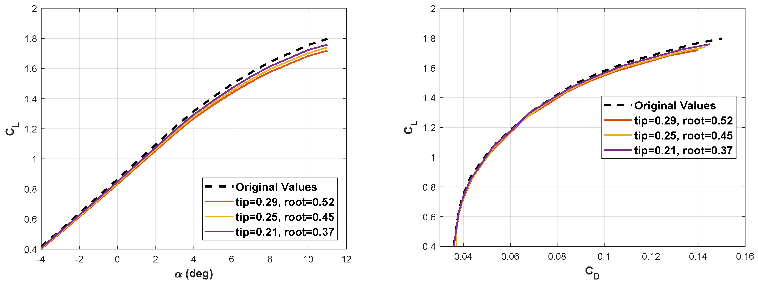
4.3. Variation in Equivalent Wing Taper Ratio

The third analysis investigated the effect of the taper ratio ($\lambda$) of the artificial wing while maintaining a constant reference area. The taper ratio is defined as the ratio between the tip chord ($c_t$) and the root chord ($c_r$).

In the baseline configuration, the equivalent wing has a taper ratio $\lambda$ of approximately $\lambda =0.56$. In this analysis, $\lambda$ was increased up to a value of $\lambda =1$, corresponding to a rectangular wing, while adjusting the chord dimensions accordingly to ensure that the total wing area remained unchanged.

From the trends visualized in Figure 6, it is evident that the taper ratio of the artificial wing had a negligible effect on the aerodynamics. Both the lift coefficient and the polar remained largely unchanged across the analyzed configurations, with minimal differences. At zero angle of attack, the difference in the lift coefficients of the two analyzed cases was equal to 0.1%.

5. Comparative Analysis of CFD Simulations, Experimental Flight Data, and Semi-Empirical Data

Once the flight mechanics model of the Dragonfly DS-1 is derived, it is essential to validate its accuracy by comparing the obtained results against multiple sources. This section focuses on a comparative analysis between the point on the drag polar derived from experimental flight data, the results obtained through the CFD simulations provided by Overspace Aviation, and the curve derived from the semi-empirical model. The goal of this comparison is to validate the consistency and reliability of the different approaches, identifying potential discrepancies and evaluating their impact on the aerodynamic characterization of the reference aircraft. The experimental data provide a direct reference based on real flight conditions, while the CFD simulations offer a high-fidelity numerical prediction of aircraft aerodynamics. First, we describe the procedure used to extract the polar data from the experimental data, and then we present a comparison.

5.1. Methodology for Analyzing Experimental Flight Data

This section outlines the methodology used to analyze the flight logs and derive the relevant aerodynamic parameters for the Dragonfly DS-1. The process includes identifying the flight data sources, applying filtering techniques to eliminate inconsistencies, and processing the data to ensure accurate comparisons with numerical predictions.

The experimental data analyzed in this study originated from a series of flight test campaigns conducted by Overspace Aviation, which were not specifically designed to support modeling and comparison activities.

The logs of each of these flights contain detailed telemetry and sensor recordings from the onboard avionics system. The data were collected using the ArduPilot autopilot system [24], which provides a wide set of measurements, including the following:

• Angular rates, including the roll rate p, pitch rate q, and yaw rate r.
• Linear accelerations along the body-frame axes $a_x$, $a_y$, and $a_z$.
• Speeds extracted from the GPS, including the ground speed (SpD) and the vertical speed ($V_{\mathrm{Z}}$).
• Attitude angles, including the roll ($\varphi$), pitch ($\theta$), and yaw ($\psi$).
• Wind estimation components, including the northward and eastward wind velocities ($V_{\mathrm{WN}}$ and $V_{\mathrm{WE}}$).
• Throttle percentage (Thr), which is the fraction of the maximum available thrust being commanded by the autopilot.

The extracted flight data underwent a structured filtering and processing procedure to identify flight conditions that were as close as possible to uniform rectilinear flight. Given the natural variability of real-world flight conditions, the analysis was designed to select flight segments where variations in speed, attitude, and acceleration were minimized, ensuring that the extracted data were representative of a close-to-steady-state aerodynamic behavior.

To efficiently analyze the data, the following processing steps were implemented in MATLAB R2023a:

• Windowing: To facilitate statistical analysis, the dataset was divided into non-overlapping windows of 10 samples, 0.1 s for each sample. This approach enabled a local statistical evaluation of flight conditions, reducing the effect of transient fluctuations while preserving steady-state behavior.
• Statistical feature extraction: For each flight parameter within a time window, the mean value, the variance, and the maximum and minimum values were computed.
• Selection criteria: The goal of this step was to identify time windows that corresponded as much as possible to straight and level flight, where aerodynamic forces and moments could be reliably analyzed. The selection criteria included the following:
  • Angular rate: To ensure that the UAV was flying as close as possible to uniform rectilinear motion, both the mean values and the variances of the roll rate p, pitch rate q, and yaw rate r were constrained within predefined tolerances, chosen here as $0.1 \mathrm{deg}/\mathrm{s}$ for the mean values and $0.1 {\mathrm{deg}}^2/{\mathrm{s}}^2$ for the rate variances. By enforcing these dual constraints, only flight segments where the UAV maintained stable angular velocities with negligible oscillations were selected, reducing the influence of external disturbances and ensuring a reliable aerodynamic dataset.
  • Linear accelerations: To ensure that the UAV was in near-equilibrium conditions during level flight, the mean values of the accelerations along the body axes were constrained within predefined limits, chosen here as

    $$\begin{array}{cc}\hfill |\overline{a_x}|& <0.3 {\mathrm{m}/\mathrm{s}}^2(\mathrm{small}\mathrm{longitudinal}\mathrm{acceleration})\hfill \\ \hfill |\overline{a_y}|& <0.3 {\mathrm{m}/\mathrm{s}}^2(\mathrm{small}\mathrm{lateral}\mathrm{acceleration})\hfill \\ \hfill |\overline{a_z}+9.81|& <0.2 {\mathrm{m}/\mathrm{s}}^2(\mathrm{consistent}\mathrm{vertical}\mathrm{acceleration})\hfill \end{array}$$

    (1)
    Additionally, the variances of the three accelerations were also constrained to be less than 0.2 ${\mathrm{m}}^2/{\mathrm{s}}^4$. The combination of these constraints ensured that the aircraft did not experience significant dynamic effects and that the extracted flight segments represented steady conditions suitable for quantifying the lift and drag coefficients.
  • Stability of airspeed: To ensure that the aircraft was in a reasonably uniform flight condition, the variance of the specific airspeed (SpD) was constrained to be lower than $0.05 {\mathrm{m}}^2/{\mathrm{s}}^2$.
  • Ground course stability: To ensure that the aircraft maintained a consistent heading, the variance of the heading angle was also constrained to be lower than a threshold of $0.05 {\mathrm{deg}}^2$.
• Finalization of the process: The selected time windows were extracted and stored for aerodynamic evaluation.

From the measurements within the selected time windows, it was possible to compute the discrete points of the aerodynamic force coefficients, specifically the drag coefficient $C_D$ and the lift coefficient $C_L$, by combining onboard sensor data with an external propulsion model. However, direct calculation of these coefficients requires knowledge of the angle of attack $\alpha$, which was not explicitly measured in the available flight logs. Therefore, an additional methodology needed to be developed to estimate $\alpha$ from the recorded telemetry data. This process involved analyzing the velocity components and aircraft orientation to infer the effective angle of incidence during steady flight conditions. Establishing a structured procedure for determining $C_D$, $C_L$, and $\alpha$ from flight data is crucial for validating aerodynamic models and assessing an aircraft’s performance in real operational conditions [25,26].

The flight data logs provide velocity components in the north–east–down (NED) reference frame. However, aerodynamic analyses require these velocity components to be expressed in the body frame. This transformation is achieved using the standard rotation matrix from the north–east–down frame N to the body frame B

$${\mathbf{R}}_{N\to B}=\left[\begin{array}{ccc}cos\psi cos\theta & cos\psi sin\theta sin\varphi -sin\psi cos\varphi & cos\psi sin\theta cos\varphi +sin\psi sin\varphi \\ sin\psi cos\theta & sin\psi sin\theta sin\varphi +cos\psi cos\varphi & sin\psi sin\theta cos\varphi +cos\psi sin\varphi \\ -sin\theta & cos\theta sin\varphi & cos\theta cos\varphi \end{array}\right],$$

(2)

where $\varphi$, $\theta$, and $\psi$ are the Euler angles of sequence 3–2–1, namely the roll, pitch, and heading angles.

The velocity of the aircraft relative to the surrounding air, denoted as ${\mathbf{V}}_{\mathrm{AS}}$, is obtained by subtracting the wind velocity ${\mathbf{V}}_w$ from the ground speed ${\mathbf{V}}_{\mathrm{N}}$. The ground velocity vector in NED coordinates is given by

$${\mathbf{V}}_N=\left[\begin{array}{c}\left|\mathbf{V}\right|cos\left(\chi \right)\\ \left|\mathbf{V}\right|sin\left(\chi \right)\\ V_{\mathrm{Z}}\end{array}\right],$$

(3)

where $\left|\mathbf{V}\right|$, $\chi$, and $V_{\mathrm{Z}}$ are the airspeed, the track angle, and the vertical velocity, respectively, which are pieces of information extracted from the GPS signals.

Similarly, the wind velocity in the NED frame is given by

$${\mathbf{V}}_w=\left[\begin{array}{c}{V}_{\mathrm{WN}}\\ V_{\mathrm{WE}}\\ V_{\mathrm{WZ}}\end{array}\right]$$

(4)

where $V_{\mathrm{WN}}$, $V_{\mathrm{WE}}$, and $V_{\mathrm{WZ}}$ are the components along the north, east, and down directions, respectively.

The airspeed vector in NED coordinates is then computed as

$${\mathbf{V}}_{\mathrm{AS}}^N={\mathbf{V}}_N^N-{\mathbf{V}}_w^N$$

(5)

By applying the inverse of the rotation matrix, these velocity components are transformed into the body frame:

$${\mathbf{V}}_{\mathrm{AS}}^B={\mathbf{R}}_{N\to B}^T{\mathbf{V}}_{\mathrm{AS}}.$$

(6)

The longitudinal, lateral, and vertical components of the airspeed vector ${\mathbf{V}}_{\mathrm{AS}}^B$ are denoted as U, V, and W.

The angle of attack $\alpha$, which, as mentioned before, is not directly measured in the flight logs, is computed from the velocity components in the body frame as

$$\alpha =arctan\left({\displaystyle \frac{W}{U}}\right).$$

(7)

Note that the angle of attack estimate may lead to inaccuracies, particularly under high and variable wind conditions. Therefore, conducting flight campaigns on calm days is advisable.

Once the velocity components are known, the aerodynamic forces acting on the aircraft are estimated using Newton’s second law. The forces in the body axes are given by

$$\begin{array}{cc}\hfill F_x& =m{a}_x-T_{eff}\hfill \end{array}$$

(8)

$$\begin{array}{cc}\hfill F_y& =m{a}_y\hfill \end{array}$$

(9)

$$\begin{array}{cc}\hfill F_z& =m{a}_z\hfill \end{array}$$

(10)

where m is the mass of the aircraft; $a_x,a_y,a_z$ are the measured linear accelerations in the body frame; and T is the thrust force. The non-dimensional aerodynamic force coefficients are then computed as

$$\begin{array}{cc}\hfill C_X& ={\displaystyle \frac{m{a}_x-T_{eff}}{\frac{1}{2}\rho U^{2}S}}\hfill \end{array}$$

(11)

$$\begin{array}{cc}\hfill C_Y& ={\displaystyle \frac{m{a}_y}{\frac{1}{2}\rho U^{2}S}}\hfill \end{array}$$

(12)

$$\begin{array}{cc}\hfill C_Z& ={\displaystyle \frac{m{a}_z}{\frac{1}{2}\rho U^{2}S}},\hfill \end{array}$$

(13)

where $\rho$ is the air density and S is the reference wing area.

To obtain the lift and drag coefficients, the aerodynamic force components are projected along the aerodynamic reference frame as

$$\begin{array}{cc}\hfill C_L& =-C_{Z}cos\alpha +C_{X}sin\alpha \hfill \end{array}$$

(14)

$$\begin{array}{cc}\hfill C_D& =-C_{X}cos\alpha -C_{Z}sin\alpha \hfill \end{array}$$

(15)

The propulsion system of the Dragonfly DS-1 in airplane mode consists of two AT4130 Long-Shaft KV230 brushless motors, with power equal to approximately $1.67 \mathrm{kW}$, each equipped with an APC 16*8 propeller. These motors provide the necessary thrust for horizontal flight, with their performance strongly dependent on the rotational speed (RPM), applied torque, and airspeed.

To evaluate the thrust generated in-flight, it is essential to consider the manufacturer’s static test data, which provides measured thrust values at different throttle percentages [19]. However, these data are obtained under static conditions, i.e., at zero forward velocity, and thus require correction to account for in-flight conditions.

The manufacturer’s data include a look-up table reporting the values of some key parameters as functions of different throttle settings $\xi$. In particular, rotational speed ${\omega }_m\left(\xi \right)$, torque ${\tau }_m\left(\xi \right)$, and the fixed-point thrust $T_{\mathrm{FP}}\left(\xi \right)$ are all available.

To estimate the effective thrust $T_{\mathrm{eff}}$ at a specific velocity and for a specific throttle level, one can use the following procedure. First, one may compute the mechanical power $P_m$ specific to the flight condition as

$$P_m={\mathsf{\Omega }}_m\left(\widehat{\xi }\right){\tau }_m\left(\widehat{\xi }\right)$$

(16)

where $\widehat{\xi }$ is the throttle level measured in the specific flight test. Clearly, evaluating the rotational speed and torque exerted during the test for a specific throttle level requires interpolating the manufacturer’s data using a suitable scheme, chosen here as the straightforward linear scheme.

The actual thrust $T_{\mathbf{eff}}$ can now be computed using the value of the aircraft speed as

$$T_{\mathrm{eff}}=max\left({\displaystyle \frac{P_m}{\left|\mathbf{V}\right|}},T_{\mathrm{FP}}\left(\widehat{\xi }\right)\right).$$

(17)

Given the values of the thrust in a specific segment of a trimmed condition, the lift and drag coefficient estimates can be computed using Equations (8) and (11). The resulting polar can be compared to the CFD simulations and semi-empirical method.

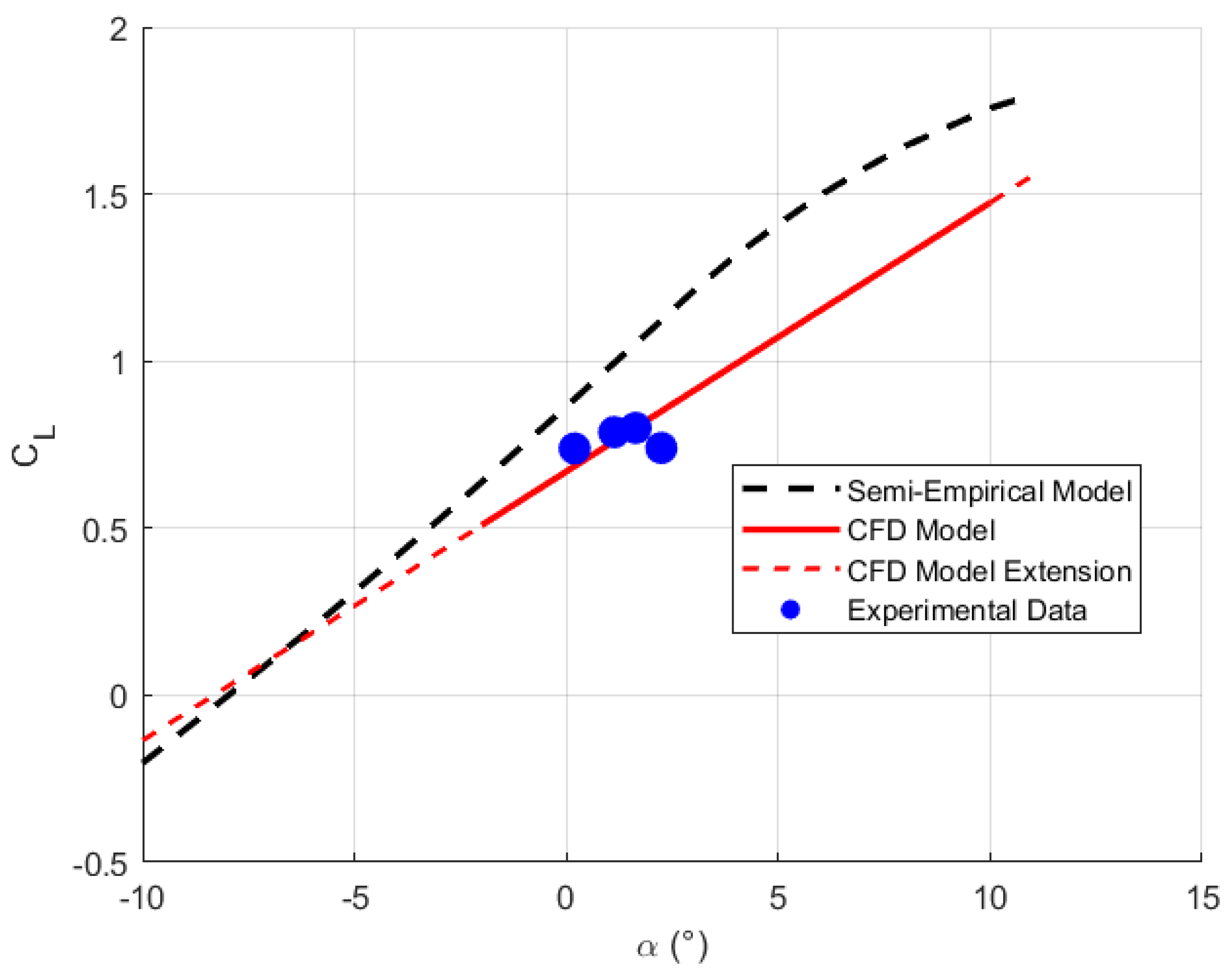
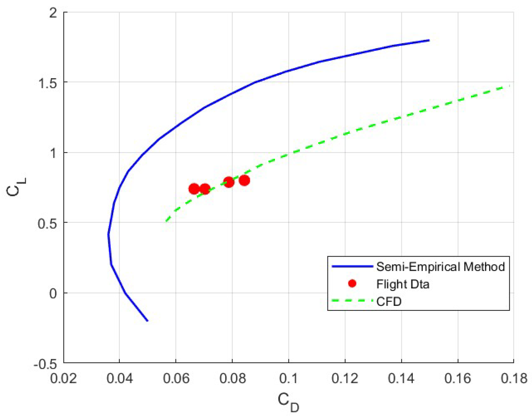
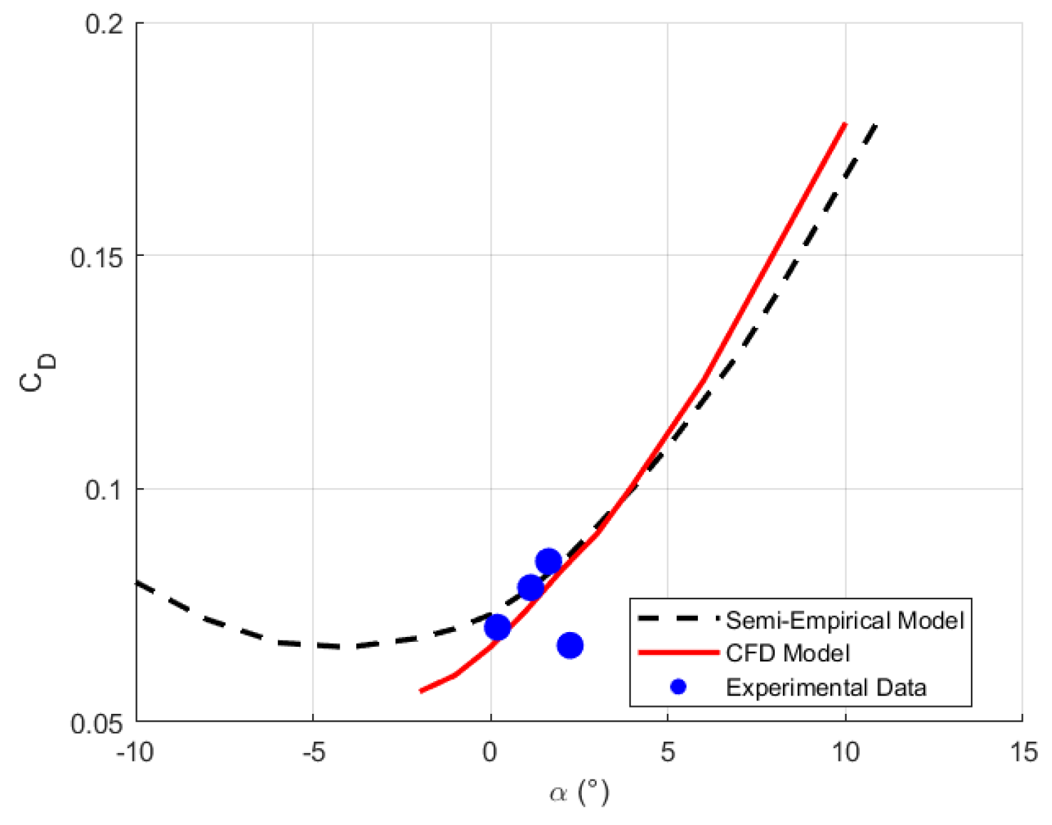
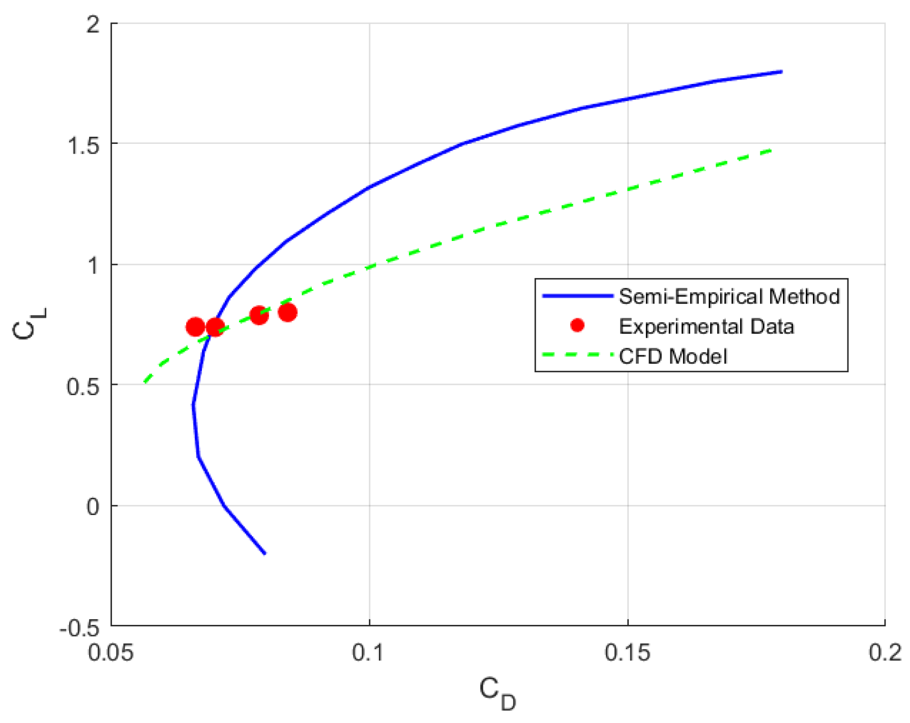
5.2. Comparison of the Drag Polar Between the Experimental Flight Data, CFD Simulations, and Semi-Empirical Method

In this section, a comparative analysis is conducted between the aerodynamic results obtained from the semi-empirical method, computational fluid dynamics simulations, and experimental flight data. The objective is to evaluate the accuracy and reliability of the semi-empirical approach in predicting the drag polar of the Dragonfly DS-1 by benchmarking it against high-fidelity numerical simulations and real-world measurements.

The CFD simulation results, used here for comparison, were obtained using ANSYS Fluent R19.2 [27]. The computational model used for the analysis included the main wings, tailplane, fuselage, and propulsion-supporting structures. To reduce the computational burden, only a symmetric half-configuration and symmetric flight conditions were studied. The CFD computations considered compressible flow, and the flow field was computed by solving the Unsteady Reynolds-Averaged Navier–Stokes (URANS) equations coupled with the SST k-$\omega$ turbulence model. Additionally, the propellers for horizontal flight were set in rotation to capture their aerodynamic influence. The computational domain was discretized using an unstructured mesh with localized refinements applied in critical regions, such as the leading edges of the wings, the fuselage nose, and areas surrounding the control surfaces. It was expected that the CFD simulations would accurately represent the flow separation phenomena and wake structures. The aircraft was simulated in a freestream environment, without ground effects. Since the motor support structures were included in the simulation environment, their additional drag and the local airflow distribution and pressure variations were also captured.

It is important to note that the described CFD process necessitated a dedicated analysis to generate an appropriate mesh and ensure converged results. Besides being time-consuming, the process is also sensitive to specific aircraft geometry details. In contrast, the proposed approach operates on standard hardware within seconds, requires a minimal set of inputs, and is straightforward to implement, visualize, and verify.

To fully assess the validity of the semi-empirical approach, three key aerodynamic characteristics were analyzed: the lift coefficient as a function of the angle of attack ($C_L$ vs. $\alpha$); the drag coefficient as a function of the angle of attack ($C_D$ vs. $\alpha$), highlighting differences in drag estimates among the methods; and the aerodynamic polar ($C_L$ vs. $C_D$), which provides an overall assessment of aerodynamic efficiency by comparing lift-to-drag characteristics across the three methods.

To assess the accuracy of the lift predictions, the results obtained from the semi-empirical method, CFD simulations, and experimental flight data are compared in Figure 7.

The results presented in Figure 7 show noticeable differences between the three approaches. The semi-empirical method exhibits a nearly linear increase in $C_L$ with $\alpha$, followed by a gradual reduction in the slope as the angle of attack increases. This behavior aligns with classical aerodynamic theory but may overestimate the lift contribution due to the simplifications inherent in the equivalent wing approach. The CFD simulations exhibit a linear trend with a lower lift-curve slope compared to the semi-empirical method, suggesting that the numerical approach predicted a reduced lift response, likely due to more realistic modeling of viscous effects and three-dimensional flow interactions. The experimental data points are clustered around small angles of attack, in which the vehicle typically operates in steady flight. This is not optimal from a validation standpoint, as one would require a wider angle-of-attack range, but the available data are still adequate for the preliminary investigation performed in the present work. The semi-empirical method tends to provide optimistic estimations of the lift characteristics, likely due to its simplified representation of the equivalent wing. The experimental results indicate that the actual aerodynamic performance of the Dragonfly DS-1 is similar to that of theoretical models, reinforcing the need for empirical corrections to improve predictive capabilities using semi-empirical methods.

Table 3. Comparison between CFD and semi-empirical values.

Parameter	CFD Value	Semi-Empirical Value	Percentage Error
${\alpha }_0$ (°)	$-8.{32}^{\circ }$	$-7.{97}^{\circ }$	4.2%
$C_{L_{\alpha }}$	$0.08$	$0.1$	24.8%

presents a comparison between the CFD estimates and the proposed approach in terms of the zero-lift angle ${\alpha }_0$ and the lift-curve slope $C_{L_{\alpha }}$. As is clear from the obtained results, the estimates of ${\alpha }_0$ are satisfactory, while the estimates of $C_{L_{\alpha }}$ are acceptable for preliminary design phases.

Figure 8 presents a comparison between the semi-empirical method, CFD simulations, and experimental flight data.

The trends observed in Figure 8 indicate that all three approaches followed similar overall trends, with $C_D$ increasing as $\alpha$ grew. However, a noticeable offset was present between the curves. The semi-empirical model predicted lower drag values over the entire angle-of-attack range, which could be attributed to its simplified approach in representing the equivalent wing aerodynamics. The CFD simulations, on the other hand, estimated higher drag coefficients, particularly at larger angles of attack, where viscous effects and flow separation became more significant. The experimental data points fell between the two numerical models but were consistently higher than the semi-empirical predictions. This suggests that additional drag sources, such as interference effects from different components of the aircraft, structural contributions, and unmodeled aerodynamic interactions, influence the performance of real aircraft. The presence of an offset between the experimental and theoretical curves indicates that the semi-empirical method underestimated the total aerodynamic drag, which may necessitate empirical corrections to improve its predictive capabilities.

The consistency in the shape of the curves across all three methods confirms that the overall trend of the drag was correctly captured by the models. However, the discrepancy in magnitude highlights the importance of accounting for secondary aerodynamic effects that are not fully incorporated in the simplified approach. This offset suggests that refining the semi-empirical model by introducing a correction factor could improve agreement with experimental results.

It can also be observed that there is an experimental point outside the drag trend with the angle of attack. The presence of this outlier may be due to an inconsistent estimation of the angle of attack as a result of an erroneous vertical wind component indication (see Equation (5)). In fact, the wind speed sensing device is not co-located with the airplane body and, consequently, there may be a bias between the measured quantity and the actual value experienced.

Figure 9, which illustrates the comparison between the semi-empirical method, the CFD simulations, and the experimental flight data, highlights the presence of a significant offset between the semi-empirical method and the CFD simulations. This suggests that the simplified assumptions in the semi-empirical formulation led to an underestimation of the parasite drag. The experimental data, representing the real aerodynamic behavior of the aircraft, fell between the two numerical methods but were closer to the CFD predictions. While the general shapes of the curves were consistent across all methods, the differences in magnitude highlight the need to refine the semi-empirical model.

Beyond the adopted simplifications, the DATCOM-based semi-empirical approach inherently carries a margin of error due to its empirical nature. The method relies on pre-established aerodynamic correlations and simplified aerodynamic assumptions that may not fully capture the specific characteristics of the Dragonfly DS-1 configuration. However, given the poor estimation of the parasite drag, introducing a constant correction factor on the drag could improve the predictions and lead to better agreement with experimental observations.

To better align the model with expected behavior, an offset in the drag coefficient, $\Delta C_D=0.03$, was introduced. This adjustment improved the progression of the curve, bringing it closer to the anticipated outcome. Figure 10 and Figure 11 present a final comparison incorporating the constant parasite drag $\Delta C_D$ into the semi-empirical model. The agreement is enhanced, but the calibrated additive parasite drag warrants further investigation in future work to better understand the source of such a significant discrepancy. However, if the goal is to explore minor optimizations of the reference Dragonfly DS-1 configuration, it is reasonable to assume that the constant additive parasite drag will remain unchanged for small geometric modifications.

Although the methodology, including the additional parasite drag, achieved acceptable agreement, it can certainly be improved to achieve closer alignment with the reference data. For example, a combination of multiple semi-empirical methods could be employed, or a dedicated model for upwash and downwash [28] could be implemented to provide more reliable and computationally efficient aerodynamic predictions.

6. Conclusions

This work aimed to develop and validate a structured methodology for modeling the aerodynamic behavior of a three-surface-configuration UAV using semi-empirical methods. Given the unconventional nature of the selected reference aircraft, the Dragonfly DS-1, standard empirical methods such as the Digital DATCOM, originally developed for conventional aircraft geometries, could not be directly applied. To address this limitation, a sequential analysis framework was implemented, decomposing the aerodynamic contributions of the different lifting surfaces and integrating them into a unified aerodynamic representation of the vehicle. This approach enabled structured and computationally efficient estimates of the aerodynamic coefficients, allowing the use of empirical methods in a configuration in which they are not inherently applicable. A sensitivity analysis was also conducted to assess the impact of some geometrical parameters on the aerodynamic predictions.

From the analyses performed in this work, the following conclusions can be derived:

• The CFD simulations based on the URANS methodology provided lift-curve and polar data that aligned closely with the experimental measurements.
• The zero-lift angle was well predicted by the semi-empirical model.
• The agreement between the CFD simulations and the proposed semi-empirical method in terms of the lift slope was insufficient for preliminary investigation and design application, accounting for an error of about 20%. In general, additional improvements to the methodology should be investigated to reduce this error, allowing for routine use of this procedure.
• The comparative validation against the CFD simulations and experimental flight data revealed systematic discrepancies. The most notable difference between the semi-empirical method and the CFD simulations was the offset in the estimation of the drag, where the semi-empirical method consistently underpredicted $C_D$ across the entire angle-of-attack range. Despite these limitations, the overall trends in the aerodynamic polar were correctly captured, indicating that the sequential analysis framework provides a reasonable first-order approximation.

The findings of this work highlight both the strengths and the inherent limitations of applying semi-empirical methods to three-surface configurations. One of the key advantages of the approach developed in this work is its computational efficiency, making it a valuable tool for preliminary design and performance estimation. However, the observed discrepancies indicate that additional improvements in the methodology are required before the approach can be routinely adopted.

Future work should focus on refining the methodology so as to bridge the gap between simplified aerodynamic modeling and high-fidelity simulations. Several potential improvements can be explored. First, one could try using a suitable combination of different semi-empirical methodologies and a dedicated model for upwash/downwash estimation [28], as opposed to the current approach that relies solely on DATCOM. Additionally, one could even use first-principles modeling based on formulation—less sophisticated than CFD—such as vortex-lattice methods, which may offer a better compromise between accuracy and computational burden. Last but not least, expanding the experimentation dataset through a dedicated campaign would be beneficial for the comparative analysis and for providing a more comprehensive understanding of the capabilities and limitations of the proposed modeling approach.

All the aforementioned activities are currently under investigation.

References

1. xflr5. Available online: http://www.xflr5.tech/xflr5.htm (accessed on 10 April 2024).
2. Aviant. Autonomous Drone Delivery. 2024. Available online: https://www.aviant.no (accessed on 27 May 2024).
3. Wing Aviation LLC. Wing—Drone Delivery Service. 2024. Available online: https://wing.com (accessed on 10 April 2025).
4. Swoop Aero. 2024. Available online: https://swoop.aero/our-mission/ (accessed on 10 April 2025).
5. German Drones. Advanced VTOL UAV Solutions. 2024. Available online: https://www.germandrones.com/de/ (accessed on 10 April 2025).
6. Varriale, C.; Lombaerts, T.; Looye, G. Direct Lift Control: A review of its principles, merits, current and future implementations. Prog. Aerosp. Sci. 2025, 152, 101073. [Google Scholar] [CrossRef]
7. Cacciola, S.; Riboldi, C.E.; Arnoldi, M. Three-Surface Model with Redundant Longitudinal Control: Modeling, Trim Optimization and Control in a Preliminary Design Perspective. Aerospace 2021, 8, 139. [Google Scholar]
8. Riboldi, C.E.D.; Cacciola, S.; Ceffa, L. Studying and Optimizing the Take-Off Performance of Three-Surface Aircraft. Aerospace 2022, 9, 139. [Google Scholar] [CrossRef]
9. Goetzendorf-Grabowski, T. Flight dynamics of unconventional configurations. Prog. Aerosp. Sci. 2023, 137, 100885. [Google Scholar] [CrossRef]
10. Bravo-Mosquera, P.D.; Catalano, F.M.; Zingg, D.W. Unconventional aircraft for civil aviation: A review of concepts and design methodologies. Prog. Aerosp. Sci. 2022, 131, 100813. [Google Scholar] [CrossRef]
11. Gallman, J.W.; Smith, S.C.; Kroo, I.M. Optimization of joined-wing aircraft. J. Aircr. 1993, 30, 897–905. [Google Scholar] [CrossRef]
12. Williams, J.E.; Vukelich, S.R. The USAF Stability and Control Digital Datcom: Users Manual; Technical report; McDonnell Douglas Astronautics Company: St. Louis, MO, USA, 1979; Updated by Public Domain Aeronautical Software, 1999. [Google Scholar]
13. Goetzendorf-Grabowski, T.; Figat, M. Aerodynamic and stability analysis of personal vehicle in tandem-wing configuration. Proc. Inst. Mech. Eng. Part J. Aerosp. Eng. 2017, 231, 2146–2162. [Google Scholar] [CrossRef]
14. Kaya, T.; Ozgen, S. Aerodynamic Design and Control of Tandem Wing UAV. In Proceedings of the American Institute of Aeronautics and Astronautics Conference, Dallas, TX, USA, 17–21 June 2019. [Google Scholar] [CrossRef]
15. Kostić, I.; Tanović, D.; Kostić, O.; Abubaker, A.A.I.; Simonović, A. Initial development of tandem wing UAV aerodynamic configuration. Aircr. Eng. Aerosp. Technol. 2022, 95, 431–441. [Google Scholar] [CrossRef]
16. Jemitola, P.; Okonkwo, P. An Analysis of Aerodynamic Design Issues of Box-Wing Aircraft. Purdue Univ. J. 2023, 12, 2. [Google Scholar] [CrossRef]
17. Cappelli, L.; Costa, G.; Cipolla, V.; Frediani, A. Aerodynamic Optimization of a Large PrandtlPlane Configuration. Aerotec. Missili Spaz. 2016, 95, 163–175. [Google Scholar] [CrossRef]
18. Overspace Aviation. Advanced VTOL Technology. 2024. Available online: https://www.os-aviation.com (accessed on 10 April 2025).
19. T-Motor. AT4130 Long Shaft Fixed-Wing Motor. 2024. Available online: https://store.tmotor.com/product/at4130-long-shaft-fixed-wing-motor.html (accessed on 10 April 2025).
20. Fink, R.D. USAF Stability and Control Datcom; Afwal-tr-83-3048; Flight Dynamics Laboratories (AFWAL/FIGC), Air Force Wright Aeronautical Laboratories, Wrigth–Patterson Air Force Base: Dayton, OH, USA, 1978. [Google Scholar]
21. Airfoil Tools. Airfoil Data. Available online: http://airfoiltools.com/ (accessed on 9 April 2025).
22. Hoerner, S.F. Fluid-Dynamic Drag; Hoerner Fluid Dynamics: Bakersfield, CA, USA, 1965. [Google Scholar]
23. Roskam, J. Airplane Design Part VI: Preliminary Calculation of Aerodynamic, Thrust and Power Characteristics; DARcorporation: Lawrence, KS, USA, 2001. [Google Scholar]
24. ArduPilot. Open Source Autopilot. 2024. Available online: https://ardupilot.org (accessed on 10 April 2025).
25. Klein, V.; Morelli, E.A. Aircraft System Identification: Theory and Practice; AIAA Education Series: Reston, VA, USA, 2006. [Google Scholar]
26. Cacciola, S.; Bottá, L.; Riboldi, C.E.; Trainelli, L. Identification of the Impact of Blowing on the Aerodynamic Model of an Airplane with Distributed Electric Propulsion. In Proceedings of the 34th ICAS Congress Conference Proceedings, Florence, Italy, 9–13 September 2024. [Google Scholar]
27. ANSYS Fluent. Computational Fluid Dynamics (CFD) Software, ANSYS Inc. 2024. Available online: https://www.ansys.com/products/fluids/ansys-fluent (accessed on 10 April 2025).
28. Corcione, S.; Bonavolontà, G.; De Marco, A.; Nicolosi, F. Downwash modelling for three-lifting-surface aircraft configuration design. Chin. J. Aeronaut. 2023, 36, 161–173. [Google Scholar] [CrossRef]
Figure 1. Raised upper and side views of the Dragonfly DS-1 [18].
Aerospace 12 00515 g001
Figure 2. DATCOM renders of Analyses 1 and 2 (left) and Analysis 3 (right).
Aerospace 12 00515 g002
Figure 3. (Left) Plot: C L vs. α for different δ E . (Right) Plot: Aerodynamic polar ( C D vs. C L ) for different δ E .
Aerospace 12 00515 g003
Figure 4. Aerodynamic data for different equivalent wing positions. x w and z w are the longitudinal and vertical coordinates of the wing apex in m . (Left) Plot: lift coefficient C L as a function of the angle of attack α . (Right) Plot: aerodynamic polar, C L vs. C D . The results are compared with the original semi-empirical model.
Aerospace 12 00515 g004
Figure 5. Aerodynamic data for different equivalent wing areas. (Left) Plot: lift coefficient C L as a function of the angle of attack α . (Right) Plot: aerodynamic polar.
Aerospace 12 00515 g005
Figure 6. Aerodynamic data for different equivalent wing taper ratios. (Left) Plot: lift coefficient C L as a function of the angle of attack α . (Right) Plot: aerodynamic polar.
Aerospace 12 00515 g006
Figure 7. Comparison C L as a function of α between the semi-empirical method, CFD simulations, and experimental flight data.
Aerospace 12 00515 g007
Figure 8. Comparison of C D as a function of α between the semi-empirical method, CFD simulations, and experimental flight data.
Aerospace 12 00515 g008
Figure 9. Comparison of aerodynamic polar ( C L vs. C D ) between the semi-empirical method, CFD simulations, and experimental flight data.
Aerospace 12 00515 g009
Figure 10. Comparison of C D as a function of α between the semi-empirical model (with corrected parasite drag), CFD simulations, and experimental flight data.
Aerospace 12 00515 g010
Figure 11. Comparison of aerodynamic polar ( C L vs. C D ) with corrected C D between the semi-empirical model (with corrected parasite drag), CFD simulations, and experimental flight data.
Aerospace 12 00515 g011