Abstract
To investigate the phenomenon of liquid xenon flashing in a filling pipeline, the two-phase flow in a pipe is calculated and analyzed by using a one-dimensional homogeneous equilibrium model (HEM) and a two-dimensional mixture model. The distribution of xenon two-phase flow parameters along the pipeline is observed by the numerical solution of a one-dimensional HEM and simulation by Fluent. The comparison and analysis of the results of different models show that the one-dimensional HEM can quickly attach the critical mass flux faster than Fluent’s simulation under the given filling conditions, which verifies the rationality and rapidity of the numerical solution in calculating the flash process. The influence of the diameter and length of the pipeline on the flashing process of liquid xenon is analyzed by a one-dimensional theoretical model. The results show that the geometric parameters of the pipeline have a great impact on the mass flow rate and the position of the initial phase transition point, but have little effect on the void fraction at the outlet. An increase in pipe diameter and pipeline length delays the onset of phase transition. Compared with liquid oxygen and liquid nitrogen, liquid xenon is more likely to undergo a phase transition. The phase change kinetics of oxygen and nitrogen are roughly 70% as fast as those of xenon.
1. Introduction
Electric propulsion is an advanced space propulsion technology, and xenon is one of its commonly used working fluids. With the development of aerospace low-temperature technology, the low-temperature liquid storage and refueling of liquid xenon—with its high storage density and low pressure—has been made more promising. Liquid propellants may undergo phase transitions in pipelines due to pressure reduction or heating, resulting in gas-liquid two-phase flow, which is not conducive to the continuous filling process. Analyzing the two-phase flow characteristics of liquid xenon in pipelines is a key issue in designing a liquid xenon filling system.
The phenomenon of heat and mass transfer in liquids that undergo phase transition due to pressure reduction and the growth rate of bubbles being affected by the interfacial heat flow rate is called flash evaporation [1]. Lin et al. [2] used a one-dimensional homogeneous flow model to calculate the flash flow of refrigerant R12 in a capillary tube. Yin et al. [3] used a one-dimensional two-phase flow model for flash flow inside a nozzle, while the phase transition model adopted a homogeneous relaxation model, taking into account the nonequilibrium state of the gas. Liang et al. [4] numerically calculated and analyzed the flash flow of refrigerants R12 and R134a in pipelines based on a one-dimensional drift flow model, and the friction coefficient of the two-phase flow section was obtained using the Churchill relationship. The variation in dryness along the capillary is nonlinear, growing rapidly during the initial stage of vaporization and increasing sharply near the outlet. The void fraction rises abruptly after the flash point and approaches 1.0 near the exit. Seixlack et al. [5] used a two-fluid model to calculate and analyze the flash flow of refrigerants in pipes. The results show that the pressure of refrigerant R134a along the pipe is very close to the saturation pressure, and the temperature and gas–liquid velocity distributions along the pipe are very close, which indicates that the two assumptions of a gas–liquid thermodynamic equilibrium and equal gas–liquid velocity in the homogeneous flow model are reasonable. The two-fluid flow model has an average absolute error of 2.4% in predicting the critical mass flow rate. In recent years, several scholars have attempted to use commercial software to simulate flash flow in refrigerant tubes. Zhu et al. [6] used ANSYS CFX 18.2 to simulate the flash flow of refrigerant R134a in a Laval nozzle. The phase transition model was a dual fluid model, and the simulation results were consistent with the experimental results. Prajapati et al. [7] used Fluent to calculate adiabatic two-phase flow in pipes using the VOF model for two-phase flow and the Lee model for phase transition, with a relaxation factor value of 110. The bubble concentration is higher near the wall until the entire cross-section is filled with a uniform vapor–liquid mixture. Rahul et al. [8] used Fluent to calculate the flash flow inside a tube, the multiphase flow model used the mixture model, and the phase change model used an improved cavitation model. By continuously reducing the outlet pressure, a mass flow outlet pressure curve was drawn to determine the critical flow rate. After the flash point, the effective density and velocity of the fluid change due to variations in the vapor volume fraction, leading to a nonlinear pressure distribution. For subcooled inlet conditions, the model-predicted mass flow rate agrees well with experimental data, with an error within 5%. Luo Meng et al. [9] used the CFD-DPM method under the Eulerian Lagrange framework, used polynomials to fit the gas–liquid physical parameters based on temperature changes, and used Fluent to simulate the gas–liquid two-phase flow field in the flash process. The results show that the model can accurately predict flash spray characteristics. Chauhan et al. [10] used Fluent to calculate the flash flow in geothermal wells using a six equation model as the control equation. The phase change model was in a nonequilibrium state at the gas–liquid interface, and the calculated results were consistent with the experimental results. Li Yafei et al. [11] used the mixture two-phase flow model in Fluent to calculate the flash phenomenon of supercritical carbon dioxide in the rapid expansion process. The model coupled the temperature-driven evaporation condensation model phase change mechanism and the pressure-driven cavitation condensation phase change mechanism. Through UDF, bilinear interpolation was carried out using pressure and temperature to calculate the physical parameters of carbon dioxide, and the accuracy of the model was verified with experimental results in the literature. Andreev et al. [12] proposed a mathematical model for rapid evaluation of flash boiling, which requires minimal actual process parameters to achieve fast yet sufficient assessment of heat and mass transfer processes. Kronenburg et al. [13] developed an extended Eulerian–Lagrangian Spray Atomization (ELSA) model specifically for simulating flash boiling phenomena. The model was validated using cryogenic liquid nitrogen experiments, demonstrating its applicability not only for fuel injection in cryogenic liquid rocket engines but also for other engineering applications involving flash boiling. Zhe Zhang et al. [14] employed the VOF method with customized flash boiling phase-change and nucleation models to numerically investigate static flash boiling processes. Their study revealed the spatiotemporal characteristics of local heat transfer coefficients during flash boiling. The results showed that non-uniform distributions of temperature and pressure fields lead to uneven internal heat transfer in static flash boiling conditions.
At present, there are few reports on the two-phase flow characteristics of liquid xenon. Regarding the two-phase flow that occurs during the transportation of low-temperature propellants in pipes, the influence of external heat on phase change has been studied, such as the precooling of the pipe wall at room temperature [15], and there is little research on the flash evaporation process and flow characteristics inside the pipe. In the field of air conditioning and refrigeration, there is abundant research on the adiabatic flash evaporation of refrigerants in capillaries, which can serve as a reference. This work uses a one-dimensional homogeneous flow model and Fluent simulation to calculate the flashing process of subcooled liquid xenon in pipelines [16]. The effects of the pipeline diameter and length on the flashing process and the flashing characteristics of different working fluids in the refueling pipeline were studied, demonstrating high computational efficiency, revealing xenon’s distinctive propensity for phase transition, providing reference data for liquid xenon in orbit refueling.
2. One-Dimensional Liquid Xenon Pipeline Flash Evaporation Model
Generally, the propellant in the refueling tank is a saturated liquid or a supercooled liquid. The supercooled propellant undergoes flash evaporation in the pipeline to form a two-phase flow, which can be divided into two stages: the single-phase flow section and the two-phase flow section.
In the single-phase flow section, the fluid is an undercooled liquid, considered an incompressible fluid with constant density and constant velocity under steady-state flow conditions. Under microgravity conditions, the influence of gravity on pipeline flow is ignored. Therefore, ignoring the convection and penetration terms of the equation in the single-phase flow section, the pipeline pressure drop is only the frictional pressure drop:
where is the pressure; is the velocity; is the mass flow density, the mass of fluid passing through a unit area per unit time, equal to ; is the Darcy friction coefficient; the subscripts represent the liquid; and is the diameter.
Ignoring the accelerated pressure drop and slightly deforming Formula (1), the mass flow rate in the pipeline is
where represents the mass flow rate, equal to ; represents the cross-sectional area of the pipe. represents the pressure difference between the inlet and outlet of the pipeline, is the density, and is the length of the pipeline. Formula (2) approximates the mass flow rate in the reaction pipeline and can be used to analyze the effects of density, diameter, and pipe length on the mass flow rate.
In the two-phase flow section, as the pressure decreases to the saturated vapor pressure, the liquid xenon undergoes a phase transition, generating steam and forming a gas–liquid two-phase flow in the pipeline. Gas–liquid two-phase flow is considered to be in a thermodynamic equilibrium state, so the two-phase flow section can adopt the homogeneous equilibrium flow (HEM) model. The idea of the homogeneous flow model is to treat two-phase flow as single-phase flow. There are two basic assumptions: the gas-liquid two-phase flow is in thermodynamic equilibrium; that is, the temperature, pressure and chemical potential between the gas and liquid are equal; the velocities between the gas and liquid are equal.
Assuming that the flow is a one-dimensional, steady-state, adiabatic, equal-diameter circular tube, ignoring axial heat conduction, the one-dimensional homogeneous flow equation system is [2]
where is the density of two-phase flow, is the dryness, and is the specific enthalpy of two-phase flow, also known as the static enthalpy, which represents the total enthalpy of two-phase flow. Subscripts and represent liquid and gas, respectively. The common Churchill relationship is used for the friction coefficient [2]. The frictional pressure drop of two-phase flow is calculated based on the average viscosity [2]
where is the viscosity.
According to the homogeneous flow model, the calculation formula for the void fraction [17] is
By slightly modifying Formula (7), the expression for dryness can be obtained
3. Model Solution and Comparison
3.1. Initial Conditions
The filling pipeline is assumed to be an equal diameter circular tube with a length of 2 m, a diameter of 4 mm, and an absolute roughness of 0.002 mm.
In orbital refueling, compression refueling is adopted, assuming that the inlet pressure is constant and that the propellant in the refueling tank is in a supercooled state. The injected tank is considered to continuously exhaust during the refueling process, resulting in a constant outlet pressure. The inlet pressure for filling is 1 MPa, the inlet temperature is 213.61 K, and the outlet pressure is 0.6 MPa.
The saturation pressure corresponding to the liquid xenon inlet is 0.8487 MPa, and the inlet subcooling is 5 K. When the inlet subcooling is 0, the propellant in the supply tank is in a saturated state. Due to flash evaporation, two-phase flow will form in the pipeline, and there is no single-phase flow section in the pipeline. The higher the inlet subcooling is, the longer the single-phase flow section. When the outlet pressure is higher than the saturated vapor pressure corresponding to the inlet temperature, flashing will not occur in the pipeline. This article studies the flow situation in the filling pipeline when the pressure of the injection storage tank is lower than the saturated vapor pressure corresponding to the inlet temperature, so the outlet pressure is set to be slightly lower than the saturated pressure.
3.2. Model Solving Settings
3.2.1. Setting of the One-Dimensional Homogeneous Flow Model
The programming tool used was MATLAB 2016a. During programming, the “shooting method” is used to solve the problem of known pipeline inlet pressure and outlet pressure. Assuming a flow rate, calculate the pressure at the outlet of the pipeline. When the difference between the calculated pressure and the given pressure is small enough, the flow rate is considered to meet the requirements. The pipeline was divided into 2000 cells, each with a length of 1 mm. The calculation can be divided into two parts: single-phase flow and two-phase flow. In the single-phase flow section, the solution can be directly and recursively solved. In the two-phase flow section, the pressure correction method is first used to iteratively calculate the pressure at the next node of the cell, and then the next cell is calculated. The other physical parameters are obtained from REFRPOP 9.0 and made into a numerical table for linear interpolation. The pressure change in the numerical table increases by 0.002 MPa.
3.2.2. Fluent Settings
Fluent has a mesh count of 8393 and uses a quadrilateral mesh. In general, the solver uses pressure-based solvers and steady-state and two-dimensional axisymmetric models, which can reduce computational complexity. The multiphase flow model adopts the mixture model. The mixture model is a simplified multiphase flow model in which the gas and liquid phases have the same pressure and temperature, taking into account the slip velocity between the gas and liquid phases, allowing for mutual infiltration between the phases. In the multiphase flow model, the main phase is the liquid phase, and the secondary phase is the gas phase. The phase transition model uses the Fluent evaporation condensation model, also known as the Lee model. The value of the relaxation factor is selected as 120. The saturation temperature is set as a function of pressure, which is obtained via piecewise linear interpolation. The saturation temperatures under different pressures are shown in Table 1. The turbulence model adopts the realizable model, and the near-wall treatment uses the standard wall function.

Table 1.
Saturated pressure and saturated temperature.
In terms of material properties, the density of the gas phase is calculated based on the R-K (Redlich Kwong) real gas equation. The remaining physical parameters are calculated via two-point linear interpolation. In terms of the boundary conditions, the inlet is a pressure inlet, the estimated turbulence intensity is 3.55%, and the hydraulic diameter is 0.004 m. The outlet adopts a pressure outlet, and the wall surface adopts an adiabatic nonslip boundary condition. The boundary conditions for the inlet and outlet are the same as those used in the homogeneous flow model. In terms of the solving settings, the pressure velocity coupling adopts the SIMPLE format, and the pressure adopts the PRESTO! format. The QUICK format is used for density, momentum, volume fraction, turbulent kinetic energy, turbulent dissipation rate, and energy. Due to the difficulty in convergence and divergence of multiphase flow calculations accompanied by heat and mass transfer, a first-order upwind scheme can be used in the calculation process, with the physical parameters set to constant values. The settings can be adjusted after the flow field stabilizes.
3.3. Numerical Results Comparison
3.3.1. Comparison of the Numerical Calculation Results with the Fluent Simulation Results
Compared to one-dimensional models, Fluent can obtain more information and provide the radial distribution of flow parameters. The mass flow rates of the pipeline under different relaxation factors are shown in Table 2. By adjusting the relaxation factor, the mass flow rate in the pipeline is similar, and the error is controlled within 0.5%. The mass flow rates calculated by the Fluent and one-dimensional homogeneous flow models are shown in Table 3. The flow parameter distributions calculated by Fluent and the one-dimensional homogeneous flow model are shown in Figure 1.
Table 2.
Mass fluxes under variable relaxation parameters.
Table 3.
Error of mass flux.
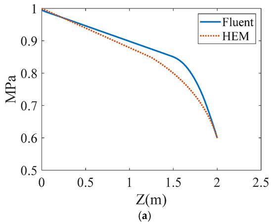
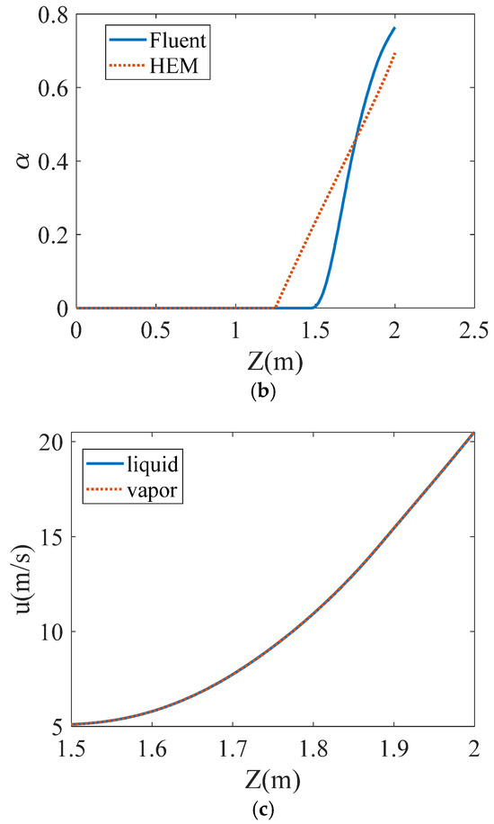
Figure 1.
Comparisons of model predictions with Fluent simulations. (a) Pressure distribution; (b) gas volume fraction distribution; (c) velocity distribution.
The calculation results of Fluent depend on the selection of relaxation factors in the phase transition model. The relaxation factor, also known as the mass transfer intensity coefficient, can be used to regulate the mass transfer rate. When the relaxation factor is too small, the mass transfer rate between gas and liquid is slow, and almost no phase transition occurs in the pipeline. When the relaxation factor is too large, the phase transition becomes severe. The relaxation factor is used to maintain the interface temperature near the saturation temperature. The selection range of relaxation factor values is wide, ranging from 0.01 to hundreds or even thousands. The selection of relaxation factor values is related to the geometric structure, flow conditions, mesh size, and time step selection [18,19]. The selection of relaxation factors in the literature is generally based on experimental control or direct reference to previous work. At present, there have been no two-phase xenon flow experiments in pipelines, nor have there been numerical calculations related to xenon two-phase flow. Therefore, this article combines the literature on refrigerant flash evaporation and compares the mass flow rate calculated by adjusting the relaxation factor with the one-dimensional homogeneous flow model. Finally, the value of the relaxation factor is selected as 120. Through Figure 1a,b, it can be found that the position where the phase transition point occurs in the Fluent calculation is later than that calculated by the one-dimensional homogeneous flow model. In the two-phase flow section, the phase transition process is more intense than that in the one-dimensional homogeneous flow section. By calculating the slip velocity between the gas and liquid shown in Figure 1c, it can be found that the slip ratio is 1 and that the gas velocity is equal to the liquid velocity. This verifies that the assumption that the gas velocity is equal to the liquid velocity in the homogeneous flow model is reasonable.
Compared to one-dimensional theoretical model numerical calculations, Fluent’s advantage lies in its ability to provide the radial distribution of flow parameters and obtain detailed flow field information. Figure 2 shows the gas phase volume fraction cloud diagram of a two-dimensional pipeline.
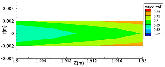
Figure 2.
Vapor void fraction cloud picture at the end of the pipe.
As shown in Figure 2, axially, the phase transition intensifies progressively, consistent with the Homogeneous Equilibrium Model (HEM) predictions. Radially, enhanced phase-change activity is observed near the pipe walls, showing clear wall-proximity dependence. The gas phase volume fraction of the pipeline centerline is smaller than the gas phase volume fraction of the pipe wall. This is because the pits, fine cracks, and cracks on the wall are most likely to become the vaporization core, making it easier to form bubbles.
3.3.2. Comparison of Critical Flow Rates
The mass flow rate in the pipeline is obtained by adjusting the outlet pressure without changing the inlet conditions. When the mass flow rate no longer changes with the outlet pressure, it is considered to reach the critical flow rate. Based on this approach, this article uses a one-dimensional homogeneous flow model for numerical solution and Fluent simulation to calculate the mass flow rate under different outlet pressures. The inlet pressure is 1 MPa, the inlet temperature is 213.61 K, and the diameter and length of the pipeline remain unchanged. The relationship between the pipeline mass flow rate and outlet pressure is shown in Figure 3, and the critical flow rate and critical pressure of the pipeline obtained by different methods are shown in Table 4.
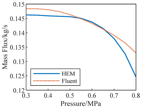
Figure 3.
Mass flow rate for different outlet pressures.
Table 4.
Mass flux under different outlet pressures.
Figure 3 and Table 4 show that the critical flow rates calculated by the two methods are relatively similar. In the process of solving a one-dimensional homogeneous flow model, given the mass flow rate, when a certain point is calculated, the equation system cannot be iteratively solved. At this point, given a sufficiently small pressure to reverse the length of the pipeline, the pipeline length is negative. According to the work of Kim [20], this point can be considered choked, and this point is the accumulation point. When the pressure of the injected storage tank is lower than the critical pressure, the flow rate in the pipeline no longer changes, and the outlet pressure no longer changes. At this time, the flow rate and pressure are the critical flow rate and critical pressure, respectively. Therefore, given a lower outlet pressure, the mass flow rate and critical pressure under given boundary conditions can be quickly obtained. As shown in Figure 3, when the pressure difference in the pipeline is small, the numerical calculation results of the one-dimensional homogeneous flow model are significantly different from those of Fluent, which may be related to the different values of relaxation factors under different outlet pressure conditions. The evaporation condensation model in Fluent uses the Lee model, but the Lee model overly relies on the selection of relaxation factors. In the absence of experimental data and previous examples for calculating liquid xenon two-phase flow, the selection of relaxation factors is highly unreliable, and the impact on the results is also uncertain.
4. Analysis and Discussion
By comparing the numerical calculation results of a one-dimensional homogeneous flow model with those of the Fluent simulation, it was verified that the calculation results are rational. Now, according to the one-dimensional homogeneous flow model, the influence of pipeline geometric parameters on the flash process is calculated and analyzed, and the dryness degree distribution of different working fluids along the pipeline is analyzed.
4.1. Influence of Pipeline Geometric Parameters on Flash Evaporation
Before designing the filling system, it is necessary to provide the geometric parameters of the pipeline, namely, the diameter and length of the pipeline. Therefore, it is necessary to study the effects of pipeline diameter and length on the flash evaporation process. When the geometric parameters of the pipeline change, the flow rate, the position of phase change points, and the distribution of dryness along the pipeline may change. According to Formulas (1) and (2), the diameter and length of the pipeline are the influencing factors of the flow rate and pressure drop in the single-phase flow section, while the length of the single-phase flow section is closely related to the position of the initial phase transition point. According to Formula (10), the specific enthalpy of the liquid and the latent heat of vaporization are the main factors affecting the dryness.
4.1.1. Impact of Pipeline Diameter on Flash Evaporation
As shown in Figure 4, the flow in the pipeline distinctly separates into two segments: a single-phase flow section and a two-phase flow section. The larger the pipeline diameter is, the smaller the pressure drop in the single-phase flow section, and the later the position of the phase transition point appears. According to Formula (1), increasing the diameter of the pipeline reduces the pressure drop in the single-phase flow section. Although the diameter increases and the flow rate in the pipeline also increases, the change in pressure drop in the single-phase flow section caused by the increase in flow rate is not as significant as the change in pressure drop in the single-phase flow section caused by the increase in diameter. Moreover, due to the increase in pipeline diameter, the pressure at the outlet of the 8 mm diameter pipeline is not equal to the back pressure, indicating that the flow has been blocked. Regardless of how the environmental pressure is reduced, the flow rate cannot increase, and flow parameters such as the pressure distributed along the pipeline will not change. In the absence of choked flow, the change in pipeline diameter does not affect the outlet dryness. This is because the pressure at the outlet is the same, so the liquid specific enthalpy and vaporization latent heat corresponding to this pressure are the same. According to Formula (10), the outlet dryness is almost the same.
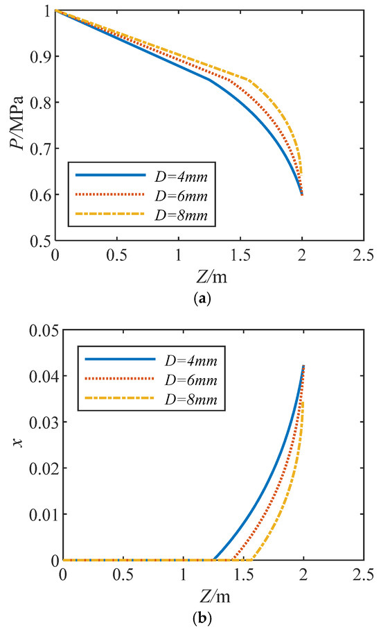
Figure 4.
Effect of diameter on the flow parameters. (a) Pressure distribution; (b) dryness distribution.
4.1.2. Impact of Pipeline Length on Flash Evaporation
The pressure and dryness degree distributions under different pipeline lengths are shown in Figure 5.
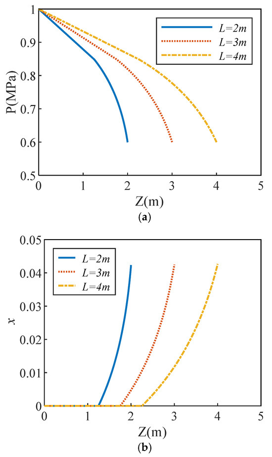
Figure 5.
Effect of length on the flow parameters. (a) Pressure distribution; (b) dryness distribution.
Figure 5b shows that the longer the pipeline is, the further the position of the phase change point is. This is because the mass flow rate corresponding to the long pipeline is lower, and the frictional pressure drop in the pipeline is smaller. Therefore, the length of the single-phase flow section is shorter, and the corresponding position of the initial phase change point appears farther. Since the pressure at the outlet has not changed, the specific enthalpy and latent heat of vaporization at the outlet are the same, and the dryness at the outlet has hardly changed. Therefore, the shorter the pipe length, the more intense the phase transition.
4.2. Comparison of Different Working Fluids
For two-phase flows with significant changes in physical parameters, low-temperature propellants and refrigerants have been extensively studied. Now, based on a one-dimensional homogeneous flow model, liquid xenon is compared with some refrigerants and low-temperature propellants to compare the flow parameter distributions of different working fluids under the same boundary conditions and analyze the similarities and differences among them. The pipeline has a length of 2 m, a diameter of 4 mm, and an absolute roughness of 0.002 mm. The inlet pressure of the different working fluids is 1 MPa, the inlet subcooling is 5 K, and the outlet pressure is 0.6 MPa. The inlet temperature conditions for different working fluids are shown in Table 5.
Table 5.
Conditions of inlet temperatures of different working media.
The physical parameters such as mass flow rate, density, and latent heat of vaporization of different working fluids in the pipeline are shown in Table 6.
Table 6.
Mass flux in the pipe of different working media.
The density and latent heat of vaporization refer to the liquid phase property parameters at the initial phase transition point, which are the ratios of the enthalpy change to the pressure difference from the initial point to the outlet. According to Formula (2), the higher the density is, the greater the mass flow rate in the pipeline.
Table 6 shows that in addition to refrigerants, other working fluids conform to this characteristic. As the density decreases, the mass flow rate in the pipeline decreases. The reason why the refrigerant R134a does not meet this characteristic is that the refrigerant has a high phase change mass transfer rate, and the average density inside the tube is lower than that of oxygen and nitrogen. According to Formula (10), a large enthalpy change and small latent heat of vaporization are beneficial for the phase transition. From the table, it can be seen that the refrigerant R134a is prone to phase transition, and xenon is also prone to phase transition. The distributions of the dryness and void fraction calculated for different working fluids along the pipeline are shown in Figure 6.
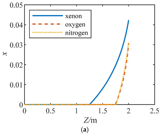
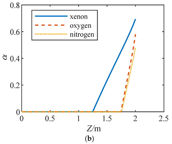
Figure 6.
Comparison of the gas rate along the pipe. (a) Dryness distribution; (b) void fraction distribution.
Figure 6 shows that the phase transition point of xenon occurs earlier than that of nitrogen and oxygen, and at the same location, the dryness and void fraction are greater. The dry degree distribution and void fraction distribution of nitrogen and oxygen are relatively close. This indicates that compared to low-temperature propellants such as liquid oxygen and liquid nitrogen, xenon has an earlier initial phase transition point and is more prone to flash evaporation. Moreover, the phase transition of xenon also becomes more intense.
The dryness and void fraction of different working fluids at the outlet were compared, and the dryness and void fraction of xenon at the outlet were considered unit 1. Table 7 lists R134a, the dryness and void fraction of liquid oxygen and liquid nitrogen at the outlet, and the ratio of dryness and void fraction of xenon at the outlet.
Table 7.
Specific values of the dryness and void fraction at the outlet of the pipe.
According to Table 7, at the outlet of the pipeline, the dryness of R134a is 2.34 times that of xenon, and the void fraction is 1.19 times that of xenon. The dryness of oxygen is 72% that of xenon, and the void fraction is 84% that of xenon; the dryness of nitrogen is 74% that of xenon, and the void fraction is 58% that of xenon. Compared to xenon, the refrigerant R134a is more prone to phase transition, while xenon is more prone to phase transition than are classic low-temperature propellants such as liquid nitrogen and liquid oxygen.
5. Conclusions
In the absence of experiments on xenon two-phase flow in pipelines caused by flash evaporation, this article adopts two methods for the numerical calculation of xenon two-phase flow in pipelines. The distributions of parameters such as pressure, dryness, and gas phase volume fraction along the pipeline were obtained. The main conclusions are as follows.
- (1)
- The similarities and differences between the one-dimensional homogeneous flow model and Fluent simulation methods are compared. The results calculated by the two methods are similar. It is also convenient to calculate the outlet pressure under critical flow and choked flow. Fluent can be used to calculate a two-dimensional distribution and display the entrance area, which can be used to obtain richer flow field information. The pipeline can be divided into single-phase and two-phase flow sections, where the two-phase flow section exhibits rapid pressure drop with a gas–liquid slip ratio of 1.
- (2)
- Increasing the diameter of the pipeline can extend the length of the single-phase flow section without changing the inlet pressure, inlet subcooling, or outlet pressure. Under the same conditions, increasing the length of the pipeline can extend the length of the single-phase flow section.
- (3)
- By using a one-dimensional homogeneous flow model, it is possible to compare the similarities and differences between liquid xenon and refrigerant, as well as between liquid xenon and low-temperature propellant flash evaporation. Refrigerant, liquid xenon, and low-temperature propellant are all working fluids that undergo significant changes in thermophysical parameters during flash evaporation, and their dryness and void fraction distributions in pipelines are similar. Compared to liquid oxygen and liquid nitrogen, liquid xenon is more prone to phase transition. Therefore, before refueling, it is necessary to precool the liquid xenon to increase its undercooling to suppress its phase transition and ensure the smooth progress of in-orbit refueling.
Author Contributions
Z.W. and C.J. wrote the main manuscript text. K.L. and Y.H. jointly supervised this work and modified the whole manuscript. G.L. and Y.C. prepared the figures and tables in this manuscript. All authors reviewed the manuscript. All authors have read and agreed to the published version of the manuscript.
Funding
This research is supported by the National Natural Science Foundation of China (Grant No. 52105290, 62373276 and 12172363).
Data Availability Statement
Data are contained within the article.
Conflicts of Interest
The authors declare no conflict of interest.
Nomenclature
| A | Cross-sectional area of the pipe (m2) |
| D | Diameter (m) |
| Friction coefficient | |
| G | Mass flow density (kg m−2 s−1) |
| h | Specific enthalpy (J kg−1) |
| L | Length of pipeline (m) |
| Mmass flow rate (kg s−1) | |
| Pressure (Pa) | |
| u | Velocity (m s−1) |
| x | Dryness |
| z | Pipe length (m) |
| Void fraction | |
| Density (kg m−3) | |
| Viscosity (Pa s−1) | |
| subscripts | |
| l | Liquid |
| g | Gas |
References
- Liao, Y.; Lucas, D. Computational modeling of flash boiling flows: A quality survey. Int. J. Heat Mass Transf. 2017, 111, 246–265. [Google Scholar] [CrossRef]
- Lin, S.; Kwok, C.C.K.; Li, R.Y.; Chen, Z.H.; Chen, Z.Y. Local frictional pressure drop during evaporation of R-12 through capillary tubes. Int. J. Multiph. Flow 1991, 17, 95–102. [Google Scholar] [CrossRef]
- Yin, P.; Yang, S.; Li, X.; Xu, M. Numerical simulation of in noise flow characteristics under flash boiling conditions. Int. J. Multiph. Flow 2020, 127, 103275. [Google Scholar] [CrossRef]
- Liang, S.M.; Wong, T.N. Numerical modeling of two phase reflective flow through adiabatic capillary tubes. Appl. Therm. Eng. 2001, 21, 1035–1048. [Google Scholar] [CrossRef]
- Seixlack, A.L.; Prata Á lvaro, T.; Melo, C. A two fluid model for reflective flow through adiabatic capillary tubes. J. Braz. Soc. Mech. Sci. Eng. 2013, 36, 1–12. [Google Scholar] [CrossRef]
- Zhu, J.; Elbel, S. CFD simulation of vortex flashing R134a flow expanded through convergint divergent noises. Int. J. Reflect. 2020, 112, 56–68. [Google Scholar] [CrossRef]
- Prajapati, Y.; Khan, M.K.; Pathak, M. Two phase VOF model for the reflective flow through adiabatic capillary tube. Ashrae Trans. 2014, 120, 60–67. [Google Scholar]
- Ingle, R.; Rao, V.S.; Mohan, L.S.; Dai, Y.; Inc, A.N.S.Y.S.; Chaudhry, G. Modeling of Flashing in Capillary Tubes using Homogeneous Equilibrium Approach. Procedia IUtam 2015, 15, 286–292. [Google Scholar] [CrossRef][Green Version]
- Luo, M.; Wang, T.; Zhang, Q.; Wang, N.; Chen, H.; Li, W. Investigation of Cryogenic Flashing Spreads. Astronaut. Syst. Eng. Technol. 2021, 5, 27–34+53. (In Chinese) [Google Scholar]
- Chauhan, V.; Saevarsdottir, G.; Tesfahunegn, Y.A.; Asbjornsson, E.; Gudjonsdottir, M. Computational study of two phase flashing flow in a calibrated geometric wellbore. Geophysics 2021, 97, 102239. [Google Scholar] [CrossRef]
- Li, Y.; Deng, J.; He, Y. Numerical study on non equilibrium condensation and flashing mechanisms in Rapid expansion process of transcritical CO2. CIESC J. 2022, 73, 2912–2923. (In Chinese) [Google Scholar] [CrossRef]
- Andreev, A.S.; Aksenchik, K.V. A Mathematical Model for the Operational Evaluation of the Dynamics of Heat and Mass Exchange in Flash Evaporators. Metallurgist 2024, 67, 1561–1569. [Google Scholar] [CrossRef]
- Gärtner, J.W.; Kronenburg, A. A novel ELSA model for flash evaporation. Int. J. Multiph. Flow 2024, 174, 104784. [Google Scholar] [CrossRef]
- Yang, Q.; Zhang, H.; Zhao, W.; Li, M.; Zhang, Z.; Li, X. Numerical simulation study on the spatiotemporal evolution characteristics of heat transfer in the static flash evaporation. Int. J. Therm. Sci. 2025, 210, 109675. [Google Scholar] [CrossRef]
- Darr, S.; Dong, J.; Glikin, N.; Hartwig, J.; Majumdar, A.; Leclair, A.; Chung, J. The effect of reduced gravity on cryogenic nitrogen boiling and pipe chilldown. NPJ Microgravity 2016, 2, 1–9. [Google Scholar] [CrossRef] [PubMed]
- Jiang, C. Thermomechanical Analysis of Xenon During On-orbit Refueling Process. Master’s Thesis, National University of Defense Technology, Changsha, China, 2019. (In Chinese). [Google Scholar]
- Lv, J.; Wu, Y.; Li, Z.; Song, Q.; Yang, R. Gas-Liquid Two-Phase Flow and Boiling Heat Transfer; Science Press: Beijing, China, 2017. (In Chinese) [Google Scholar]
- Ma, Y.; Li, Y.; Zhu, K.; Wang, Y.; Wang, L.; Tan, H. Investigation on no event filling process of liquid hydrogen tank under microgravity condition. Int. J. Hydrogen Energy 2017, 42, 8264–8277. [Google Scholar] [CrossRef]
- Lee, H.; Kharangate, C.; Mascarenhas, N.; Park, I.; Mudawar, I. Experimental and computational investigation of vertical downflow condensation. Int. J. Heat Mass Transf. 2015, 85, 865–879. [Google Scholar] [CrossRef]
- Kim, R. Computer aided design of a capillary tube for the expansion valve of the reflection machine. ASHRAE Trans. 1987, 93, 1362–1369. [Google Scholar]
Disclaimer/Publisher’s Note: The statements, opinions and data contained in all publications are solely those of the individual author(s) and contributor(s) and not of MDPI and/or the editor(s). MDPI and/or the editor(s) disclaim responsibility for any injury to people or property resulting from any ideas, methods, instructions or products referred to in the content. |
© 2025 by the authors. Licensee MDPI, Basel, Switzerland. This article is an open access article distributed under the terms and conditions of the Creative Commons Attribution (CC BY) license (https://creativecommons.org/licenses/by/4.0/).