Multi-Objective Optimization of Rocket-Type Pulse Detonation Engine Nozzles

Abstract

This numerical study addressed the multi-objective optimization of a rocket-type Pulse Detonation Engine nozzle. The Pulse Detonation Engine consisted of a constant length, constant diameter cylindrical section plus a nozzle that could be either convergent, divergent, or convergent–divergent. The space of five design variables contained: equivalence ratio of the H2-Air mixture, convergent contraction ratio, divergent expansion ratio, dimensionless nozzle length, and convergent to divergent length ratio. The unsteady Euler-type numerical solver was quasi-one-dimensional with variable cross-sectional area. Chemistry was simulated by means of a one-step global reaction. The solver was used to generate three coarse five-dimensional data tensors that contained: specific impulse based on fuel, total impulse, and nozzle surface area, for each configuration. The tensors were decomposed using the High Order singular Value Decomposition technique. The eigenvectors of the decompositions were used to generate continuous descriptions of the data tensors. A genetic algorithm plus a Gradient Method optimization algorithm acted on the densified data tensors. Five different objective functions were considered that involved specific impulse based on fuel, total impulse, and nozzle surface area either separately or in doublets/triplets. The results obtained were discussed, both qualitatively and quantitatively, in terms of the different objective functions. Design guidelines were provided that could be of interest in the growing area of Pulse Detonation Engine engineering applications.

1. Introduction

Pulse Detonation Engines (PDEs) are a promising propulsion plant option for some aerospace applications. The reasons might be twofold: (a) the concept has relatively low engineering complexity and (b) its thermodynamics cycle approaches the high-efficiency constant-volume heat addition limit. Significant developments have been reported during the past few years that involve flight testing, i.e., Buyakofu et al. [1] and Buyakofu et al. [2], and experimental testing, i.e., Bogoi et al. [3], and Oh et al. [4], among others. In this context, where practical applications are being addressed, engineering questions arise that focus on the improvement in PDE performance. Among many others, the most straightforward way of improving this performance could, possibly, be the implementation of an optimized nozzle. Another question that needs to be considered for flying platforms is to correlate the actual weight of the engine to its propulsive performance parameters.

A seminal experimental study in the field of nozzle optimization for PDE was the one published by Allgood et al. [5]. In this work, the authors studied different convergent (Con) and divergent (Di) bell-shaped nozzle geometries and provided guidelines regarding engine performance as a function of fill fraction and area ratio. The length (L) of their PDE was 1.88 m. Two diameters (D) were considered: 0.025 m and 0.051 m. Then, L/D = 1.4% to 2.8%. Nozzle length varied from 2% to 3% of the total length. The experiments of Yan et al. [6] addressed nine convergent–divergent (Con-Di) bell-shaped geometries with different contraction and expansion area ratios. The tube length and radius were 0.920 m and 0.030 m, respectively (L/D = 3.3%). Nozzle length varied between 65 mm and 107 mm. Within this space of design parameters, the authors identified the one that provided the maximum thrust augmentation (21%). Chen et al. [7] considered a 2.050 m long tube with a diameter equal to 0.136 m (L/D = 6.6%) equipped with Con, Di, and Con-Di nozzles. Their length varied between 188 mm and 210 mm. The experimental results showed that the performance of Con nozzles was worse than Di and Con-Di nozzles. Measured thrust augmentation ranged from 20% to 40%. Zhang et al. [8] considered 2 tubes and 21 nozzles with different shapes. The tube length varied between 0.660 m and 0.780 m. The diameter varied between 0.024 m and 0.030 m (L/D ~ 3.8%). The length of the convergent parts ranged from 0.010 m to 0.031 m. The length of the divergent parts was in the span from 0.024 m to 0.076 m. Their experimental tests showed that (a) most Con nozzles provided thrust augmentation when the fill fraction was larger than one, and (b) Di nozzles were better suited for fill fractions smaller than one. In one case, thrust augmentation was 25%. Ornano et al. [9] addressed the multi-fidelity geometry optimization (Con, Di, and Con-Di nozzles) of detonation combustors. Nozzle shapes were made up of five control points, Bezier curves. The parameter to be optimized was the nozzle exit force. The authors considered two types of optimization approaches. In the first case, they prescribed constant total pressure and temperature at the nozzle inlet section (i.e, no tube was considered), so the simulations had a steady character. In the second case, inlet profiles were time-dependent, so the simulations were unsteady. Two main conclusions were drawn from the study: (a) the optimum solution was the divergent nozzle, and (b) the inherent unsteadiness of PDT operation leads to optimum designs different from those obtained via the classical rocket engine approach. Zhang et al. [10] have explored the possibility of using fluidic solutions (Nitrogen injection) to adjust the effective area ratios. The authors reported thrust increments of the order of 100% in their experiments. A different type of nozzle configuration study has been reported recently by Kang et al. [11]. In this case, the objective was to study the acoustic characteristics of the PDE for different nozzle geometries.

The objective of the present study was to perform a systematic multi-design variables multi-objective nozzle optimization for a rocket-type PDE. Tube length and tube cross-sectional area were kept constant. A convergent–divergent nozzle was attached to its end. In all cases, the initial fresh mixture of reactants filled the tube only. The optimization involved five design variables: the equivalence ratio of the reactants, nozzle throat area, divergent exit area, length of the convergent section, and length of the divergent section. Optimum solutions were sought, accounting for different combinations of three global parameters of the PDE: total impulse, fuel-based specific impulse, and surface area of the nozzle (directly related to nozzle weight).

Previous studies performed by other authors (see previous paragraphs) have provided a large wealth of insight into the problem of nozzle optimization for PDE. These studies have tended to focus on single optimization objectives and considered a limited number of different design variables. Then, it is not easy to compare their conclusions. In this context, the novelty of the present study is to formulate and solve a problem that encompasses, albeit in an idealized way, different approaches proposed by previous authors, including, additionally, the issue of PDE weight. The goal is to address the problem of nozzle optimization in a multi-design parameter, multi-objective context that allows for the generalization of the results obtained within the frame of PDE design.

Regarding the organization of the manuscript, the sections are the following: Section 2: problem description, Section 3: flow simulation method, Section 4: optimization method, Section 5: results and discussion, and Section 6: conclusions.

2. Problem Description

A PDE was considered that consisted of a tube plus a convergent–divergent straight nozzle. The reactants were H2-Air. Initially, they filled the tube, not the nozzle. The tube length (L) was 1 m. The circular cross-section diameter (D) and area were 0.05 m and 0.002 m², respectively (D/L = 5%). These values were somewhat intermediate between the values used by Allgood et al. [5], Yan et al. [6], Chen et al. [7], Zhang et al. [8], and Ornano et al. [9], see

Table 1. Reactants, tube length (L), diameter (D), L/D ratio, and type of nozzle used in references [5,6,7,8,9] and in the present work. Con, Di, and Con-Di stand for convergent, divergent, and convergent–divergent, respectively.

Ref.	Reactants	L (m)	D (m)	D/L	Nozzle Type
Allgood et al. [5]	H2-Air	1.880	0.050	2.7%	Con, Di
Yan et al. [6]	Kerosene-O2	0.920	0.030	3.3%	Con-Di
Cheng et al. [7]	Gasoline-Air	2.050	0.068	3.3%	Con-Di, Con, Di
Zhang et al. [8]	Gasoline-Air	0.780	0.030	4.8%	Con-Di, Con, Di
Ornano et al. [9]	H2-Air	No tube			Con-Di, Con, Di
Present	H2-Air	1.000	0.050	5.0%	Con-Di, Con, Di

. The present study considered a single-cycle approach that was also the approach followed by Ornano et al. [9].

Five design variables were considered in the optimization. They, and their discretization in the space of variables, are defined in

Table 2. Definition and discretization of the design variables.

Design Variable	Definition	Discretization
Equivalence ratio	ϕ	0.8, 0.9, 1, 1.1, 1.2
Con-contraction ratio	λ1 = A7/A8	1, 1.8, 2.6, 3.4, 4.2, 5
Di-expansion ratio	λ2 = A9/A8	1, 2.4, 3.8, 5.2, 6.6, 8, 9.4, 10.8, 12.2, 13.6, 15
Nozzle length	λ3 = LN/L	0, 0.033, 0.066, 0.099, 0.132, 0.166, 0.2
Con-to-Di length ratio	λ4 = LCON/LDI	0, 0.2, 0.4, 0.6, 0.8, 1

.

Standard propulsion plant notation was used as follows: inlet, throat, and exit areas were denoted as A₇, A₈, and A₉, respectively. The total number of computed cases was 5 × 6 × 11 × 7 × 6 = 13,860. The data tensor generated in this way was coarse. Densification of the tensor suitable for optimization purposes was achieved via the surrogate modelling described in Section 4 (optimization method). A sketch of the PDE being considered is presented in Figure 1.

The optimization was carried out accounting for different combinations of the following objectives, as follows:

• Maximization of the specific impulse based on fuel: I_SPF (m/s);
• Maximization of the thrust time integral (total impulse): I_T (Ns);
• Minimization of the nozzle surface area: A_N (m²)

Five different optimization processes were considered. They are sketched in

Table 3. Definition of the five optimization cases. “X” denotes the objectives being addressed.

Optimization Case	ISPF	IT	AN
#1	X
#2		X
#3	X		X
#4		X	X
#5	X	X	X

where the “X” symbol signals the objectives addressed in each optimization. The rationale was to consider I_SPF and I_T separately, add A_N to each case, and, finally, consider the three objectives simultaneously.

3. Flow Simulation Method

The flow was described by a quasi-1D unsteady compressible reactive Euler equations, (Morris [12]).

$${\displaystyle \frac{\partial \mathit{W}}{\partial t}}+{\displaystyle \frac{1}{A}}{\displaystyle \frac{\partial \mathit{F}A}{\partial x}}=\mathit{Q}$$

(1)

$$\mathit{W}={\left[\rho ,\rho u,\rho E,\rho Y_k\right]}^T$$

(2)

where $\mathit{W}$ is the vector of conservative variables (density of the gas mixture, $\rho$, linear momentum, $\rho u$, total energy, $\rho E,$ and species densities, $\rho Y_k$) and $A$ stands for the $x$-dependent cross-sectional area of the tube and attached nozzle. Therefore, all conservative variables were the averaged values across the area $A\left(x\right)$. $Y_k$ stands for the mass fraction of each species $k$ in the mixture. For N species in the mixture,

$${\displaystyle \sum }_{k=1}^N{Y}_k=1,$$

(3)

$N-1$ mass fractions were solved. Thus, the number of equations to be considered was $N+3$. The specific total energy $E$ was defined as

$$E=h_s-{\displaystyle \frac{p}{\rho }}+{\displaystyle \frac{1}{2}}{u}^2$$

(4)

The sensible enthalpy $h_s$ functional dependence with temperature was

$$h_s={{\displaystyle \int }}_{T_0}^T{\displaystyle \sum }_{k=1}^N{c_p}_k^o{\displaystyle \frac{Y_k}{W_k}}dT$$

(5)

where $W_k$ is the molecular weight of species $k$. Molar constant pressure heat capacities ${c_p}_k^0$ were taken from Stull and Prophet [13] (JANAF polynomials).

$${c_p}_k^o=R_u{\displaystyle \sum }_{j=1}^5{a}_{j,k}{T}^{j-1}$$

(6)

Two sets of $a_{j,k}$ constant values for each species k were considered. The first set is valid in the temperature range from 200 K up to 1000 K and the second from 1000 K up to 5000 K. Relation between pressure and density in the mixture of $N$ ideal gases was modelled by the state equation as

$$p={\displaystyle \sum }_{k=1}^N{p}_k=T\rho R_u{\displaystyle \sum }_{k=1}^N{\displaystyle \frac{Y_k}{W_k}}$$

(7)

where $R_u$ is the universal gas constant. Flux vector $\mathit{F}$ and sources term $\mathit{Q}$ in Equation (1) were defined as

$$\mathit{F}={\left[\rho u,\rho u^2+p,\left(\rho E+p\right)u,\rho Y_{k}u\right]}^T$$

(8a)

$$\mathit{Q}={\left[0,{\displaystyle \frac{p}{A}}{\displaystyle \frac{dA}{dx}},{\dot{\omega }}_T,{\dot{\omega }}_k\right]}^T$$

(8b)

The source term of the energy equation was given by

$${\dot{\omega }}_T={\displaystyle \sum }_{k=1}^N{\dot{\omega }}_k\Delta {h_f}_k^o$$

(9)

where ${\dot{\omega }}_k$ and $\Delta {h_f}_k^o$ are the production/consumption rates of each specie and its formation enthalpy, respectively. The standard molar heat of formation for the species was obtained, also, from the JANAF polynomials, as follows:

$$\Delta {h_f}_k^o=R_u{a}_{6,k}$$

(10)

Combustion of $H_2$ in air was considered. A generic mechanism involving $N$ species could be described by $M$ elementary reactions of the following form:

$${\displaystyle \sum }_{k=1}^N{\nu }_{ki}^{\prime }\left[C_k\right]\rightleftarrows {\displaystyle \sum }_{k=1}^N{\nu }_{ki}^{\prime \prime }\left[C_k\right],fori=1,2,\dots ,M$$

(11)

where $\left[C_k\right]=\rho Y_k/W_k$ is the concentration of each species $k$. The arrows in Equation (11) represent, respectively, the forward $f$ and backward $b$ reactions, with $k_i^f$ and $k_i^b$ being the corresponding forward and backward rates constants. Then, each consumption/production rate of the specie $k$ related to reaction $i$ could be written as

$${\dot{\omega }}_{k,i}=\left({\nu }_{ki}^{\prime \prime }-{\nu }_{ki}^{\prime }\right)\left\{k_i^f{\displaystyle \prod }_{k=1}^N{\left[C_k\right]}^{{\nu }_{ki}^{\prime }}-k_i^b{\displaystyle \prod }_{k=1}^N{\left[C_k\right]}^{{\nu }_{ki}^{\prime \prime }}\right\}$$

(12)

Finally, the total consumption/production rate of the species $k$ in all involved reactions is written as

$${\dot{\omega }}_k=W_k{\displaystyle \sum }_{i=1}^M{\dot{\omega }}_{k,i}$$

(13)

In this work, a simplified chemical kinetic model with $N=$4 species ($N_2$, $O_2$, $H_2$, $H_{2}O$) described by the following one-step ($M=1$) irreversible global reaction was chosen, as follows:

$$2H_2+O_2+3.76N_2\to 2H_{2}O+3.76N_2$$

(14)

The irreversible Arrhenius reaction rate was

$$K_{glob}\left(T\right)=A{e}^{-{\displaystyle \frac{T_a}{T}}}$$

(15)

with pre-exponential factor and activation temperature equal to $A=1.4\times {10}^{13}{m}^3/kmols$ and $T_a=12995K,$ respectively, see McGough [14], Towery et al. [15], and Rai et al. [16].

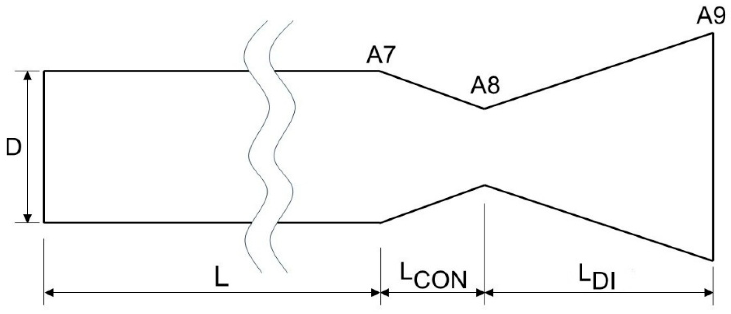
Regarding the geometry, Figure 2 shows a sketch of the cross-section distribution of $A\left(x\right)$. It could be observed that the domain had three sections: (1) tube ($L=1m$), (2) nozzle ($L_N={\lambda }_{3}L$), and (3) discharge region ($L_{DIS}=0.1m$, and $A_{10}/A_7=26,700$). The discharge region shape had a parabolic profile, ensuring a continuous derivative at the nozzle exit to prevent numerical instabilities.

The computational domain was initially at uniform pressure and temperature $p_0=101,325 \mathrm{Pa}$ and $T_0=300 \mathrm{K}$. The tube was initially filled with a fresh uniform mixture of $H_2$ and air ($O_2+3.76 N_2$) of equivalence ratio $\varphi$. The fresh mixture was assumed to initially be at rest. Detonations were numerically triggered by setting, i.e., initially, a small ignition region at $x=0$. Its length was equal to a single finite volume. The ignition pressure and temperature were $2\times {10}^{6 }\mathrm{Pa}$ and $3000\mathrm{K}$, respectively. The two assumptions of zero velocity for the initial fresh mixture and the setting of an initial small region to trigger ignition have been discussed previously by Sanchez de Leon et al. [17]. Initially, the nozzle and discharge section were filled with air. Zero velocity and zero gradient for the other variables were prescribed at the tube closed end,$x=0$. Ambient pressure, 1 bar, and zero gradients for velocity and temperature were prescribed at the discharge outlet section.

As for numerical implementation, the open-source framework OpenFOAM^® was used. This software uses Finite Volume Methods (FVMs) to solve the conservation equations of mass, linear momentum, energy, and mass species at every cell volume. The finite-volume density-based solver “rhoReactingCentralFoam” (a version of the standard OpenFOAM solver “rhoCentralFoam” that incorporates chemical reactions), developed to solve high-speed reactive flows, including detonations, McGough [14], was modified to implement the quasi-1D approach described in Equation (1).

Discretization of the convective terms was performed via a second order central-upwind scheme, Kurganov et al. [18]. Temporal discretization was carried out via an implicit Euler scheme. Equation (5) for temperature, which had an implicit character, was solved using a Newton–Raphson iterative approach. The stiff reaction terms were solved using a time-splitting method, which alternated between solving the homogeneous conservation laws without source terms (the fluid flow) and solving the conservation laws without convection (the chemistry). A fourth order Runge–Kutta scheme was selected as the time advancing algorithm for the chemistry model. An adaptative time step was set with a maximum Courant number of 0.1. The mesh size and the maximum Courant number were selected after a sensitivity analysis. The typical time step was $dt~2\times {10}^{-8}\mathrm{s}$. This time step was adjusted to ensure that the maximum Courant number did not exceed 0.1. Simulations were run up to the time when the static pressure at the tube closed end $x=0$ reached the initial pressure $p_0$. This condition defined the end time, $t_{end}$, of the simulation. The computation of each simulation case required an average of 40 min on a single core of an AMD Ryzen^TM 9 9900X processor.

Thrust, $F_x\left(t\right)$, total impulse, I_T, and specific impulse based on fuel, I_SPF, were computed as follows:

$$F_x\left(t\right)={\dot{m}}_9\left(t\right)\ast u_9\left(t\right)+A_9\ast \left(p_9\left(t\right)-p_{atm}\right)$$

(16)

$$I_T={{\displaystyle \int }}_0^{t_{end}}{F}_x\left(t\right)dt$$

(17)

$$I_{SPF}={\displaystyle \frac{I_T}{M_{F}g}}$$

(18)

where $M_F$ is the initial mass of fuel inside the PDE and $g=9.81 \mathrm{m}/{\mathrm{s}}^2$.

Regarding validation, the results were compared first, see

Table 4. Deviations in the present model with the Chapman–Jouguet (CJ) point obtained from the NASA’s Chemical Equilibrium with Applications (CEA) program, Gordon and McBride [18].

	NASA	Present	Deviation
${\mathrm{P}}_{\mathrm{CJ}}\left(\mathrm{bar}\right)$	15.7	15.9	1.5%
${\mathrm{T}}_{\mathrm{CJ}}\left(\mathrm{K}\right)$	2942	3285	10%
Wave Speed (m/s)	1968	2025	2.7%

, with reference data at the Chapman–Jouguet (CJ) point obtained from NASA’s Chemical Equilibrium with Applications (CEA) program, Gordon and McBride [19], for a stoichiometric mixture. It could be observed that pressure and wave speed are predicted with discrepancies smaller than 3%. Temperature deviations are larger (10%). The reason could be that the present simplified model lacks intermediate reactions and heat-absorbing species. Then, energy release is overestimated.

Second, the I_SPF for different equivalence ratios was compared to the experimental results of Shauer et al. [20] and the numerical results of Sanchez de Leon et al. [17], see Figure 3.

Third, the case presented by Ornano et al. [9], computed via the Method of Characteristics, was simulated. The steady-state force predicted by the present model was 5865 N, while Ornano et al. [9] reported a value of 5960 N (2% deviation).

Fourth, the work of Owens and Hanson [21] was simulated. The authors considered the combustion of ethylene in oxygen with a stoichiometric ratio in a PDE with a divergent nozzle. For the present model, the following single irreversible reaction was $C_2{H}_4+3O_2\to 2C{O}_2+2H_{2}O$. The reaction constants, taken from Xu and Konnov [22], were as follows: $A=1.2\times {10}^{13}{\mathrm{m}}^3/\mathrm{kmol}\mathrm{s}$ and $T_a=16,800\mathrm{K}$, see Equation (15). The results are summarized in

Table 5. Comparison of the present results and those of Owens and Hanson [21].

Parameter	Present	Owens and Hanson [21]	Deviation
Maximum Nozzle Force (N)	2950	3000	2%
Wave Detonation Time (ms)	0.515	0.550	6%
Blowdown Time (ms)	1.85	1.80	3%

. They are maximum nozzle force, wave detonation time (time for the detonation wave to reach the nozzle), and blowdown time.

With regard to numerical sensitivity,

Table 6. Results of the sensitivity analysis. The reference cases are highlighted in bold.

$\Delta \mathit{x}$ (μm)	Cells (×103)	CMAX	${\mathit{I}}_{\mathit{T}}$ (Ns)	ε (%)	${\mathit{I}}_{\mathit{S}\mathit{P}\mathit{F}}$ (s)	ε (%)	Wave Speed (m/s)	ε (%)	${\mathit{t}}_{\mathit{e}\mathit{n}\mathit{d}}$ (ms)	ε (%)
1300	1	0.1	1.88	0.5	4031	0.8	2078	0.5	5.99	1.3
866	1.5	0.1	1.90	0.5	4077	0.1	2073	0.2	6.03	0.7
650	2	0.1	1.89	0	4058	0.1	2073	0.2	6.04	0.5
520	2.5	0.1	1.89	0	4069	0.1	2073	0.2	6.06	0.2
433	3	0.1	1.89	0	4066	0.1	2068	0	6.06	0.2
371	3.5	0.1	1.89	0	4069	0.1	2068	0	6.07	0
325	4	0.1	1.89	0	4065	<0.1	2068	0	6.07	0
260	5	0.1	1.89	-	4063	-	2068	-	6.07	-
433	3	0.5	1.88	0.5	4048	0.4	2101	1.6	5.02	17.2
433	3	0.1	1.89	0	4066	0.1	2068	0	6.06	0
433	3	0.05	1.89	0	4063	0	2068	0	6.06	0
433	3	0.01	1.89	-	4063	-	2068	-	6.06	-

presents the sensitivity of the results obtained to mesh size and maximum Courant number allowed in the simulation, C_MAX, for a representative case with $\varphi =1 , {\lambda }_1=1.8, {\lambda }_2=2.4, {\lambda }_3=0.2 , \mathrm{and}{\lambda }_4=1$ (see Table 2). Variables to be compared were I_T, I_SPF, wave speed, and t_end. $\Delta x$ varied between 260 μm and 1300 μm. The number of cells varied between 1000 and 5000. C_MAX varied between 0.01 and 0.5.

The case with $\Delta x$ = 260 μm, 5000 cells, and C_MAX = 0. One was taken as the reference case (highlighted in bold in the upper part of the table) for sensitivity on cell size (number of cells). It could be observed that all cases with $260 \mathrm{\mu }\mathrm{m}<\Delta x<520 \mathrm{\mu }\mathrm{m}$ ($2500<number ofcells<5000)$ had discrepancies (ε) equal or smaller than 0.2%. The case with $\Delta x$ = 433 μm, 3000 cells, and C_MAX = 0.01 was taken as the reference case (highlighted in bold in the lower part of the table) for sensitivity on C_MAX. The case with C_MAX = 0.05 yielded the same results as the reference case. The case with C_MAX = 0.1 presented discrepancies of 0.1%. The case with C_MAX = 0.5 had an unacceptable discrepancy in t_end. Then, it could be considered that the results were converged whenever C_MAX ≤ 0.1. Accordingly, the parameters that were selected for the computations that represent a compromise between accuracy and computational load were $\Delta x=433 \mathrm{\mu }\mathrm{m}$, number of cells = 3000, and C_MAX = 0.1.

4. Optimization Method

Selection of the optimization method was driven by two factors: (1) computation of each simulation case required an average of 40 min, and (2) the problem being addressed involved five design variables.

As will be shown below, each optimization case required 20,300 computations of the objective function (20,300 simulations of the PDE). Since five different optimizations were considered, a total of 101,500 different cases had to be computed. Using a Ryzen 9 9900X processor with 24 cores, this would require a computational load of 93 days that was unfeasible for the authors. Then, a different approach, based on data tensor decomposition, was implemented to reduce the computational load. It came down, finally, to 15 days, which is an acceptable figure. This type of optimization methodology has been used previously by the authors, see Sastre et al. [23] and Sanchez de Leon et al. [17]. Then, the optimization method was organized into four steps, as follows:

• Step (1) Generation of the coarse data tensors;
• Step (2) Generation of the surrogate (densified) models of the data tensors;
• Step (3) Definition of the objective function;
• Step (4) Optimization algorithm.

Step (1) Generation of the coarse data tensors

First, the 13,860 cases defined in Table 2 were computed. Output parameters I_SPF and I_T were stored in two 5D tensors. The process did not apply to A_N because the nozzle surface area could be computed at any time at a negligible computational cost. The axes of the tensors were the following five design variables: ϕ, λ₁, λ₂, λ₃, and λ₄. Both the design variables ($x_i)$ and the output parameters ($y_i)$ were rendered dimensionless and normalized so that the optimization algorithm was well conditioned, as follows:

$${\tilde{x}}_i={\displaystyle \frac{x_i-x_{i\_min}}{x_{i\_max}-x_{i\_min}}},i=1,\dots ,5$$

(19)

$${\tilde{y}}_i={\displaystyle \frac{y_i-y_{i\_mean}}{y_{i\_max}-y_{i\_min}}},i=1,2$$

(20)

where $x_{i\_min}$ and $x_{i\_max}$ were minimum and maximum values of design variable $x_i$, and $y_{i\_mean}$, $y_{i\_max}$, and $y_{i\_min}$ were the mean, maximum, and minimum value of output $y_i$, respectively. With this normalization, design variables varied between 0 and 1, and output parameters vaired between −0.5 and 0.5.

Step (2) Generation of the surrogate (densified) model of the data tensor.

The coarse data tensors were decomposed via High Order Singular Value Decomposition, Tucker [24] and Lathauwer et al. [25,26]. The decomposition has the form

$$A^{\left(k\right)}=S^{\left(k\right)}\times U^{\left(1\right)}\times U^{\left(2\right)}\times \dots \times U^{\left(5\right)}$$

(21)

where $A^{\left(k\right)}$, $S^{\left(k\right)}$, and $U^{\left(i\right)}$ are the original coarse tensor $k$, the core tensor, and the eigenmode matrices that correspond to the five design variables. Once decomposition (21) was completed, third order splines were fitted to the eigenmodes, effectively generating a continuous surrogate-densified version of the original coarse data tensor. The optimization algorithm acted upon this surrogate data tensor.

To test the accuracy of the approach, 1400 test cases were computed via the surrogate model, and the results were compared to those obtained via direct simulation. These 1400 test cases were generated at random inside the space of design variables and neither of them belonged to the set of 13,860 cases used to generate the coarse data tensors. The results obtained were as follows:

• I_SPF. Mean relative error: 0.4%. Maximum error: 2.7%;
• I_T. Mean relative error: 0.4%. Maximum error: 2.8%.

The distribution of errors is shown in Figure 4. It could be observed that 66% of cases had an error smaller than 0.5%, 95% of cases smaller than 1%, and 99% of cases smaller than 2%.

Step (3) Definition of the objective function

The objective function, $\Psi$, (formulated for minimization) contained the three following terms:

$$\Psi =w_1\left(1-{\displaystyle \frac{I_{SPF}}{I_{SPF\_MAX}}}\right)+w_2\left(1-{\displaystyle \frac{I_T}{I_{T\_MAX}}}\right)+w_3\left({\displaystyle \frac{A_N}{A_{N\_MAX}}}\right)$$

(22)

where $I_{SPF\_MAX}$ and $I_{T\_MAX}$ represent the maximum values of the specific impulse and total impulse in the surrogate tensors, and $A_{N\_MAX}$ is the surface area of the nozzle with a maximum surface area. $w_1$, $w_2$, and $w_3$ were the weight factors to adjust the type of optimization. The coding of cases presented in Table 3 and weight factors were related as follows:

• Case #1. $w_1=1,w_2=0,w_3=0$;
• Case #2: $w_1=0,w_2=1,w_3=0$;
• Case #3: $w_1=1/2,w_2=0,w_3=1/2$;
• Case #4: $w_1=0,w_2=1/2,w_3=1/2$;
• Case #5: $w_1=1/3,w_2=1/3,w_3=1/3.$

Step (4) Optimization algorithm

The optimization algorithm involved the sequential application of a Genetic Algorithm (GA) plus a Gradient Method (GM). The objective function for both methods was obtained from the surrogate data tensor. The GA function of Matlab was used for the first step. The number of individuals in the population and the number of generations were 1000 and 20, respectively. The second step consisted of applying the Gradient Method-based FMINCON of Matlab to the leading individual obtained from the GA step. A maximum of 300 computations of the objective function was allowed to the GM. Accordingly, the number of steps was of the order of 20 (computing the Jacobian matrix in a 5D space requires the simulation of 10 points for each step, and the Hessian matrix needs to be computed, additionally, at some steps). In all cases, convergence (defined as a threshold for variation in the objective function) was achieved before the 300 computations were completed.

5. Results and Discussion

As detailed in Section 4, the optimization process was performed via a combined Genetic Algorithm plus a Gradient Method acting on the surrogate space of design variables. Given the heuristic nature of the Genetic Algorithm, it is recommended to repeat the optimization process many times to ensure that the best individual in the space of design variables is recovered. Then, each of the optimization cases #1 to #5 was repeated 1000 times. This was possible because, as explained in Section 4, the computational load is small due to the use of a surrogate space of design variables. As a matter of illustration, a histogram of the 1000 computations of case #5 is presented in Figure 5. It could be observed that the objective function values of 0.484, 0.481, and 0.480 were obtained 882 times, 15 times, and 103 times, respectively. Accordingly, the value of 0.484 was taken as the optimum.

The results obtained for the five optimization cases #1 to #5 defined in Table 3 are presented in

Table 7. Optimized nozzles associated with cases #1 to #5. D₉ is the diameter of section A₉.

	Case #1	Case #2	Case #3	Case #4	Case #5
	Optimization Objectives
	ISPF	IT	ISPF, AN	IT, AN	ISPF, IT, AN
ϕ	0.8	1	0.8	1	0.8
ISPF (m/s)	5194	4732	4654	4225	5189
IT (Ns)	2.06	2.21	1.84	1.97	2.06
LCON (m)	-	-	-	-	-
LDI (m)	0.2	0.2	-	0.02	0.2
LN/L	20%	20%	-	2%	20%
D9 (m)	0.056	0.057	-	0.053	0.053
D9/D	1.12	1.14	-	1.06	1.06
A9/A8	1.25	1.31	-	1.13	1.13
AN (m2)	0.033	0.033	-	0.003	0.032
APDE (m2)	0.192	0.192	0.159	0.162	0.191

below.

Before addressing the discussion of these results, it is convenient to summarize the results obtained by the other researchers referred to in Table 1. This summary is presented in

Table 8. Summary of the main results obtained by Allgood et al. [5], Yan et al. [6], Cheng et al. [7], Zhang et al. [8], and Ornano et al. [9]. It is indicated, also, whether the results are experimental (Exp) or numerical (Num). α stands for the fill fraction.

Reference	Main Results
Allgood et al. [5] (Exp)	Multi-cycle, 30 Hz. Thrust-based optimization. α < 0.5, optimum solution no-nozzle. α > 1, optimum solution Con nozzle.
Yan et al. [6] (Exp)	Multi-cycle, 10 Hz to 40 Hz. Thrust-based optimization. α ~ 0.7, optimum solution Con-Di nozzle of specific geometry (only Con-Di nozzles were considered).
Cheng et al. [7] (Exp)	Multi-cycle, 8 Hz to 15 Hz. Thrust-based optimization. Con-Di nozzle, Di nozzle, and straight tube deliver better performance than Con nozzle.
Zhang et al. [8] (Exp)	Multi-cycle, up to 100 Hz. Thrust-based optimization. α < 1, optimum solution Di nozzle. α > 1, optimum solution Con nozzle.
Ornano et al. [9] (Num)	Single cycle. Steady and unsteady force-based optimization. Optimum solution: Di nozzle with maximum area ratio.

.

The spread of the experimental results shown in Table 8 is large. This is possibly caused by the variety of experimental conditions and specificities of the test benches. For example, Allgood et al. [5] and Zhang et al. [8] agreed that the optimum solution was the Con nozzle when α > 1. However, for α < 1, Allgood et al. [5] recommended the straight tube while Zhang et al. [8] recommended the Di nozzle. In parallel, Cheng et al. [7] found that the Con-Di nozzle, Di nozzle, and straight tube delivered better performance than the Con nozzle. These somewhat contradictory conclusions might seem confusing, but it is to be said that similar discrepancies when addressing PDE nozzle performance were already noted in the review article of Kailasanath [27] back in 2003 (see the chapter titled “Nozzles for Pulse Detonation Engines” on page 153). More recently, Ornano et al. [9] were very clear when stating that in both single-cycle steady and unsteady state operation, the optimum is the Di nozzle with the largest area ratio. One of the possible phenomenological reasons could be that references [5,6,7,8] were multi-cycle while reference [9] was single cycle. This is related to the issue of single-cycle performance (neither purging nor filling) versus multi-cycle performance (sequential cycles that involve purging and filling). This problem was considered in detail by Ma et al. [28]. The authors modelled performance losses at high operation frequencies and concluded that above some frequency threshold, differences between single-cycle and multi-cycle analysis might have to be considered.

Another reason for the discrepancies could be that references [5,6,7,8] are experimental, while reference [9] is numerical. Obviously, from the methodological viewpoint, the numerical approach is cleaner in the sense that different physical effects could be isolated. However, in an actual test bench, real effects interact with each other, and the practical outcome is affected by these complex interactions. For example, two reasons of Allgood et al. [5] to propose the Con nozzle were back-pressurization and control the frequency of the engine. Also, Allgood et al. [5] suggested that purging and filling may not have a negligible effect on thrust performance. All this suggests that PDE performance is very sensitive to practical operating conditions.

Now, coming back to the present results shown in Table 7, the following aspects could be observed:

• In all cases, the optimum nozzle was divergent except in one case where the optimum solution was the straight tube;
• Optimizing in view of I_SPF and I_T separately with no regard for nozzle area (cases #1 and #2) led, basically, to the same nozzle geometry: largest allowable length and nearly the same diverging ratio D₉/D (less than 2% discrepancy). The difference was on the equivalence ratio: 0.8 for I_SPF optimization and 1 for I_T optimization, respectively. I_SPF in case #1 was 10% larger than in case #2. I_T in case #2 was 10% larger than in case #1;
• In all cases with the divergent nozzle, the diverging ratio was small: D₉/D < 1.12;
• Introduction of nozzle surface area (related to total PDE weight) in the optimization process substantially modified the optimum solution. In cases #3 and #4, the solution was the straight tube (the actual solution of case #4 was a very short divergent nozzle that yielded a PDE surface area that differed by a factor of 2% only from the straight tube);
• The comparison of cases #1 and #3 suggests that if the design team is willing to sacrifice 10% of I_SPF or 12% of I_T, the surface area of the PDE could be reduced by a factor of 17%. A similar conclusion could be drawn when comparing cases #2 and #4;
• Simultaneous optimization of I_SPF, I_T, and A_N (case #5) reverts to the solution of case #1 (optimization of I_SPF only). In cases #1 and #5, the relative importance of A_N in the optimization function is 0 and 33%, respectively, and this led to the same optimum nozzle. If the relative importance of A_N in the optimization function is increased to 50% (case #3), the optimum solution changes dramatically to the straight tube. This suggests that the topological space of optimum solutions depends sharply on the importance assigned to A_N in the optimization function;
• The results presented in Table 7 suggest that different options are possible depending on the terms present in the optimization function and on their relative importance. Also, although the divergent nozzle seems to be preferable in general terms, the simple solution of the straight tube has its own advantages and, accordingly, should not be discarded.

A way to visualize the behaviour of I_SPF and I_T as a function of the input parameters for the divergent nozzles, A_N, L_N, A₉/A₈, and ϕ, is presented in Figure 6 and Figure 7.

The following aspects could be observed in the figures:

• Larger equivalence ratios, ϕ~1, (blue dots) are preferable when optimizing I_T. Lean mixtures (ϕ~0.8) should be used when optimizing I_SPF;
• For any given L_N, both I_SPF and I_T have a maximum for some specific value of the parameter A₉/A_8. The tendency is similar for different values of ϕ. Unlike conventional rocket nozzles, where optimal performance is achieved when the exit pressure matches the ambient pressure, the present result shows that this principle does not necessarily apply to PDE. In particular, the presence of detonation waves creates a dynamic environment in which the classical nozzle optimization criterion is no longer valid. The difference arises from the fundamentally different nature of the flow in PDE, which is highly transient and nonlinear, unlike in steady or quasi-steady propulsion systems. The time-averaged outlet static pressure of all operation points plotted in Figure 6 and Figure 7 is presented in Figure 8, where the optima of the A₉/A₈ curves are highlighted with pink circles. It could be observed that all these optima are far above the dashed line that marks the ambient pressure of 1 bar. This indicates that the unsteady character of the rocket-type PDE disallows the use of conventional steady-state nozzle flow theory. This was already pointed out by Ornano et al. [9], although they reached the conclusion by other means;
• Increasing A₉/A₈ beyond this optimum has two negative effects: it increases the nozzle surface area, and it decreases both I_SPF and I_T;
• For very short nozzles, the curves A₉/A₈ are almost vertical, meaning that small variations in this parameter have a large negative impact on both I_SPF and I_T;
• If a least squares fitting is to be performed on the I_SPF-A_N and I_T-A_N data clouds of Figure 6 and Figure 7, it is easy to see that a dominant near-linear behavior could be observed. Also, it would be apparent that the slope would be small. For example, changing A_N from 0.02 m² to 0.04 m² (a 100% variation) would change I_SPF from, say, 4600 m/s to 5000 m/s (a 10% variation). That is, large variations in A_N entail smaller variations in I_SPF. This implies that the objective function is more sensitive to A_N than to I_SPF (or I_T), that is, precisely, what is observed in the results of Table 7.

6. Conclusions

When the objective function contained one performance parameter only (either specific impulse based on fuel or total impulse), the optimum solution was the divergent nozzle of the small area ratio (1.25 if the specific impulse based on fuel was considered, 1.31 if the total impulse was contemplated). In these cases, the nozzle length was the maximum allowed within the space of design variables (length equal to 20% of the tube length). If the nozzle surface area was added to the objective function (performance parameter and nozzle area having similar weights), the optimum solution switched to the straight tube. When the three criteria (specific impulse based on fuel, total impulse, and nozzle surface area) were put together in the objective function with similar weights, the optimum solution reverted to the divergent nozzle of the small area ratio (1.13). In this case, the two performance parameters had a combined weight of 2/3 in the objective function, while the weight of the nozzle surface area criterion was 1/3. These optimization results could be explained by the fact, observed in the densified data tensors, that large variations in A_N, of the order of 100%, entail smaller variations in I_SPF (or I_T), of the order of 10%, meaning that the objective function is more sensitive to A_N than to I_SPF (or I_T).

All this suggests that the nozzle design for rocket-type PDE is very sensitive to the criteria used for optimization. If propulsive performance is the single criterion, the divergent nozzle is the preferred solution. If, in addition, nozzle surface area (weight) is to be considered, the straight tube is the optimum solution. Broadly speaking, sacrificing 10% of the specific impulse based on fuel (or total impulse) allows for a total surface area reduction (tube plus nozzle) close to 20%. This suggests that, in a practical situation, the global architecture of a PDE might depend strongly on the type of mission. This is not surprising because it is a common feature of other propulsion plants.

Conventional steady-state nozzle flow theory should not be used for the design of Pulse Detonation Engines that present strongly unsteady behaviour. In fact, it was observed that actual performance maps present large differences, so Pulse Detonation Engine nozzles should be designed according to their unsteady character.

The practical operation of Pulse Detonation Engines depends critically on many design aspects of a very different nature. For instance, while this study and others support the convenience of the divergent nozzle, other studies propose the convergent nozzle based on control aspects of the multi-cycle operation of the engine. That is, engine optimization should be carried out, ideally accounting for both flow-related aspects and operational aspects. However, this may involve the difficult simultaneous presence of numerical and experimental approaches within the same optimization framework.