Genetic Algorithm for Optimal Control Design to Gust Response for Elastic Aircraft

Abstract

Developing control systems for high aspect ratio aircraft can be challenging due to the flexibility of the structure involved in the control loop design. A model-based approach can be straightforward to tune the control system parameters and, to this aim, a reliable aircraft flexible model is mandatory. This paper aims to present the approach pursued to design a control strategy considering the flexible aircraft simulator in the loop. Once the elastic model for the longitudinal dynamics has been set up, genetic algorithms are used to determine-together with a Linear Quadratic Regulator controller—a logic to improve the dynamic behaviour whilst encountering a gust. A relatively low order elastic model is developed for the dynamics in the longitudinal plane, including both rigid body and elastic degrees of freedom defined in a vehicle-fixed reference frame. The rigid body degrees of freedom and the associated states are the same as those of the rigid vehicle, whilst the additional states represent the elastic degrees of freedom. Modal characteristics are calculated from a finite element model of the aircraft using a commercial code, with the weight distribution added as lumped masses on grid points, while the aerodynamic rigid properties are described with a nonlinear database. Using the 2-D strip theory and neglecting the unsteady effects, the aeroelastic stability derivatives, i.e., elastic influence coefficients, are computed to superimpose the elastic effects on the rigid body degrees of freedom and vice versa. The flexible dynamics is compared to the rigid one in order to highlight the relevant changes in the aircraft modes. Following is herein proposed a control strategy combining genetic algorithms and Linear Quadratic Regulator controller to reduce the load factor, also considering the oscillation amplitude due to a deterministic gust encountered in a predefined flight condition.

1. Introduction

The main goal of the paper is to present the development of a controller for the response of a flexible aircraft to a gust. The first step is the modelling of the aircraft as a flexible body rather than a rigid one, in order to involve in the control loop design the elastic degrees of freedom (DoF), associated with the structural deformation. For instance, if the wing tip of an aircraft is equipped with sensors like strain-gauges or accelerometers, the output could be sent to a control logic to reduce the deformation of that part using moving control surfaces [1]. The latter reflects the basic working principle of Load Alleviation Logics (LALs), [2]. However, local loads can exceed the allowable loads of the structure and so the logic needs to be revised to comply with the constraints. Loads deriving from gusts are the ones closer to the corner points of the Allowable Loads Envelope (ALE) [3]) and the load factors deriving from gusts should be in the Allowable Flight Parameters Envelope within a certain tolerance. Moreover, the aircraft dynamic response to gust needs to be also evaluated against handling qualities [4,5], but it is out of the scope of the present paper.

With the aim to reduce the gust loads, the parameters to monitor are wing root bending and torque moments and the normal load factor ($n_z$) [6]. Generally speaking, load alleviation is performed through wing control surfaces, [7], to modify the lift distribution and thus reduce bending and torque moments. Moreover, the control surfaces on the aircraft tail need to be involved, to act on the rigid DoF and compensate the effect of the surface deflection on the aircraft motion [8]. Loads reduction allows to design lighter structures or to increase payload capability, as well as fuel storage, which in turn increases endurance. Moreover, the reduction of loads has a very large impact even on components’ life since, with smaller loads the residual fatigue life per number of cycles is increased [9]. Therefore, a suitable aircraft model is fundamental to design a control system for unconventional vehicle configuration, for instance a very high aspect ratio and slender structure, and to reduce the load factor due to gusts. Some issues can arise when the frequency separation between natural modes of the aircraft, dominated by the rigid-body DoF and those dominated by the elastic ones, is narrow [10,11]. In fact, when structural displacements occur at frequencies that are comparable to those of the rigid body modes, the coupling between the rigid body motion and the flexibility of the structure cannot be neglected and a proper model needs to be set up. The chosen methodology, depicted in Figure 1, is coherent with the traditional aeroelastic modelling approach with the equations derived in a vehicle-fixed body reference frame [12,13,14,15]. The present work deals with the design of a control strategy for a slender body aircraft, with aspect ratio close to 20, whilst it encounters a gust. The aspect ratio $AR$ is defined as:

$$AR={\displaystyle \frac{b^2}{S}}\simeq 20$$

(1)

where b is the wingspan and S the wing surface.

It is important to highlight that aircraft characteristics published herein are dimensionless because of company confidentiality. The structural displacements are considered small in order for the linear elastic theory to be applicable. The elastic modes are derived using a simplified finite element model and a commercial code, for the solution of the modal analysis.

The paper begins by introducing the notations and the reference frames used to derive the elastic contributions to the equations of motion. Here, Lagrange’s formulation is adopted to develop the governing equations of the elastic body using the generalised forces that are expressed as a function of the aerodynamic, propulsive and elastic coefficients through the principle of virtual work. The latter definition of the generalised forces introduces the coupling between the rigid-body and elastic DoF. This approach is used to derive a relative low order longitudinal elastic dynamic model of the aeroplane with the aim to evaluate a control strategy to be tuned on the flexible aircraft model for gust encountering. A Linear Quadratic Regulator (LQR) controller is adopted for the gust alleviation presented in this work. The genetic algorithms (GA) are used to optimise the controller parameters.

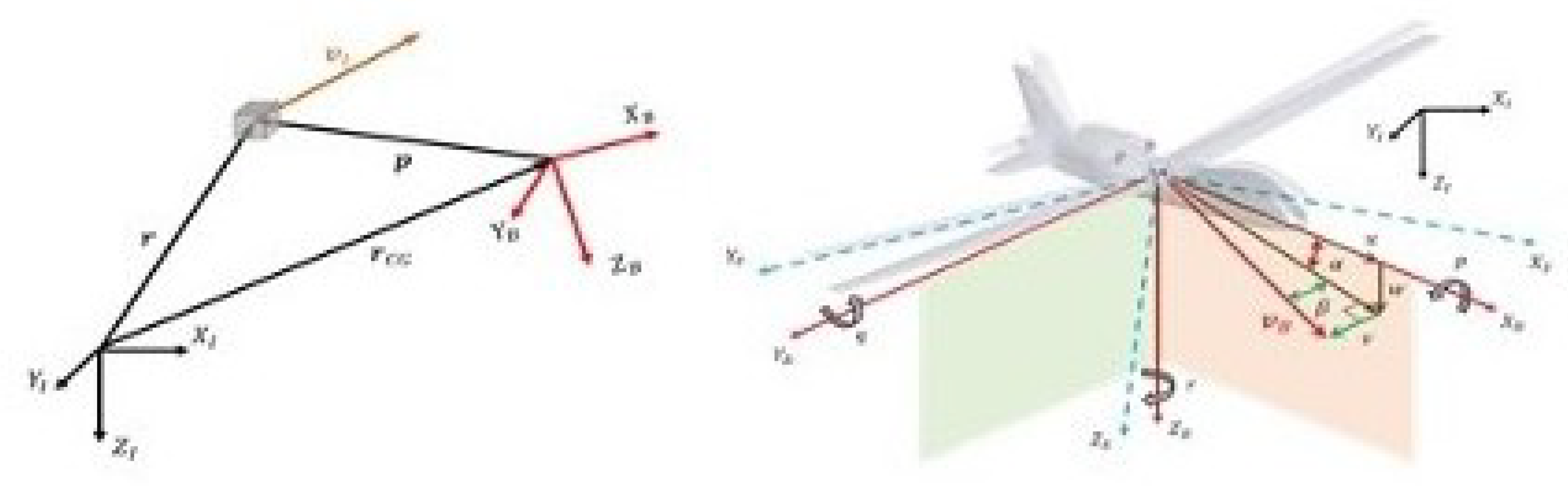
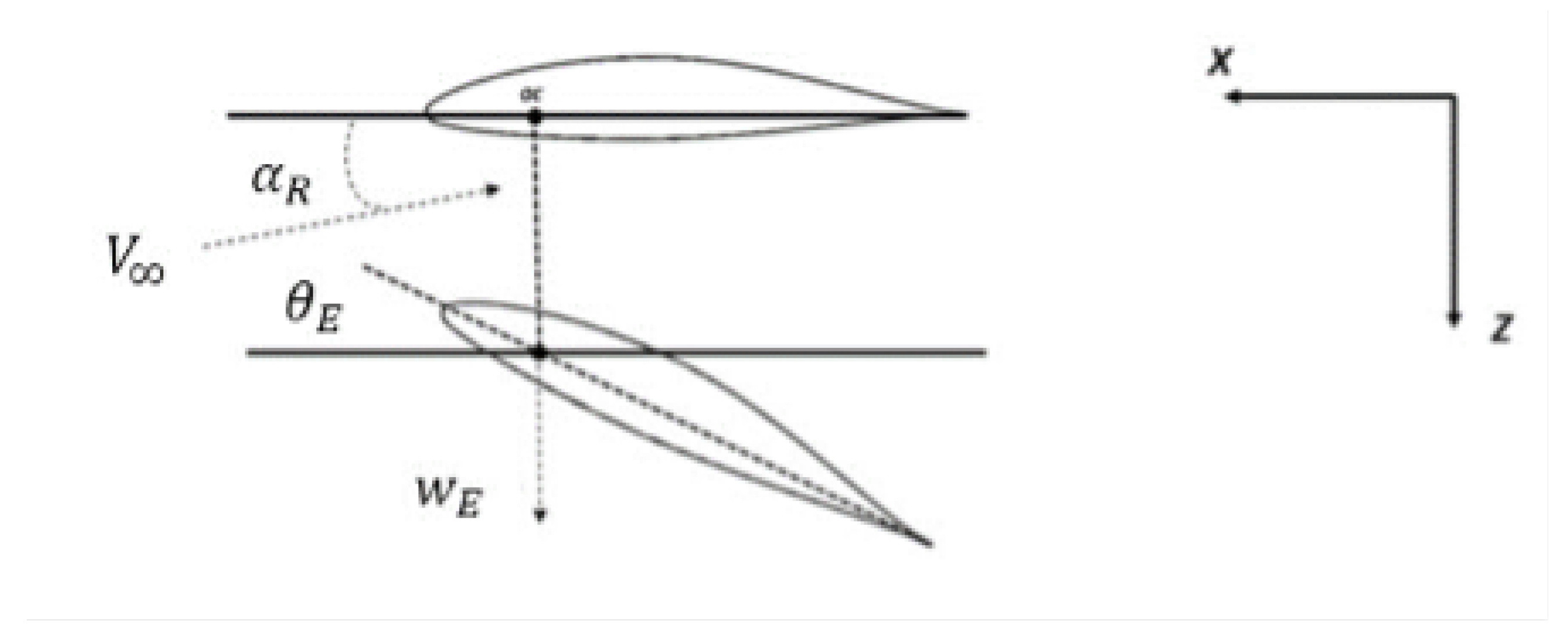
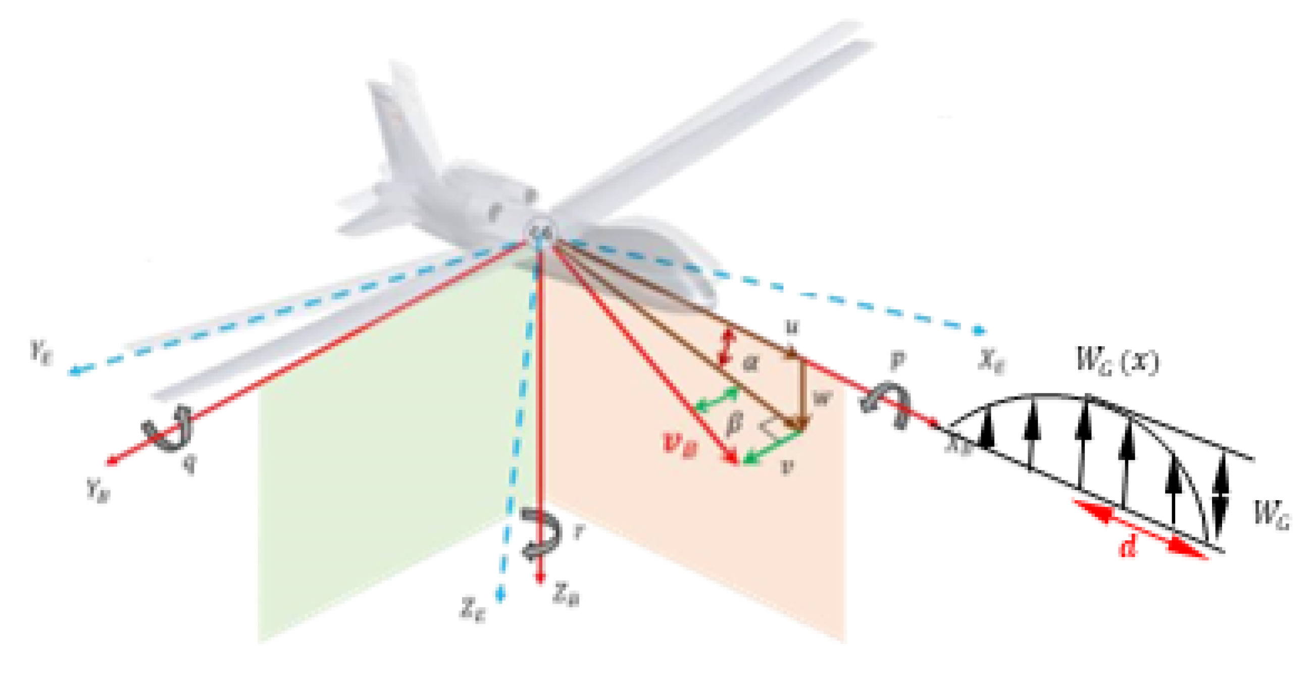
2. Notations and Reference Frames

In this work, vectors are indicated with bold lower case letters (e.g., $\mathit{v}$) and upper/lower case letters (e.g., V) are used for vector components, whereas the matrices are in bold capital letters (e.g., $\mathit{A}$).

An inertial reference frame ${\mathcal{F}}_I=\{X_I,Y_I,Z_I\}$ is considered. A vehicle-fixed and non-inertial reference frame ${\mathcal{F}}_B=\{X_B,Y_B,Z_B\}$, called body frame, is centred in the aircraft centre of gravity (CG) with axes oriented along fixed directions on board as described in Figure 2. The X-axis is contained in the symmetry plane and it is positive towards the aircraft nose; the Z-axis is contained in the symmetry plane and directed downward (i.e., from the upper to the lower wind surface); the Y-axis is defined to complete a left-handed coordinate system (i.e., towards the pilot’s right hand side) [16].

In ${\mathcal{F}}_I$, the position of a generic mass element, of density $\rho$ and volume $dV$, can be written as in (2) (see Figure 2).

$$\mathit{r}={\mathit{r}}_{CG}+\mathit{p}$$

(2)

If each point can be treated as a point-mass and assuming that ${\mathcal{F}}_B$ is rotating with angular speed $\mathit{\omega }=\{p,q,r\}$, in the inertial reference frame system ${\mathcal{F}}_I$, the velocity of the point can be determined as:

$${\displaystyle \frac{d\mathit{r}}{dt}}=\mathit{v}={\displaystyle \frac{d{\mathit{r}}_{CG}}{dt}}+{\displaystyle \frac{d\mathit{p}}{dt}}={\mathit{v}}_{CG}+\left({\displaystyle \frac{\partial \mathit{p}}{\partial t}}+\mathit{\omega }\times \mathit{p}\right)$$

(3)

where $\partial \left(·\right)/\partial t$ is the time derivative operator with respect to the vehicle-fixed reference frame, $d\left(·\right)/dt$ is the time derivative operator in the inertial reference frame and $v_{CG}$ is the velocity of the centre of gravity.

The aircraft attitude is expressed by the angle of attack (AoA, $\alpha$) and angle of sideslip (AoS, $\beta$) both defined as depicted in Figure 2.

Dealing with flexible aircraft, it is convenient to introduce a new reference frame which is non-inertial and time varying, ${\mathcal{F}}_E=\{X_E,Y_E,Z_E\}$, centred in the instantaneous aircraft CG, [10]; these are called mean axes. When considering the aircraft as rigid body, ${\mathcal{F}}_E\equiv {\mathcal{F}}_B$, whilst as the vehicle is regarded as deformable, the mean axes are anchored to the instantaneous centre of gravity. Thus this elastic frame follows the new aircraft configuration. Moreover, the mean axes frame is defined in order to have null linear and angular momenta due to elastic deformation at every instant. The latter definitions are based on the conditions of (4), defined as mean axes constraints.

$${\int }_{Vol}\left({\displaystyle \frac{d\mathit{p}}{dt}}\right)\rho dV={\int }_{Vol}\mathit{p}\times \left({\displaystyle \frac{\mathit{p}}{dt}}\right)\rho dV=0$$

(4)

Even though the exact constraints of (4) are not always easy to be applied, practical constraints can be derived [12].

The linear displacements are denoted using the notation $v_x$, $v_y$ or $v_z$, according to the axis along which the displacement occurs, whereas the rotational displacements are denoted using the variable $\theta$. For instance, the vertical displacements of the left wing are denoted as $v_{z_{wl}}$, the right wing rotation along the pitch axis is denoted as ${\theta }_{y_{wr}}$ whereas the only possible fuselage rotation around the roll axis is denoted as ${\theta }_f$. However, the only displacements taken into account are those of wing and tail.

Moreover, regarding the aircraft as flexible, the position of the generic point-mass $\mathit{p}$ in the vehicle fixed reference frame can be written as the sum of the position in the undeformed configuration, $\mathit{s}(x,y,z)$, and its instantaneous elastic displacement, ${\mathit{d}}_E(x,y,z,t)$, as reported in (5).

$$\mathit{p}=\mathit{s}+{\mathit{d}}_E$$

(5)

To conclude, as will be shown in later sections, ${\mathit{d}}_E(x,y,z,t)$ can be expressed with a modal expansion approach as a linear combination of the n free vibrational modal shapes of the structure, assuming n large enough [17].

3. Vehicle Description

The reference vehicle, depicted in Figure 3 as a stick model without engines, is a Leonardo Aircraft Division design study and it is characterised by an aspect ratio value close to 20. Due to the very slender and elongated wing structure, the flexibility of the aircraft is not negligible and so the elastic effects should be taken into account in the dynamic model.

Vehicle properties are reported in

Table 1. Normalised mass properties.

Property	Non-Dimensional Value
Mass	<10 tons
Roll moment of inertia	0.742
Pitch moment of inertia	0.245
Yaw moment of inertia	0.509

and

Table 2. Some wing nondimensional characteristics.

Property	Non-Dimensional Value
Wing span	18
Wing surface	26.67
$x_{CG}$ (distance from aircraft nose)	5.67

with normalised characteristics with respect to a reference value, because of company confidentiality.

The vehicle has a traditional control surface layout (i.e., slat, flap, aileron, elevator and rudder), however only the elevator deflection ${\delta }_E$ and the Power Lever Angle (PLA) commands have been taken into account in regards to the longitudinal dynamics. The same commands are used to trim the vehicle in the longitudinal plane.

Some rigid body trim conditions are depicted in Figure 4 as results of trimming the rigid aircraft model. The rigid aerodynamic database is non-linear and depends upon the angle of attack, the sideslip angle and the Mach number while the thrust is modelled as a function of Mach Number, altitude and PLA. Results, shown in Figure 4, refer to a condition of steady, straight and level flight for three different altitudes and in a certain velocity range using for trim only ${\delta }_E$ and PLA.

The rigid body trim characteristics show a behaviour similar to traditional aircraft parameters trends. The aerodynamic stability derivatives for the rigid model are computed from the aerodynamic database through linearisation around a trim condition. The trend of the natural frequencies $omeg{a}_n$ and the damping ratios $\zeta$ of the rigid body modes, as a function of airspeed, are depicted in Figure 5 for a fixed altitude.

In Figure 5, the natural frequencies for the two rigid body modes are normalised with respect to the maximum value, likewise for the damping ratio. For the short period mode, depicted with light blue circles, the natural frequency increases with airspeed, while the damping ratio decreases. However, this mode is a quite well damped e fast mode. On the other side, the phugoid mode, depicted with orange triangles, is unstable within a certain range of airspeed values and then remains slightly stable with a very low natural frequency.

The Argand diagram for the two rigid modes, depicted in Figure 6 for the same flight condition (altitude h of 1000 m and a speed V of 110 m/s) shows a behaviour similar to traditional aircraft rigid body modes.

4. Finite Element Model and Modal Solution

In order to evaluate the aeroelastic stability derivatives, i.e., the influence coefficients, a finite element model (FEM) has been set up to calculate modal characteristics, in particular the free-free elastic modes of the vehicle. The finite element model consists of grid points and lumped masses representing structural elements, fuel, engines and other systems. These grid points are connected through beam elements with properties indicated by the associated PBAR card of MSC NASTRAN and material properties indicated by the proper MAT card. Finally, connections between major components, i.e., wing with fuselage or empennage with fuselage, are realised using some rigid body element card implemented in Nastran. The finite element model, depicted in Figure 7, is used to calculate the modal properties of the aircraft through the SOL 103 of NASTRAN. The method chosen for eigenvalues extraction is the Lanczos method and modal shapes are normalised with respect to the maximum value of the eigenvalue component for each mode.

It is important to note that the structural reference frame, i.e., the frame used to build the FEM and shown in Figure 7, differs from the body fixed reference frame by a rotation of 180° around the y-axis.

The solutions of the modal analysis, i.e., natural frequencies and generalised masses and modal shapes, are reported in

Table 3. Normalised modal properties.

Elastic Modes Number	Normalised Natural Frequency ${\mathit{\omega }}_{\mathit{n}}$	Normalised Generalised Mass M	Modal Damping $\mathit{\zeta }$
1	0.285	0.769	0.02
2	0.579	0.788	0.02
3	0.629	0.769	0.02
4	0.802	1.000	0.02
5	1	0.639	0.02

for the first five elastic modes extracted. As stated before, the modal characteristics are properly normalised; for instance, the natural frequencies are divided by the greatest one among the relevant modes. The first five elastic modes reported in Table 3 have a natural frequency lower than 10 $\mathrm{Hz}$, in particular the first wing bending out-of-plane is less than 3 $\mathrm{Hz}$ while the first in-plane is less than 5 $\mathrm{Hz}$. These frequencies are close enough to those of the rigid body modes, thus the importance to study the effect of flexibility on the dynamics.

However, since in the following section we are dealing with the longitudinal dynamics of the aircraft only the symmetric elastic modes are taken into account to compute the aeroelastic stability derivatives.

Moreover, due to the aircraft symmetry with respect to the $X_B{Z}_B$ plane, we can consider an elastic mode as symmetric if it is symmetric with respect to the vehicle plane of symmetry. Since the generalized mass of some modes is quite low, these modes can be addressed as local instead of global. For instance, the elastic mode numbered with 1 in Table 3, depicted in Figure 8, is the first free-free vibration mode of the entire model but due to its low generalised mass, it can be referred to as the first out-of-plane wing bending moment. The modal displacement of wing and horizontal tail are then used to calculate the aeroelastic stability derivatives.

As can be seen from Figure 8 and Figure 9, the vertical displacements for wing and horizontal tail have an opposite sign as for the torsional rotation. Thus, as the wing bends upward and twists with leading edge downward, the horizontal tail bends downward and twists with leading edge upward. Note that, in order to show this behaviour in Figure 9, the vertical displacement and the torsional rotation have been multiplied by a certain gain with respect to the amplitude of Figure 8.

The second elastic mode is the anti-symmetric out-of-plane wing bending and it has been neglected, while the third elastic mode is a symmetric mode and can be referred to as the first in-plane wing bending, depicted in Figure 10 and Figure 11. Even if the aeroelastic stability derivatives are largely influenced by vertical displacement and torsional rotation of the elastic mode, and for the third mode the relevant displacement is in the longitudinal direction, this mode has been taken into account for their calculation for its low natural frequency.

Looking at Figure 11 it can be seen that wing vertical displacement scale is one order of magnitude lower than that of Figure 8. As previously said, the first elastic mode is a wing out-of-plane bending, with maximum displacement in the vertical direction, whilst the third mode is the first fore and aft wing bending with maximum displacement in the longitudinal direction. Moreover, wing and horizontal tail bending and twisting have again an opposite sign as for elastic mode number one. To conclude, these two elastic modes have been integrated in the rigid dynamic model to obtain the reduced order linear flexible one.

5. Equations of the Flexible Aircraft

Rigid body equations of motion are usually derived using a Newtonian approach; however, for the development of the equations governing the flexible body dynamics, the Lagrangian one has been used. Through this method, it is possible to show how body flexibility affects energy terms and how to take advantage of expressing elastic displacements using modal expansion and eigenvectors properties. The Lagrange equation is reported in (6).

$${\displaystyle \frac{d}{dt}}\left({\displaystyle \frac{\partial T}{\partial \dot{\mathit{q}}}}\right)-{\displaystyle \frac{\partial T}{\partial \mathit{q}}}+{\displaystyle \frac{\partial U}{\partial \mathit{q}}}={\mathit{Q}}^T$$

(6)

where:

• T is the flexible system kinetic energy
• U is the system potential energy
• $\mathit{q}$ is the generalised coordinate vector
• ${\mathit{Q}}^T$ is the vector of generalised forces acting on the vehicle

The term ${\mathit{Q}}^T$ can be expressed through the virtual work formulation, as reported in (7).

$${\mathit{Q}}^T={\displaystyle \frac{\partial \left(\delta W\right)}{\partial \left(\delta \mathit{q}\right)}}$$

(7)

where:

• $\delta W$ is the virtual work given by the external force acting on the system times the virtual displacement of its application point
• $\delta \mathit{q}$ is the generalised coordinate virtual displacement vector

Before further proceeding to define energetic terms involved in the Lagrangian formulation, the elastic displacement of a point of the structure is expressed using modal expansion. The elastic deformation ${\mathit{d}}_E$ of the body at a defined point $(x,y,z)$ at time t can be evaluated as a linear combination of the mode shapes $\nu (x,y,z)$ times the generalised coordinates $\eta \left(t\right)$, as reported in (8).

$${\mathit{d}}_E(x,y,z,t)=\sum _{i=1}^{\infty }{\mathit{\nu }}_i(x,y,z){\eta }_i\left(t\right)$$

(8)

The mode shapes to be used herein are those obtained from Nastran SOL103 and reported in Section 4. It is important to highlight that ${\eta }_i\left(t\right)$ is a scalar quantity while ${\mathit{\nu }}_i(x,y,z)$ is the vector of the i-th modal displacement along the reference axis. It is important to recall that the free-free vibration modes, both rigid and elastic, are mutually orthogonal functions with respect to the mass distribution. Thus, the practical mean axis constraints can be redefined and several simplifications can be made while expressing energetic terms. Recalling (3)–(5), the practical mean axes constraints become:

$${\int }_{Vol}\left({\displaystyle \frac{d{\mathit{d}}_E}{dt}}\right)\rho dV=0$$

(9)

$${\int }_{Vol}\left[\mathit{s}\times \left({\displaystyle \frac{d{\mathit{d}}_E}{dt}}\right)+{\mathit{d}}_E\times \left({\displaystyle \frac{d{\mathit{d}}_E}{dt}}\right)\right]\rho dV=0$$

(10)

These constraints can be further simplified assuming that elastic displacements and its time derivatives are small or even parallel, as for classical aeronautical structures, thus leading to (11).

$${\int }_{Vol}\left[{\mathit{d}}_E\times \left({\displaystyle \frac{d{\mathit{d}}_E}{dt}}\right)\right]\rho dV=0$$

(11)

Substituting the elastic displacement with a modal expansion in (9) and (10), leads to a new formulation for the practical mean axes constraint:

$${\int }_{Vol}\left({\displaystyle \frac{d{\mathit{d}}_E}{dt}}\right)\rho dV={\int }_{Vol}\left({\displaystyle \frac{d}{dt}}\sum _{i=1}^{\infty }{\mathit{\nu }}_i(x,y,z){\eta }_i\left(t\right)\right)\rho dV=\sum _{i=1}^{\infty }{\dot{\eta }}_i\left(t\right){\int }_{Vol}{\mathit{\nu }}_i(x,y,z)\rho dV$$

(12)

$${\int }_{Vol}\mathit{s}\times \left({\displaystyle \frac{d{\mathit{d}}_E}{dt}}\right)\rho dV=\sum _{i=1}^{\infty }{\dot{\eta }}_i\left(t\right){\int }_{Vol}\mathit{s}\times {\mathit{\nu }}_i(x,y,z)\rho dV$$

(13)

Integrals in (12) and (13) are equal to zero since the modal shapes are orthogonal to rigid rotations and translations with respect to mass distribution. These results can be used through energy terms formulation in order to obtain a straightforward derivation.

5.1. Dynamics of the Unconstrained Flexible Body

Considering (2) and (3), the kinetic energy of the body can be written as reported in (14).

$$\begin{array}{c}T={\displaystyle \frac{1}{2}}{\int }_{Vol}{\displaystyle \frac{d\mathit{r}}{dt}}·{\displaystyle \frac{d\mathit{r}}{dt}}\rho dV={\displaystyle \frac{1}{2}}{\int }_{Vol}\left[{\displaystyle \frac{d{\mathit{r}}_{CG}}{dt}}·{\displaystyle \frac{d{\mathit{r}}_{CG}}{dt}}+2{\displaystyle \frac{d{\mathit{r}}_{CG}}{dt}}·{\displaystyle \frac{\delta \mathit{p}}{\delta t}}+{\displaystyle \frac{\delta \mathit{p}}{\delta t}}·{\displaystyle \frac{\delta \mathit{p}}{\delta t}}+\right.\hfill \\ \hfill \hspace{1em}\hspace{1em}\hspace{1em}\hspace{1em}\hspace{1em}\hspace{1em}\hspace{1em}\hspace{1em}\left.+2{\displaystyle \frac{\delta \mathit{p}}{\delta t}}·\left(\mathit{\omega }\times \mathit{p}\right)+\left(\mathit{\omega }\times \mathit{p}\right)·\left(\mathit{\omega }\times \mathit{p}\right)+2\left(\mathit{\omega }\times \mathit{p}\right)·{\displaystyle \frac{d{\mathit{r}}_{CG}}{dt}}\right]\rho dV\end{array}$$

(14)

The kinetic energy consists of several terms, two of which are the translational and the rotational contribution, formally the same as for rigid aircraft. It is important to highlight that, for an elastic aircraft, the inertial tensor $\mathit{I}$ is no longer constant but varies due to elastic displacement. However, the first and second order effects deriving from elastic deformation on the inertia tensor can be neglected and so the inertial properties can be assumed constant throughout the derivation. Using the mean axes reference frame formulation and the properties of the free-free vibration modes, it is possible to further simplify the expression of the kinetic energy as:

$$\begin{array}{c}T={\displaystyle \frac{1}{2}}m{\mathit{v}}_{CG}·{\mathit{v}}_{CG}+{\displaystyle \frac{1}{2}}{\mathit{\omega }}^T\mathit{I}\mathit{\omega }+{\displaystyle \frac{1}{2}}{\int }_{Vol}{\displaystyle \frac{\delta \mathit{p}}{\delta t}}·{\displaystyle \frac{\delta \mathit{p}}{\delta t}}\rho dV=\hspace{1em}\hspace{1em}\hspace{1em}\hspace{1em}\hspace{1em}\hspace{1em}\hspace{1em}\hspace{1em}\hspace{1em}\hspace{1em}\hfill \\ ={\displaystyle \frac{1}{2}}m{\mathit{v}}_{CG}·{\mathit{v}}_{CG}+{\displaystyle \frac{1}{2}}{\mathit{\omega }}^T\mathit{I}\mathit{\omega }+{\displaystyle \frac{1}{2}}{\int }_{Vol}{\displaystyle \frac{\delta {\mathit{d}}_E}{\delta t}}·{\displaystyle \frac{\delta {\mathit{d}}_E}{\delta t}}\rho dV=\\ \hfill ={\displaystyle \frac{1}{2}}m{\mathit{v}}_{CG}·{\mathit{v}}_{CG}+{\displaystyle \frac{1}{2}}{\mathit{\omega }}^T\mathit{I}\mathit{\omega }+{\displaystyle \frac{1}{2}}\sum _{i=1}^n{M}_i{\dot{\mathit{\eta }}}_i^2\end{array}$$

(15)

where:

• $M_i$ is the modal mass of the i-th vibrating mode
• m is the mass of the aircraft

The kinetic energy is given by the sum of three decoupled contributions:

• A rigid translational kinetic energy term ($1/2m{\mathit{v}}_{CG}·{\mathit{v}}_{CG}$)
• A rigid rotational kinetic energy term ($1/2{\mathit{\omega }}^T\mathit{I}\mathit{\omega }$)
• A flexible kinetic term ($1/2{\sum }_{i=1}^n{M}_i{\dot{\mathit{\eta }}}_i^2$)

The potential energy U is given by the sum of gravitational potential energy $U_g$ and elastic strain energy $U_e$. The gravitational potential energy can be written as reported in (16), where $\mathit{g}$ is the gravitational acceleration.

$$U_g=-{\int }_{Vol}\mathit{g}·\mathit{r}\rho dV=-m\mathit{g}·{\mathit{r}}_{CG}$$

(16)

The potential energy due to the elastic deformation is linked to the external force work done on the structure from the undeformed reference shape to the deformed one. Considering the D’Alembert principle, the potential strain energy can be written as:

$$U_e=-{\displaystyle \frac{1}{2}}{\int }_{Vol}{\displaystyle \frac{d^2\mathit{r}}{d{t}^2}}·{\mathit{d}}_E\rho dV=-{\displaystyle \frac{1}{2}}{\int }_{Vol}{\displaystyle \frac{d^2{\mathit{d}}_E}{d{t}^2}}·{\mathit{d}}_E\rho dV$$

(17)

Again, expressing the elastic displacement with the modal expansion, we obtain:

$$U_e={\displaystyle \frac{1}{2}}\sum _{i=1}^n{M}_i{\omega }_i^2{\eta }_i^2$$

(18)

Before proceeding with the application of the Lagrange equation, a proper set of generalised coordinates, i.e., the vector $\mathit{q}$, needs to be defined. The generalised set of coordinates chosen as:

$$\mathit{q}={\{{\mathit{r}}_{CG},\varphi ,\theta ,\psi ,{\eta }_{i=1,\dots ,n}\}}^T$$

(19)

where:

• $\varphi$, $\theta$ and $\varphi$ are the Euler angles
• ${\eta }_i$ is the generalised coordinate associated with the i-th elastic degree of freedom

Once $\mathit{q}$ has been defined and the dependencies upon the relevant generalized coordinates has been shown in the energy terms, the Lagrange equation can be applied and the derivation follows as in [10]. The equations of motion describing the rigid body translation and rotation are formally the same as for the rigid aircraft dynamics and are reported, in vectorial form, in (20) and (21).

$$m({\dot{\mathit{v}}}_{CG}+\tilde{\mathit{\omega }}{\mathit{v}}_{CG})=\mathit{F}$$

(20)

$$\mathit{I}\dot{\mathit{\omega }}+\tilde{\mathit{\omega }}\mathit{I}\mathit{\omega }=\mathit{M}$$

(21)

where:

• $\mathit{F}=\{F_x,F_y,F_z\}$ is the vector of external forces acting on the vehicle
• $\mathit{M}=\{L,M,N\}$ is the vector of external moments acting on the vehicle
• $\tilde{\mathit{\omega }}$ is the cross-product matrix associated with $\mathit{\omega }$
• ${\mathit{v}}_{CG}=\{U,V,W\}$
• $\mathit{\omega }=\{P,Q,R\}$
• $\mathit{I}=\left[\begin{array}{ccc}{I}_{xx}& I_{xy}& I_{xz}\\ I_{yx}& I_{yy}& I_{yz}\\ I_{zx}& I_{zy}& I_{zz}\end{array}\right]$

The difference, with respect to the equations describing the rigid body dynamics, lies in the vector of the external forces and moments which, within the flexible aircraft frame, take into account the contribution given by the flexibility. For instance, the external forces vector is made up by three terms: aerodynamic plus inertial, propulsive and elastic ones. With the aforementioned assumptions and using the mean axis formulation, these terms are independent from each other. However, the terms linked to structure flexibility introduce the elastic DoF into the equations describing the dynamics of rigid body motion, thus coupling the two dynamics.

The elastic contribution to the external forces or moments can be calculated using the two-dimensional strip theory, once the variation of incidence due to elastic deformation is defined.

Figure 12 shows the elastic motion of an airfoil, at spanwise location y, relative to its undeformed configuration. The elastic deformation includes only local plunge velocity $w_E\left(y\right)$ and chord twist ${\theta }_E\left(y\right)$ of the aerodynamic centre (ac). The aerodynamic incidence at location y can be written as a sum of two contributions a rigid (subscript R) and an elastic term (subscript E) as reported in (22).

$$\alpha \left(y\right)={\alpha }_R\left(y\right)+{\alpha }_E\left(y\right)={\alpha }_R\left(y\right)+\left[{\theta }_E\left(y\right)+{\displaystyle \frac{w_E\left(y\right)}{V_{\infty }}}\right]$$

(22)

with $V_{\infty }$ indicating the freestream velocity vector.

Using the two-dimensional aerodynamic properties of the airfoil, it is possible to evaluate the elastic contribution to the overall external forces and moments. For instance, the elastic contribution to the lift generated by the wing deformation can be expressed as in (23).

$$L_{E_W}={\int }_{-\frac{b}{2}}^{\frac{b}{2}}{C}_{l_{{\alpha }_W}}\left({\theta }_{E_W}\left(y\right)+{\displaystyle \frac{w_{E_W}\left(y\right)}{V_{\infty }}}\right)q_W\left(y\right)c_W\left(y\right)dy$$

(23)

with:

• b wingspan
• $C_{l_{{\alpha }_W}}$ slope of the $C_l-\alpha$ of the airfoil of the wing at station y
• $q_W\left(y\right)$ wing dynamic pressure at station y
• $c_W\left(y\right)$ wing chord at station y

Similarly, the elastic wing contribution to the pitching moment can be expressed as:

$$M_{E_W}={\int }_{-\frac{b}{2}}^{\frac{b}{2}}{C}_{l_{{\alpha }_W}}\left({\theta }_{E_W}\left(y\right)+{\displaystyle \frac{w_{E_W}\left(y\right)}{V_{\infty }}}\right)\left(x_{ac}\left(y\right)-x_{cg}\right)q_W\left(y\right)c_W\left(y\right)dy$$

(24)

where:

• $x_{ac}\left(y\right)$ aerodynamic centre coordinate of the airfoil at station y, along the longitudinal axis
• $x_{cg}$ vehicle centre of gravity coordinate along X-axis

Local plunge velocity and elastic twist can be expressed in terms of modal shapes as:

$$w_E(y,t)={\dot{z}}_{ac}(y,t)=\sum _{i=1}^n{v}_{z_i}(x_{ac},y_{ac},z_{ac}){\dot{\eta }}_i\left(t\right)=\sum _{i=1}^n{v}_{z_i}\left(y\right){\dot{\eta }}_i\left(t\right)$$

(25)

$${\theta }_E(y,t)=\sum _{i=1}^n{v}_{z_i}^{\prime }\left(y\right){\dot{\eta }}_i\left(t\right)$$

(26)

Substituting these expressions in (23) and (24), it is possible to expand the elastic contributions as a linear combination of terms depending upon the i-th generalised coordinate and its time derivatives:

$$L_{E_W}=\sum _{i=1}^n\left({\displaystyle \frac{\partial L}{\partial {\eta }_i}}+{\displaystyle \frac{\partial L}{\partial {\dot{\eta }}_i}}\right)$$

(27)

$$M_{E_W}=\sum _{i=1}^n\left({\displaystyle \frac{\partial M}{\partial {\eta }_i}}+{\displaystyle \frac{\partial M}{\partial {\dot{\eta }}_i}}\right)$$

(28)

Finally, the equations governing the dynamics of elastic DoF are reported as:

$${\ddot{\eta }}_i+{\omega }_i^2{\eta }_i={\displaystyle \frac{Q_i}{m_i}}i=1,\dots ,n$$

(29)

In (29), the damping is not taken into account. $Q_i$ is the i-th component of the generalized force vector and it depends not only upon the elastic DoF, but also on the rigid ones, as expressed in (30).

$$Q_i=\left({\displaystyle \frac{1}{2}}\rho V_{\infty }^{2}Sc\right)C_{Q_i}=\left({\displaystyle \frac{1}{2}}\rho V_{\infty }^{2}Sc\right)f(\alpha ,q,{\delta }_E,{\eta }_i,{\dot{\eta }}_i)i=1,\dots ,n$$

(30)

Thus, through this term, the coupling between these two sets of DoF is once again established. An expression of $C_{Q_i}$ as a function of rigid and elastic DoF can be derived following chapter 7 in [10].

5.2. Linearised Flexible Dynamic Model

Starting from the overall set of the equations of motion for the flexible aircraft, a reduced one can be derived considering the evolution of the dynamics only in the longitudinal plane. Due to this constraint, as mentioned before, only the symmetric modes of vibration and the associated elastic DoF are taken into account. The nonlinear equations of motion describing the longitudinal dynamics are reported in (31). Here, an equation describing the dynamics of $\dot{H}$, altitude rate of change, has been added in order to consider different trim conditions.

$$\left\{\begin{array}{c}m\dot{U}=-QW-gsin\theta +F_{A_{X_R}}+F_{A_{X_E}}+F_{A_{X_P}}\hfill \\ m\dot{W}=QU+gcos\theta +F_{A_{Z_R}}+F_{A_{Z_E}}+F_{A_{Z_P}}\hfill \\ I_{YY}\dot{Q}=M_{A_R}+M_E+M_P\hfill \\ \dot{\theta }=Q\hfill \\ \dot{H}=Usin\theta -Wcos\theta \hfill \\ {\ddot{\eta }}_i=-2{\zeta }_i{\dot{\eta }}_i-{\omega }_i^2{\eta }_i+{\displaystyle \frac{Q_i}{M_i}}i=1,\dots ,n\hfill \end{array}\right.$$

(31)

For the scope of this study, the flexible model is set up integrating in the rigid one only two elastic modes and the dimensions of the linear dynamic model are increased by two states for each vibration mode included. Using the small perturbation theory, it is possible to linearise the previous system of equations in the neighbourhood of a trim condition. In this way, it is possible to study the model dynamic behaviour and how it is affected by the two elastic modes. Starting from (31), a linearised system is derived:

$$\left\{\begin{array}{c}\dot{u}=-W_{0}q-gcos{\theta }_0\theta +\frac{f_{A_{X_R}}+f_{A_{X_E}}+f_{A_{X_P}}}{m}\hfill \\ \dot{\alpha }=q-\frac{gsin{\theta }_0\theta }{U_0}+\frac{f_{A_{X_R}}+f_{A_{Z_E}}+f_{A_{Z_P}}}{m{U}_0}\hfill \\ \dot{q}=\frac{m_{A_R}+m_E+m_P}{I_{YY}}\hfill \\ \dot{\theta }=q\hfill \\ {\ddot{\mathit{\eta }}}_i=-2{\zeta }_i{\dot{\mathit{\eta }}}_i-{\omega }_i^2{\mathit{\eta }}_i+\frac{Q_i}{M_i}i=1,\dots ,n\hfill \end{array}\right.$$

(32)

In (32), the perturbation variables are reported in lower case; an exception is the perturbation of the generalised coordinate associated with the elastic degree of freedom that is reported in bold font. Finally, the subscript 0 is used to indicate the value of the variable in the reference condition.

The equation describing the linearised dynamics of the elastic DoF is second-order; thus, to set up a state space model, it should be written as two first-order equations. Applying a coordinate transformation, (33), it is possible to write the flexible dynamics as in (34).

$$\left\{\begin{array}{c}{\chi }_i={\eta }_i\hfill \\ {\chi }_{i+1}={\dot{\eta }}_i\hfill \end{array}\right.$$

(33)

$$\left\{\begin{array}{c}{\dot{\chi }}_i={\chi }_{i+1}\hfill \\ {\dot{\chi }}_{i+1}=-2{\zeta }_i{\omega }_i{\chi }_{i+1}-{\omega }_i^2{\chi }_i+\frac{Q_i}{M_i}\hfill \end{array}\right.$$

(34)

The state space vector, $\mathit{x}$, can be seen as an expansion of the state vector usually used for the longitudinal dynamics of a rigid aircraft, ${\mathit{x}}_R^T$, including the elastic DoF ${\mathit{x}}_E^T$.

$$\mathit{x}=\left[{\mathit{x}}_R^T{\mathit{x}}_E^T\right]=\left[u\alpha q\theta {\chi }_1{\chi }_2{\chi }_3{\chi }_4\right]\to \left[u\alpha q\theta {\eta }_1{\dot{\eta }}_1{\eta }_2{\dot{\eta }}_2\right]$$

(35)

The linearised elastic dynamic model can be expressed as:

$$\dot{\mathit{x}}=\mathit{A}\mathit{x}+\mathit{B}\mathit{u}$$

(36)

where the matrix $\mathit{A}$ is the state elastic matrix, $\mathit{B}$ is the input matrix and $\mathit{u}$ is the input vector made up of the elevator deflection and PLA command. Both matrices include rigid and elastic contributions. The state matrix $\mathit{A}$ can be partitioned in four sub-matrices as in (37) while the input matrix can be partitioned in two sub-matrices as in (38).

$$\mathit{A}=\left[\begin{array}{ll}{\mathit{A}}_{RR}& {\mathit{A}}_{RE}\\ ine{\mathit{A}}_{ER}& {\mathit{A}}_{EE}\end{array}\right]$$

(37)

$$\mathit{B}=\left[\begin{array}{c}{\mathit{B}}_{RR}\\ ine{\mathit{B}}_{ER}\end{array}\right]$$

(38)

In the notation used to indicate the sub-matrices, for the state and for the input matrices, the two subscripts refer to the two different set of elastic DoF. For instance, the sub-matrix ${\mathit{A}}_{RR}$ expresses the effect of the rigid DoF on the same set whilst ${\mathit{A}}_{RE}$ describes the effect of the elastic DoF dynamics on the rigid one.

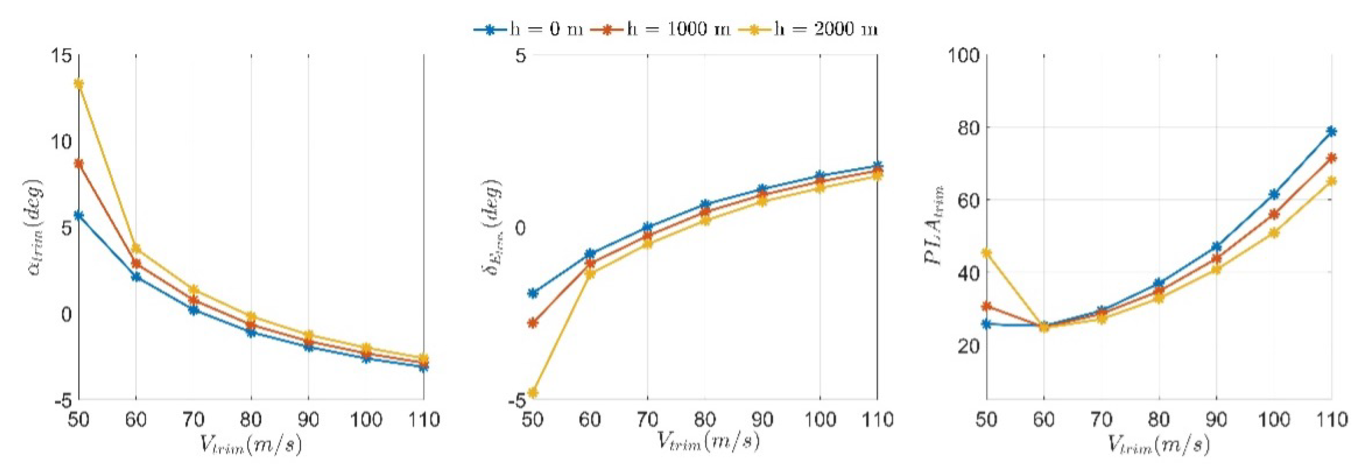
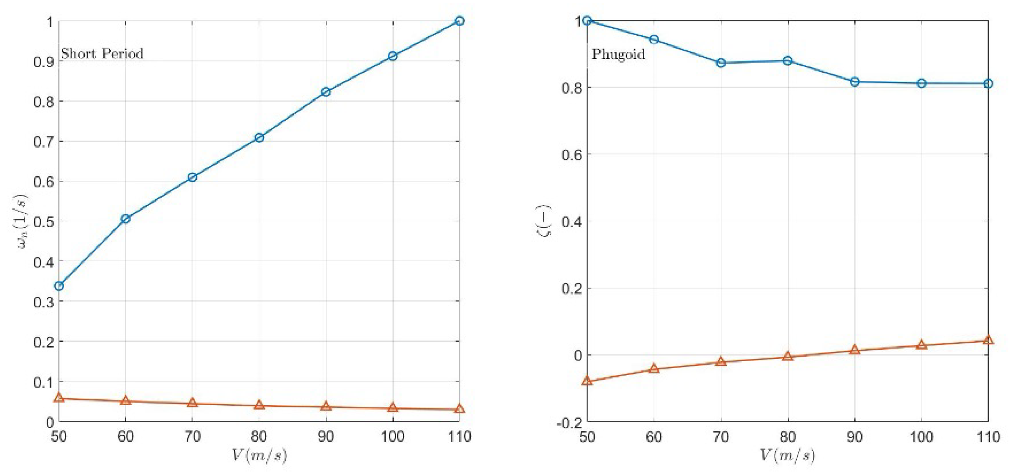
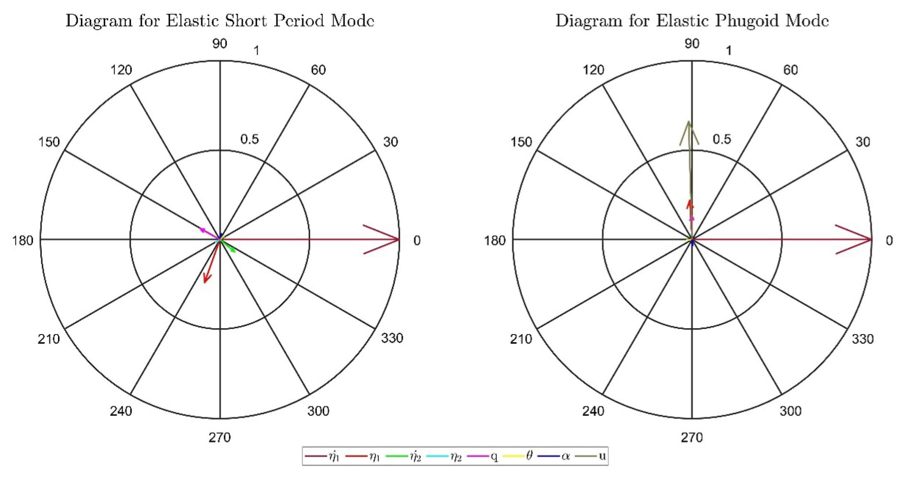
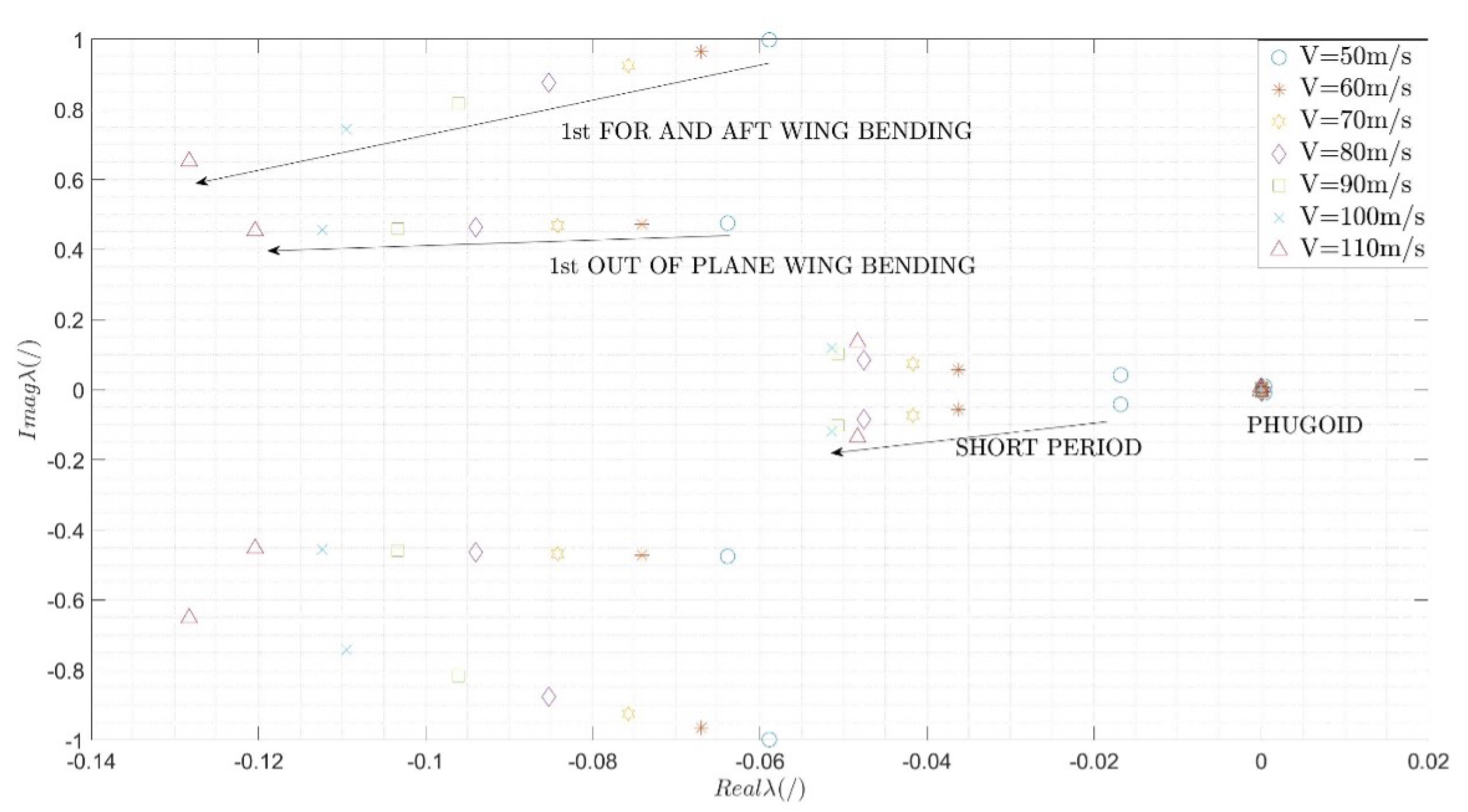
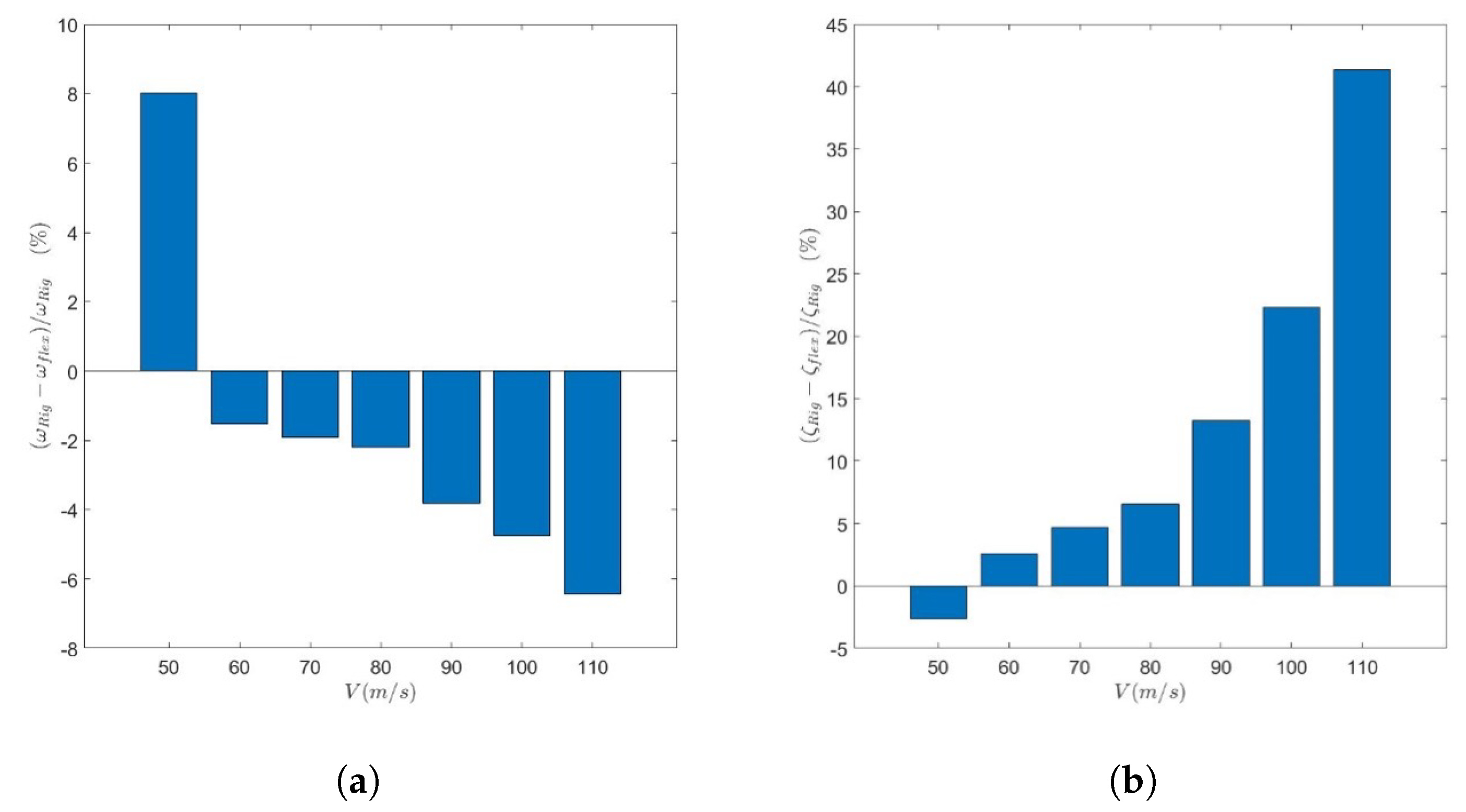
5.3. Numerical Results

The matrix $\mathit{A}$ is of order eight and, therefore, the dynamics are characterised by eight eigenvalues, representative of four modes. Two of them are the vibration modes integrated in the rigid model and the other two are those associated with the rigid body degree of freedom. However, the modes of the elastic aircraft related to rigid body DoF are not the same as for the rigid dynamic model due to the elastic states. For instance, in Figure 13 as for Figure 6, the Argand Diagram is shown for the eigenvectors associated with the rigid body modes.

The so-called Elastic Short Period Mode is strongly affected by the evolution of the four elastic states and the rigid body DoF are barely visible. Thus, a strong coupling exists between the two elastic modes and the fastest rigid mode associated to the rigid DoF. As a consequence, a classical short period mode is no longer recognisable. Figure 14 shows the root locus of the linear elastic system for a fixed altitude of 1000 $\mathrm{m}$. The eigenvalues in the root locus are normalized with respect to the eigenvalue with maximum modulus because of company IP protection. The poles associated with the short period mode are affected by the presence of the elastic poles rather than those of the phugoid mode. In fact, the two rigid body modes do not approach each other but the short period poles follow the poles of the elastic modes while they are moving in a more stable region.

The variation of the natural frequency and of the damping ratio, at a fixed altitude, of the short period mode between rigid and elastic model is reported in Figure 15. For the natural frequency with increasing velocity, the short period of the elastic model becomes faster. The increase in the natural frequency reaches around 10% at the maximum trim velocity analysed. Instead, for the damping ratio, an opposite trend can be seen, i.e., the short period for the elastic model becomes less damped at higher velocity (40% less at maximum trim velocity).

For the Elastic Phugoid Mode in Figure 13, a similar behaviour to the rigid one can be observed, as in Figure 6. In fact, from Figure 14 the phugoid still remains in a very small neighbourhood of its initial position. Since the phugoid dynamic characteristics are very close to zero, a diagram similar to Figure 15 is not reproduced.

To conclude, in order to see how elastic modes affect the design of a controller, only those closer to the rigid ones are taken into account, considering the development of a relatively low order model.

Figure 16 shows the trim condition, for the same parameters considered in Section 3, for both rigid and elastic aircraft. At a fixed altitude, it can be seen that the angle of attack needed to trim the aircraft in a steady state and straight level flight is slightly different for the two models and, in particular, the elastic aircraft seems to develop a greater lift and the elevator deflection varies as a consequence. The PLA command is slightly affected by the elastic effects since we have neglected any change in the aerodynamic drag.

6. Control Strategy for Gust Effect Reduction

In this section, a control strategy combining GA and LQR is proposed to reduce the effects of a vertical gust, i.e., reduction of the induced normal load factor. The type of gust considered is a deterministic one supposed to be encountered in straight and level flight.

The GA strategy [18] is used to drive the optimal selection of the weights of the LQR matrices in order to obtain the best gains. In setting up the GA algorithm, an objective function is defined together with some boundaries related to same properties of the weight matrices of the LQR.

In Section 6.3, the LQR controller is designed, [19], considering the state weight matrix as diagonal. Its coefficients are determined using a trial and error approach, showing good results. In Section 6.4, when the GA is coupled with LQR, the matrix Q is taken as full and its coefficients are evaluated through the GA optimisation. Moreover, in Section 6.4, in order to simulate the time delay in command actuation, a first order model is introduced.

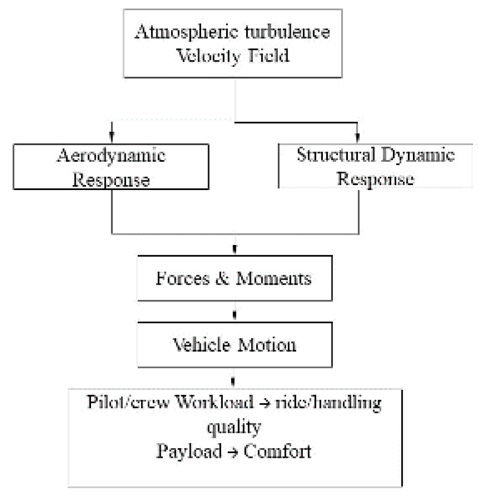
6.1. Gust Effects: Background

Aircraft dynamics are usually triggered in simulation not only with pilot commands but with inputs that are somehow representative of atmospheric gust/turbulence. This type of external influence is useful to determine whether the loads generated on aircraft components are within their allowable strength limits, so as to provide design/fatigue loads [20], or if the dynamic behaviour reaches an acceptable level of handling qualities [21].

Studies have shown that, in real scenarios, aircraft are unlikely to encounter a turbulence of constant intensity, [4]. The effects of gust/turbulence were estensively studied in the past using as guideline the MIL-A-8861B [22] considering as design load the combination of a steady level 1-g flight and the increment due to gust. Depending on aircraft category, certification specifications ([23,24]) are used to evaluate aircraft loads and handling qualities in order to assess its compliance for gust/turbulence. Recently, in the 7th ALEF (Aerodynamic Loads Estimation at extremes of the Flight envelope [25]) framework, new methodologies were developed to estimate gust effects in terms of loads and handling qualities. These methodologies involve the application of high fidelity CFD (Computational Fluid Dynamic)/RANS (Reynold Avarage Navier Stokes) approaches coupled with high order aero-elastic theory.

Usually, a rigid aircraft model is used to analyse an aircraft’s response to gust, while in this work a linear reduced flexible dynamic model is used. This can be seen as an approach to simulate the dynamic response of the aircraft structure to the velocity field encountered during gust. In fact, the structural response affects the aerodynamic forces and moments developed by the lifting surfaces and, as a consequence, the ride and handling qualities. In Figure 17, an outline of the gust dynamics is reported. For our analysis, a deterministic approach is used to evaluate the effects of the gust on aircraft dynamics. In particular, a discrete vertical gust of type ‘1-cos’ is used as an input to trigger the dynamics in the longitudinal plane. Moreover, gust effects are regarded to be the output of a variation in the angle of attack due to the combination of the aircraft velocity and gust velocity profile (see Figure 18). Other fundamental hypothesis on gust analysis can be further explored in [21] Section 9 and in [20].

In the following section, gust effects on aircraft dynamics are evaluated considering different approximations of the linear model, i.e., pure plunge/short period approximation/flexible dynamics. Considering the linear dynamic model of the vehicle in a state-space representation to evaluate the gust effects two control inputs are defined:

• ${\alpha }_G$: angle of attack due to a gust velocity profile
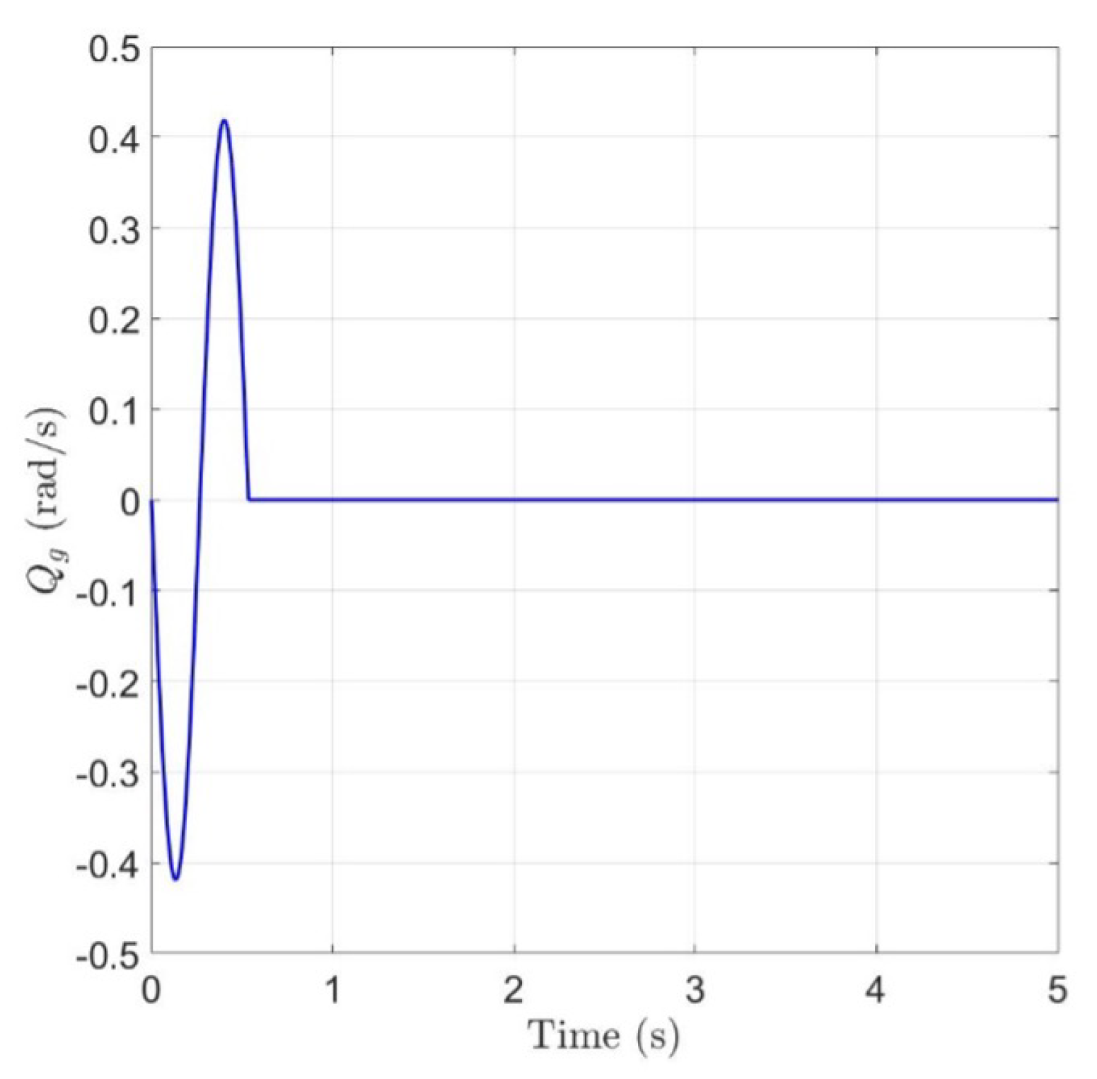
• $Q_G$: pitching angular velocity due to a gust profile

The vertical velocity profile of a discrete gust of one minus cosine type, reported in (39), will be supposed frozen in space while the aircraft goes through it.

$$w_G\left(x\right)=w_G\left(1-cos{\displaystyle \frac{\pi x}{d}}\right)$$

(39)

where

• $w_G$ is the magnitude of the vertical gust profile
• d is the gradient distance defined as a linear function of the wing chord

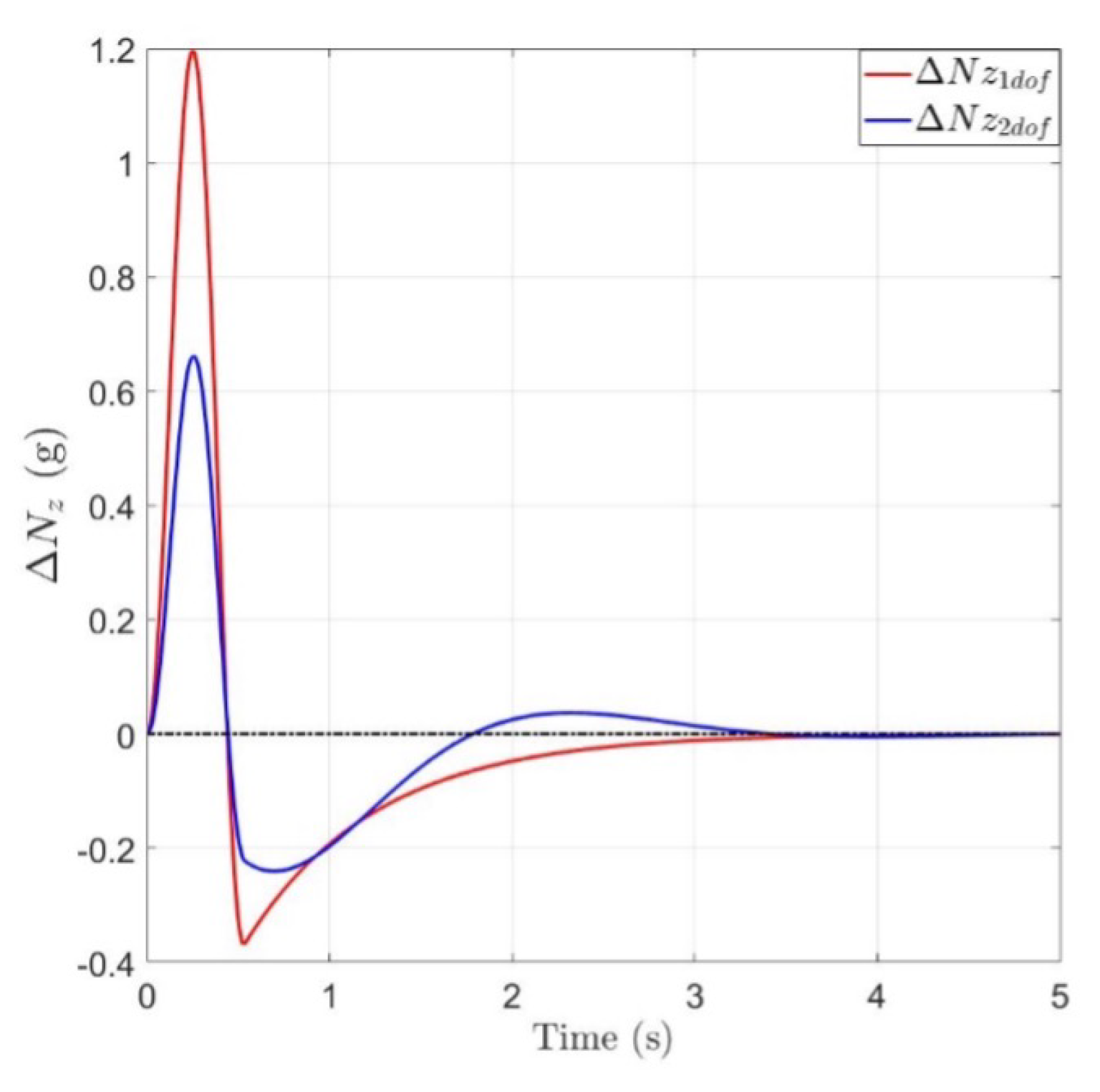
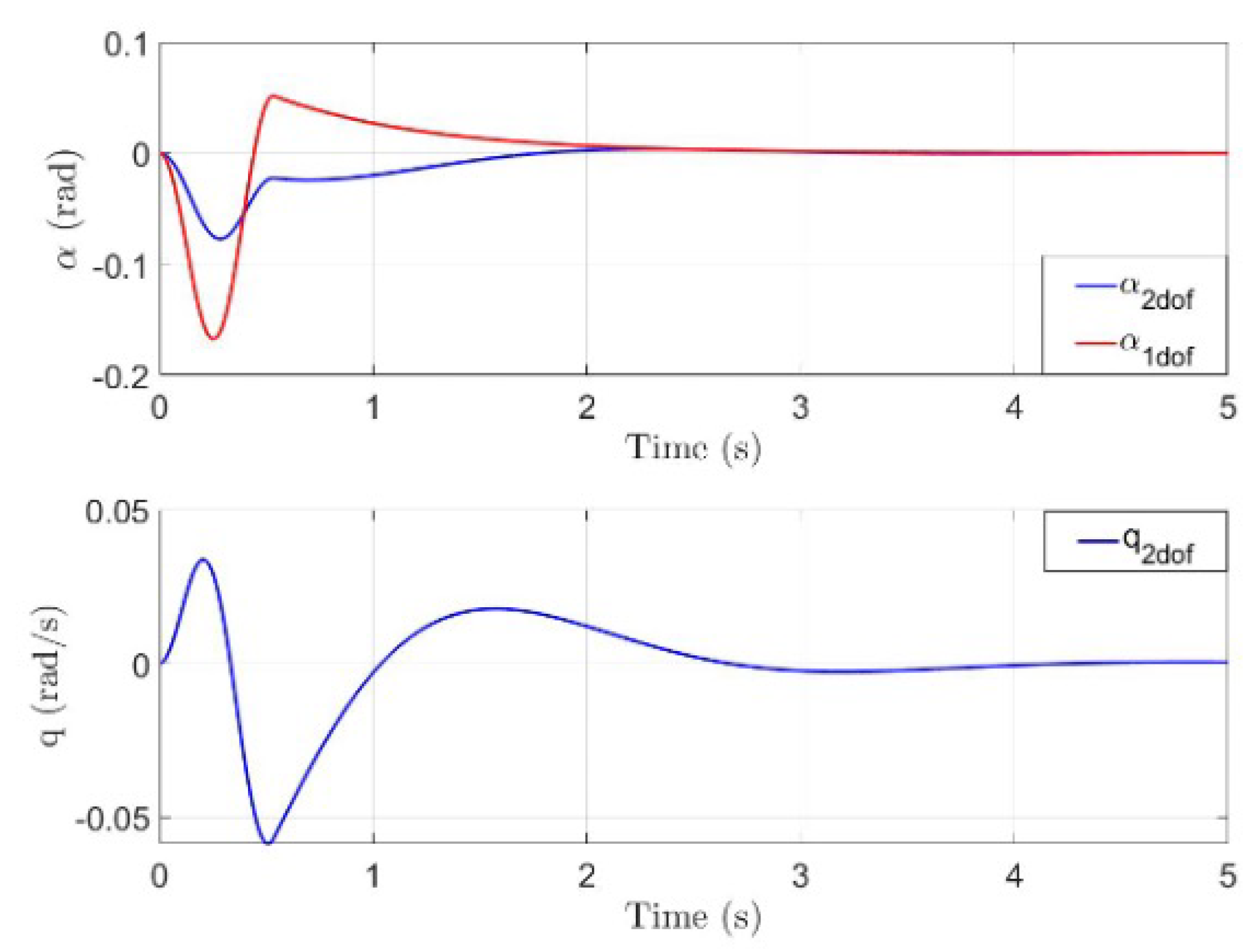
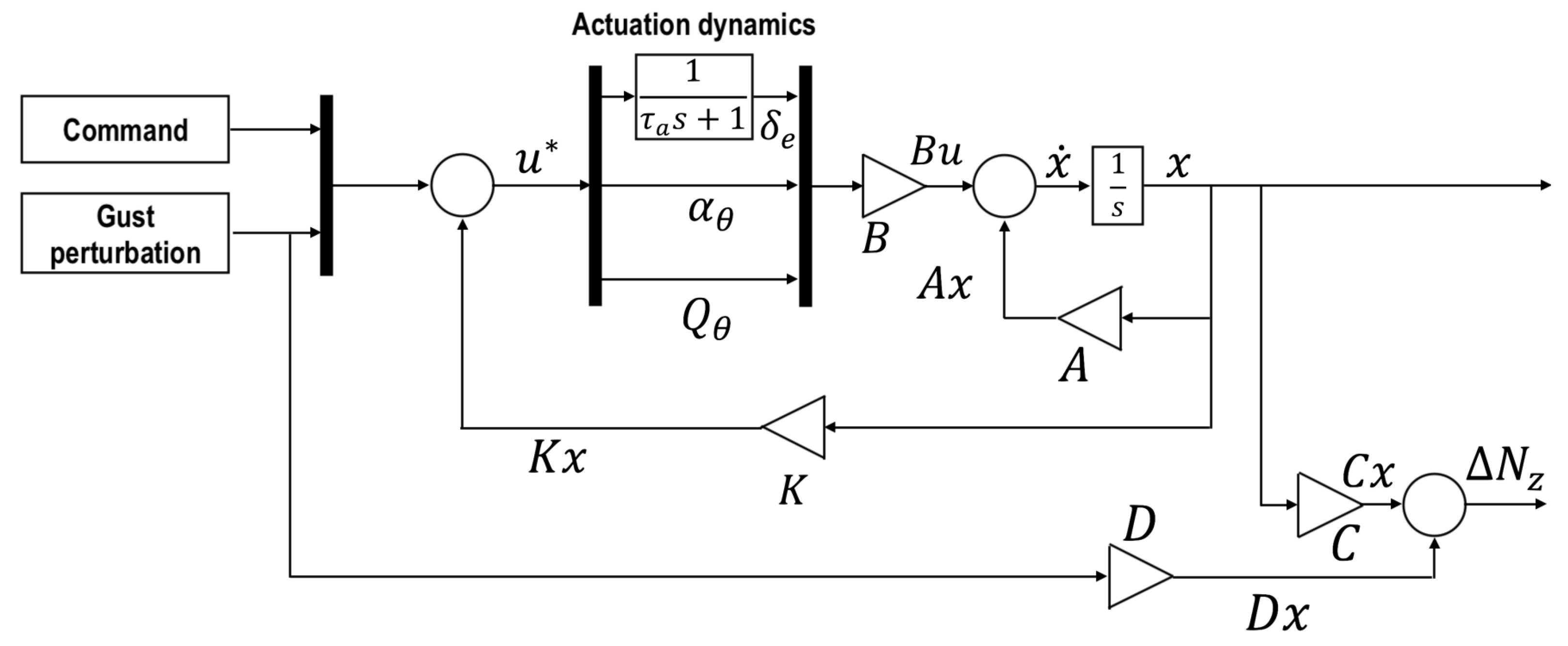
6.2. Aircraft Dynamic Response

Aircraft response to the input described in (39) can be approximated by several methods. For instance, the response to a vertical gust, with a certain magnitude $w_G$, can be estimated considering a pure plunging motion. In terms of a state-space representation, the linear rigid model is approximated by the following equation:

$$\dot{\alpha }=A_{\alpha \alpha }\alpha +A_{\alpha \alpha }{\alpha }_G$$

(40)

Equation (40) is obtained from (36) considering only the angle of attack as a state variable while ${\alpha }_G$, system input, is obtained considering the incidence variation that the vertical gust would induce, see Figure 19a.

The aircraft response in terms of $\mathsf{\Delta }{N}_Z$ to a one-minus-cosine gust with a magnitude of 33 ft/s, producing an ${\alpha }_G$ shown in Figure 19a, with respect to a reference flight condition of straight and level flight with velocity equal to 70 $\mathrm{m}$/$\mathrm{s}$ and an altitude of 1000 $\mathrm{m}$, is reported in Figure 19b. With respect to the reference flight condition, the normal loads factor reached is more than doubled. However, the pure plunging motion approximation is exceedingly conservative, so other models are taken into account.

The load factor response is then evaluated using a dynamic model including two states, for instance the short period mode. As seen in Figure 19b and Figure 20 shows the comparison of the two approximated models with the maximum 2-DoF response being half than the maximum 1-DoF response. The aircraft response to gust input is very fast, thus the short period mode can be assumed as a good approximation of the aircraft dynamics. Again, starting from (36) it is possible to obtain a state-space representation for the short period approximation reported in (41) and (42).

$$\dot{\alpha }=A_{\alpha \alpha }\alpha +A_{\alpha q}q+A_{\alpha \alpha }{\alpha }_G+A_{\alpha q}{Q}_G$$

(41)

$$\dot{q}=A_{q\alpha }\alpha +A_{qq}q+A_{q\alpha }{\alpha }_G+A_{qq}{Q}_G$$

(42)

where $Q_G$ is shown in Figure 21.

The addition of the pitch rate in the state results in a maximum load factor considerably lower with respect to the pure plunge approximation; moreover, the response seems to be smoother. Time histories of the states of the two approximations (pure plunge/short period) are reported in Figure 22. It can be seen that, due to the presence of a pitch angular rate acting out of phase with respect to the angle of attack, there is a reduction in the aircraft response.

Usually, the short period approximation returns a good estimation of the aircraft response to gust. However, due to the high structure flexibility, it is important to investigate the effects of the elastic modes on the full response as well. An approximated flexible model is set up combining the short period approximation with the two elastic modes defined in the previous sections, obtaining a model of dimension six.

The approximated elastic model is triggered with the same gust control input as previously done. The results are reported in Figure 23 and Figure 24, compared with the rigid ones both in terms of $\mathsf{\Delta }{N}_Z$ and states dynamic. It can be seen that a very little difference exists between the responses both in terms of normal loads factor and aircraft states dynamic.

6.3. LQR Design

The LQR is a technique used to design an optimal controller through the minimization of a suitable cost function, representing the states and command energy defined in (43).

$$\left\{\begin{array}{c}{∥u∥}_{R,2}^2={\int }_0^{\infty }{u}^{T}Rudt\hfill \\ {∥x∥}_{Q,2}^2={\int }_0^{\infty }{x}^{T}Qxdt\hfill \end{array}\right.$$

(43)

Matrices R and Q in (43) are symmetric and positive definite. In general, the greater the elements $Q_{ii}$ are, the quicker is the state convergence, at the expense of a larger command. Meanwhile, the greater the elements $R_{ii}$ are, the smaller are the control commands at the expense of a higher states response. Thus, during the design of the control law, a rule of thumb should be to control the feasibility of command actuation, in terms of amplitude and rate of actuation.

The cost function to be minimized by the LQR is defined by the sum of the energy of the states and the energy of the command, as reported in (44).

$$J(x\left(u\right),u)={∥u∥}_{R,2}^2+{∥x∥}_{Q,2}^2={\int }_0^{\infty }\left[x^{T}Qx+u^{T}Ru\right]dt$$

(44)

The solution to the minimization problem of $J\left(x\right(u),u)$ results in a control law characterized by a state feedback as reported in Figure 25 and (45).

$$u^{\ast }=-Kx$$

(45)

Here, K is the matrix of the optimum gains and it is defined as:

$$K=R^{-1}{B}^{T}P$$

(46)

where:

• R is the matrix of weights of the input/command
• B is the control matrix
• P is the solution of the Riccati equation [19]

The stability of the closed loop system is assured by the minimization of the energy related to the states, which guarantees the states convergence. In order to control the aircraft dynamics in the longitudinal plane, only the elevator deflection has been chosen as a control variable, thus the input weight matrix, R, has dimension one.

At the beginning of the analysis, the elevator is supposed to be actuated instantly once the command is given. Then, when the GA will be combined within the LQR controller, a lag, of the form reported in (47), will simulate the actuation dynamics.

$${\displaystyle \frac{{\delta }_e}{u_{act}}}\left(s\right)={\displaystyle \frac{{\tau }_a}{s+{\tau }_a}}$$

(47)

LQR is used to compute the optimal gains, given the weight matrices Q and R, to control the dynamics of the states shown in Figure 25. Moreover, the system reported in (36) is fully controllable and thus the LQR design is feasible.

In the first control design phase, only the rigid states of the flexible model are used as feedback states to control the plant dynamics. Then, supposing to have information about deformation and its time rate of change, the elastic states are used as feedback states as well. In the first case, the states weight matrix Q has dimension $2\times 2$ while in the second one its dimension is $6\times 6$.

It is to be noted that when the LQR is used on its own, Q is chosen as a diagonal matrix, and its coefficient are defined through a trial and error approach. While, when GA and LQR are combined, Q is supposed fully populated and its form is defined by the outcome of the genetic algorithm.

6.3.1. LQR Designed on Rigid States

In the first design loop, only the rigid states ($\alpha$ e q) are used in the feedback controller to control the flexible model dynamics. As previously mentioned, the matrix R has dimension one while the matrix Q has dimension $2\times 2$. Moreover, Q is chosen diagonal with elements $Q_{ii}$ equal to one as for $R_{11}$.

The response of the closed-loop system, reported in red and referred to as $\mathsf{\Delta }N{z}_{fle{x}_{AGRigidStates}}$ in Figure 26, shows a peak smaller than the open-loop system, reported in blue and referred to as $\mathsf{\Delta }N{z}_{flex}$, with less oscillation along the zero value. Meanwhile, in Figure 27, the dynamics of the states is reported showing a more rapid convergence of the rigid states of the closed-loop system, in red, with respect to the open-loop ones, in blue. For the elastic states, the differences are minimal since they are not taken into account in the control design. The command activity required to control the aircraft is reported in Figure 28, showing a quite low but fast command activity.

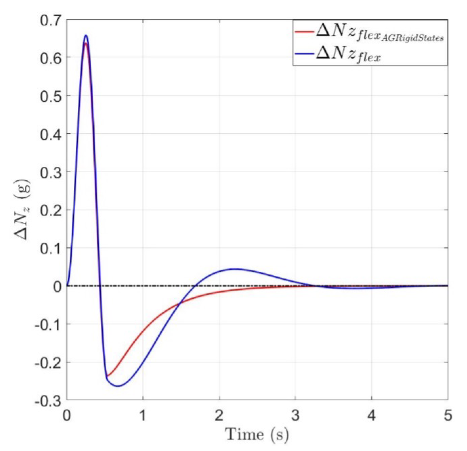
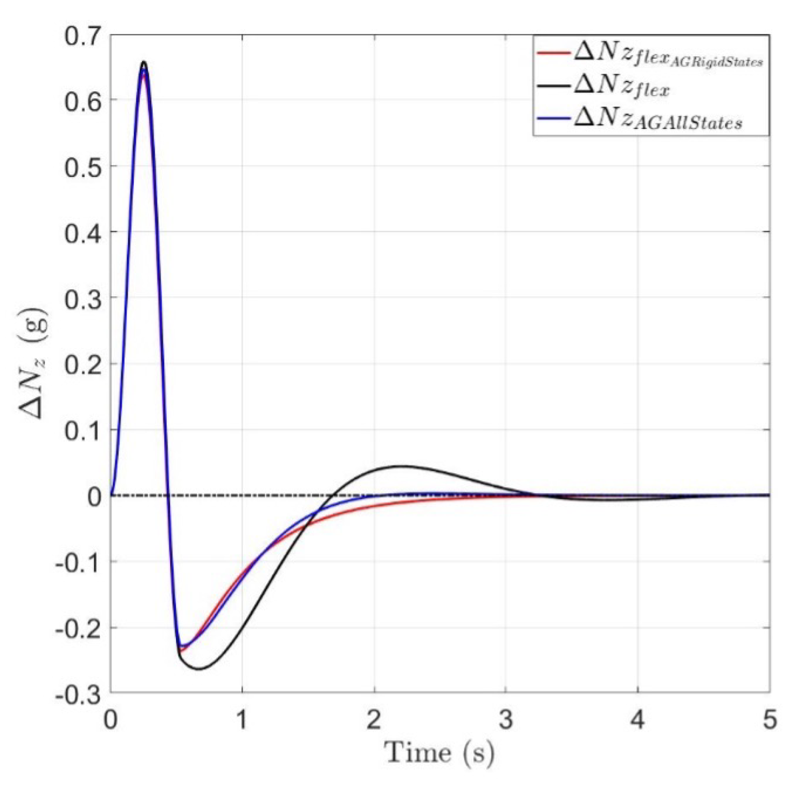
6.3.2. LQR Designed on Elastic States

In a second phase, the LQR is designed considering as feedback states all the model states and thus the matrix Q has dimension $6\times 6$, while the dimension of the matrix R is again one. The results are shown in Figure 29 and Figure 30, showing that the differences between the closed-loop designed with all the states, blue line, and the one designed only with rigid states, red line, are minimal both in terms of normal loads factor and states dynamics.

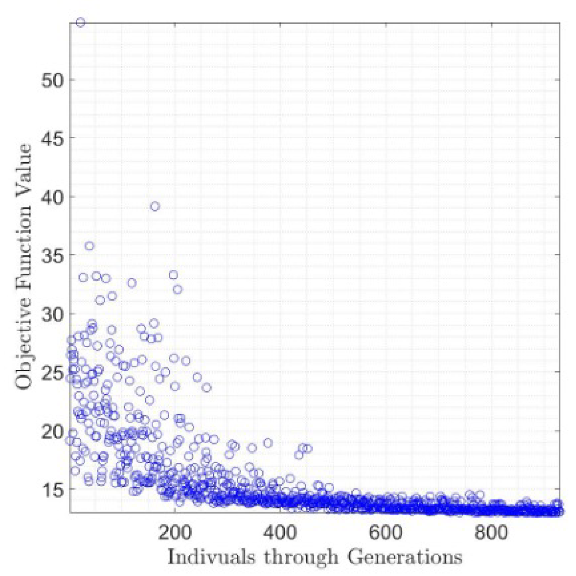
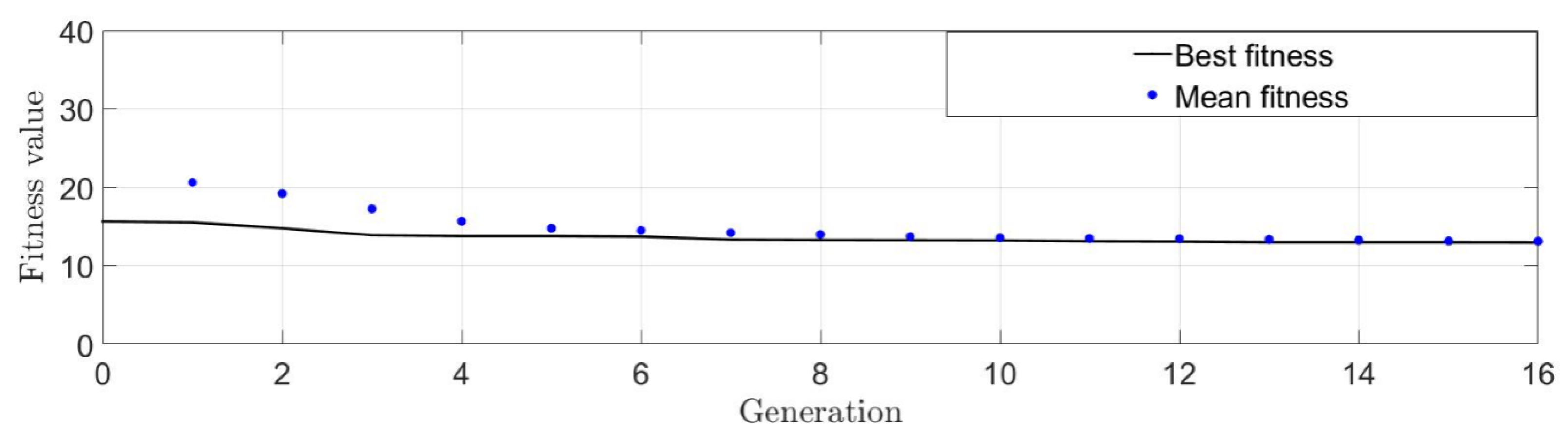
6.4. Genetic Algorithm Application

Coefficients of the Q and R matrices utilised in the LQR controller are usually defined using a trial and error approach, i.e., trying to tune the dynamic response and assuring a feasible command activity. Here, a genetic algorithm is used to determine $Q_{ii}$ and $R_{11}$.

Genetic algorithms are part of the evolutionary and heuristic algorithms and they are usually involved in non-linear and non-smooth optimization problem resolution, minimizing an objective function subject to constraints [18].

Common phases among the several branches of the genetic algorithm are:

• Definition of an initial population (representing an initial set of values for the decision variables)
• Evaluation of the objective/fitness function
• Genetic crossover
• Genetic mutation
• Genetic selection
• Selection of the best genes

While the first and the last step are performed only once, the other ones are repeated until a stopping criterion is reached.

The GA used in this work is developed in MATLAB R2025a and the objective function to be minimised is given by the sum of the energy of $\mathsf{\Delta }{N}_z$ and the energy of the command activity $\mathsf{\Delta }{\delta }_e$, with units weights, as reported in (48).

$$f_{obj}=f(\mathsf{\Delta }{N}_z,\mathsf{\Delta }{\delta }_e)={\int }_{t_0}^{\infty }\left({∥\mathsf{\Delta }{N}_z∥}_{1,2}^2+{∥\mathsf{\Delta }{\delta }_e∥}_{1,2}^2\right)dt$$

(48)

The most relevant options chosen for the GA are reported in

Table 4. GA options.

Option	Value
Population Size	30
EliteCount	0.1 × (Population Size)
SelectionFcn	Stochastic Uniform
CrossoverFcn	Scattered
MutationFcn	AdaptFeasible
Number of Generations	20
Stall Generations (stopping criteria)	15
TolFun (stopping criteria)	0.0001

.

Q and R need to be symmetric and positive-definite: these are the constraints for the algorithm. Thus, the decision variables should be greater than 0 and should satisfy some symmetry conditions. Moreover, weights are introduced to aid in the convergence of the algorithm; the effect of $Q_{ij}$, with i and j rigid DoF, is of two orders of magnitude greater than $Q_{ik}$, with k equal to the flexible state (${\eta }_k$, $k=1,\dots ,n$), and of three orders of magnitude greater than $Q_{im}$ with m equal to the rate of change of the flexible states (${\dot{\eta }}_m$, $m=1,\dots ,n$).

The Simulink scheme of the closed-loop system is shown in Figure 31. A block called Actuation Lag represtns the actuation dynamics as a first order system [16]. The closed-loop system is characterized by states feedback multiplying an optimal gain matrix obtained using a LQR logic with Q and R matrices determined by the GA. Again, inputs to the system are gust perturbations (${\alpha }_G$ and $Q_G$ deriving from a one-minus-cosine gust with amplitude of 33 ft/s) while the command input $\mathsf{\Delta }{\delta }_e$ is regulated by the control law.

Figure 32 shows the values of the objective function through the several populations of different generations. After the first few generations, for which the value of the objective function is between 40 and 15, a horizontal asymptote is reached, as seen in Figure 33.

Figure 33 shows how the mean value of the fitness function after few generations is able to reach the best value. The responses obtained with the optimal gains are the ones shown in Figure 34, Figure 35 and Figure 36, compared with the previous results.

There are some significant results to be highlighted with the usage of the GA:

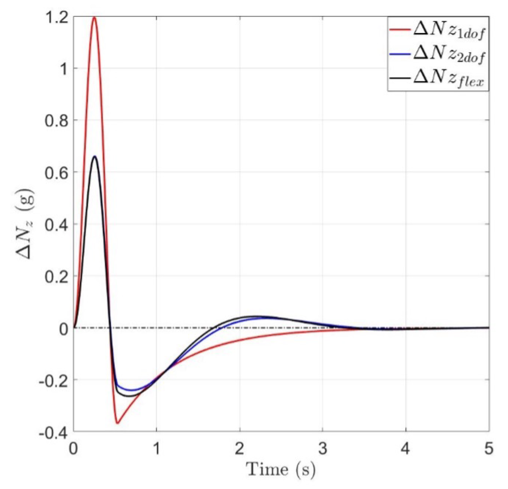
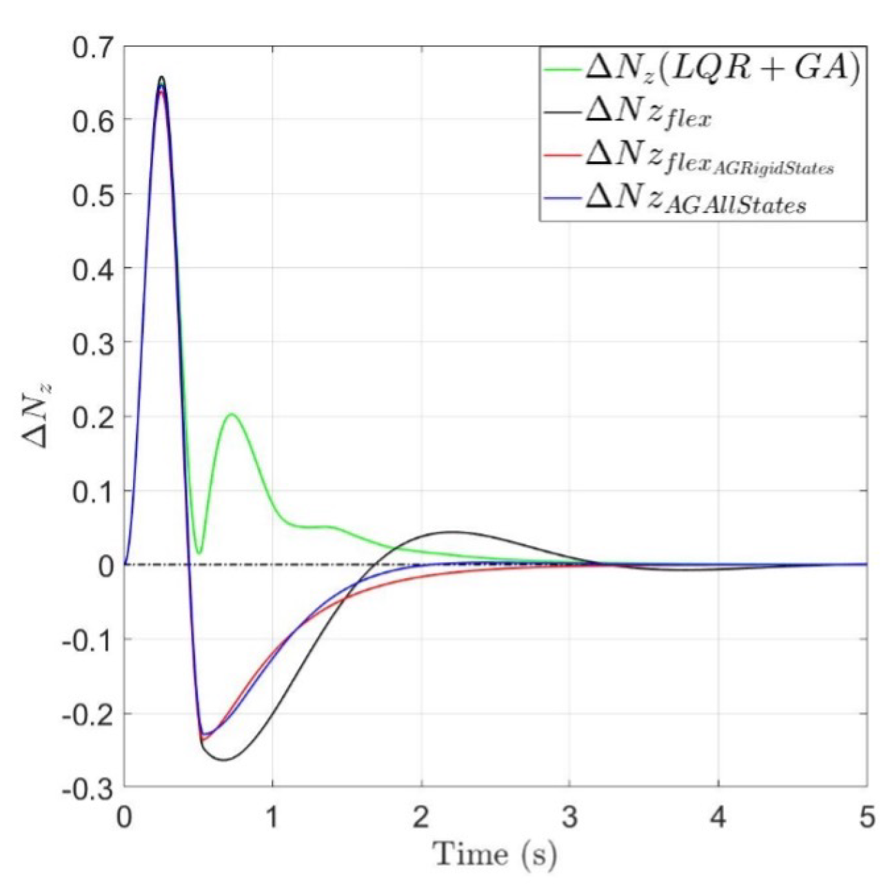
• $\mathsf{\Delta }{N}_z$ obtained with GA application, green line, has a lower energy with respect to the other results. The response does not change sign, but there is still a second oscillation with amplitude 0.2g. The peak response is comparable with the previous one obtained only with LQR
• Rigid state $\alpha$ shows a faster convergence, meanwhile the response in terms of q shows a more oscillating response with greater peak.
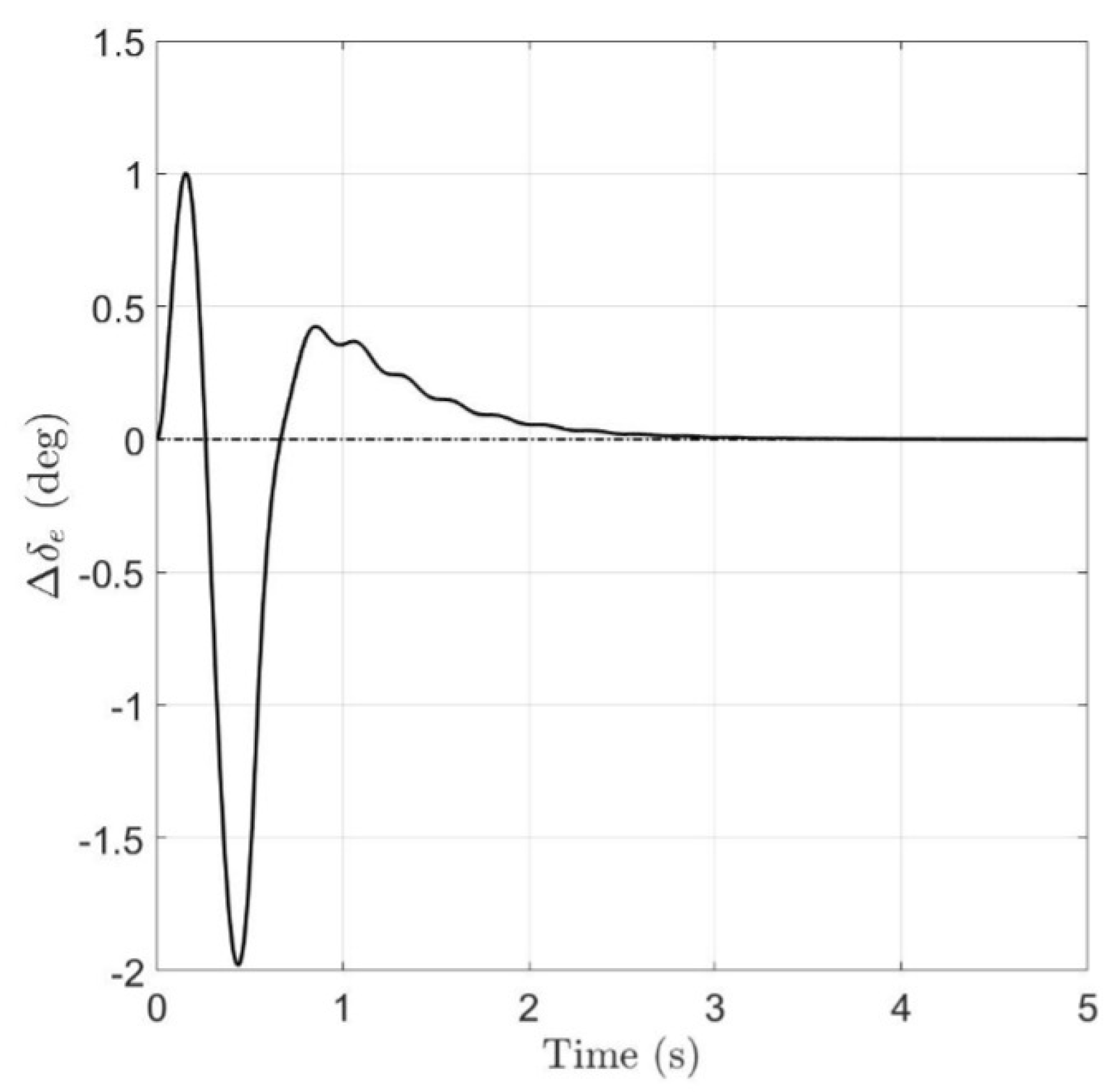
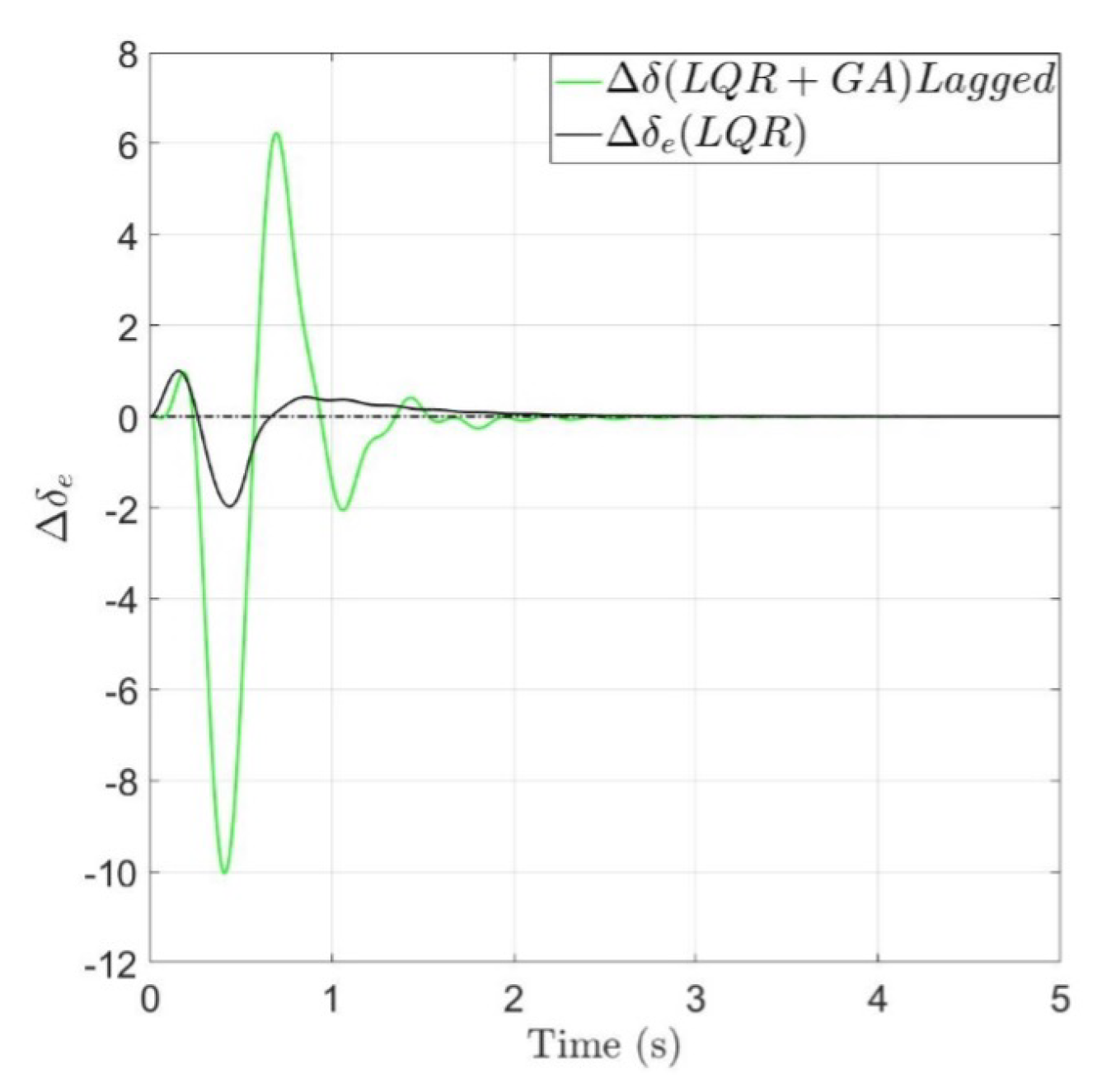
• The command activity required, green line, starts with a certain delay with respect to an instantaneous actuation, black line, due to the actuation dynamics. Peaks are greater and more numerous, however the response in terms of amplitude and actuation time is feasible.

7. Conclusions

Dealing with high aspect ratio aircraft, structural flexibility cannot be neglected in the study of dynamic response, in particular to atmospheric disturb. This work introduces a flexible aircraft longitudinal model derived using the Lagrangian approach. Modal properties are calculated using a FEM analysis with a commercial solver and the aeroelastic derivatives are derived from the 2-D strip theory. As a first step, the difference in the trim conditions between the rigid model and the elastic one are shown. The elastic effects are more significant with increasing velocity. As a second step, the influence of the elastic modes is shown on the rigid body degrees of freedom. This second comparison highlights how a coupling exists between rigid body and structural dynamics. Therefore, the elastic structure plays a significant role in the aircraft dynamics as shown by the present work. The linear elastic model, of reduced dimensions, is useful to tune a suitable controller in the frame of a model-based design approach. The proposed optimal controller, LQR, is designed using a genetic algorithm to define the matrices Q and R and it is tested against a predefined gust input. The use of a flexible aircraft model and the combination of GA and LQR are crucial to define an optimal controller to minimise the vertical acceleration and the elevator displacement.

References

1. Johnston, J.F. Accelerated Development and Flight Evaluation of Active Controls Concepts for Subsonic Transport Aircraft—Volume 1: Load Alleviation/Extended Span Development and Flight Tests; Technical Report NASA-CR159097; NASA: Washington, DC, USA, 1979. [Google Scholar]
2. de Souza Siqueira Versiani, T.; Silvestre, F.J.; Guimarães Neto, A.B.; Rade, D.A.; Annes da Silva, R.G.; Donadon, M.V.; Bertolin, R.M.; Silva, G.C. Gust load alleviation in a flexible smart idealized wing. Aerosp. Sci. Technol. 2019, 86, 762–774. [Google Scholar] [CrossRef]
3. Wright, J.R.; Cooper, J.E. Introduction to Aircraft Aeroelasticity and Loads; Aerospace Series; John Wiley & Sons: Hoboken, NJ, USA, 2008; 488p. [Google Scholar]
4. Jacobson, I.D.; Joshi, D.S. Handling Qualities of Aircraft in the Presence of Simulated Turbulence. J. Aircr. 1978, 15, 254–256. [Google Scholar] [CrossRef]
5. Tsushima, N.; Su, W. A study on adaptive vibration control and energy conversion of highly flexible multifunctional wings. Aerosp. Sci. Technol. 2018, 79, 297–309. [Google Scholar] [CrossRef]
6. Britt, R.; Volk, J.; Dreim, D.; Applewhite, K. Aeroservoelastic Characteristics of the B-2 Bomber and Implications for Future Large Aircraft; Technical Report; Military Aircraft Systems Division, Northrop Grumman Corporation: Pico Rivera, CA, USA, 2000. [Google Scholar]
7. Liu, X.; Sun, Q.; Cooper, J. LQG based model predictive control for gust load alleviation. Aerosp. Sci. Technol. 2017, 71, 499–509. [Google Scholar] [CrossRef]
8. Krag, B.; Rohlf, D.; Wonnenberg, H. OLGA. A Gust Alleviation System for Improvement of Passenger Comfort of General Aviation Aircraft. In Proceedings of the International Council of the Aeronautical Sciences, Munich, Germany, 12–17 October 1980. ICAS-1980-5.4. [Google Scholar]
9. Gao, Z.; Zhu, X.; Fang, Y.; Zhang, H. Active monitoring and vibration control of smart structure aircraft based on FBG sensors and PZT actuators. Aerosp. Sci. Technol. 2017, 63, 101–109. [Google Scholar] [CrossRef]
10. Schmidt, D. Modern Flight Dynamics; McGraw-Hill: New York, NY, USA, 2012. [Google Scholar]
11. Tuzcu, İ. On the stability of flexible aircraft. Aerosp. Sci. Technol. 2008, 12, 376–384. [Google Scholar] [CrossRef]
12. Waszak, M.R.; Schmidt, D.K. Flight dynamics of aeroelastic vehicles. J. Aircr. 1988, 25, 563–571. [Google Scholar] [CrossRef]
13. Schmidt, D.K.; Zhao, W.; Kapania, R.K. Flight-Dynamics and Flutter Modeling and Analyses of a Flexible Flying-Wing Drone—Invited. In Proceedings of the AIAA Atmospheric Flight Mechanics Conference, San Diego, CA, USA, 4–8 January 2016. [Google Scholar] [CrossRef]
14. Schmidt, D. On the integrated control of flexible supersonic transport aircraft. In Proceedings of the Guidance, Navigation, and Control Conference, Baltimore, MD, USA, 7–10 August 1995. [Google Scholar] [CrossRef]
15. Waszak, M.R.; Buttrill, C.S.; Schmidt, D.K. Modeling and Model Simplification of Aeroelastic Vehicles; Technical Report; NASA Langley Research Center: Hampton, VA, USA, 1992. [Google Scholar]
16. Etkin, B.; Reid, L.D. Dynamics of Flight: Stability and Control; Wiley: Hoboken, NJ, USA, 1995. [Google Scholar]
17. Junkins, J.L.; Kim, Y. Introduction to Dynamics and Control of Flexible Structures; AIAA Education Series; AIAA: New York, NY, USA, 1993. [Google Scholar]
18. Nocedal, J.; Wright, S.J. Numerical Optimization, 2nd ed.; Springer Series in Operations Research and Financial Engineering; Springer: New York, NY, USA, 2006. [Google Scholar]
19. Stevens, B.L.; Lewis, F.L. Aircraft Control and Simulation, 2nd ed.; John Wiley & Sons: Hoboken, NJ, USA, 2003. [Google Scholar]
20. Hoblit, F.M. Gust Loads on Aircraft: Concepts and Applications; AIAA: New York, NY, USA, 1988. [Google Scholar]
21. Schmidt, L.V. Introduction to Aircraft Flight Dynamics; AIAA Education Series; AIAA: Reston, VA, USA, 1998. [Google Scholar]
22. United States Department of Defense. MIL-A-8861B: Airplane Strength and Rigidity, Flight Loads; Military Specification; Department of Defense: Washington, DC, USA, 1986. [Google Scholar]
23. European Union Aviation Safety Agency (EASA). Certification Specifications for Normal, Utility, Aerobatic and Commuter Category Aeroplanes (CS-23); Certification specification; EASA: Cologne, Germany, 2010. [Google Scholar]
24. European Union Aviation Safety Agency (EASA). Certification Specifications for Large Aeroplanes (CS-25), Amendment 10; Certification specification; EASA: Cologne, Germany, 2010; Available online: https://www.easa.europa.eu/en/document-library/certification-specifications/cs-25-amendment-10 (accessed on 1 February 2025).
25. Aerodynamic Loads Estimation at Extremes of the Flight Envelope (ALEF). 2012. Available online: https://cordis.europa.eu/project/id/211785/reporting/it (accessed on 1 February 2025).
Figure 1. Modelling approach.
Aerospace 12 00496 g001
Figure 2. Position of the point-mass and representation of the body (solid) and mean axes (dashed) reference frames with positive aerodynamic angles ( α , β ), linear relative velocities (u,v,w) and angular rates (p,q,r).
Aerospace 12 00496 g002
Figure 3. Reference vehicle stick model.
Aerospace 12 00496 g003
Figure 4. Angle of attack, elevator deflection and Power Level Angle setting as a function of velocity for different altitudes.
Aerospace 12 00496 g004
Figure 5. Comparison of natural frequencies ( ω n ) and damping ratios ( ζ ) of the rigid body modes.
Aerospace 12 00496 g005
Figure 6. Argand Diagram for rigid dynamic model. State-space variables: Pitch ( θ ), AoA ( α ), longitudinal speed (u) and pitch rate (q).
Aerospace 12 00496 g006
Figure 7. Vehicle Lumped Model.
Aerospace 12 00496 g007
Figure 8. First elastic mode.
Aerospace 12 00496 g008
Figure 9. Aircraft first elastic mode.
Aerospace 12 00496 g009
Figure 10. Aircraft third elastic mode: first fore and aft wing bending.
Aerospace 12 00496 g010
Figure 11. Third elastic mode.
Aerospace 12 00496 g011
Figure 12. Airfoil elastic motion.
Aerospace 12 00496 g012
Figure 13. Argand Diagram for elastic dynamic model.
Aerospace 12 00496 g013
Figure 14. Root locus of the elastic model.
Aerospace 12 00496 g014
Figure 15. Variation of natural frequency and damping ratio at sea level altitude; (a) Natural frequency variation; (b) Damping ratio variation.
Aerospace 12 00496 g015
Figure 16. Trim condition for an altitude of 7000 m.
Aerospace 12 00496 g016
Figure 17. Gust dynamics process.
Aerospace 12 00496 g017
Figure 18. Aircraft encountering a vertical gust: w G ( x ) vertical velocity profile, w G maximum gust intensity, d gradient distance.
Aerospace 12 00496 g018
Figure 19. Aircraft response to a one minus cosine gust: pure plunging motion approximation. (a) α g ; (b) Δ N z .
Aerospace 12 00496 g019
Figure 20. Effect of degrees of freedom on gust response.
Aerospace 12 00496 g020
Figure 21. Q G due to a one minus cosine gust.
Aerospace 12 00496 g021
Figure 22. Comparison of rigid states dynamic to gust.
Aerospace 12 00496 g022
Figure 23. Effect of elastic degrees of freedom on aircraft response.
Aerospace 12 00496 g023
Figure 24. Comparison of elastic states dynamics.
Aerospace 12 00496 g024
Figure 25. Closed loop system.
Aerospace 12 00496 g025
Figure 26. Effect of a rigid LQR controller on Δ N z .
Aerospace 12 00496 g026
Figure 27. Comparison between closed loop and open loop system.
Aerospace 12 00496 g027
Figure 28. Command activity required.
Aerospace 12 00496 g028
Figure 29. Effect of different LQR controllers on Δ N z .
Aerospace 12 00496 g029
Figure 30. Effect of different LQR controllers on states synamics.
Aerospace 12 00496 g030
Figure 31. Simulink scheme of the controller.
Aerospace 12 00496 g031
Figure 32. Objective functions trend throughout generations.
Aerospace 12 00496 g032
Figure 33. Comparison of best and mean fitness value through generations.
Aerospace 12 00496 g033
Figure 34. Effect of combining LQR and GA controller on Δ N z .
Aerospace 12 00496 g034
Figure 35. Effect of combining LQR and GA controller on aircraft states dynamics.
Aerospace 12 00496 g035
Figure 36. Effect of combining LQR and GA on command activity.
Aerospace 12 00496 g036