Predefined-Time Robust Control for a Suspension-Based Gravity Offloading System ^†

Abstract

Simulating low- or zero-gravity environments on the ground is an important technology in the field of space exploration. Suspension-based gravity offloading (SGO) systems are commonly used ground-based platforms for simulating space environments. Nevertheless, the control of SGO systems presents significant challenges due to external disturbances and stringent response time requirements. This study proposes a predefined-time (PdT) observer-based PdT control framework to address the SGO system control problem. To begin, a pneumatic artificial muscle-based active unloading mechanism is introduced to address the inherent underactuation problem in the SGO system. Thereafter, a PdT disturbance observer is introduced to estimate the external disturbances acting on the SGO system. Subsequently, a type of PdT controller is investigated for the SGO system. The system, including the PdT disturbance observer and the PdT controller, is proven to be PdT stable in the Lyapunov sense. Finally, sufficient numerical simulations and physical experiments are conducted to verify the superiority and effectiveness of the proposed control method.

1. Introduction

Low- and zero-gravity simulation technologies play a vital role in supporting missions such as space exploration, planetary surface sampling, and spacecraft landing [1,2,3]. Gravity offloading systems are indispensable for simulating the gravitational environments encountered in space or on extraterrestrial bodies [4,5]. Various microgravity simulation platforms have been developed based on different physical principles. Mechanically based systems such as drop towers and catapult mechanisms offer brief periods of true free-fall conditions, but their short duration and infrastructure requirements limit their practicality [6,7]. In contrast, emerging magnetic levitation platforms [8,9] provide contactless and controllable environments, though they are constrained by limited payload capacity and challenges in maintaining magnetic field uniformity. Compared to these approaches, gravity offloading systems—especially suspension-based gravity offloading (SGO) systems—have become the most widely used solution for terrestrial simulation of low-gravity environments. SGO systems are relatively easy to deploy, compatible with a wide range of payloads, and capable of supporting continuous low-gravity testing. They have been extensively employed in ground testing of spacecraft and astronaut training, serving as a key enabling technology for mission validation and performance assessment [10]. As illustrated in Figure 1, an SGO system typically consists of a two-axis tracking mechanism and a suspension structure designed to simulate reduced-gravity environments.

Despite their practical utility, achieving precise control of SGO systems remains a significant challenge. The primary control challenges stem from underactuation, unmodeled characteristics [11,12], and disturbances caused by low structural rigidity [13] or highly flexible suspended objects [14]. In recent years, various robust control strategies have been developed to address modeling uncertainties and unknown disturbances, including nonlinear disturbance estimation [15], RBF-based predictive control [16], and fuzzy uncertainty observers [17].

However, the aforementioned methods typically rely on prior knowledge of disturbance bounds and precise system modeling. In addition, they generally do not provide guarantees on convergence within a finite or predefined time frame. Such limitations significantly hinder their application to SGO systems, which demand high real-time responsiveness and strong robustness to disturbances. Consequently, developing a control strategy that ensures both robust performance and guaranteed convergence time remains an urgent and challenging task. In response, recent efforts have focused on advanced control strategies such as sliding mode control [18], adaptive finite-time control [19], and neural network-based approaches [20]. In [21], a fast finite-time robust adaptive terminal sliding mode controller was proposed for nonlinear systems with uncertainties and unmodeled dynamics. This method ensures finite-time stability and enables the system output to rapidly converge to its desired trajectory. An adaptive backstepping-based finite-time control approach was proposed in [22] for a class of feedback nonlinear systems subject to unmodeled dynamics and unknown external disturbances. Considering the presence of unknown stochastic disturbances, traditional fast finite-time control methods become inapplicable. To address this issue, Wang et al. [23] proposed a neural network-based fast finite-time control strategy by constructing an auxiliary function and leveraging Jensen’s inequality.

Although the aforementioned methods provide convergence time guarantees and robustness [24], the convergence time in finite-time control schemes typically depends on the system’s initial conditions [25]. As such, when the initial tracking error is large, the resulting convergence time may still fail to meet practical performance requirements [26,27,28]. This limitation is particularly problematic in SGO systems, where it is crucial to complete control tasks within a guaranteed time frame—especially during landing simulations under low-gravity conditions, to ensure system stability, safety, and environmental fidelity. To overcome this limitation, predefined-time (PdT) control has emerged as a research hotspot and has been applied in nonlinear systems such as spacecraft [29] and robotic platforms [30]. In [31], an adaptive predefined-time tracking controller was proposed to address unmodeled dynamics in the system, guaranteeing that the tracking error converges to a small neighborhood around zero within a predefined time. Wang et al. [32] proposed an adaptive fuzzy PdT control method for uncertain strict-feedback nonlinear systems, ensuring the tracking error converges to an arbitrarily small neighborhood of the origin. Considering a class of general uncertain distributed-order dynamical systems, Muñoz-Vázquez et al. [33] proposed a predefined-time sliding mode design that enforces predefined-time convergence of the system trajectories.

While PdT control strategies have demonstrated promising results, their standalone application may be insufficient for systems such as SGO that are subject to unmodeled dynamics and external disturbances. To enhance disturbance rejection capabilities, several recent studies have explored the integration of PdT controllers with disturbance observers. For example, Sun et al. [34] proposed a PdT sliding mode control method that incorporates a nonlinear disturbance observer. In [35], a predefined-time sliding mode controller was developed for an n-dimensional chaotic system with disturbances and uncertainties, using a disturbance observer to estimate the composite disturbance. Ji et al. [36] combined predefined-time sliding mode control with a finite-time disturbance observer to address modeling inaccuracies and parameter perturbations in long-stator linear synchronous motors. However, most of these methods ensure PdT convergence only within a local region of the state space. To achieve global PdT stability in the presence of unmodeled dynamics and external disturbances, it is essential to design a corresponding PdT disturbance observer (PdTDO) capable of accurately estimating unknown disturbances within a predefined time.

Motivated by the above analysis, this paper aims to develop a PdT robust controller (PdTRC) with a PdT observer for low-gravity offloading systems subject to unmodeled dynamics and unknown disturbances. These unknown disturbances include oscillatory tension variations in cables, vibration induced by flexible suspended components, and actuator friction and backlash. The main contributions of this work are summarized as follows:

(1)

A PdT observer is developed to estimate unmodeled dynamics and unknown external disturbances. In contrast to the methods proposed in [37,38], the observation error in the proposed approach converges to a smaller neighborhood within a predefined time.

(2)

A predefined-time robust controller integrated with a predefined-time observer is proposed to address unmodeled dynamics and unknown disturbances in SGO systems. Compared with the methods presented in [33,39], the proposed approach can effectively guarantee predefined-time convergence of the SGO system.

(3)

A pneumatic artificial muscle (PAM) structure is introduced to address the underactuation and control bandwidth limitation issues arising from the use of passive springs for impact disturbance attenuation in traditional SGO systems. Finally, the effectiveness and superiority of the proposed control framework are validated through extensive simulations and physical experiments.

The remainder of this paper is organized as follows. Section 2 introduces the SGO system platform, establishes the dynamic model of the suspension constant force (SCF) subsystem, and highlights the key problems addressed in this study. In Section 3, a predefined-time observer is designed, and predefined-time controllers are respectively developed for the descent phase and the landing buffering phase. Section 4 presents numerical simulations to evaluate the performance of the proposed control strategy under various disturbance scenarios. Section 5 provides physical experiments conducted on the SGO platform to further validate the effectiveness and robustness of the proposed approach in real-world conditions. Finally, Section 6 summarizes the main findings and concludes the paper.

In what follows, for convenience and clarity, some commonly used variables are defined as follows: $J_r$ is the moment of inertia of the reducer input shaft. $J_m$ is the moment of inertia of the motor rotor. $\omega$ represents the angular velocity at the reducer output. n is the gear reduction ratio. ${\tau }_m$ is the electromagnetic torque generated by the motor while ${\tau }_l$ is the load torque. $c_r$ represents the rotational damping coefficient, r is the radius of the pulley, and $F_l$ is the force transmitted to the load. $m_c$ and $m_p$ denote the equivalent mass of the cable and the PAM, respectively. ${\ddot{x}}_1$ is the acceleration at the load-side pulley point. $f_y(x_p,{\dot{x}}_p,u)$ is the nonlinear force generated by the PAM. $d_l$ is the bounded unknown external disturbance. $x_3$ is the compressive displacement during the landing buffering phase. ${\dot{x}}_3$ is the compression velocity during the landing buffering phase. $k_l$ and $c_l$ represent the unknown stiffness coefficient of the elastic support and the unknown damping coefficient of the elastic support, respectively. $m_l$ and $m_s$ are the mass of the load and the force sensor, respectively. g is the gravitational acceleration, and ${\ddot{x}}_2$ is the vertical acceleration of the load.

2. System Modeling

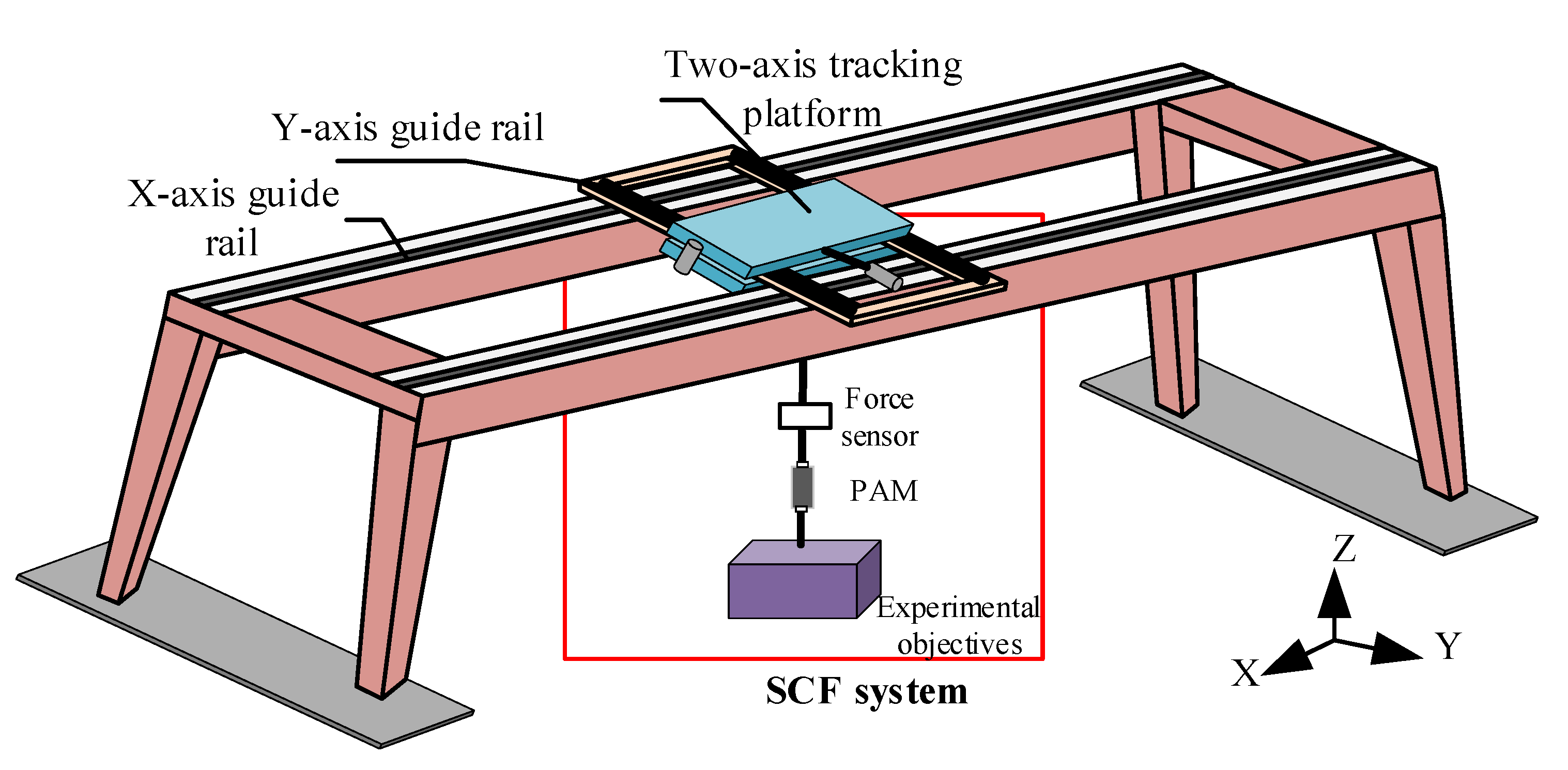
2.1. Suspension Gravity Offload Platform

As depicted in Figure 1, the SGO system with beam structures is an efficient gravity offloading technique. The SGO consists of a two-dimensional tracking subsystem responsible for achieving horizontal movement and an SCF subsystem utilized to apply a counterforce to the experimental target through suspension without breaking the stability of the system. To mitigate force impact and reduce cable tension errors, passive dampers are incorporated. However, the bandwidth and the accuracy of the system would decrease due to the underactuation problem caused by the passive dampers.

Focusing on the SCF subsystem within the SGO system. Figure 2 illustrates the schematic diagram of the SCF subsystem based on the PAM proposed in this study.

As shown in Figure 2, the SCF system consists of a torque motor and a PAM. The torque motor, coupled with a reducer, regulates the spatial position within the load space, while the PAM replaces traditional passive dampers and directly maintains constant force control with the load. In addition, the SCF system integrates laser displacement sensors and force sensors for state feedback. In Figure 2, $x_1$ represents the displacement of the pulley, $x_p=x_{p0}+(x_1-x_2)$ denotes the length of the PAM, $x_2$ indicates the displacement of the load. In landing buffering experiments of spacecraft under micro/low-gravity conditions, $x_3$ represents the compression displacement during the touchdown buffering phase. The motion direction of the entire SCF system is defined such that upward motion is positive and downward motion is negative.

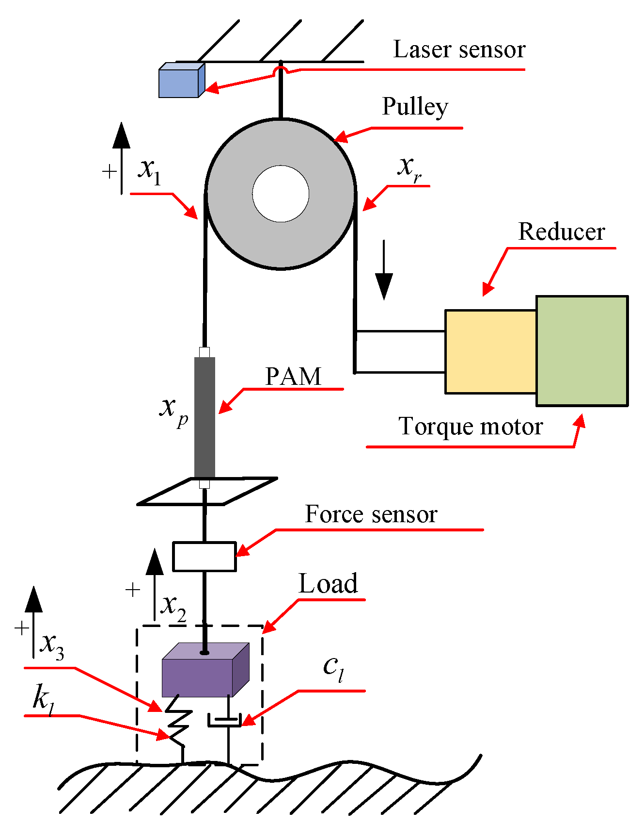
2.2. Mathematical Model of SCF

Figure 2 illustrates the structure of the SCF system, which is developed to simulate low-gravity environments by applying controllable offloading forces to a suspended load through multi-source actuation. The SCF system integrates a torque motor and a PAM, forming a typical multi-input single-output (MISO) actuation architecture. From a dynamic perspective, the landing process in low-gravity environments can be segmented into two distinct phases: (1) the descent phase, where the suspended payload undergoes accelerated motion under reduced gravity; and (2) the landing buffering phase, which begins once the load contacts the elastic support, during which impact forces are attenuated and kinetic energy is dissipated.

The complete dynamic model of the SCF system is given by

$$(J_r+J_m)n^2\dot{\omega }=n{\tau }_m-{\tau }_l-c_r\omega ,$$

(1)

$$F_l={\displaystyle \frac{{\tau }_l}{r}}=(m_c+m_p){\ddot{x}}_1+f_y(x_p,{\dot{x}}_p,u)+d_l,$$

(2)

$$f_y(x_p,{\dot{x}}_p,u)-(k_l{x}_3+c_l{\dot{x}}_3)-(m_l+m_s)g=(m_l+m_s){\ddot{x}}_2,$$

(3)

We further define the linear velocity of the reducer output as ${\dot{x}}_r=R\omega$ to combine the rotational and translational motion, where R denotes the radius of the drum at the reducer end. Similarly, the linear velocity at the pulley end is given by ${\dot{x}}_1=r{\omega }_1$ with ${\omega }_1$ being the angular velocity of the pulley. Assuming ideal transmission (i.e., negligible pulley deformation and slippage) yields ${\dot{x}}_1\approx {\dot{x}}_r$, yielding

$${\dot{x}}_1=R\omega ,\mathrm{and}{\ddot{x}}_1=R\dot{\omega }.$$

Substituting ${\ddot{x}}_1=R\dot{\omega }$ into (2) yields the expression for the load torque:

$${\tau }_l=(m_c+m_p)rR\dot{\omega }+f_y(x_p,{\dot{x}}_p,u)r+r{d}_l$$

(4)

Finally, by substituting (4) into (1), we have

$$(J_r+J_m)n^2\dot{\omega }+(m_c+m_p)rR\dot{\omega }+c_r\omega =n{\tau }_m-f_y(x_p,{\dot{x}}_p,u)r-r{d}_l$$

(5)

The PAM in the SCF system achieves active cushioning only by adjusting u during the landing buffering phase. Specifically, in the simulated micro-low-gravity descent phase, $k_l=0$ and $c_l=0$, whereas during the landing buffering phase, $k_l\ne 0$ and $c_l\ne 0$. Therefore, the dynamic model of the SCF system (1)–(5) is divided into two parts:

(1) Model Formulation for the Descent Phase

$$\begin{array}{c}\hfill \begin{array}{c}\hfill f_y(x_p,{\dot{x}}_p,u)-(m_l+m_s)g=(m_l+m_s){\ddot{x}}_2\end{array}\end{array}$$

(6)

Under the constant-pressure control of the PAM, the linear velocity during the descent phase satisfies the kinematic relationship ${\dot{x}}_2={\dot{x}}_1=R\omega$. Substituting (6) into (5) yields

$$\begin{array}{c}\hfill \begin{array}{c}\hfill J\dot{\omega }+c_r\omega +(m_l+m_s)gr=\tau +d\end{array}\end{array}$$

(7)

where $J=(J_r+J_m)n^2+(m_c+m_p+m_l+m_s)rR$, $\tau =n{\tau }_m$, and $d=-r{d}_l$.

(2) Model Formulation for the Landing Buffering Phase

$$\begin{array}{cc}\hfill & \begin{array}{c}\hfill J_L\dot{\omega }+c_r\omega =\tau -f_y(x_p,{\dot{x}}_p,u)r+d,\end{array}\hfill \end{array}$$

(8)

$$\begin{array}{cc}\hfill & \begin{array}{c}\hfill f_y(x_p,{\dot{x}}_p,u)-(k_l{x}_2+c_l{\dot{x}}_2)-(m_l+m_s)g=(m_l+m_s){\ddot{x}}_2,\end{array}\hfill \end{array}$$

(9)

$$\begin{array}{cc}\hfill & \begin{array}{c}\hfill F_p=f_y(x_p,{\dot{x}}_p,u)=(f_1+f_{2}u)+\sum _{i=1}^2(b_{i1}+b_{i2}u){\dot{x}}_p^i+\sum _{i=1}^2(k_{i1}+k_{i2}u)x_p^i,\end{array}\hfill \end{array}$$

(10)

where $J_L=(J_r+J_m)n^2+(m_c+m_p)rR$ denotes the lumped rotational inertia reflected to the motor side. The coefficients $f_1$ and $f_2$ represent the static force components in the PAM model. The parameters $b_{i1}$ and $b_{i2}$ correspond to the velocity-dependent damping terms, while $k_{i1}$ and $k_{i2}$ are associated with position-dependent stiffness effects. All parameters were experimentally identified, as detailed in [40]. The variable u denotes the control input applied to the PAM.

The nonlinear function $f_y(x_p,{\dot{x}}_p,u)$ is linearized using a first-order Taylor series expansion around the operating point, where higher-order terms are neglected to obtain a linear approximation suitable for system analysis and control design. This method transforms the original nonlinear system into a linearized model expressed as follows:

$$\begin{array}{c}\hfill \begin{array}{c}\hfill F_p=f_y(x_p,{\dot{x}}_p,u)\approx f_{p0}+K_a\Delta x_p+K_b\Delta {\dot{x}}_p+K_c\Delta u\end{array}\end{array}$$

(11)

where

$$\begin{array}{cc}\hfill f_{p0}& =f_y{|}_{(x_{p0},{\dot{x}}_{p0},u_0)},\hfill \\ \hfill K_a& ={\displaystyle \frac{\partial f_y}{\partial x_p}}=\sum _{i=1}^{2}i·(k_{i1}+k_{i2}{u}_0)x_{p0}^{i-1},\hfill \\ \hfill K_b& ={\displaystyle \frac{\partial f_y}{\partial {\dot{x}}_p}}=\sum _{i=1}^{2}i·(b_{i1}+b_{i2}{u}_0){\dot{x}}_{p0}^{i-1},\hfill \\ \hfill K_c& ={\displaystyle \frac{\partial f_y}{\partial u}}=f_y+\sum _{i=1}^2{b}_{i2}{\dot{x}}_{p0}^i+\sum _{i=1}^2{k}_{i2}{x}_{p0}^i.\hfill \end{array}$$

2.3. Control Objective

Based on the analysis aforementioned and the assumptions, the control objectives of this study are formulated as follows.

(1) Descent Phase: For a set of expected acceleration $a_r$, design a type of PdT controller for the load of the SGO system such that

$$\begin{array}{c}\hfill \underset{t\to T_p}{lim}\left({\ddot{x}}_1-a_r\right)=0\end{array}$$

where ${\ddot{x}}_1$ denotes the vertical acceleration of the load, $a_r$ is the desired reference acceleration, and $T_p>0$ is the predefined time.

(2) Landing Buffering Phase: For a set of desired force $F_s$, design a type of PdT controller such that

$$\begin{array}{c}\hfill \underset{t\to T_d}{lim}max\left(\right|{\dot{x}}_1|,|{\dot{x}}_2\left|\right)\le {ϵ}_v,\underset{t\to T_d}{lim}|F_p-F_s|\le {ϵ}_F\end{array}$$

where ${\dot{x}}_1$ and ${\dot{x}}_2$ denote the velocities of the motor-driven pulley system and the suspended load, respectively; constants ${ϵ}_v,{ϵ}_F>0$ specify the allowable upper bound of the residual velocity and the force, and $T_d>0$ is the predefined time.

Remark 1. 

For control objective 1, to achieve this acceleration, the SCF system must provide a vertical upward offloading force $F_r$ that partially counteracts gravity.

$$\begin{array}{c}\hfill F_r=m(g-a_r),\end{array}$$

where $F_r$ denotes the upward support force applied by the SCF system, $m=m_c+m_p+m_l+m_s$ is the total suspended mass, and g is the gravitational acceleration.

For control objective 2, the expected force $F_s$ can be given by $F_s=(m_l+m_s)(g-a_r)$. The allowable residual velocity and force bounds are denoted as ${ϵ}_v$ and ${ϵ}_F$, respectively, whose specific values are discussed in the simulation section.

3. Predefined-Time Control and Observer Design 

3.1. Predefined Time Convergence Criteria

Definition 1 

([41,42]). Consider the continuous-time nonlinear system

$$\begin{array}{c}\hfill \begin{array}{c}\hfill \dot{x}=f(x,t)\end{array}\end{array}$$

(12)

where $x\in {\mathbb{R}}^n$ is the system state, $f(·)$ is a possibly non-Lipschitz function satisfying $f(0,t)=0$, and $x\left(0\right)=x_0$. If there exists a predefined time $T_c>0$ such that the solution $x(t,x_0)$ of system (12) satisfies $x\left(t\right)=0$ for all $t\ge T_c$ and for all $x_0\in {\mathbb{R}}^n$, then the equilibrium point of the system (12) is said to be globally predefined time stable, and $T_c$ is called the predefined time. Note that finite-/predefined-time convergence typically requires the system dynamics to be non-Lipschitz near the equilibrium.

Definition 2 

([43]). The origin of system (12) is said to be globally practically predefined-time stable if there exist constants $\eta >0$ and $T_c>0$ such that the solution $x(t,x_0)$ satisfies

$$\begin{array}{c}\hfill \parallel x(t,x_0)\parallel \le \eta ,\forall t\ge T_c,\forall x_0\in {\mathbb{R}}^n.\end{array}$$

In this case, the trajectory of the system converges to a residual set of radius η within a predefined time $T_c$.

Lemma 1 

([30]). For system (12), if there exists a radially unbounded positive function $V\left(x\right)$ such that

$$\begin{array}{c}\hfill \begin{array}{c}\hfill \dot{V}\left(x\right)\le -{\displaystyle \frac{\pi }{\delta T_c\sqrt{\alpha \beta }}}\left(\alpha V^{1-{\displaystyle \frac{\delta }{2}}}+\beta V^{1+{\displaystyle \frac{\delta }{2}}}\right),\end{array}\end{array}$$

(13)

where $T_c>0$ is the predefined time, $\delta \in (0,1)$, and $\alpha ,\beta >0$. The origin of system (12) is globally predefined-time stable, and the upper bound of the settling time is $T_c$.

Lemma 2 

([32,44]). Consider system (12). If there exists a radially unbounded positive function $V\left(x\right)$ such that

$$\begin{array}{c}\hfill \begin{array}{c}\hfill \dot{V}\left(x\right)\le -{\displaystyle \frac{\pi }{\delta T_c\sqrt{\alpha \beta }}}\left(\alpha V^{1-{\displaystyle \frac{\delta }{2}}}+\beta V^{1+{\displaystyle \frac{\delta }{2}}}\right)+\eta ,\end{array}\end{array}$$

(14)

where $T_c>0$ is a predefined time, $\delta \in (0,1)$, $\alpha ,\beta >0$, and $\eta >0$. Then the solution $x\left(t\right)$ converges to a residual set within the predefined time $T_{pc}=T_c/\sqrt{\mu }$, where $0<\mu <1$, and the residual set is given by

$$\begin{array}{c}\hfill \begin{array}{c}\hfill \left\{x\in {\mathbb{R}}^n|V\left(x\right)\le min\left\{{\left({\displaystyle \frac{\eta \delta T_c\sqrt{\alpha \beta }}{\pi \alpha (1-\mu )}}\right)}^{{\displaystyle \frac{2}{2-\delta }}},{\left({\displaystyle \frac{\eta \delta T_c\sqrt{\alpha \beta }}{\pi \beta (1-\mu )}}\right)}^{{\displaystyle \frac{2}{2+\delta }}}\right\}\right\}.\end{array}\end{array}$$

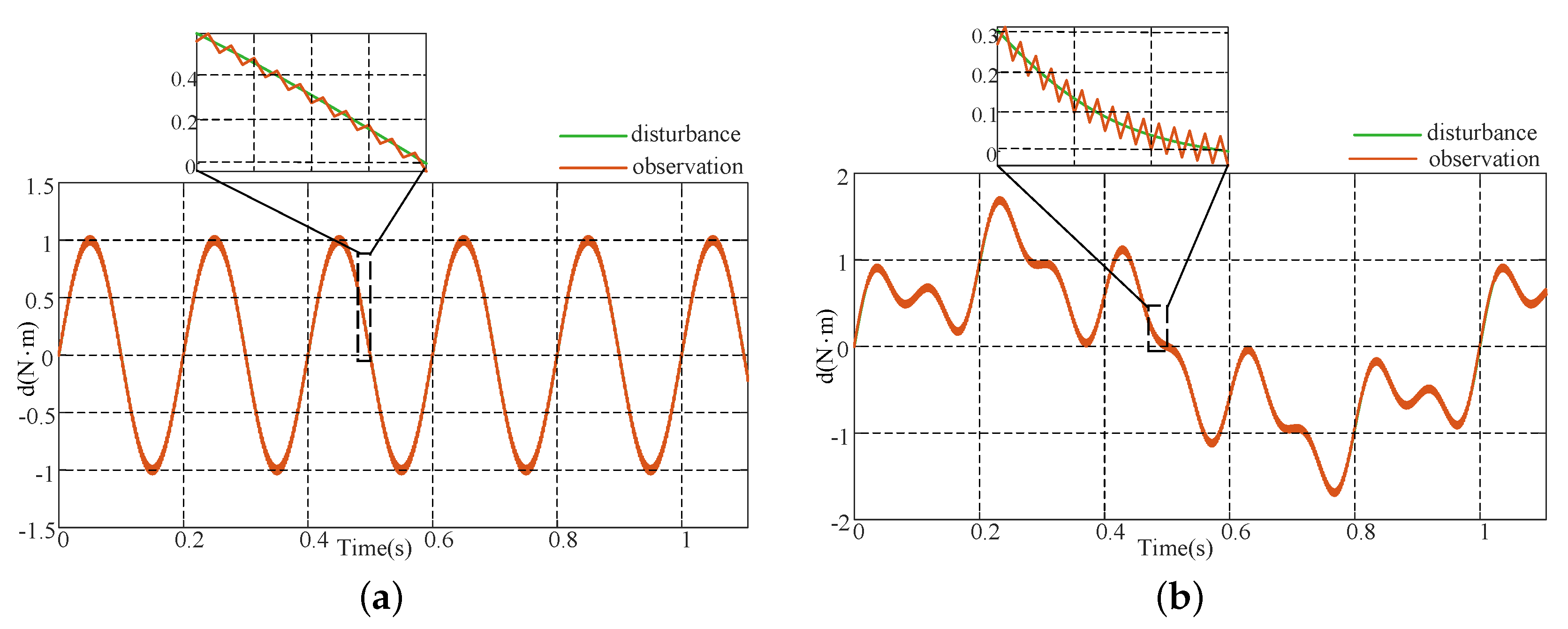
3.2. Predefined-Time Disturbance Observer Design

For working scenarios with uncertainties and disturbances, a disturbance observer is an essential component in control system design. In this study, the PdTDO is proposed as follows:

$$\begin{array}{c}\hfill \begin{array}{cc}\hfill \dot{\widehat{d}}& =-{\displaystyle \frac{\pi }{2{\delta }_o{T}_o}}\left({\displaystyle \frac{1}{\sqrt{{ϵ}_o}}}+\sqrt{{ϵ}_o}\right){\displaystyle \frac{\widehat{d}-d_{\mathrm{ap}}}{\sqrt{|\widehat{d}-d_{\mathrm{ap}}|}+{ϵ}_o}},\hfill \\ \hfill d_{\mathrm{ap}}& =\overline{J}\dot{\omega }+{\overline{c}}_r\omega +(m_l+m_s)gr-{\tau }_a\hfill \end{array}\end{array}$$

(15)

where $T_o>0$ is the predefined convergence time, ${\delta }_o\in (0,1)$ is a tuning parameter, and ${ϵ}_o\in (0,1)$ is a small regularization constant ensuring continuity. Specifically, $\overline{J}$ and ${\overline{c}}_r$ denote the nominal values of parameters J and $c_r$, respectively, and $\omega$, $\dot{\omega }$, and ${\tau }_a$ are measured angular velocity, angular acceleration, and torque. The PdT stability of the observer is established through the following theorem.

Note that the reference torque ${\tau }_a$ is constrained to lie within a positive bounded range, i.e., ${\tau }_a\in [{\tau }_{min},{\tau }_{max}]$ with ${\tau }_{min}>0$, as the offloading system only applies unidirectional lifting forces.

Assumption A1. 

The estimation error of the disturbance is bounded, namely, $|d_{\mathrm{ap}}-d|\le {\Delta }_d$ for some ${\Delta }_d>0$.

Theorem 1. 

With Assumption A1, the PdTDO in (15) guarantees that the estimation error $\tilde{d}=\widehat{d}-d$ converges into a residual set within the predefined time $T_o$, i.e.,

$$\begin{array}{c}\hfill \underset{t\to T_o}{lim}|\widehat{d}-d|\le {ϵ}_d,\end{array}$$

(16)

where the residual set radius ${ϵ}_d$ is explicitly given by

$$\begin{array}{c}\hfill {ϵ}_d={\left({\displaystyle \frac{{\delta }_o{T}_o{\Delta }_d}{\pi }}\right)}^2+{ϵ}_o.\end{array}$$

Proof. 

Define the estimation error as $\tilde{d}=\widehat{d}-d$, whose dynamics are given by the following:

$$\begin{array}{c}\hfill \dot{\tilde{d}}=-{\displaystyle \frac{\pi }{2{\delta }_o{T}_o}}\left({\displaystyle \frac{1}{\sqrt{{ϵ}_o}}}+\sqrt{{ϵ}_o}\right){\displaystyle \frac{\tilde{d}+(d-d_{\mathrm{ap}})}{\sqrt{|\tilde{d}+(d-d_{\mathrm{ap}})|}+{ϵ}_o}}-\dot{d}.\end{array}$$

Consider the following Lyapunov candidate function:

$$\begin{array}{c}\hfill V\left(t\right)={\displaystyle \frac{1}{2}}{\tilde{d}}^2.\end{array}$$

Taking the derivative of $V\left(t\right)$, we have

$$\begin{array}{c}\hfill \dot{V}\left(t\right)=\tilde{d}\dot{\tilde{d}}=-{\displaystyle \frac{\pi }{2{\delta }_o{T}_o}}\left({\displaystyle \frac{1}{\sqrt{{ϵ}_o}}}+\sqrt{{ϵ}_o}\right){\displaystyle \frac{\tilde{d}\left[\tilde{d}+(d-d_{\mathrm{ap}})\right]}{\sqrt{|\tilde{d}+(d-d_{\mathrm{ap}})|}+{ϵ}_o}}-\tilde{d}\dot{d}.\end{array}$$

Given $|d_{\mathrm{ap}}-d|\le {\Delta }_d$ and bounded $|\dot{d}|\le D_{\max }$, we have:

$$\begin{array}{c}\hfill \dot{V}\left(t\right)\le -{\displaystyle \frac{\pi }{2{\delta }_o{T}_o}}\left({\displaystyle \frac{1}{\sqrt{{ϵ}_o}}}+\sqrt{{ϵ}_o}\right){\displaystyle \frac{|\tilde{d}\left|\right(|\tilde{d}|-{\Delta }_d)}{\sqrt{|\tilde{d}|+{\Delta }_d}+{ϵ}_o}}+\left|\tilde{d}\right|D_{\max }.\end{array}$$

For sufficiently large $|\tilde{d}|$, the negative term dominates, ensuring rapid decrease. The error $e_d$ will decrease until it enters a neighborhood where the residual uncertainty prevents further reduction. By balancing the dominant observer gain and uncertainty bound ${\Delta }_d$, we explicitly obtain the residual set radius as follows:

$$\begin{array}{c}\hfill {ϵ}_d={\left({\displaystyle \frac{{\delta }_o{T}_o{\Delta }_d}{\pi }}\right)}^2+{ϵ}_o.\end{array}$$

The PdT stability theory in works proposed in [44,45] guarantees that the estimation error converges into the residual set within the predefined time $T_o$, independent of initial conditions. □

3.3. Controller Design for the Descent Phase

The design of the predefined time controller is also divided into two phases, the descent phase and the landing buffering phase. Based on the dynamic model (7), for the descent phase, the tracking error $\tilde{\omega }$ is defined as

$$\begin{array}{c}\hfill \begin{array}{c}\hfill \tilde{\omega }=\omega -{\omega }_r,\end{array}\end{array}$$

(17)

where ${\omega }_r=a_{r}t/R$ is the reference angular velocity corresponding to the desired descent acceleration $a_r$.

To facilitate control design, we define

$$\begin{array}{c}\hfill {\mathcal{Y}}_r=J{\dot{\omega }}_r+c_r{\omega }_r+(m_l+m_s)gr-d.\end{array}$$

(18)

It is noted that ${\mathcal{Y}}_r\left(t\right)$ grows linearly with time due to the reference angular velocity ${\omega }_r=a_{r}t/R$ and is therefore not uniformly bounded. However, for any finite operation time $t\le T_f$, the value of ${\mathcal{Y}}_r$ remains bounded within a known range based on system parameters. Here, ${\mathcal{Y}}_r\left(t\right)$ denotes the expected control input to track the desired trajectory of the SGO load. It represents a nominal feedforward input that would ensure perfect tracking of ${\omega }_r$ in the absence of tracking error and disturbance estimation error.

Using (18) in (7), the tracking error $\tilde{\omega }$ can be given by

$$\begin{array}{c}\hfill \begin{array}{c}\hfill J\dot{\tilde{\omega }}+c_r\tilde{\omega }=\tau -{\mathcal{Y}}_r.\end{array}\end{array}$$

(19)

Based on $\widehat{d}\left(t\right)$ provided by the PdTDO (15), we have

$$\begin{array}{c}\hfill {\widehat{\mathcal{Y}}}_r\left(t\right)=J{\dot{\omega }}_r+c_r{\omega }_r+(m_l+m_s)gr-\widehat{d}.\end{array}$$

Then, the complete PdT control law can be given by

$$\begin{array}{c}\hfill \begin{array}{cc}\hfill \tau & ={\tau }_0-k{\displaystyle \frac{\tilde{\omega }}{|\tilde{\omega }|}}+{\widehat{\mathcal{Y}}}_r\left(t\right),\hfill \\ \hfill {\tau }_0& =-{\displaystyle \frac{\pi }{\delta T_p\sqrt{\alpha \beta }}}\left(\alpha {\lambda }^{1-\delta /2}|\tilde{\omega }{|}^{-\delta }+\beta {\lambda }^{1+\delta /2}{\left|\tilde{\omega }\right|}^{\delta }\right)\tilde{\omega },\hfill \end{array}\end{array}$$

(20)

where ${\tau }_0$ is a nonlinear PdT feedback term that guarantees the convergence $\tilde{\omega }$. The positive control gain k is utilized to enhance the robustness of the system when it is affected by external disturbances, and $\lambda$ is a factor to regulate the performance of the system during the converging process.

The PdT stability of the closed-loop system with controller (20) and observer (15) can be summarized as the following theorem.

Theorem 2. 

Consider the closed-loop system (19) with the controller (20). When $k>|{\widehat{\mathcal{Y}}}_r-{\mathcal{Y}}_r|$, the origin $\tilde{\omega }=0$ is globally predefined-time stable within the predefined time $T_p$.

Proof. 

Consider the candidate Lyapunov function $V={\displaystyle \frac{1}{2}}\tilde{\omega }J\tilde{\omega }$. There is

$$\begin{array}{c}\hfill \begin{array}{cc}\hfill \dot{V}& =-{\displaystyle \frac{\pi }{\delta T_p\sqrt{\alpha \beta }}}\left(\alpha {\lambda }^{1-\delta /2}|\tilde{\omega }{|}^{2-\delta }+\beta {\lambda }^{1+\delta /2}{\left|\tilde{\omega }\right|}^{2+\delta }\right)-k\left|\tilde{\omega }\right|+\tilde{\omega }({\widehat{\mathcal{Y}}}_r-{\mathcal{Y}}_r)\hfill \\ \hfill & \le -{\displaystyle \frac{\pi }{\delta T_p\sqrt{\alpha \beta }}}\left(\alpha {\lambda }^{1-\delta /2}|\tilde{\omega }{|}^{2-\delta }+\beta {\lambda }^{1+\delta /2}{\left|\tilde{\omega }\right|}^{2+\delta }\right)-|\tilde{\omega }\left|\right(k-|{\widehat{\mathcal{Y}}}_r-{\mathcal{Y}}_r\left|\right)\hfill \\ \hfill & \le -{\displaystyle \frac{\pi }{\delta T_p\sqrt{\alpha \beta }}}\left(\alpha V^{1-\delta /2}+\beta V^{1+\delta /2}\right).\hfill \end{array}\end{array}$$

(21)

Therefore, by Lemma 1, $\tilde{\omega }=0$ is globally PdT stable within the PdT $T_c$. □

Although the PdT controller (20) ensures the convergence of $\tilde{\omega }$ to zero within a predefined time, the discontinuous term $-k{\displaystyle \frac{\tilde{\omega }}{|\tilde{\omega }|}}$ may induce high-frequency chattering in practical implementations. To alleviate this issue, it is preferable to relax the strict theoretical results. Therefore, the control objective is modified such that the tracking error $\tilde{\omega }$ converges to a compact neighborhood of the origin within a PdT $T_p>0$. The modified robust PdT control law is given by

$$\begin{array}{c}\hfill \begin{array}{cc}\hfill \tau & ={\tau }_1+{\tau }_2+{\widehat{\mathcal{Y}}}_r\hfill \\ \hfill {\tau }_1& =\left\{\begin{array}{cc}{\tau }_0\hfill & \mathrm{for}|\tilde{\omega }|\ge \eta \hfill \\ {\tau }_0{\displaystyle \frac{|\tilde{\omega }|}{\eta }}\hfill & \mathrm{for}|\tilde{\omega }|<\eta \hfill \end{array}\right.\hfill \\ \hfill {\tau }_2& =\left\{\begin{array}{cc}-k{\displaystyle \frac{\tilde{\omega }}{|\tilde{\omega }|}}\hfill & \mathrm{for}|\tilde{\omega }|\ge \eta \hfill \\ -k{\displaystyle \frac{\tilde{\omega }}{\eta }}\hfill & \mathrm{for}|\tilde{\omega }|<\eta \hfill \end{array}\right.\hfill \end{array}\end{array}$$

(22)

where $\eta >0$ is the predefined bound for $|\tilde{\omega }|$, the stability analysis of the closed-loop system (19) based on controllers (22) is provided below.

Theorem 3. 

Consider the closed-loop system (19) with controller (22). For $k>|{\widehat{\mathcal{Y}}}_r-{\mathcal{Y}}_r|$, the tracking error $\tilde{\omega }$ is globally predefined-time bounded, i.e., for all $t\ge T_p$, it holds that $|\tilde{\omega }\left(t\right)|<\eta$.

Proof. 

Assume that there exists a finite time $t_f\le T_p$ such that $|\tilde{\omega }|<\eta$. Let the candidate Lyapunov function be $V={\displaystyle \frac{1}{2}}\tilde{\omega }J\tilde{\omega }$, then

$$\begin{array}{c}\hfill \begin{array}{cc}\hfill \dot{V}& =-{\displaystyle \frac{\pi }{\delta T_p\sqrt{\alpha \beta }}}\left(\alpha {\lambda }^{1-\delta /2}{\eta }^{-\delta }+\beta {\lambda }^{1+\delta /2}{\eta }^{\delta }\right)-{\displaystyle \frac{k}{\eta }}{\left|\tilde{\omega }\right|}^2+\tilde{\omega }({\widehat{\mathcal{Y}}}_r-{\mathcal{Y}}_r)\hfill \\ \hfill & \le -|\tilde{\omega }|\left({\displaystyle \frac{k}{\eta }}|\tilde{\omega }|-|{\widehat{\mathcal{Y}}}_r-{\mathcal{Y}}_r|\right).\hfill \end{array}\end{array}$$

(23)

Therefore, for $|\tilde{\omega }|\ge {\displaystyle \frac{|{\widehat{\mathcal{Y}}}_r-{\mathcal{Y}}_r|}{k}}\eta$, we have $\dot{V}<0$, implying that the tracking error $\tilde{\omega }$ converges to a residual set within the predefined time $T_p$. Given that ${\displaystyle \frac{|{\widehat{\mathcal{Y}}}_r-{\mathcal{Y}}_r|}{k}}<1$, the residual bound is strictly smaller than $\eta$. Hence, the tracking error $\tilde{\omega }\left(t\right)$ will enter and remain in the residual set $\left\{\right|\tilde{\omega }|<\eta \}$ within the predefined time $T_p$. This result guarantees predefined-time boundedness of the tracking error, though not strict convergence in the finite time sense. □

3.4. Controller Design for the Landing Buffering Phase

During the buffering phase, the torque motor and the PAM constitute a coarse-fine coupled control system, in which the torque motor performs load-following motion control and the PAM maintains constant load-force control. Furthermore, during this phase, the angular velocity and angular acceleration of the motor output are related to the translational motion of the load by $\omega ={\displaystyle \frac{{\dot{x}}_1}{R}}$ and $\dot{\omega }={\displaystyle \frac{{\ddot{x}}_1}{R}}$, respectively. Substituting these into (8) yields

$$\begin{array}{c}\hfill \begin{array}{c}\hfill \tau =F_{p}r+{\displaystyle \frac{J_L}{R}}{\ddot{x}}_1+{\displaystyle \frac{c_r}{R}}{\dot{x}}_1-d.\end{array}\end{array}$$

(24)

To effectively mitigate the impact disturbance and achieve PdT stabilization of the system states, the torque motor is controlled using an impedance-based feedback law, explicitly defined as follows:

$$\begin{array}{c}\hfill \begin{array}{c}\hfill {\ddot{x}}_{1,\mathrm{tar}}=-k_v({\dot{x}}_1-{\dot{x}}_2)-k_p(x_1-x_2)\end{array}\end{array}$$

(25)

where $k_v,k_p>0$ are impedance control parameters selected to ensure a stable and overdamped closed-loop response. Substituting (25) into (24), the final torque command for the torque motor is given by the following:

$$\begin{array}{c}\hfill \begin{array}{c}\hfill \tau =F_{p}r+{\displaystyle \frac{J_L}{R}}\left[-k_v({\dot{x}}_1-{\dot{x}}_2)-k_p(x_1-x_2)\right]+{\displaystyle \frac{c_r}{R}}{\dot{x}}_1-\widehat{d}.\end{array}\end{array}$$

(26)

According to the dynamic ()–(11), the motion equation of $x_2$ in the landing buffering phase can be written as follows:

$$\begin{array}{c}\hfill \begin{array}{c}\hfill {\ddot{x}}_2={\displaystyle \frac{1}{m_l+m_s}}(f_{p0}+K_a\Delta x_p+K_b\Delta {\dot{x}}_p+K_c\Delta u_p-(m_l+m_s)g-k_l{x}_2-c_l{\dot{x}}_2),\end{array}\end{array}$$

(27)

where $\Delta x_p=x_1-x_2$, $\Delta {\dot{x}}_p={\dot{x}}_1-{\dot{x}}_2$.

Based on the control objectives of the landing buffering phase, we define a sliding mode surface as

$$\begin{array}{c}\hfill \begin{array}{c}\hfill s_2={\dot{x}}_2+\gamma x_2\end{array}\end{array}$$

(28)

where $\gamma >0$ is a design parameter.

The complete control law can be given by

$$\begin{array}{c}\hfill \begin{array}{cc}\hfill u=& -\left({\displaystyle \frac{1}{m_l+m_s}}(f_{p0}-(m_l+m_s)g-k_l{x}_2-c_l{\dot{x}}_l)\right)\hfill \\ \hfill & -({\displaystyle \frac{K_a}{m_l+m_s}}\Delta x_p+{\displaystyle \frac{K_b}{m_l+m_s}}\Delta {\dot{x}}_p)-\mathcal{V}\mathrm{sgn}\left(s_2\right),\hfill \\ \hfill \mathcal{V}=& {\displaystyle \frac{\pi }{\eta T_d\sqrt{\alpha \beta }}}\left(\right|s_2{|}^{1-\eta /2}+|s_2{|}^{1+\eta /2}).\hfill \end{array}\end{array}$$

(29)

where $\eta \in (0,1)$ and $T_d>0$ is the predefined convergence time.

Theorem 4. 

Under the control law (29), the closed-loop system (27) achieves predefined-time bounded convergence. Specifically, the velocity ${\dot{x}}_2$ converges to a residual set within the predefined time $T_d$.

Proof. 

Consider the sliding variable $s_2={\dot{x}}_2+\gamma x_2$. Taking its derivative and substituting the system dynamics (27) and control law (29), we obtain the following:

$$\begin{array}{c}\hfill {\dot{s}}_2=-\mathcal{V}·\mathrm{sgn}\left(s_2\right),\mathcal{V}={\displaystyle \frac{\pi }{\eta T_d\sqrt{\alpha \beta }}}\left(|s_2{|}^{1-\eta /2}+{\left|s_2\right|}^{1+\eta /2}\right).\end{array}$$

Define the Lyapunov function $V={\displaystyle \frac{1}{2}}{s}_2^2$. Its time derivative satisfies the following:

$$\begin{array}{c}\hfill \dot{V}=s_2{\dot{s}}_2=-\left|s_2\right|\mathcal{V}=-{\displaystyle \frac{\pi }{\eta T_d\sqrt{\alpha \beta }}}\left(|s_2{|}^{2-\eta /2}+{\left|s_2\right|}^{2+\eta /2}\right).\end{array}$$

Since $|s_2|=\sqrt{2V}$, we have:$|s_2{|}^{2\pm \eta /2}={\left(2V\right)}^{1\pm \eta /4}$. Substituting this into the expression for $\dot{V}$, we obtain the following:

$$\begin{array}{c}\hfill \dot{V}\le -{\displaystyle \frac{\pi }{\eta T_d\sqrt{\alpha \beta }}}\left(\alpha V^{1-\eta /4}+\beta V^{1+\eta /4}\right),\end{array}$$

According to Lemma 1, this inequality ensures that V converges to a residual set within the predefined time $T_d$. Consequently, $s_2$ converges to a residual neighborhood around zero within $T_d$. Given that $s_2={\dot{x}}_2+\gamma x_2$ and $x_2$ remains bounded during the buffering phase, it follows that ${\dot{x}}_2$ also converges to a residual set within the predefined time $T_d$. □

4. Numerical Simulations

This section conducts some comparative numerical simulations to verify the effectiveness of the proposed PdT control method. To further evaluate its performance, the proposed scheme is compared with output-feedback MPC (OF-MPC) [39] and feedforward PID (FF-PID) [46] under identical simulation conditions.

The overall simulation setup has been illustrated in Figure 2. In the SCF system, the moment of inertia of the torque motor rotor is $J_m=1.095\times {10}^{-2}\mathrm{kg}·{\mathrm{m}}^2$, and the reducer is $J_r=2.259\times {10}^{-3}\mathrm{kg}·{\mathrm{m}}^2$. The length of the PAM is $0.25\mathrm{m}$, which is obtained through system identification. The load mass and the descent height during the landing buffering process are $m_l=45\mathrm{kg}$ and $h=1\mathrm{m}$, respectively.

In the simulation setup, the velocity and force tolerances are set to ${ϵ}_v=5\times {10}^{-3}\mathrm{m}/\mathrm{s}$ and ${ϵ}_F=30\mathrm{N}$, respectively. These values are determined based on the physical constraints and sensor limitations of the experimental platform. Specifically, the velocity threshold corresponds to the minimum detectable velocity variation considering the encoder resolution and motor dynamics, ensuring sufficient damping near touchdown. The force threshold accounts for the measurement noise and actuation accuracy of the PAM-based offloading system while maintaining effective impact absorption without excessive force overshoot.

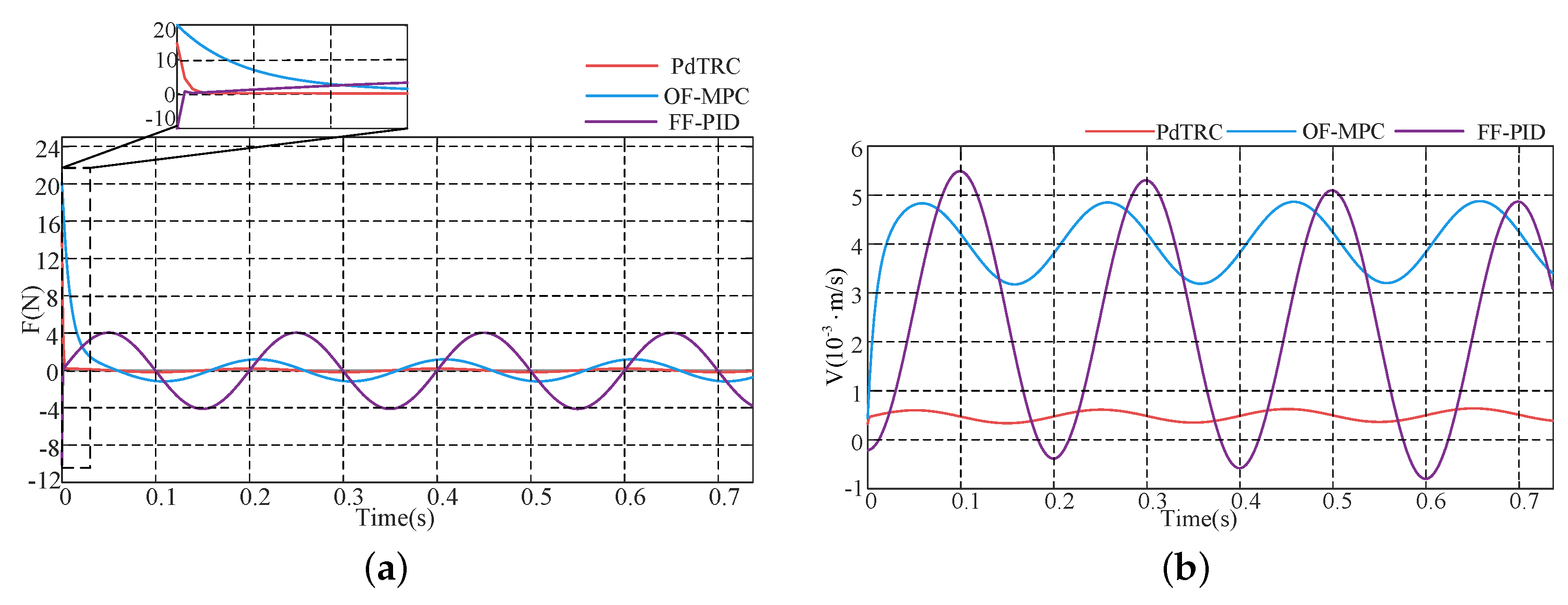
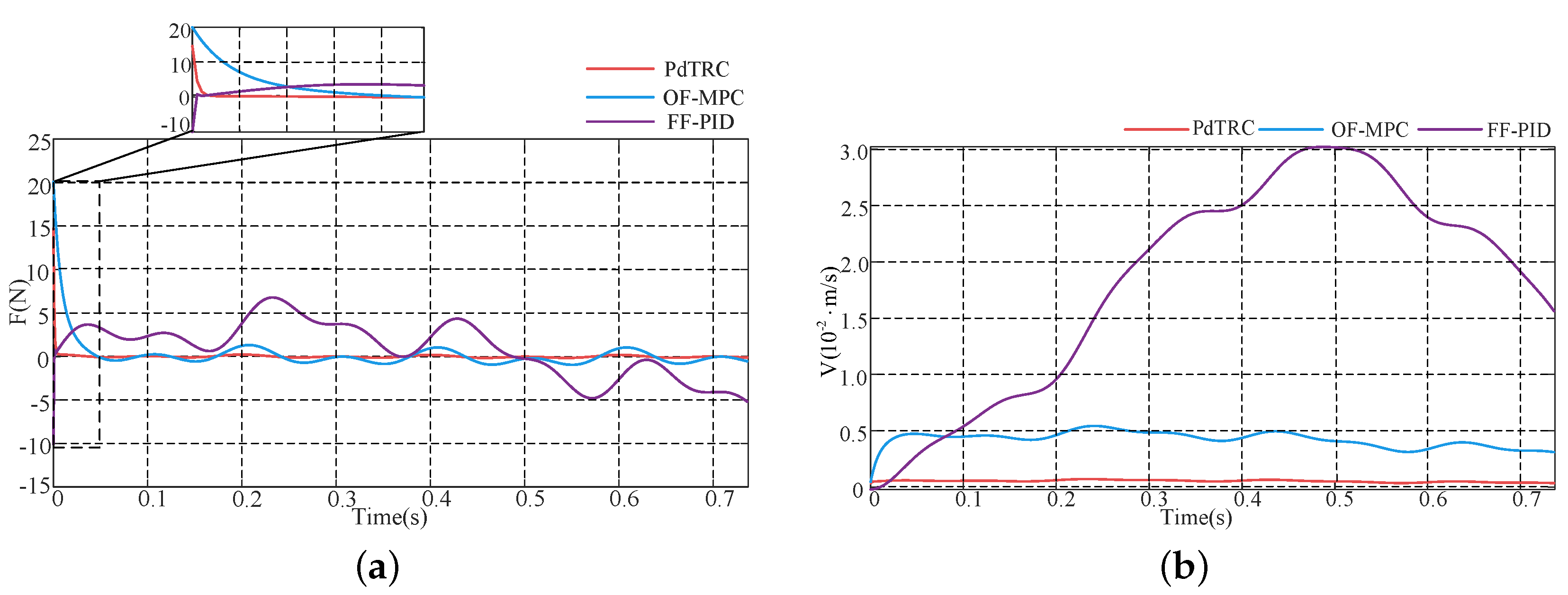
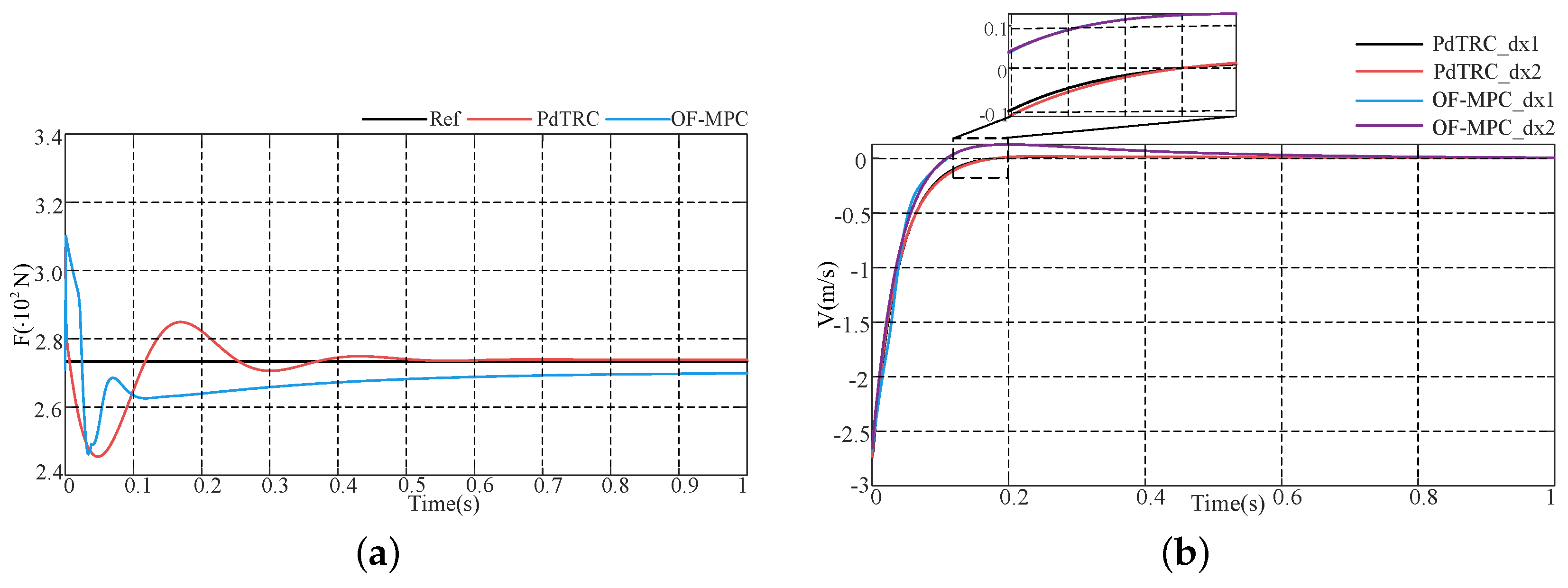
4.1. The Numerical Simulation for Descent Phase

In this scenario, the parameters of the predefined-time (PdT) controller and observer are set to $T_o=0.02\mathrm{s}$ and $T_p=0.05\mathrm{s}$, respectively. Other control parameters are chosen as $\delta =0.5$, $\alpha =0.9$, $\beta =0.9$, $k=20$, and $\eta =0.1$. The initial drop height is $h=1\mathrm{m}$ and the initial angular velocity is $\omega =0$. Specifically, to simulate scenarios on other planets, the desired acceleration is $a_r={\displaystyle \frac{1}{6}}\mathrm{g}$ for the Moon and $a_r=0.38\mathrm{g}$ for Mars. The corresponding desired angular acceleration and desired angular velocity are $\dot{\omega }={\displaystyle \frac{a_r}{R}}$ and ${\omega }_r={\displaystyle \frac{a_{r}t}{R}}$, respectively. $R=0.08\mathrm{m}$ denotes the radius of the drum.

Sinusoidal disturbances are commonly observed in cable-driven robotic systems due to cable resonance and periodic tension variations [47]. Therefore, to emulate such realistic scenarios, two types of disturbances are applied in the simulation: (i) a single-frequency sinusoidal disturbance $d_1$, and (ii) a composite sinusoidal disturbance $d_2$ composed of multiple frequency components. Their specific expressions are given by following:

$$\begin{array}{cc}\hfill d_1& =sin\left(10\pi t\right),\hfill \\ \hfill d_2& =sin\left(2\pi t\right)+0.5sin\left(10\pi t\right)+0.3sin\left(20\pi t\right).\hfill \end{array}$$

While sinusoidal disturbances are representative of structural oscillations in cable-driven systems, we acknowledge that non-periodic or random disturbances may also occur in practice. Evaluating the observer performance under such unstructured disturbances will be considered in future research.

The trajectories of the PdTDO under two types of disturbances are recorded in Figure 3. Figure 3 indicates that the proposed PdTDO provides an efficient compensation for the controller design. The estimation error of the external disturbances converges to the neighborhood of the origin within a PdT $T_o$. Specifically, the estimation errors can be bounded by $0.04$.

The comparative simulations of the force and velocity tracking errors during the descent phase under sinusoidal disturbances $d_1$ and $d_2$ are shown in Figure 4 (lunar simulation) and Figure 5 (Mars simulation).

Figure 4 and Figure 5 present the comparative response curves of the system under three different control frameworks. As observed from Figure 4a and Figure 5a, all three controllers are capable of maintaining the force tracking error within $20\mathrm{N}$. However, although the FF-PID controller guarantees system stability, it consistently exhibits considerable phase lag, resulting in a sinusoidal tracking error with an amplitude of approximately $4\mathrm{N}$. In comparison, the OF-MPC approach demonstrates slightly improved performance, yet its relatively large initial control error may cause potential damage to physical hardware, which limits its practical applicability. In contrast, the proposed PdT control method maintains significantly smaller steady-state and initial tracking errors. These results validate the effectiveness, robustness, and superiority of the proposed control strategy.

Thereafter, we further demonstrate our proposed method under disturbance $d_2$, and the corresponding results are given in Figure 6 and Figure 7.

Figure 6 and Figure 7 illustrate the comparative response curves of the system under three different control frameworks. As shown in Figure 6a and Figure 7a, the proposed PdTRC method exhibits an initial force tracking error of approximately $10\mathrm{N}$. With the introduction of the PdTDO, the tracking error is further reduced to within $1\mathrm{N}$, and the velocity error is also suppressed to below $3.0\times {10}^{-3}\mathrm{m}/\mathrm{s}$ within the predefined time $T_p$. In contrast, the FF-PID controller produces oscillatory force tracking errors as high as $\pm 7\mathrm{N}$, with a maximum velocity error reaching $3.0\times {10}^{-2}\mathrm{m}/\mathrm{s}$—nearly ten times that of the PdTRC. While the output-feedback model predictive control (OF-MPC) method achieves slightly better performance than FF-PID, it still performs worse than the proposed PdT-based approach. Moreover, the substantial computational burden of OF-MPC makes it unsuitable for real-time applications such as low-gravity simulation systems, where high responsiveness is essential. In summary, the proposed PdT control method not only achieves fast convergence but also ensures small tracking errors, thereby further validating its superior performance.

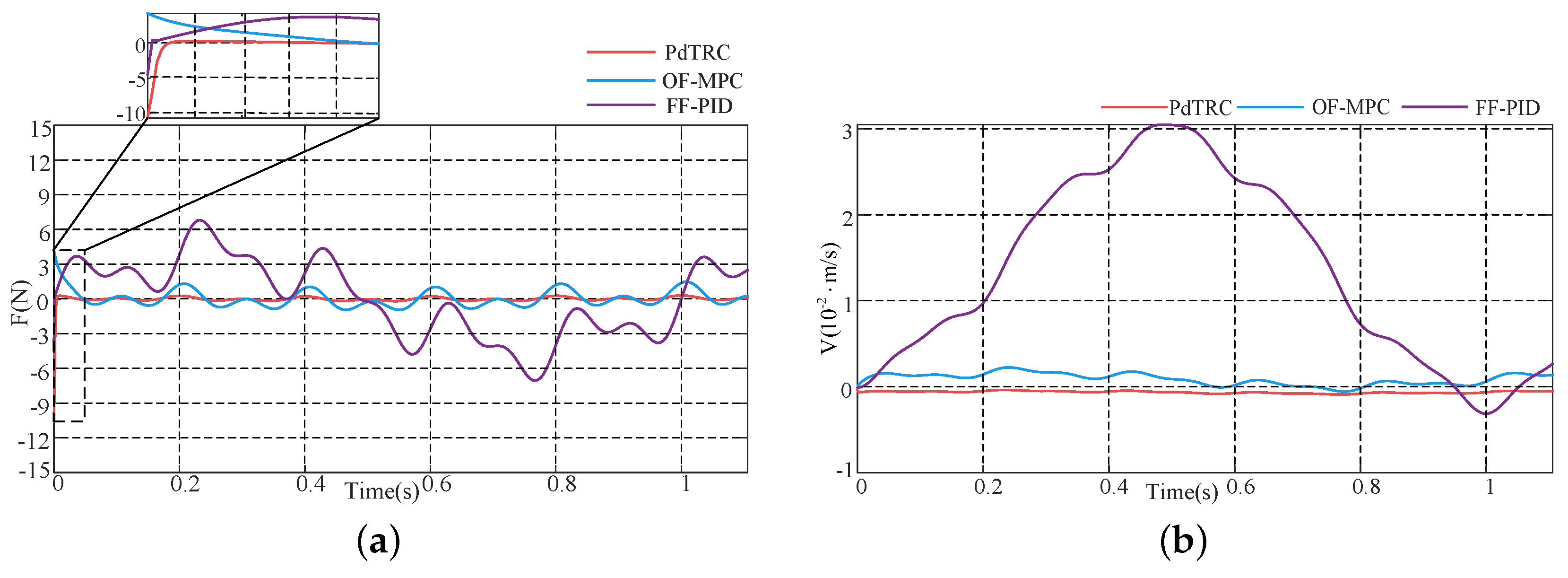
4.2. The Numerical Simulation for Landing Buffering Phase

This subsection illustrates some simulation demonstrations of the landing buffering phase. The parameters of the controller (29) are $\lambda =0.4$ and $k=10$. The vertical position at the moment of touchdown is $h=0$, and a buffering stroke of $l=0.08\mathrm{m}$ is considered for the load.

The simulation results are recorded in Figure 8 and Figure 9, in which the control performance of the PdT controller and OF-MPC is compared under simulated lunar and Mars low-gravity landing scenarios. The results demonstrate that both controllers are capable of maintaining the maximum force tracking error within $30\mathrm{N}$, meeting the requirements for landing buffering. However, compared with OF-MPC, PdTRC enables the system force to converge to the reference value $F_r$ faster. Moreover, the velocity ${\dot{x}}_1$ and ${\dot{x}}_2$ under PdTRC also converge faster than those under OF-MPC, facilitating a smoother dynamic transition during the landing phase. In summary, the PdT controller proposed in this study demonstrates superior overall performance in terms of both control accuracy and convergence speed, offering enhanced robustness and engineering applicability in low-gravity simulation environments.

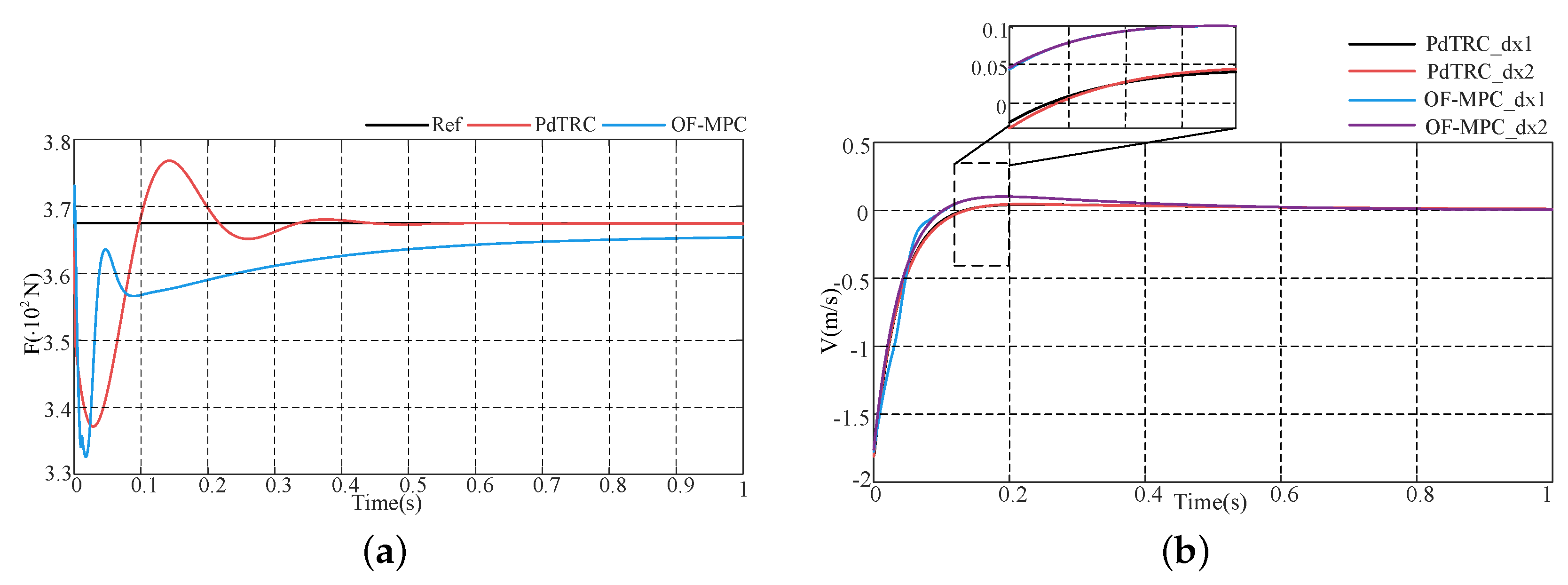
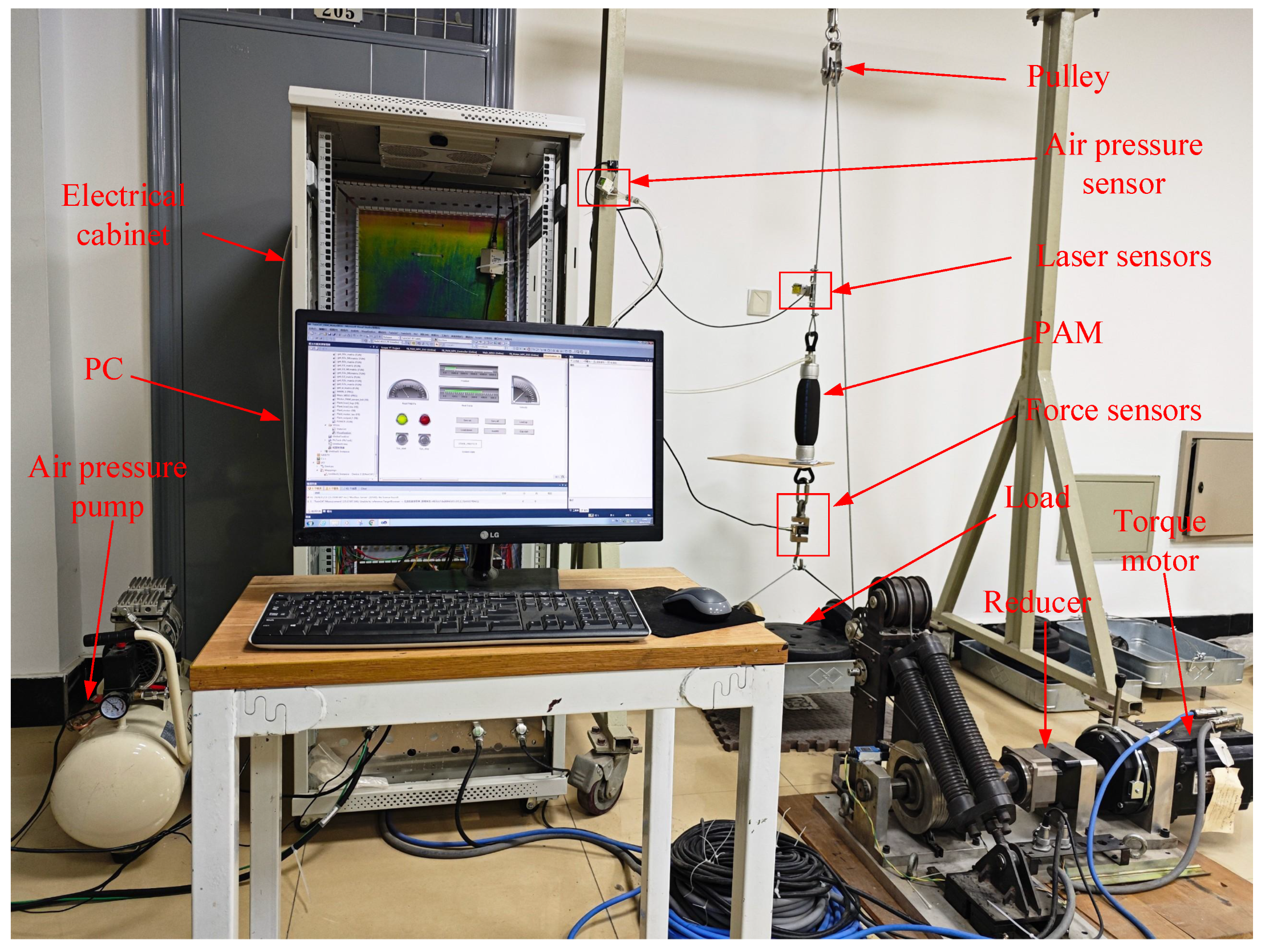
5. Physical Experiments

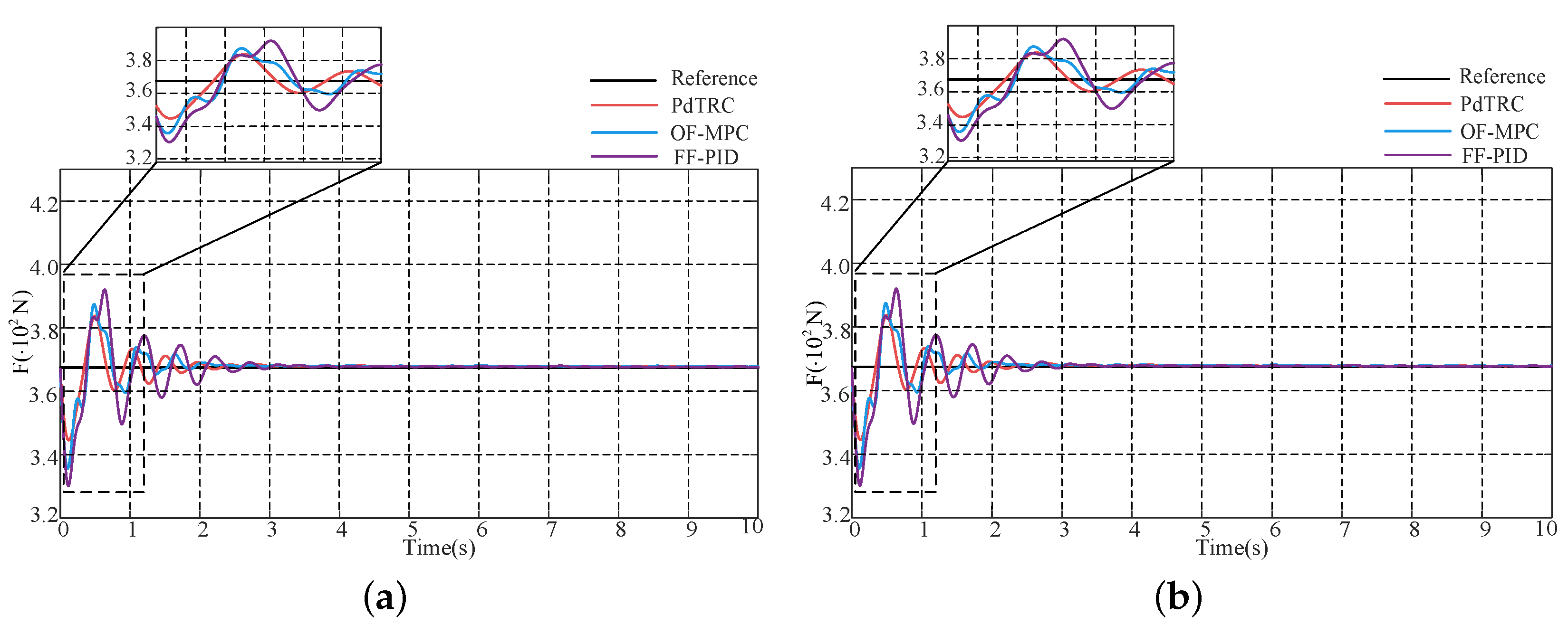
The SCF experimental platform, shown in Figure 10, consists of a torque motor, a PAM, and various sensors. The torque motor is responsible for lifting the suspended load and controlling its descent to simulate micro- and low-gravity conditions. Meanwhile, the PAM is utilized as an active landing buffer to mitigate impact forces during touchdown. The platform integrates multiple sensors to monitor the internal pressure of the PAM, the compression displacement, and the vertical output force of the load in real-time. The sensor measurements are transmitted in real time to the PC control unit. Moreover, the modular structure of the platform allows for rapid switching between control modes and experimental configurations, thereby supporting flexible validation of both descent and landing-buffering phases.

A. 

The landing buffering scenario under low-gravity conditions

In the experiment, a tray platform is used to emulate the dynamic characteristics of a landing spacecraft. For the landing impact tests conducted under simulated lunar and Mars low-gravity conditions, the mass of the tray platform is $m=45\mathrm{kg}$. Based on the gravitational acceleration values for the Moon and Mars, the SGO system is required to deliver a constant vertical support force of $367.5\mathrm{N}$ and a directional unloading force of $273.42\mathrm{N}$ to accurately simulate the low-gravity environments. The control performance of the proposed robust predefined-time controller is compared with those of an OF-MPC controller and an FF-PID controller. To assess the effectiveness and robustness of the proposed control approach, a comparative study is carried out against two baseline controllers: an OF-MPC and an FF-PID. The evaluation focuses on landing impact mitigation, force tracking accuracy, and convergence performance under external disturbances and unmodeled dynamics. This comparison highlights the practical advantages of the proposed robust predefined-time controller in real-time SGO applications.

Figure 11 illustrates that, in landing-buffer experiments under simulated lunar and Martian low-gravity conditions, the proposed PdTRC method confines the force error within $25\mathrm{N}$ and achieves a rapid settling time. However, both the OF-MPC and FF-PID controllers produced maximum force errors exceeding $30\mathrm{N}$; notably, the FF-PID peaking near $40\mathrm{N}$ and showed an excessively long settling time. Furthermore, the PdTRC consistently limits its maximum force error to the $25\mathrm{N}$ specification, fully satisfying the design requirements. This robust accuracy under varying impact disturbances underscores the method’s suitability for real-time control in low-gravity landing systems.

B. 

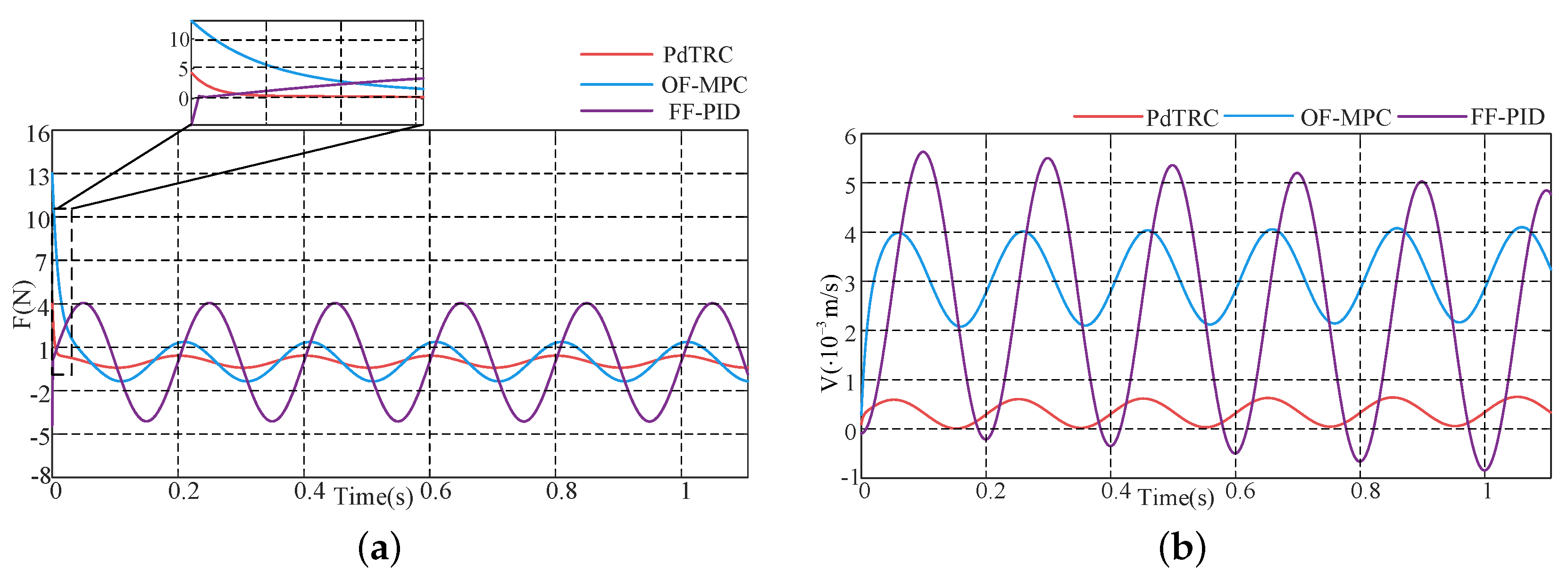
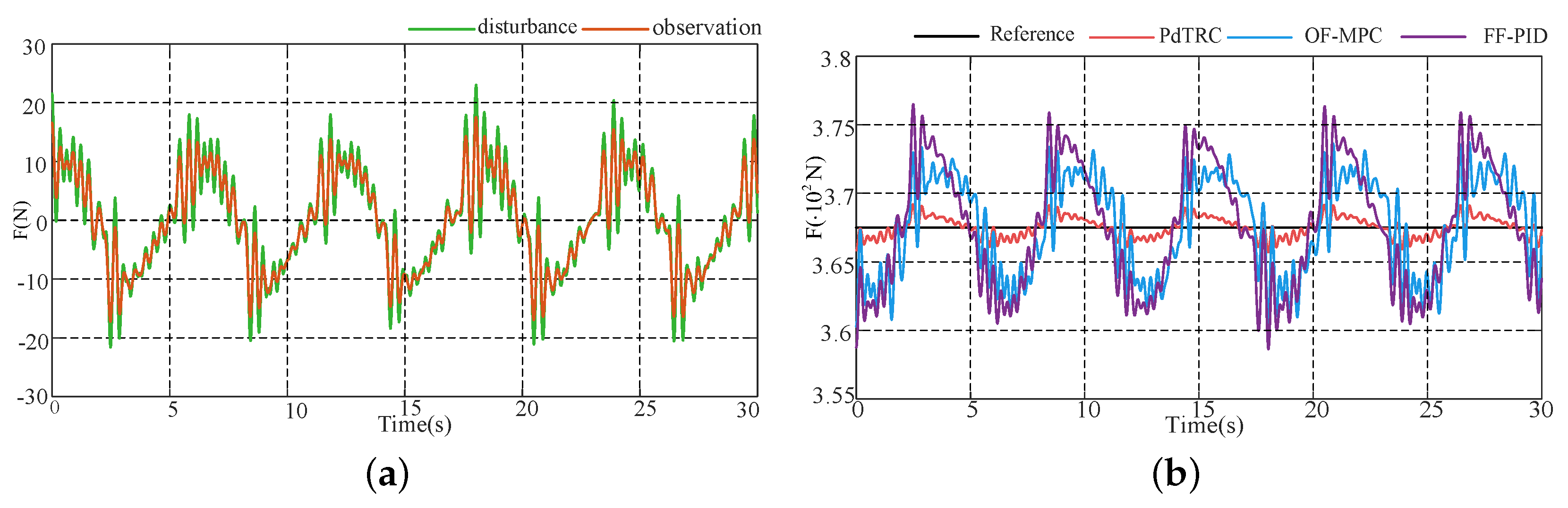
Disturbance rejection scenario

Due to the complex surface conditions on the Moon and Mars, the movement of lunar rovers, Mars rovers, and astronauts may introduce disturbances to the system. However, the SGO system must continuously provide a constant upward offloading force to achieve a stable low-gravity environment simulation. Therefore, the SGO system must possess strong disturbance rejection capabilities. In the experiments, irregular disturbances with a peak amplitude of 20 N were injected into the SCF system to emulate real-world perturbations, and the disturbance-rejection performance of the proposed robust predefined-time controller was compared against that of an OF-MPC and an FF-PID controller.

Figure 12a illustrates that the proposed PdTDO accurately estimates irregular disturbances and guarantees that the estimation error converges within $2\mathrm{N}$ within the predefined time. As shown in Figure 12b, PdTRC developed based on the PdTDO, effectively suppresses irregular disturbances under simulated low-gravity conditions, maintaining the disturbance within $3\mathrm{N}$. In comparison, the maximum disturbance errors of the FF-PID and OF-MPC controllers reach approximately $10\mathrm{N}$, indicating inferior disturbance rejection performance compared to the proposed PdTRC. These results further validate the robustness and superiority of the PdTRC in scenarios involving uncertain external disturbances.

6. Conclusions

This paper presents a novel control framework for suspended gravity offloading (SGO) systems, integrating a predefined-time disturbance observer with a predefined-time robust controller to overcome the challenge of guaranteeing deterministic convergence under uncertain dynamics and external disturbances. First, a predefined-time disturbance observer is employed to estimate the system’s unmodeled dynamics and uncertain external disturbances. Next, a predefined-time robust controller is designed based on the observer’s estimates. Furthermore, a pneumatic artificial muscle is integrated to physically mitigate the underactuation inherent in conventional SGO systems, and a predefined-time active buffering control strategy is developed based on the PAM. Finally, the efficacy and robustness of the proposed framework are validated through extensive numerical simulations and physical experiments.

References

1. Wang, Y.; Gao, J.; Ma, Z.; Li, Y.; Zuo, S.; Liu, J. Design and verification of an active lower limb exoskeleton for micro-low gravity simulation training. In Proceedings of the International Conference on Intelligent Robotics and Applications, Harbin, China, 1–3 August 2022; Springer: Berlin/Heidelberg, Germany, 2022; pp. 114–123. [Google Scholar]
2. Hou, W.; Hao, Y.; Wang, C.; Chen, L.; Li, G.; Zhao, B.; Wang, H.; Wei, Q.; Xu, S.; Feng, K.; et al. Theoretical and experimental investigations on high-precision micro-low-gravity simulation technology for lunar mobile vehicle. Sensors 2023, 23, 3458. [Google Scholar] [CrossRef] [PubMed]
3. Li, C.; Wang, H.; Hu, Z.; Wang, C.; Chen, J. Design and analysis of low-gravity simulation scheme for mars ascent vehicle. Aerospace 2024, 11, 424. [Google Scholar] [CrossRef]
4. Jarvis, S.L.; Vu, L.Q.; Gupta, G.; Benson, E.; Kim, K.H.; Rhodes, R.; Rajulu, S.L. Development of ARGOS (Active Response Gravity Offload System) Offloading Assessments and Methodology for Lunar EVA Simulations. In Proceedings of the 52nd International Conference on Environmental Systems, Calgary, Canada, 12–16 July 2023. [Google Scholar]
5. Xiong, D.; Huang, Y.; Yang, Y.; Liu, H.; Jiang, Z.; Han, W. Research on Horizontal Following Control of a Suspended Robot for Self-Momentum Targets. In Proceedings of the 2023 IEEE International Conference on Robotics and Biomimetics (ROBIO), Koh Samui, Thailand, 4–9 December 2023; pp. 1–6. [Google Scholar]
6. Kim, Y.D.; Kim, S.Y.; Park, K.H. Development of the six degree-of-freedom active vibration isolation system by using a phase compensated velocity sensor. Trans. Korean Soc. Mech. Eng. A 2009, 33, 1347–1352. [Google Scholar] [CrossRef]
7. Könemann, T.; Kaczmarczik, U.; Gierse, A.; Greif, A.; Lutz, T.; Mawn, S.; Siemer, J.; Eigenbrod, C.; von Kampen, P.; Lämmerzahl, C. Concept for a next-generation drop tower system. Adv. Space Res. 2015, 55, 1728–1733. [Google Scholar] [CrossRef]
8. Sanavandi, H.; Guo, W. A magnetic levitation based low-gravity simulator with an unprecedented large functional volume. NPJ Microgravity 2021, 7, 40. [Google Scholar] [CrossRef]
9. Wang, A.; Wang, S.; Xia, H.; Ma, G. Dynamic modeling and control for a double-state microgravity vibration isolation system. Microgravity Sci. Technol. 2023, 35, 9. [Google Scholar] [CrossRef]
10. Tanimoto, R.; Moore, A.; MacDonald, D.; Thomas, S.; Murray, A.; Polanco, O.; Agnes, G. Model and test validation of gravity offload system. In Proceedings of the 48th AIAA/ASME/ASCE/AHS/ASC Structures, Structural Dynamics, and Materials Conference, Honolulu, HI, USA, 23–26 April 2007; p. 1790. [Google Scholar]
11. Orr, S.; Casler, J.; Rhoades, J.; de León, P. Effects of walking, running, and skipping under simulated reduced gravity using the NASA Active Response Gravity Offload System (ARGOS). Acta Astronaut. 2022, 197, 115–125. [Google Scholar] [CrossRef]
12. Wei, J.; Cao, D.; Wang, L.; Huang, H.; Huang, W. Dynamic modeling and simulation for flexible spacecraft with flexible jointed solar panels. Int. J. Mech. Sci. 2017, 130, 558–570. [Google Scholar] [CrossRef]
13. Liu, Y. Robust adaptive observer for nonlinear systems with unmodeled dynamics. Automatica 2009, 45, 1891–1895. [Google Scholar] [CrossRef]
14. Liu, P.; Yu, H.; Cang, S. Adaptive neural network tracking control for underactuated systems with matched and mismatched disturbances. Nonlinear Dyn. 2019, 98, 1447–1464. [Google Scholar] [CrossRef]
15. Bianchi, D.; Di Gennaro, S.; Di Ferdinando, M.; Acosta Lùa, C. Robust control of uav with disturbances and uncertainty estimation. Machines 2023, 11, 352. [Google Scholar] [CrossRef]
16. Zhou, F.; Peng, H.; Zeng, X.; Tian, X.; Peng, X. RBF-ARX model-based robust MPC for nonlinear systems with unknown and bounded disturbance. J. Frankl. Inst. 2017, 354, 8072–8093. [Google Scholar] [CrossRef]
17. Wang, N.; Sun, Z.; Su, S.F.; Wang, Y. Fuzzy uncertainty observer-based path-following control of underactuated marine vehicles with unmodeled dynamics and disturbances. Int. J. Fuzzy Syst. 2018, 20, 2593–2604. [Google Scholar] [CrossRef]
18. Moulay, E.; Léchappé, V.; Bernuau, E.; Defoort, M.; Plestan, F. Fixed-time sliding mode control with mismatched disturbances. Automatica 2022, 136, 110009. [Google Scholar] [CrossRef]
19. Hu, Y.; Yan, H.; Zhang, H.; Wang, M.; Zeng, L. Robust adaptive fixed-time sliding-mode control for uncertain robotic systems with input saturation. IEEE Trans. Cybern. 2022, 53, 2636–2646. [Google Scholar] [CrossRef]
20. Liu, H.; Zhang, T. Neural network-based robust finite-time control for robotic manipulators considering actuator dynamics. Robot. Comput. Integr. Manuf. 2013, 29, 301–308. [Google Scholar] [CrossRef]
21. Tajrishi, M.A.Z.; Kalat, A.A. Fast finite time fractional-order robust-adaptive sliding mode control of nonlinear systems with unknown dynamics. J. Comput. Appl. Math. 2024, 438, 115554. [Google Scholar] [CrossRef]
22. Wang, H.; Xu, K.; Zhang, H. Adaptive finite-time tracking control of nonlinear systems with dynamics uncertainties. IEEE Trans. Autom. Control. 2022, 68, 5737–5744. [Google Scholar] [CrossRef]
23. Wang, F.; You, Z.; Liu, Z.; Chen, C.P. A fast finite-time neural network control of stochastic nonlinear systems. IEEE Trans. Neural Netw. Learn. Syst. 2022, 34, 7443–7452. [Google Scholar] [CrossRef]
24. Dorato, P. An overview of finite-time stability. In Current Trends in Nonlinear Systems and Control: In honor of Petar Kokotović and Turi Nicosia; Springer: Berlin/Heidelberg, Germany, 2006; pp. 185–194. [Google Scholar]
25. Amato, F.; Ambrosino, R.; Ariola, M.; Cosentino, C.; De Tommasi, G. Finite-Time Stability and Control; Springer: London, UK, 2014; Volume 453. [Google Scholar]
26. Yan, H.; Lu, H.; Wang, H.; Zhang, Z.; Huang, X. Neural-Network-Based Nonlinear Model Predictive Control of Suspension Gravity Offload System. In Proceedings of the 2024 3rd Conference on Fully Actuated System Theory and Applications (FASTA), Shenzhen, China, 10–12 May 2024; pp. 1346–1351. [Google Scholar] [CrossRef]
27. Duan, H.; Yuan, Y.; Zeng, Z. Automatic carrier landing system with fixed time control. IEEE Trans. Aerosp. Electron. Syst. 2022, 58, 3586–3600. [Google Scholar] [CrossRef]
28. Liu, K.; Wang, Y.; Li, Y.; Zhang, Y.; Wen, C.Y. Velocity-Free Adaptive Neural-Fuzzy Predefined-Time Attitude Control for Spacecraft. IEEE Trans. Aerosp. Electron. Syst. 2025, 1–17. [Google Scholar] [CrossRef]
29. Li, Y.; Wang, T.; Liu, X.; Wen, C.y. Predefined-time Active Fault-tolerant Control of Transport Aircraft Subject to Control Surface Failures. IEEE Trans. Aerosp. Electron. Syst. 2024, 1–14. [Google Scholar] [CrossRef]
30. Munoz-Vazquez, A.J.; Sánchez-Torres, J.D.; Jimenez-Rodriguez, E.; Loukianov, A.G. Predefined-time robust stabilization of robotic manipulators. IEEE/ASME Trans. Mechatronics 2019, 24, 1033–1040. [Google Scholar] [CrossRef]
31. Ai, Z.; Wang, H. Adaptive predefined-time tracking control of nonlinear systems with unmodeled dynamics. Int. J. Control. 2025, 1–10. [Google Scholar] [CrossRef]
32. Wang, Q.; Cao, J.; Liu, H. Adaptive fuzzy control of nonlinear systems with predefined time and accuracy. IEEE Trans. Fuzzy Syst. 2022, 30, 5152–5165. [Google Scholar] [CrossRef]
33. Muñoz-Vázquez, A.J.; Fernández-Anaya, G.; Sánchez-Torres, J.D.; Meléndez-Vázquez, F. Predefined-time control of distributed-order systems. Nonlinear Dyn. 2021, 103, 2689–2700. [Google Scholar] [CrossRef]
34. Sun, G.; Liu, Q.; Pan, F.; Zheng, J. Disturbance observer based adaptive predefined-time sliding mode control for robot manipulators with uncertainties and disturbances. Int. J. Robust Nonlinear Control. 2024, 34, 12349–12374. [Google Scholar] [CrossRef]
35. Liu, Y.; Huo, Y. Predefined-time sliding mode control of chaotic systems based on disturbance observer. Math. Biosci. Eng. 2024, 21, 5032–5046. [Google Scholar] [CrossRef]
36. Ji, J.; Jiang, P. Research on Predefined Time Sliding Mode Control Method for High-Speed Maglev Train Based on Finite Time Disturbance Observer. Actuators 2025, 14, 21. [Google Scholar] [CrossRef]
37. Zhao, Z.L.; Guo, B.Z. A novel extended state observer for output tracking of MIMO systems with mismatched uncertainty. IEEE Trans. Autom. Control. 2017, 63, 211–218. [Google Scholar] [CrossRef]
38. Besnard, L.; Shtessel, Y.B.; Landrum, B. Control of a quadrotor vehicle using sliding mode disturbance observer. In Proceedings of the 2007 American Control Conference, New York, NY, USA, 9–13 July 2007; pp. 5230–5235. [Google Scholar]
39. Kögel, M.; Findeisen, R. Robust output feedback MPC for uncertain linear systems with reduced conservatism. IFAC-PapersOnLine 2017, 50, 10685–10690. [Google Scholar] [CrossRef]
40. Zhang, D.; Zhao, X.; Han, J. Active model-based control for pneumatic artificial muscle. IEEE Trans. Ind. Electron. 2016, 64, 1686–1695. [Google Scholar] [CrossRef]
41. Sánchez-Torres, J.D.; Gómez-Gutiérrez, D.; López, E.; Loukianov, A.G. A class of predefined-time stable dynamical systems. IMA J. Math. Control. Inf. 2018, 35, i1–i29. [Google Scholar] [CrossRef]
42. Wang, Y.; Gao, J.; Wu, X.; Feng, X. Predefined-time tracking control for a class of strict-feedback nonlinear systems with time-varying actuator failures and input delay. Nonlinear Dyn. 2025, 113, 11577–11591. [Google Scholar] [CrossRef]
43. Ni, J.; Shi, P. Global predefined time and accuracy adaptive neural network control for uncertain strict-feedback systems with output constraint and dead zone. IEEE Trans. Syst. Man Cybern. Syst. 2020, 51, 7903–7918. [Google Scholar] [CrossRef]
44. Wu, C.; Yan, J.; Shen, J.; Wu, X.; Xiao, B. Predefined-time attitude stabilization of receiver aircraft in aerial refueling. IEEE Trans. Circuits Syst. II Express Briefs 2021, 68, 3321–3325. [Google Scholar] [CrossRef]
45. Jiménez-Rodríguez, E.; Muñoz-Vázquez, A.J.; Sánchez-Torres, J.D.; Defoort, M.; Loukianov, A.G. A Lyapunov-like characterization of predefined-time stability. IEEE Trans. Autom. Control. 2020, 65, 4922–4927. [Google Scholar] [CrossRef]
46. Bingul, Z.; Gul, K. Intelligent-PID with PD feedforward trajectory tracking control of an autonomous underwater vehicle. Machines 2023, 11, 300. [Google Scholar] [CrossRef]
47. Zarebidoki, M.; Dhupia, J.S.; Xu, W. A review of cable-driven parallel robots: Typical configurations, analysis techniques, and control methods. IEEE Robot. Autom. Mag. 2022, 29, 89–106. [Google Scholar] [CrossRef]
Figure 1. Structure of a suspension-based gravity offloading (SGO) system. The red square indicates the SCF (suspension constant force) subsystem, which is responsible for active offloading. PAM: pneumatic artificial muscle.
Aerospace 12 00495 g001
Figure 2. Structure of a suspension constant force (SCF) subsystem. The variables x 1 , x 2 , and x 3 represent the displacements of the pulley, load, and landing spring compression, respectively. Positive directions are indicated by upward arrows in the figure. The reference zero positions are defined as follows: x 1 = 0 and x 2 = 0 both correspond to the state where the load just contacts the ground without inducing spring compression, while x 3 = 0 represents the uncompressed spring.
Aerospace 12 00495 g002
Figure 3. Comparison between the disturbance and its estimation by the PdTO: (a) single-frequency sinusoidal disturbance d 1 ; (b) composite sinusoidal disturbance d 2 .
Aerospace 12 00495 g003
Figure 4. Force and velocity tracking errors during the descent phase under simulated lunar gravity with a single-frequency sinusoidal disturbance: (a) force error comparison; (b) velocity error comparison.
Aerospace 12 00495 g004
Figure 5. Force and velocity tracking errors during the descent phase under simulated Martian gravity with a single-frequency sinusoidal disturbance: (a) force error comparison; (b) velocity error comparison.
Aerospace 12 00495 g005
Figure 6. Force and velocity tracking errors during the descent phase under simulated lunar gravity with a composite sinusoidal disturbance: (a) force error comparison; (b) velocity error comparison.
Aerospace 12 00495 g006
Figure 7. Force and velocity tracking errors during the descent phase under simulated Martian gravity with a composite sinusoidal disturbance: (a) force error comparison; (b) velocity error comparison.
Aerospace 12 00495 g007
Figure 8. Force and velocity tracking during lunar landing: (a) force comparison under PdTRC and OF-MPC; (b) velocity comparison between control methods.
Aerospace 12 00495 g008
Figure 9. Force and velocity tracking during Martian landing: (a) force comparison under PdTRC and OF-MPC; (b) velocity comparison between control methods.
Aerospace 12 00495 g009
Figure 10. The SCF experimental platform setup.
Aerospace 12 00495 g010
Figure 11. Landing-buffer force tracking comparison under simulated low-gravity conditions: (a) lunar, (b) Martian.
Aerospace 12 00495 g011
Figure 12. Disturbance estimation and rejection under simulated lunar constant-force control: (a) actual disturbance vs. observer estimate; (b) disturbance suppression performance.
Aerospace 12 00495 g012
Disclaimer/Publisher’s Note: The statements, opinions and data contained in all publications are solely those of the individual author(s) and contributor(s) and not of MDPI and/or the editor(s). MDPI and/or the editor(s) disclaim responsibility for any injury to people or property resulting from any ideas, methods, instructions or products referred to in the content.