Development of a Simulation Model for Blade Tip Timing with Uncertainties

Abstract

Blades are widely used in the engines of aerospace vehicles, fans of near-space aerostat, and other equipment, and they are the key to completing energy conversion and pressure adjustment of the capsule. Blade tip timing (BTT) is the most cost-efficient approach for the monitoring of blades. The reliability and validity of BTT is mainly investigated through numerical simulation and experimental verification. However, not all researchers are able to carry out the expensive and time-consuming task of rotating the blade test bench and its monitoring systems. Therefore, a good and easily understood simulator is necessary. In this paper, an effective BTT simulation model that is capable of considering various uncertainties such as installation errors, probe accuracy, sampling clock frequency, speed fluctuations, and mistuning is presented. A blade multi-harmonic vibration model is also presented, which is not only easy to implement but also simplifies the solution of dynamic equations. Also, the simulation results show that the proposed model is accurate and consistent with the experimental results. This will help researchers to achieve an improved understanding of BTT and form the basis for conducting research in related areas in a short period of time.

1. Introduction

Blades are the core component for aerospace equipment and their operational safety is extremely important. Due to multiple excitation sources, the forced vibration response of the blades of a turbine (e.g., aero-engine) may occur at or near the natural frequency. The structural movement of the blade assembly affects fatigue life, and blade safety has historically been emphasized by designers and users. Currently, blade tip timing (BTT) is regarded as the most convenient and effective blade-monitoring technique. It functions by utilizing the time of arrival (ToA) of the blade tip to estimate the vibration displacement of the blade tip as it crosses the probe.

To carry out simulation and comparison of BTT methods, the development of appropriate simulators is necessary. Carrington et al. [1,2] proposed a simulator that is capable of obtaining blade vibration displacements, as well as the displacements measured by the blade tip timing probe at specific mounting angles. The simulator, which comprises four blades, each idealized as a single mass-spring-damper system, is implemented with MATLAB (https://www.mathworks.com/products/matlab.html, accessed on 10 May 2025) and SIMULINK (https://www.mathworks.com/products/simulink.html, accessed on 10 May 2025) for model solving and probe-triggering simulations. This model has served as a foundation for numerous subsequent studies. For instance, S. Bornassi et al. [3] built upon this model and put forward a 2-degree-of-freedom (2DoF) blade model. Their objective was to explore the impact of bladed disk resonance on the post-processing method for the blade tip timing (BTT) method, as documented in the reference. Each sector of the bladed disk is simplified as two masses (one represents the blade mass and the other one represents the disk sector mass). Although the model can address certain novel issues, it is constrained by an over-simplification of the tip timing method’s sampling process. Specifically, it continues to overlook the transformation process from the ToA to the vibration displacement. This type of model can only be used for the analysis and validation of post-processing methods for the BTT method.

To explore the influence of various experimental variables of calculating blade vibration displacements from the ToA data and to verify the optimization methodology, it is necessary to transform the blade displacements obtained in the model to acquire the ToA. Fan et al. [4] generated BTT sensor displacements for BTT method validation directly based on vibration parameters and the vibration response signal. Li et al. [5] proposed a simultaneous measurement method of BTC and BTT with a single microwave sensor termed amplitude and phase joint analysis (APJA) method to calibrate critical baseband signals. D. Heller [6] et al. constructed a model for capacitive sensors used in BTT and BTC based on experimental waveform data and developed a new method for analyzing multi-harmonic vibrations. To validate the sparse reconstruction method for under-sampled BTT signals, Huang et al. [7] used the theoretical equations to obtain the vibration displacements and vibration velocities of the blades directly instead of solving the bladed disk dynamics model. These models do not rely on time-dependent equations of motion. They can easily simulate blade vibration displacement and the sensor sampling process at a fixed rotational speed. However, they ignore the impact of rotational speed fluctuations on the BTT method and blade vibration. As a result, they are not suitable for simulating and validating more complex working conditions.

Nikpour et al. [8] proposed a bladed assembly considering the centrifugal effect of the rotational speed for BTT numerical simulations. Mohamed et al. [9] presented a realistic simulator based on the experimentally validated finite element model of a blisk. The method can achieve simulation by solving modal equations of motion to probe triggering, but it fails to consider the effects of uncertainties of the BTT method. Furthermore, the model is still complex, making it difficult to achieve rapid simulation, especially for high sampling frequency, and for multi-blade and multi-sensor systems. Tocci et al. [10] proposed a state space-based approach for generating synthetic tip-timing signals. But, only the synchronous vibrations of blades with a single vibration mode were simulated.

New methods often need to verify their robustness. In numerous studies, the simulation of signals with specific signal-to-noise ratios has been achieved by adding Gaussian noise to blade vibrations [11,12,13,14]. However, this approach has a significant limitation in that it ignores the impact of factors such as rotational speed and clock sampling rate on the sampling accuracy of tip displacement. The signal-to-noise ratios of the BTT signals obtained from the same sampling system and test rig at different rotational speeds will be different. A more accurate simulator can be built to better understand the uncertainty of the blade tip timing method.

This paper analyzes the principles of BTT and the vibration models of blades. A BTT sampling model considering multiple uncertainties and a blade multi-harmonic vibration model have been constructed. This model achieves simple yet efficient simulations of blade vibrations and BTT sampling processes. The validity and accuracy of this model have been proven by comparing the results with experimental data. It provides a foundation for research aimed at improving BTT methodologies, validating new monitoring algorithms, and advancing related fields.

2. The Principle of BTT

The blade tip timing method generally processes data with one revolution as the basic unit. The once per revolution (OPR) signal serves as the starting and ending marks for each revolution. In any single revolution, the motion process of the rotating blade can be separated into two independent processes: rotational motion along the blade direction and vibration of the blade.

$$\mathsf{\Psi }\left(t\right)={\mathsf{\Phi }}_1\left(t\right)+{\mathsf{\Phi }}_2\left(t\right)$$

(1)

where Ψ(t) represents the total mechanical motion equation of the blade. ${\mathsf{\Phi }}_1\left(t\right)$ is the cumulative rotational arc equation for the blade, used to describe its rotation; ${\mathsf{\Phi }}_2\left(t\right)$ denotes the vibration of the blade in radian at time t, reflecting its response to forces or disturbances. Hence,

$${\mathsf{\Phi }}_2(t)={\displaystyle \frac{q_b\left(t\right)}{R}}$$

(2)

where q_b(t) is the vibration displacement of the b-th blade at time t, which corresponds to the blade’s vibration along the arc length. R is the distance from the blade tip to the axis center, equivalent to the radius of the blade disk. In a general case, R is a function of rotational speed Ω and temperature θ. Thus, it is expressed as R (Ω, θ). The physical processes involved are complex. A function of R with respect to time, R(t), can be generated during simulation based on typical radial elongation trend curves of the rotor and case [15] to enable the uncertainty impact of BTC on the blade tip vibration displacement monitoring and calculation.

The cumulative rotational arc equation ${\mathsf{\Phi }}_1\left(t\right)$ of the blade can be represented as

$${\mathsf{\Phi }}_1(t)=2\pi {\int }_{t_{0\left(n\right)}}^t\mathsf{\Omega }\left(t\right)\mathrm{d}t\left(t\in \left[t_{0\left(n\right)},t_{1\left(n\right)}\right]\right)$$

(3)

where $\mathsf{\Omega }\left(t\right)$ is the rotational speed of the blade, in Hz. $t_{0\left(n\right)}$ is the starting time of the n-th revolution, and $t_{1\left(n\right)}$ is the ending time of the n-th revolution.

In the traditional BTT (T-BTT) method, the rotor speed is calculated based on the time difference between two consecutive OPR signals measured by the OPR sensor. Within one revolution, only one speed value can be obtained, which means it ignores the speed fluctuations. However, in actual operation, rotating machinery often needs to adjust its speed to respond to emergencies or change its operating state, and many faults can also cause sudden changes in speed. Therefore, speed fluctuations within one revolution are unavoidable and cannot be neglected. Usually, simplifying the rotational speed within one revolution as a constant acceleration variation is sufficient to evaluate the performance of BTT in addressing speed fluctuations. Therefore,

$$\mathsf{\Omega }(t)=a_{\left(n\right)}t+f_{0\left(n\right)}$$

(4)

where $a_{\left(n\right)}$ is the acceleration within one revolution. $f_{0\left(n\right)}$ is the rotational speed at the beginning of one revolution.

Substitute Equation (4) into Equation (3) to obtain

$${\mathsf{\Phi }}_1(t)=2\pi \left({\displaystyle \frac{1}{2}}{a}_{\left(n\right)}{\left(t-t_{0\left(n\right)}\right)}^2+f_0\left(t-t_{0\left(n\right)}\right)\right)$$

(5)

The cumulative angle of the blade at sampling time t, which is obtained from Equations (3) and (2), is

$$\mathsf{\Psi }(t)=2\pi \left({\displaystyle \frac{1}{2}}{a}_{\left(n\right)}{\left(t-t_{0\left(n\right)}\right)}^2+f_0\left(t-t_{0\left(n\right)}\right)\right)+{\displaystyle \frac{q_b\left(t\right)}{R\left(t\right)}}$$

(6)

When blade No. b passes through the BTT probe during its n-th revolution, the probe records the ToA, and the accumulated rotational angle within one revolution can be calculated with

$${\mathsf{\Psi }}_b={\mathsf{\Phi }}_{\left(p,b\right)}$$

(7)

where ${\mathsf{\Phi }}_{\left(p,b\right)}$ is the original angular distance between probe No. p and blade No. b, which can be expressed as

$${\mathsf{\Phi }}_{\left(p,b\right)}={\mathsf{\Phi }}_{\left(p,1\right)}+\left(b-1\right){\displaystyle \frac{2\pi }{n_b}}={\mathsf{\Phi }}_{\left(p,1\right)}+{\phi }_b$$

(8)

where ${\mathsf{\Phi }}_{(p,1)}$ is the original angular distance between probe No. p and blade No. 1. $n_{\mathrm{b}}$ is the number of blades on the rotor disk. b is serial number of blade. ${\phi }_b$ is the phase delay of blade No. b.

For the non-OPR BTT method, when the first BTT probe detects the signal as the first blade passes through, sampling is then considered to have officially begun. So,

$${\mathsf{\Phi }}_{\left(\mathrm{1,1}\right)}=0$$

(9)

If the blade is considered to be non-vibrating, then the time it takes for the blade to pass through the BTT probe represents its theoretical ToA, which can be calculated using Equations (6) to (9).

$$\pi a_{\left(n\right)}{\left(t_{\mathrm{t}\left(n,b\right)}-t_{0\left(n\right)}\right)}^2+2\pi f_{0\left(n\right)}\left(t_{\mathrm{t}\left(n,b\right)}-t_{0\left(n\right)}\right)-{\mathsf{\Psi }}_b=0$$

(10)

where $t_{\mathrm{t}\left(n,b\right)}$ is theoretical ToA of blade No. b in n-th revolution. In this paper, the subscript b consistently represents the b-th blade, and the subscript n consistently represents the n-th revolution. Subsequent text will not repeat the explanation of these indices.

3. Blade Vibration Model and BTT Sampling Model

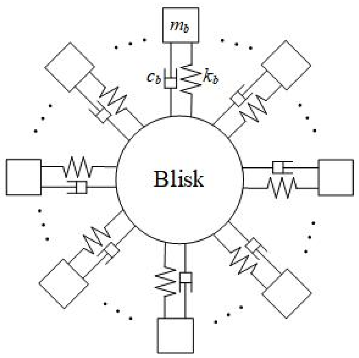
3.1. Blade Vibration Model

In practical applications, rotating blade structures are complex and varied. The complex structure and motion of the blade make it difficult to express mathematically. By employing finite element analysis, the purpose of simplifying the model can be achieved, which facilitates further analysis of BTT and blade vibration. A mathematical model for blade vibration is established based on the FE method. Consequently, the forced vibration differential equation for a multi-degree-of-freedom (MDoF) blade system is

$$\mathbf{M}\ddot{\mathbf{q}}\left(t\right)+\mathbf{C}\dot{\mathbf{q}}\left(t\right)+\mathbf{K}\mathbf{q}\left(t\right)=\mathbf{f}\left(t\right)$$

(11)

where M, C, K are the mass matrix, damping matrix, and stiffness matrix of the blade-disk structure, respectively. f(t) is the excitation force vector, which characterizes the force in each degree of freedom of the blade-disk. q(t) is the vibration displacement vector, which characterizes the vibration displacement of the blades.

In the actual sampling of the BTT, each blade is sampled only once in each revolution as it passes each probe. Therefore, arranging multiple BTT probes at the same axial position actually performs sampling of a single degree of freedom of the blade. To reduce the difficulty of simulation, the blade vibration model in reference [16] is simplified and used, and its mechanical model is shown in Figure 1. The geometric and physical parameters of the rotor elements are assumed to be constant. The Coriolis force, spin softening, and stress stiffening effects are not taken into consideration. If you need to consider these factors, refer to [17], which is helpful for an in-depth analysis of the influence of the actual working conditions and vibration characteristics.

Figure 1. Single-degree-of-freedom (SDoF) blade mechanical model.

The corresponding matrices are

$${\mathbf{M}}_{\left[n_{\mathrm{b}}\times n_{\mathrm{b}}\right]}=\left[\begin{array}{cccc}{m}_1& 0& .& 0\\ 0& m_2& .& 0\\ .& .& .& .\\ 0& 0& .& m_{n_{\mathrm{b}}}\end{array}\right]$$

(12)

$${\mathbf{C}}_{\left[n_{\mathrm{b}}\times n_{\mathrm{b}}\right]}=\left[\begin{array}{cccc}{c}_1& 0& .& 0\\ 0& c_2& .& 0\\ .& .& .& .\\ 0& 0& .& c_{n_{\mathrm{b}}}\end{array}\right]$$

(13)

$${\mathbf{K}}_{\left[n_{\mathrm{b}}\times n_{\mathrm{b}}\right]}=\left[\begin{array}{cccc}{k}_1& 0& .& 0\\ 0& k_2& .& 0\\ .& .& .& .\\ 0& 0& .& k_{n_{\mathrm{b}}}\end{array}\right]$$

(14)

where $m_b\left(b=\mathrm{1,2},\cdots ,n_b\right)$ is the mass of the blade No. b, $c_b$ is the damping of the blade No. b, and $k_b$ is the stiffness of the blade No. b. The subscript $\left[n_{\mathrm{b}}\times n_{\mathrm{b}}\right]$ denotes the size of the matrix.

The blades on the same blade disk are nearly identical, a state known as tuning, which is embodied in the numerical model as

$$\left\{\begin{array}{c}{m}_b=m\\ k_b=k\\ c_b=c\end{array}\right.\left(b=\mathrm{1,2},\cdots ,n_{\mathrm{b}}\right)$$

(15)

The natural frequency ${\omega }^{\mathrm{n}}$ of the blade can be calculated by Equation (16).

$${\omega }^{\mathrm{n}}={\displaystyle \frac{1}{2\pi }}\sqrt{{\displaystyle \frac{k}{m}}}$$

(16)

The damping ratio $\mathsf{\xi }$ of the blade can be calculated by Equation (17).

$$\mathsf{\xi }={\displaystyle \frac{c}{2\sqrt{mk}}}$$

(17)

However, due to a variety of intentional and unintentional reasons, there are small variations in structural or geometric properties between each blade. Mistuning is very common. Numerical simulation of blade mistuning is generally divided into mass mistuning and stiffness mistuning. In this paper, we use mass mistuning to simulate. Correspondingly, the mass of the blade No. b is

$$m_b=m+{\delta }_b(b=\mathrm{1,2},3,\dots ,n_b)$$

(18)

where ${\delta }_b$ is the mistuning mass of the blade No. b, which can be defined as

$${\delta }_b={\delta }_{\mathrm{m}\mathrm{a}\mathrm{x}}\mathrm{r}\mathrm{a}\mathrm{n}\mathrm{d}(\ast )$$

(19)

where ${\delta }_{\mathrm{m}\mathrm{a}\mathrm{x}}$ is the maximum mistuning mass value, $\mathrm{r}\mathrm{a}\mathrm{n}\mathrm{d}\left(\ast \right)$ is a random number function, and the output is a value between −1 and 1.

The excitation force vector $\mathbf{f}\left(t\right)$ can be

$$\mathbf{f}(t)=\left[\begin{array}{c}{f}_1\left(t\right)\\ f_2\left(t\right)\\ ⋮\\ f_{n_b}(t)\end{array}\right]$$

(20)

where $f_b\left(t\right)$ is the force of blade No. b, and can usually be expressed as

$$f_b\left(t\right)=\sum _{i=1}^{F_N}\left[F_{\max \left(b\right)}^i\sin \left(n_i^{\mathrm{E}\mathrm{O}}{\int }_{t_0}^t\mathsf{\Omega }\left(t\right)\mathrm{d}t+{\phi }_{b,i}\right)\right]$$

(21)

where $F_N$ is the number of excitation forces. The subscript i denotes the i-th excitation force. $F_{\max \left(b\right) }$ is the amplitude of the excitation force. $n_i^{\mathrm{E}\mathrm{O}}$ is the engine order (EO) of excitation, and $\mathsf{\Omega }\left(t\right)$ is the blade speed. The phase delay of blade No. b is

$${\phi }_{b,i}={\phi }_{0,i}+{\phi }_b$$

(22)

where ${\phi }_0$ is the initial phase.

A multi-source excitation force model more in line with the actual airflow excitation is proposed in the reference [18,19], and the model is shown in Figure 2.

Figure 2. Multi-source airflow excitation force model.

For a single excitation force, the numerical expression is

$$f_{b,i}\left(t\right)=\left\{\begin{array}{cc}{A}_i& {\phi }_i+2k\pi \le {{\displaystyle \int }}_{t_0}^t\mathsf{\Omega }\left(t\right)\mathrm{d}t-{\phi }_b\le {\phi }_i+2\pi d_i+2k\pi \\ 0& \mathrm{Other} \mathrm{cases}\end{array}\right.$$

(23)

Multiple excitation forces can be represented in the time domain by a square wave function as

$$f_b\left(t\right)=\sum _{i=1}^{N_{\mathrm{F}}}{A}_i\mathrm{squrewave}\left({\mathsf{\Phi }}_1\left(t\right)+{\phi }_i-{\phi }_b,d_i\right)$$

(24)

where $N_{\mathrm{F}}$ is the number of excitation forces. $A_i$ is the amplitude of the i-th force. squarewave (ϕ, duty) is the square wave function which is used to simulate the force shown in Figure 3. The input variable $\varphi$ is time series. $d_i$ is the duty cycle of the square wave function; in this paper, it can be set as $d_i=3\%$. ${\phi }_i$ is the circumferential angle of the excitation force. In this paper, it is assumed that the first excitation, located at 0° and ${\phi }_i$, is

$${\phi }_i={\displaystyle \frac{2\pi \left(i-1\right)}{N_{\mathrm{F}}}}$$

(25)

Figure 3. Single excitation force angular field representation.

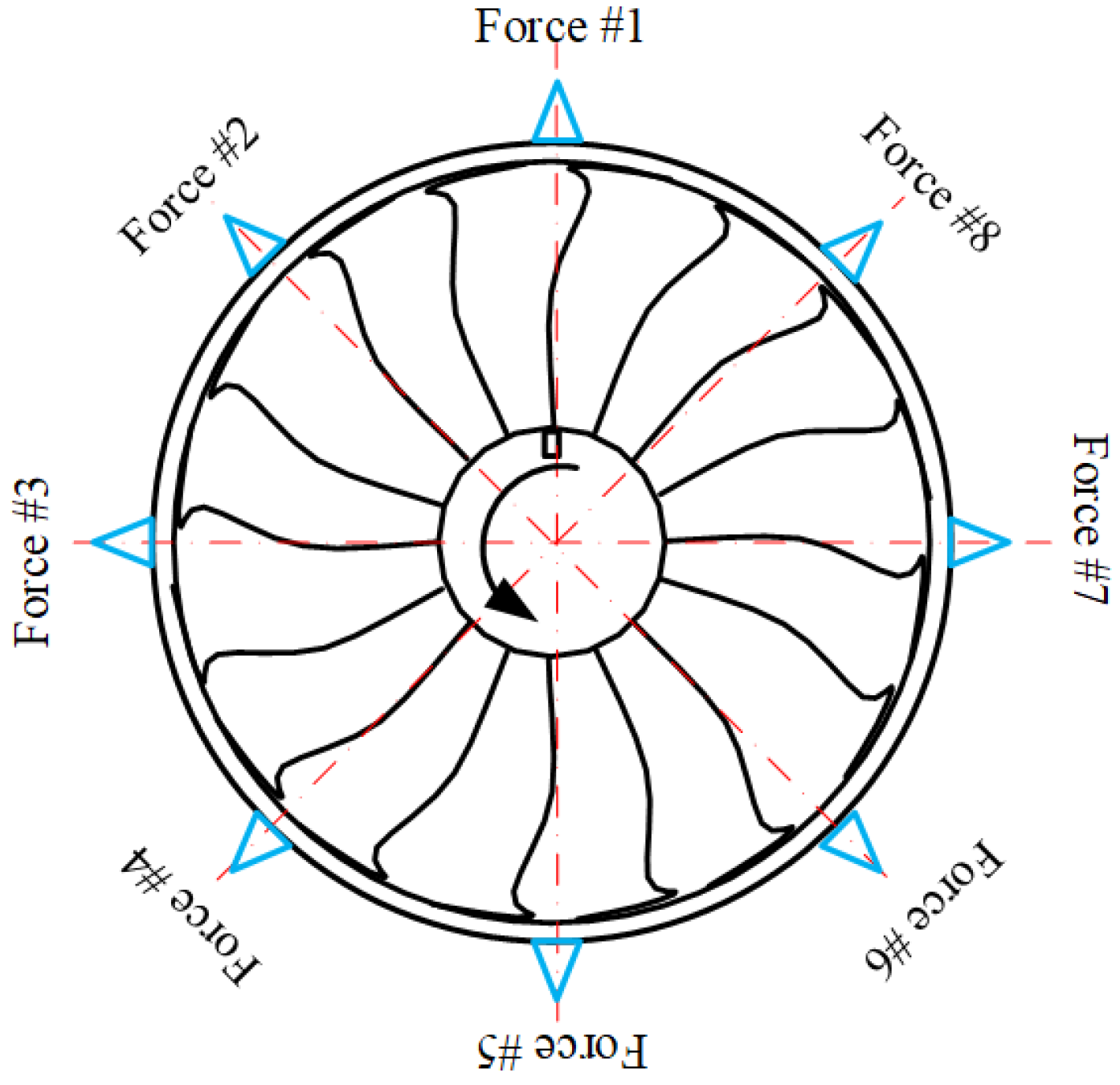
3.2. BTT Sampling Model

To study the sampling of the BTT method, the simulation program of BTT method is designed. The program can be decomposed into the following parts: simulation parameter setting, vibration displacement solving during blade rotation, trigger judgment of BTT probes and OPR probe, and signal recording. This subsection will mainly introduce the logic of sensor triggering judgment in the process of blade rotation, and at the same time, introduce the simulation method of sampling error and the blade installation angle error.

3.3. Solving the Vibration Response

To obtain the response of the blade under the excitation forces, the differential equations of the dynamics shown in Equation (11) are solved using a differential equation solution method such as the Runge–Kutta method or Newmark-βmethod. The vibration displacement $\mathbf{q}\left(t\right)$, vibration velocity $\dot{\mathbf{q}}\left(t\right)$, and vibration acceleration $\ddot{\mathbf{q}}\left(t\right)$ of the blades can be easily obtained based on this model. And velocity-based BTT (V-BTT) is also being taken as a new research direction [7,13,14,20], which is considered to be more favorable for obtaining high-precision blade vibration parameters.

Before the simulation starts, the values of the vibration displacement, velocity (first order derivative of displacement), and acceleration (second order derivative of displacement) vectors at the initial moment are set.

$$\ddot{\mathbf{q}}\left(t_0\right)=\dot{\mathbf{q}}\left(t_0\right)=\mathbf{q}\left(t_{\mathbf{0}}\right)=0$$

(26)

Set the step size of the numerical integration $f_{\mathrm{s}}$ according to the sampling frequency $f_{\mathrm{s}}$ of the sampling system. It is also the sampling period for digital sampling.

$$\mathrm{\Delta }{t}_{\mathrm{s}}={\displaystyle \frac{1}{f_{\mathrm{s}}}}$$

(27)

The relationship between sampling points and sampling moments is

$$t=t_0+{\displaystyle \frac{N}{f_{\mathrm{s}}}}$$

(28)

where N is the sequence of sampling periods, and it is also the data that is actually recorded during the actual sampling process. The ToA is obtained in the post-processing using Equation (28).

This certain step-size solution process exactly simulates the digital sampling process. That is, the recorded time is not continuous; each second is divided into time points. There is a definite interval $\mathrm{\Delta }{t}_{\mathrm{s}}$ between each time point.

For BTT sampling, the same sampling clock induces different resolution errors at different rotational speeds. The effect of sampling frequency on vibration displacement error is quantified in Equation (29).

$$\mathrm{\Delta }{q}_{\mathrm{m}\mathrm{a}\mathrm{x}}^{\mathrm{s}}={\displaystyle \frac{2\pi Rf}{f_{\mathrm{s}}}}={\displaystyle \frac{v}{f_{\mathrm{s}}}}$$

(29)

where $\mathrm{\Delta }{q}_{\mathrm{m}\mathrm{a}\mathrm{x}}^{\mathrm{s}}$ is the maximum error. f is the rotational speed of blade in Hz. v is the linear velocity of the blade tip. Equation (29) shows that the vibration displacement resolution is proportional to the linear velocity of the blade tip and inversely proportional to the clock frequency. Equation (29) can be used to calculate the resolution of the tip-timing sampling system. For example, when the vibration displacement accuracy is required to be less than 10 μm, if the linear velocity is 100 m/s, the sampling clock of the sampling system should be at least 10 MHz.

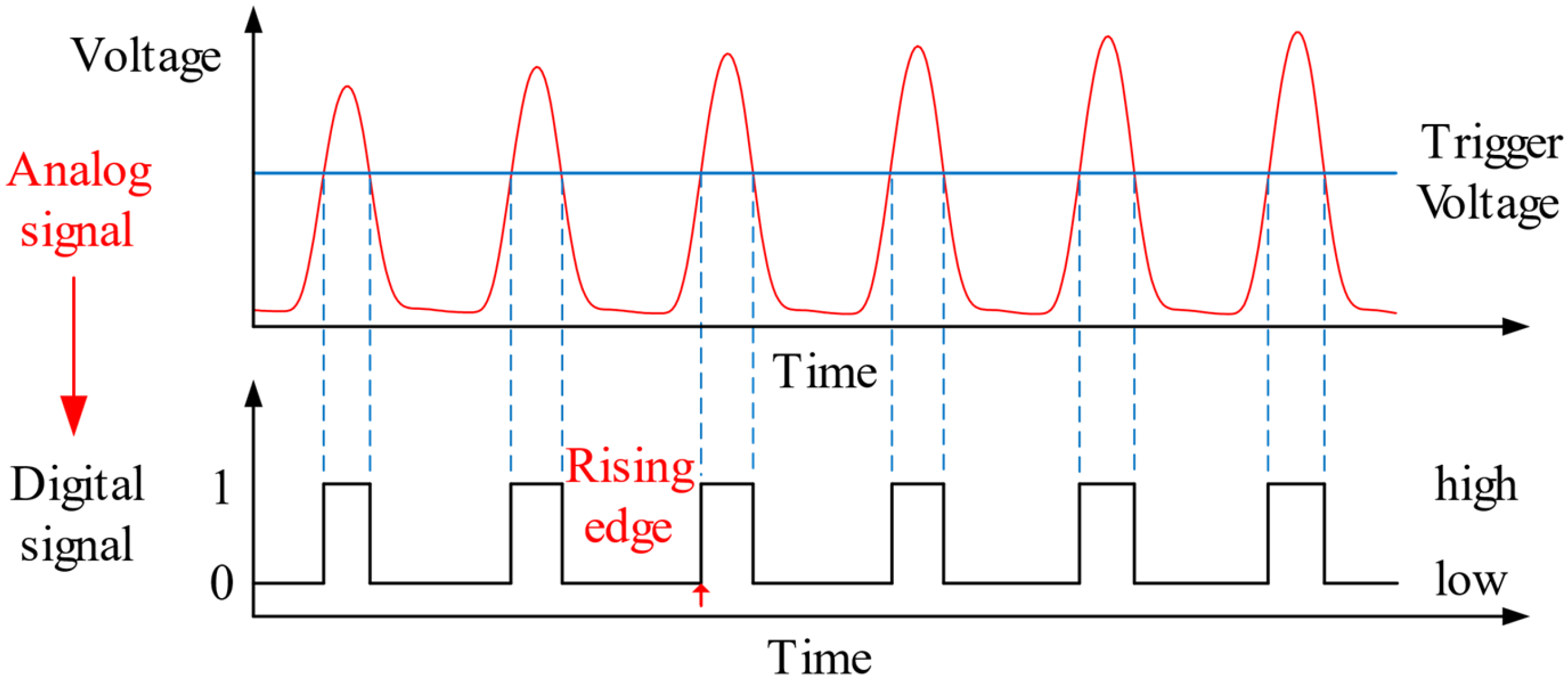
3.4. Probe Trigger and Probe Mounting Angle Error Simulation

The probes involved in the application of the BTT can be categorized into two types, i.e., the blade tip probes and OPR probe. In the simulation, these probes are essentially the same type, both recording the time of the blade or OPR passing through the probe in rotation. The difference is the number of trigger signals sampled in one revolution, which for the tip probe is the number of blades and for the OPR probe is the number of OPRs.

Figure 4 shows the trigger signal of the probe and the analog-to-digital conversion process of the test acquisition. The analog signal is the BTT arrival voltage signal collected by the fiber optic sensor-based acquisition system. To simulate the BTT sampling process, the following simulation program was constructed.

Figure 4. Sensor triggering and analog-to-digital conversion process.

Step 1: Probe layout setup

(1) Set each blade tip probe mounting angle ${\mathsf{\Phi }}_{(p,b)}$ according to Equation (8). The mounting angle of the probe is given by a sequence; to simulate the probe mounting angle error, you can define your own sequence of probe mounting angles (${\mathsf{\Phi }}_{\left(p,1\right)}^{\mathrm{i}\mathrm{d}\mathrm{e}\mathrm{a}\mathrm{l}}$) on demand, and add a certain deviation (${\mathsf{\Delta }\phi }_p$) to the probe mounting angle sequence in the simulation:

$${\mathsf{\Phi }}_{\left(p,1\right)}^{\mathrm{s}\mathrm{e}\mathrm{t}}={\mathsf{\Phi }}_{\left(p,1\right)}^{\mathrm{i}\mathrm{d}\mathrm{e}\mathrm{a}\mathrm{l}}+{\mathsf{\Delta }\phi }_p$$

(30)

(2) Setting the OPR probe mounting angle according to Equation (31).

$${\mathsf{\Phi }}_{\mathrm{O}\mathrm{P}\mathrm{R}\left(b\right)}={\mathsf{\Phi }}_{\mathrm{O}\mathrm{P}\mathrm{R}\left(1\right)}+\left(b-1\right){\displaystyle \frac{2\pi }{n_{\mathrm{b}}}}$$

(31)

where ${\mathsf{\Phi }}_{\mathrm{O}\mathrm{P}\mathrm{R}\left(b\right)}$ is the angular separation of the OPR probe from blade No. b.

Step 2: Analog-to-digital conversion

Referring to Equation (6), the rotation angle of the rotor blades accumulated at the moment t during the simulation of continuous sampling starting from t₀ is

$${\mathsf{\Psi }}_b(t)=2\pi \left({\displaystyle \frac{1}{2}}a{\left(t-t_0\right)}^2+f_0\left(t-t_0\right)\right)+{\displaystyle \frac{q_b\left(t\right)}{R\left(t\right)}}$$

(32)

where $q_b\left(t\right)$ is the vibrational displacement of blade No. b at time t.

The accumulated rotation angle of the OPR is

$${\mathsf{\Psi }}_{\mathrm{O}\mathrm{P}\mathrm{R}}(t)=2\pi \left({\displaystyle \frac{1}{2}}a{\left(t-t_0\right)}^2+f_0\left(t-t_0\right)\right)$$

(33)

The simulation might as well set the width of the angular domain of the blade or OPR to $w$°, and the signal captured by the probe when the blade or OPR passes through the probe to be 1, and the rest of the moments to be 0. Then, there are

$$\left\{\begin{array}{c}{P}_{\mathrm{R}}(t)=1\left(0\le \mathrm{mod} \left(\mathsf{\Psi }\left(t\right),2\pi \right)-{\mathsf{\Phi }}_{\left(b\right)}\le {\displaystyle \frac{w\pi }{180}}\right)\\ P_{\mathrm{R}}(t)=0\left({\displaystyle \frac{w\pi }{180}}<\mathrm{mod} \left(\mathsf{\Psi }\left(t\right),2\pi \right)-{\mathsf{\Phi }}_{\left(b\right)} \mathrm{o}\mathrm{r}\mathrm{mod} \left(\mathsf{\Psi }\left(t\right),2\pi \right)-{\mathsf{\Phi }}_{\left(b\right)}<0\right)\end{array}\right.$$

(34)

where $P_{\mathrm{R}}\left(t\right)$ is the probe response at time t. When $\mathsf{\Psi }\left(t\right)$ is denoted as the accumulated rotation angle of the blade ${\mathsf{\Psi }}_{\mathrm{b}}\left(t\right)$, ${\mathsf{\Phi }}_{\left(b\right)}$ denotes the angular interval from the tip probe No. p to the blade No. b. And when $\mathsf{\Psi }\left(t\right)$ is denoted as the accumulated rotation angle of the OPR ${\mathsf{\Psi }}_{\mathrm{O}\mathrm{P}\mathrm{R}}$, ${\mathsf{\Phi }}_{\left(b\right)}$ denotes the angular interval from the OPR probe to the blade No. b ${\mathsf{\Phi }}_{\mathrm{O}\mathrm{P}\mathrm{R}\left(b\right)}$.

In the simulation, the blade arriving at the probe (rising edge) can be used as the trigger signal.

The condition for an upward trigger is expressed as

$$P_{\mathrm{R}}\left(t\right)-P_{\mathrm{R}}\left(t-\mathrm{\Delta }{t}_{\mathrm{s}}\right)=1 \mathrm{o}\mathrm{r} P_{\mathrm{R}}\left(N\right)-P_{\mathrm{R}}(N-1)=1$$

(35)

3.5. Trigger Error Simulation

As shown in Figure 4, the actual sampling process determines the rising edge trigger by judging the magnitude of the voltage, and the trigger position will be approximate random with overrun or hysteresis due to various reasons. Based on the described probe-triggering judgment mechanism, this paper proposes a method to simulate the rising edge triggering error in the BTT sampling process.

$$N_{\mathrm{ToA}}=N+\mathrm{r}\mathrm{a}\mathrm{n}\mathrm{d}\mathrm{i}\left(-\mathrm{\Delta }{N}_{\mathrm{m}\mathrm{a}\mathrm{x}},N_{\mathrm{m}\mathrm{a}\mathrm{x}}\right)+N_{\mathrm{o}\mathrm{f}\mathrm{f}\mathrm{s}\mathrm{e}\mathrm{t}}$$

(36)

where $\mathrm{r}\mathrm{a}\mathrm{n}\mathrm{d}\mathrm{i}\left(-\mathrm{\Delta }{N}_{\mathrm{m}\mathrm{a}\mathrm{x}},N_{\mathrm{m}\mathrm{a}\mathrm{x}}\right)$ is a random integer in the generated interval $[-\mathrm{\Delta }{N}_{\mathrm{m}\mathrm{a}\mathrm{x}},N_{\mathrm{m}\mathrm{a}\mathrm{x}}]$. $\mathrm{\Delta }{N}_{\mathrm{m}\mathrm{a}\mathrm{x}}$ is the maximum sampling interval number of trigger error (integer). $N_{\mathrm{o}\mathrm{f}\mathrm{f}\mathrm{s}\mathrm{e}\mathrm{t}}$ is the number of sampling intervals (integer) in advance or delay, which is used to simulate the error caused by trigger voltage selection, with advance being positive and delay being negative.

The amount of error introduced by the sampling error on the vibration displacement is

$$\mathsf{\Delta }q=2\pi R{f}_{\left(n\right)}{\displaystyle \frac{\mathrm{r}\mathrm{a}\mathrm{n}\mathrm{d}\mathrm{i}\left(-\mathrm{\Delta }{N}_{\mathrm{m}\mathrm{a}\mathrm{x}},N_{\mathrm{m}\mathrm{a}\mathrm{x}}\right)+N_{\mathrm{o}\mathrm{f}\mathrm{f}\mathrm{s}\mathrm{e}\mathrm{t}}}{f_{\mathrm{s}}}}={\displaystyle \frac{v_{\left(n\right)}}{f_{\mathrm{s}}}}\left(\mathrm{r}\mathrm{a}\mathrm{n}\mathrm{d}\mathrm{i}\left(-\mathrm{\Delta }{N}_{\mathrm{m}\mathrm{a}\mathrm{x}},N_{\mathrm{m}\mathrm{a}\mathrm{x}}\right)+N_{\mathrm{o}\mathrm{f}\mathrm{f}\mathrm{s}\mathrm{e}\mathrm{t}}\right)$$

(37)

3.6. Blade Mounting Angle Error Simulation

Due to processing errors and other reasons, the actual blade cannot be completely uniformly arranged on the blade disk, so Equation (22) only represents the ideal case of the phase delay of the blade; if you consider the blade mounting angle error, Equation (22) needs to be rewritten:

$${\phi }_b={\displaystyle \frac{2\pi (b-1)}{n_{\mathrm{b}}}}+{\mathrm{\Delta }\phi }_{\mathrm{m}\mathrm{a}\mathrm{x}}\mathrm{r}\mathrm{a}\mathrm{n}\mathrm{d}(\ast )$$

(38)

where ${\mathrm{\Delta }\phi }_{\mathrm{m}\mathrm{a}\mathrm{x}}$ the maximum angular error.

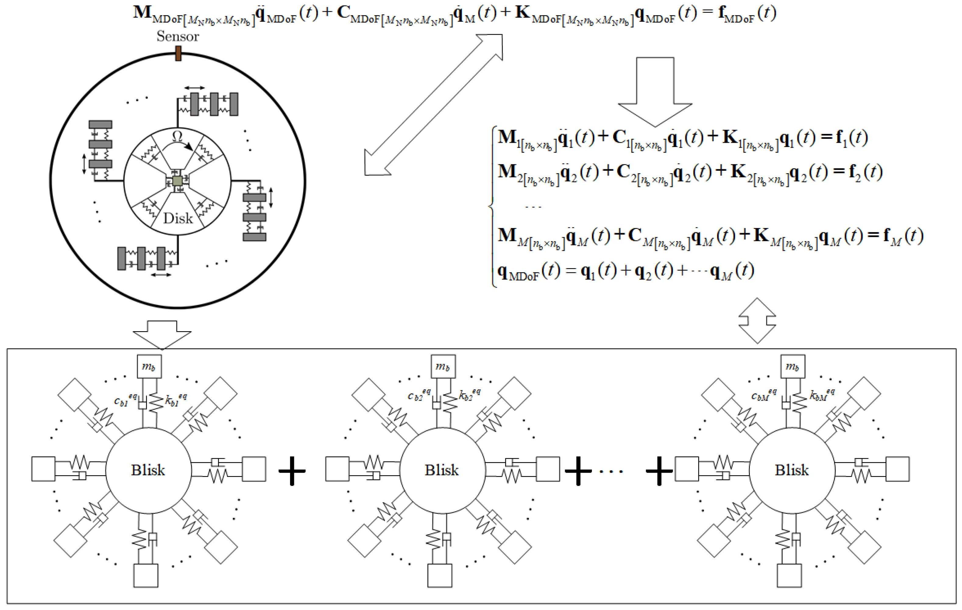
3.7. Multi-Harmonic Vibration Model

In most cases, it is sufficient to verify the validity of the BTT method based on a SDoF blade disk model. If the multi-harmonic vibration of the blade needs to be investigated, a more complex model, such as a MDoF model, needs to be constructed [6]. However, the construction and solution of the MDoF model is very challenging. For this reason, this paper proposes a simpler and more efficient method to realize the simulation of multi-modal blade vibration and BTT sampling simulation.

In the presence of multi-mode, the blade-tip vibration displacement response is the sum of harmonic signals of different frequencies [14]. The multimodal vibration displacement of the blade can be expressed as

$$q_{\mathrm{MDoF}}(t)=\sum _{M=1}^{M_{\mathrm{N}}}\left[A_M\sin (2\pi {\omega }_M^{\mathrm{n}}t)+B_M\cos (2\pi {\omega }_M^{\mathrm{n}}t)+C_M\right]=\sum _{M=1}^{M_{\mathrm{N}}}{q}_M\left(t\right)$$

(39)

where $M_{\mathrm{N}}$ is the number of modes. The subscript M denotes the M-th mode. A, B, and C are the parameters determined by the phase and amplitude coefficients of vibration q(t).

From Equation (39), the multimodal vibration displacement can actually be decomposed into a superposition of multiple SDoF vibrations (with corresponding natural frequencies, amplitudes, and phases) (Figure 5). Therefore, the simplest and most effective multimodal simulation only requires the construction of multiple SDoF blade models. Based on the dynamic equations shown in Equation (11), the vibration displacements of modes are obtained independently. And the superposition of each SDoF vibration displacement at the same moment can be equated to the multimodal vibration displacement. This solution allows the matrix equations of order $M_{\mathrm{N}}{n}_{\mathrm{b}}\times M_{\mathrm{N}}{n}_{\mathrm{b}}$ (Equation (40)), which need to be solved for a MDoF model, to be solved for $M_{\mathrm{N}}$ matrix equations of order $n_{\mathrm{b}}\times n_{\mathrm{b}}$ (Equation (41)). This greatly reduces the modeling difficulty as well as the computational difficulty.

$${{\mathbf{M}}_{\mathrm{MDoF}}}_{\left[M_{\mathrm{N}}{n}_{\mathrm{b}}\times M_{\mathrm{N}}{n}_{\mathrm{b}}\right]}{\ddot{\mathbf{q}}}_{\mathrm{MDoF}}(t)+{{\mathbf{C}}_{\mathrm{MDoF}}}_{\left[M_{\mathrm{N}}{n}_{\mathrm{b}}\times M_{\mathrm{N}}{n}_{\mathrm{b}}\right]}{\dot{\mathbf{q}}}_M(t)+{{\mathbf{K}}_{\mathrm{MDoF}}}_{\left[M_{\mathrm{N}}{n}_{\mathrm{b}}\times M_{\mathrm{N}}{n}_{\mathrm{b}}\right]}{\mathbf{q}}_{\mathrm{MDoF}}(t)={\mathbf{f}}_{\mathrm{MDoF}}(t)$$

(40)

$$\begin{array}{c}{{\mathbf{M}}_M}_{\left[n_{\mathrm{b}}\times n_{\mathrm{b}}\right]}{\ddot{\mathbf{q}}}_M(t)+{{\mathbf{C}}_M}_{\left[n_{\mathrm{b}}\times n_{\mathrm{b}}\right]}{\dot{\mathbf{q}}}_M(t)+{{\mathbf{K}}_M}_{\left[n_{\mathrm{b}}\times n_{\mathrm{b}}\right]}{\mathbf{q}}_M(t)={\mathbf{f}}_M(t)\\ \left(M=\mathrm{1,2},\dots {,M}_{\mathrm{N}}\right)\end{array}$$

(41)

Figure 5. Multi-modal decoupling.

For each mode, there is

$$m_M^{\mathrm{eq}}=m\left(M=\mathrm{1,2},\dots ,M_{\mathrm{N}}\right)$$

(42)

where m^eq is equivalent mass. Therefore, the mass matrix of each equivalent mode is consistent with Equation (12).

The equivalent stiffness $k_M^{\mathrm{eq}}$ of the blade in each mode is calculated based on Equation (43).

$$k_M^{\mathrm{eq}}={\left(2\pi {\omega }_M^{\mathrm{n}}\right)}^{2}m$$

(43)

The maximum vibration displacement of the blade can be calculated from Equation (44).

$$x_{\mathrm{m}\mathrm{a}\mathrm{x}}={\displaystyle \frac{F_{\mathrm{m}\mathrm{a}\mathrm{x}}}{2\mathsf{\xi }k}}$$

(44)

The vibration amplitude of each mode can be realized by setting the amplitude of the excitation force and the equivalent damping ratio of each mode.

The vibration displacements, vibration velocities and vibration accelerations used for BTT sampling simulations are

$$\left\{\begin{array}{c}{\mathbf{q}}_{\mathrm{MDoF}}\left(t\right)={\mathbf{q}}_1\left(t\right)+{\mathbf{q}}_2\left(t\right)+\cdots +{\mathbf{q}}_M\left(t\right)\\ {\dot{\mathbf{q}}}_{\mathrm{MDoF}}\left(t\right)={\dot{\mathbf{q}}}_1\left(t\right)+{\dot{\mathit{q}}}_2\left(t\right)+\cdots +{\dot{\mathbf{q}}}_M\left(t\right)\\ {\ddot{\mathbf{q}}}_{\mathrm{MDoF}}\left(t\right)={\ddot{\mathbf{q}}}_1\left(t\right)+{\ddot{\mathbf{q}}}_2\left(t\right)+\cdots +{\ddot{\mathbf{q}}}_M\left(t\right)\end{array}\right.$$

(45)

4. Comparison of Simulation and Experimental Results

We have completed the programming of the rotating blade vibration and BTT sampling system simulator based on Fortran. Repeated definition of the model and simulation is achieved by reading the setup parameter file. The parameters that can be modified include blade parameters (single-mode or multi-mode equivalent model, degree of mass mistuning, blade disk size, etc.), number of probe, actual probe mounting angle, probe-triggering error, number of blades, actual blade mounting angle, simulation time, numerical sampling frequency, rotational process variables (constant speed, variable speed, rotational speed fluctuation, etc.), number and type of excitation forces, and so on. The final simulator can output the full simulation process of each blade’s vibration displacement, vibration velocity, the ToA collected by each probe, and the actual vibration displacement and other data files. In this section, the validity of the simulation model will be verified for some cases, and it can also be used as a validation case for the readers to build their own simulation models.

4.1. Single-Mode Vibration Simulation

To verify the correctness of the proposed simulation model, the simulation results are compared with the theoretical analysis in this section. Table 1 shows the parameter settings of the blade model simulation used in this section.

Table 1. Blade model parameters—series I.

Mass of Blades m (Unit: kg)	$\mathbf{Nature} \mathbf{Frequency} {\mathit{\omega }}^{\mathbf{n}}$ (Unit: Hz)	$\mathbf{Damping} \mathbf{Ratio} \mathsf{\xi }$	Blade Number nb	Radius of Blade Disk R (Unit: m)	$\mathbf{Maximum} \mathbf{Mass} \mathbf{Mistuning} {\mathit{\delta }}_{\mathbf{m}\mathbf{a}\mathbf{x}}$ (Unit: kg)	Sampling Frequency ${\mathit{f}}_{\mathbf{s}}$ (Unit: MHz)
0.05	2000	0.001	32	0.05	0.05 × m	5

The stiffness of the blade can be calculated using Equation (46):

$$k={\left(2\pi {\omega }^{\mathrm{n}}\right)}^{2}m$$

(46)

The damping of the blade can be calculated using Equation (47):

$$c=2\mathsf{\xi }\sqrt{mk}$$

(47)

They are calculated to obtain k = 7,895,683.52 N/m and c = 1.26 N∙s/m.

Three tip probes and one OPR probe were set up in the simulation. The installation angle of the OPR probe is set to 1°, and the 3 tip probes are arranged at angles of 0°, 6°, and 12° with respect to the OPR probe.

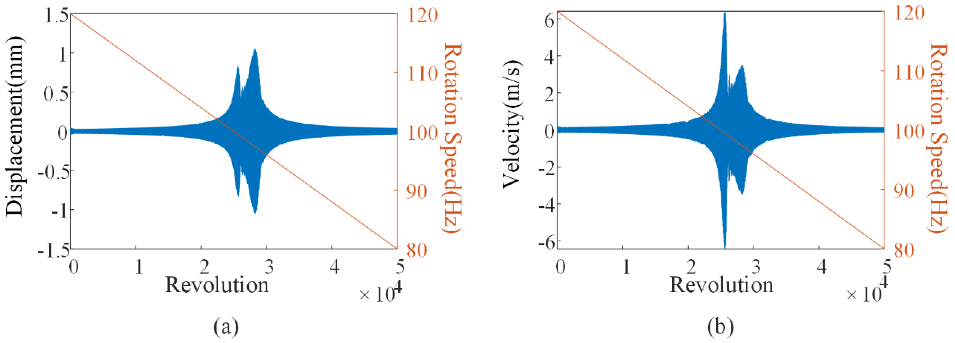
4.1.1. Simulation of Synchronous Vibration Based on Sinusoidal Excitation Force

To simulate the synchronous vibration of the blade, the excitation force and other parameters of the model are used (shown in Table 2). Only one excitation force case is considered here.

Table 2. Exciting force and simulation parameter setting—series I.

$\mathbf{Force} \mathbf{Amplitude} {\mathit{F}}_{\mathbf{max} \left(\mathit{b}\right)}$ (Unite: N)	$\mathbf{Engine} \mathbf{Order} {\mathit{n}}^{\mathbf{EO}}$	Start Frequency (Unite: Hz)	End Frequency (Unite: Hz)	Simulation Time (Unite: s)
20	20	95	105	10

The calculation yields $x_{\mathrm{m}\mathrm{a}\mathrm{x}}$ = 1.2665 mm. If the blade vibration simulation is carried out at a constant speed of 100 Hz, the results obtained are shown in Figure 6, and the amplitude of blade vibration after solving the stabilization is 1.265 × 10⁻³ m, which is basically the same as that obtained by Equation (44), which illustrates the accuracy of the model solving.

Figure 6. Simulation results of blade synchronous vibration at constant speed.

Figure 7 shows the vibration displacement of a blade obtained from the simulation; the maximum vibration amplitude is 1.18 × 10⁻³ m as black dot shows. Compared with the results in Equation (44), it is small, which is due to the process of speed up. Usually, the faster the rate of speed up, the smaller the maximum amplitude of vibration.

Figure 7. The relationship between vibration displacement and rotational speed of a blade.

Figure 8 shows the vibration displacement obtained from the simulated sampling.

Figure 8. Synchronous vibration simulation results of BTT.

4.1.2. Simulation of Synchronous Vibration Based on Multi-Source Square Wave Excitation Force

To provide a simulation case of the multi-source square wave excitation force model, the following simulation parameters are set (Table 3). The rate of degradation of the sweeping process is 10 Hz/s.

Table 3. Square wave excitation force model parameters—series I.

$\mathbf{Amplitude} \mathbf{of} \mathbf{a} \mathbf{Single} \mathbf{Force} {\mathit{A}}_{\mathit{i}}$ (Unit: N)	$\mathbf{Number} \mathbf{of} \mathbf{Force} {\mathit{N}}_{\mathbf{F}}$	Start Frequency (Unite: Hz)	End Frequency (Unite: Hz)	Simulation Time (Unite: s)
20	20	310	10	30

Figure 9 is the results of BTT for all blades. Due to the mass mistuning setup, the vibration center frequency of each blade has some differences.

Figure 9. Results of BTT for all blades.

The vibration displacement response of a blade under the set excitation force is shown in Figure 10, which excites several synchronous resonance intervals.

Figure 10. Vibration response of a blade.

Figure 11 shows the vibration displacements of the blade as it passes through each probe. Figure 11a shows the vibration displacements solved in the simulation, i.e., the actual blade vibration values, and Figure 11b shows the blade vibration displacements obtained by processing the blade arrival times from the simulation using the BTT method. Meanwhile, Figure 11b shows that the measurement error due to sampling frequency increases as the rotational speed increases.

Figure 11. Blade vibration collected by BTT method. (a) True value of the blade vibration displacement when the probe is triggered. (b) Vibration displacement of the blade obtained using BTT analysis.

In this case, when the speed is 300 Hz, the linear speed is 94.25 m/s, and $\mathsf{\Delta }{q}_{\mathrm{m}\mathrm{a}\mathrm{x}}^{\mathrm{s}}$ = 18.85 μm is calculated. As shown in Figure 12, in the vicinity of 300 Hz, the error between the measured value (the maximum value is indicated by a black square) and the true value is less than that of the Equation (29) calculation result without adding other noise, which shows that the simulation model can simulate the system sampling error at different sampling frequencies.

Figure 12. Comparison of real value and measured value near 300 Hz (5 MHz).

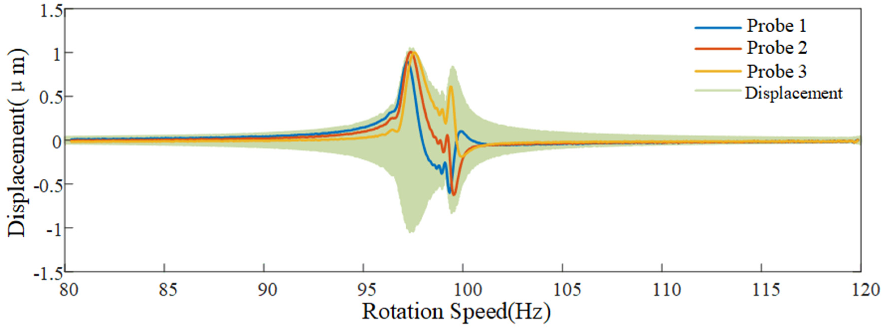
4.1.3. Effect of Trigger Position Error

The trigger point error simulation is performed using the same model parameters and simulation parameters as Section 4.1.2, and the sampling frequency is changed to 20 MHz. Without considering the trigger point error, the vibration displacement results of blade are shown in Figure 13. Compared with the results obtained at a sampling frequency of 5 MHz (Figure 11b), the results shown in Figure 13 maintain a lower level of measurement error of blade vibration displacement at high speed (line speed) due to the improved sampling frequency. This shows that increasing the sampling clock frequency can significantly reduce the measurement uncertainty caused by the resolution of the sampling time point.

Figure 13. Blade vibration response obtained by BTT probe (20 MHz).

From Equation (29), $\mathsf{\Delta }{q}_{\mathrm{m}\mathrm{a}\mathrm{x}}^{\mathrm{s}}$ = 4.7125 μm. As shown in Figure 14, the maximum difference between the measured and true values near 300 Hz is in accordance with Equation (29).

Figure 14. Real value and measured value near 300 Hz (20 MHz).

The trigger error of the OPR probe is set according to Equation (36), and in general, the arrival time error caused by the trigger position error of the OPR probe is within 1 μm. When the sampling clock frequency of the sampling system is set to 20 MHz, the moment difference between the two time points Δt_s = 1/fs = 1/20∙10⁻⁶ s.

Therefore, set ΔN_max = 5 and N_offset = 2. Figure 15 shows the blade vibration response with the OPR probe trigger errors, and it can be seen that the blade vibration displacement measurement error due to the OPR probe trigger errors grows linearly as the rotational speed rises. Figure 16 shows the vibration displacement measurement error of probe 1. The measurement error is between −23 µm and 32 µm at around 300 Hz. If calculated using Equation (37), the range of the error is between −14.14 μm and 33 μm, and the measurement results are basically as expected.

Figure 15. Blade vibration response obtained by BTT method in the presence of trigger error of the OPR probe.

Figure 16. Measurement error of BTT method.

Therefore, the error caused by the selection of the trigger position is not negligible. The upper limit of the accuracy of the BTT method still depends mainly on the sampling clock frequency of the system. In order to reach this upper limit, a more in-depth study of the BTT method is needed, including the selection of the trigger point, the design of the sensor, and the displacement calculation method.

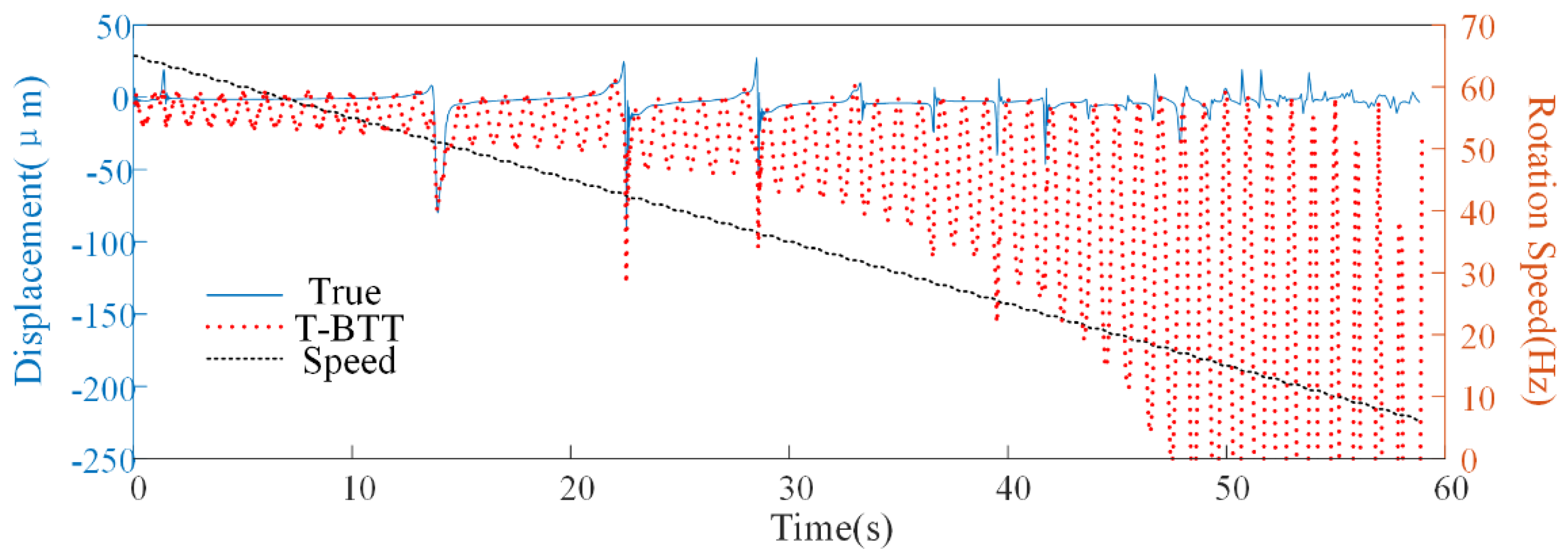
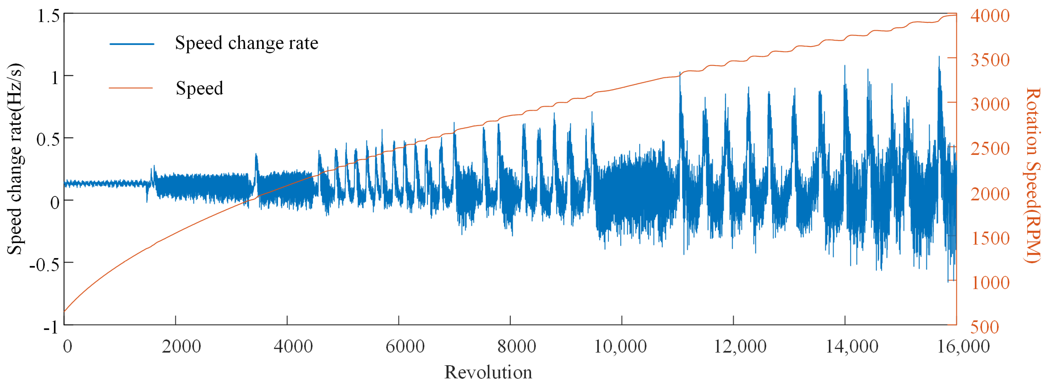
4.1.4. Speed Fluctuation

Simulation with sinusoidal speed fluctuation during speed reduction is carried out using the simulation parameters of Table 4. The sinusoidal speed fluctuation rate is $\cos (2\pi t)$ Hz/s with a period of 1 s.

Table 4. Square wave excitation force model parameters—seriese II.

$\mathbf{Amplitude} \mathbf{of} \mathbf{a} \mathbf{Single} \mathbf{Force} {\mathit{A}}_{\mathit{i}}$ (Unit: N)	$\mathbf{Number} \mathbf{of} \mathbf{Force} {\mathit{N}}_{\mathbf{F}}$	Start Frequency (Unite: Hz)	End Frequency (Unite: Hz)	Simulation Time (Unite: s)
20	20	310	10	30

Therefore, the rotational speed equation is

$$\mathsf{\Omega }(t)=-t+65+{\displaystyle \frac{\sin (2\pi t)}{2\pi }}$$

(48)

And the rotational equation is

$${\mathsf{\Phi }}_1(t)=2\pi {\int }_0^t\mathsf{\Omega }\left(t\right)\mathrm{d}t\begin{array}{c}=\end{array}\pi t^2+130\pi t-{\displaystyle \frac{\cos \left(2\pi t\right)-1}{2\pi }}$$

(49)

Based on the ToA obtained from the simulation, the rotational speed fluctuation calculated using SG-BTT [21] is shown in Figure 17.

Figure 17. RPM vs. speed change rate (simulation).

The vibration displacements obtained using T-BTT and the true values of all the blades are shown in Figure 18. The different positions of the blades are affected by speed fluctuations differently. The error of the blade No. 1, which is closest to the OPR, is the smallest. And the errors basically show a tendency to increase with the increase in the distance from the OPR.

Figure 18. Vibration displacement of all blades. (a) Real blade vibration; (b) T-BTT.

The comparison of the vibration displacements of blades No. 2 and No. 16 obtained by T-BTT method with the true values are shown in Figure 19 and Figure 20 below. The obtained vibration displacements are significantly different from the true values, and the lower the rotational speed, the greater the influence of rotational speed fluctuations, which includes the influence of sinusoidal fluctuations, as well as the deceleration processes. Therefore, in this case, the T-BTT cannot be used properly and the BTT method, which takes into account the influence of the rotational speed fluctuations, needs to be used.

Figure 19. Vibration displacement of blade No. 2 (simulation).

Figure 20. Vibration displacement of blade No. 16 (simulation).

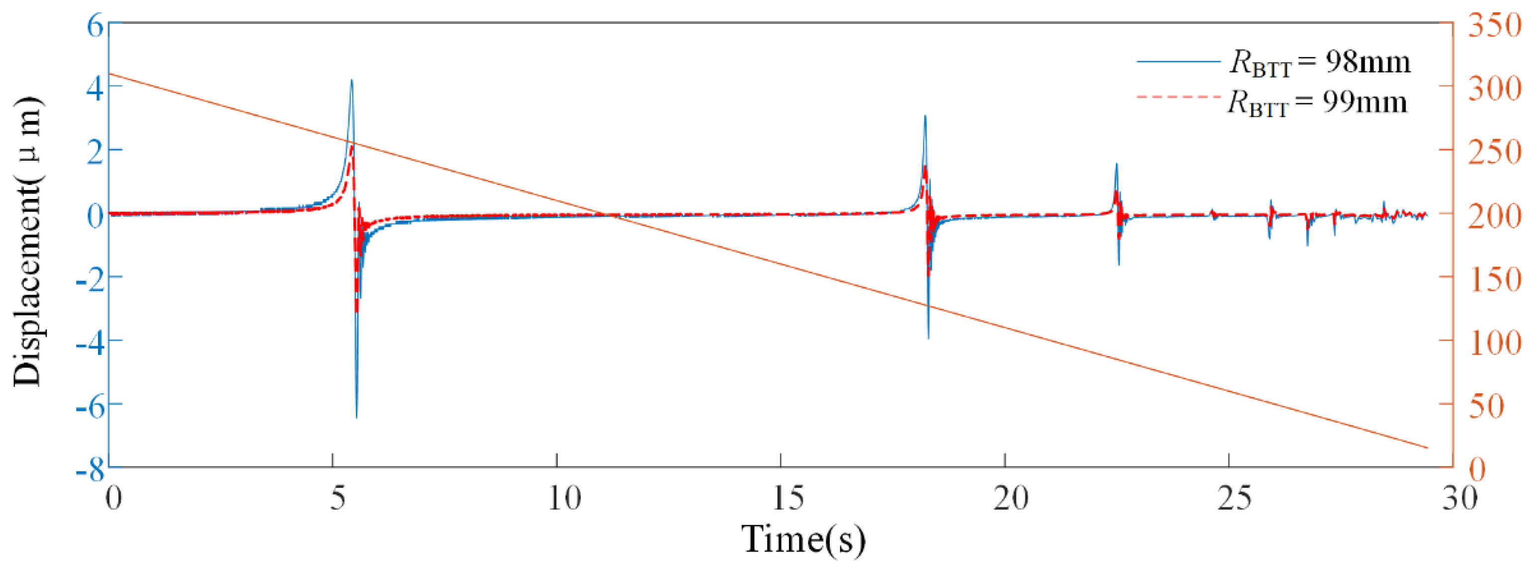
4.1.5. Effect of Changes in Blade Radius

The simulation results in Section 4.1.3 are used here without considering the triggering error. In the BTT analysis, the diameter of the blade is set to 99 mm and 98 mm, to simulate the impact on the BTT analysis results when the BTC is reduced by 0.5 mm and 1 mm (the blade is elongated by 1 mm and 2 mm in rotation), respectively. Figure 21 shows the relative error between the vibration displacement calculation results of blade No.1 in the above two cases and the results with the diameter set to 100 mm. Combined with Figure 13, the effect of BTC on the BTT results increases with the deformation of the blade. Therefore, simultaneous monitoring of BTT and BTC is necessary, especially for large rotating machines with larger blade diameters and more intense vibrations, and the influence of BTC on BTT measurements is more pronounced.

Figure 21. The displacements relative error of the blade 1 obtained by probe 1.

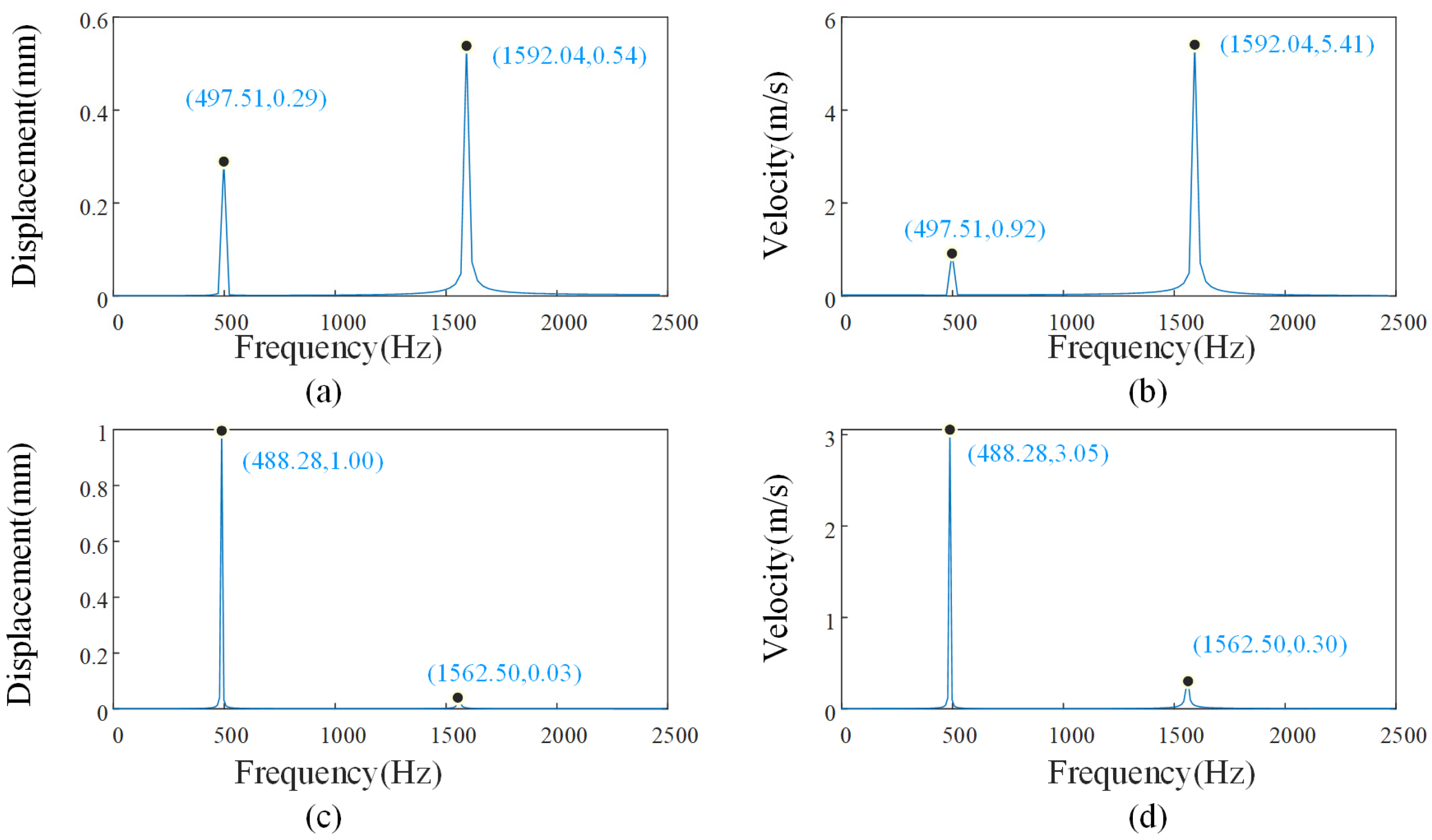
4.2. Multi-Harmonic Vibration Simulation

The multi-harmonic vibration of the blade is simulated based on the parameters in Table 5, which simulates vibration response of the two blade modes.

Table 5. Blade model parameters—seriese II.

Mass of Blades m (Unit: kg)	Blade Number nb	Radius of Blade Disk R (Unit: m)	$\mathbf{Maximum} \mathbf{Mass} \mathbf{Mistuning} {\mathit{\delta }}_{\mathbf{m}\mathbf{a}\mathbf{x}}$ (Unit: kg)	Sampling Frequency ${\mathit{f}}_{\mathbf{s}}$ (Unit: MHz)	Mode 1		Mode 2
					$\mathbf{Nature} \mathbf{Frequency} {\mathit{\omega }}_1^{\mathbf{n}}$ (Unit: Hz)	$\mathbf{Damping} \mathbf{Ratio} {\mathsf{\xi }}_1$	$\mathbf{Nature} \mathbf{Frequency} {\mathit{\omega }}_2^{\mathbf{n}}$ (Unit: Hz)	$\mathbf{Damping} \mathbf{Ratio} {\mathsf{\xi }}_2$
0.05	32	0.05	0.03 × m	5	486	0.005	1587	0.0015

Using the sinusoidal excitation force described in Equation (21), the parameters are shown in Table 6.

Table 6. Exciting force and simulation parameter setting—seriese II.

$\mathbf{Force} \mathbf{Amplitude} {\mathit{F}}_{\mathbf{max} \left(\mathit{b}\right)1}$ (Unite: N)	$\mathbf{Engine} \mathbf{Order} {\mathit{n}}_1^{\mathbf{EO}}$	$\mathbf{Force} \mathbf{Amplitude} {\mathit{F}}_{\mathbf{max} \left(\mathit{b}\right)2}$ (Unite: N)	$\mathbf{Engine} \mathbf{Order} {\mathit{n}}_2^{\mathbf{EO}}$	Start Frequency (Unite: Hz)	End Frequency (Unite: Hz)	Simulation Time (Unite: s)
10	5	20	16	120	80	20

The excitation force is shown in Equation (21), and the parameters are shown in Table 6.

The ToA, measured by the three probes, was processed using T-BTT to obtain the blade vibration displacement. The displacements of blade No. 16 as it passes through the probes are shown in Figure 22, which is significantly different to the SDoF model.

Figure 22. The displacements of blade 16, obtained by probes.

The vibration displacement and vibration velocity of blade No.16, obtained from the simulation, are resampled with sampling frequency of 5000 Hz, and the results are shown in Figure 23. An FFT analysis of vibration displacement and vibration velocity near the two peaks (25,550 th rev to 25,750 th rev and 28,000 th rev to 28,511 th rev) is shown in Figure 24.

Figure 23. Tip vibration displacement and vibration velocity of blade No. 16. (a)Vibration displacement. (b) Vibration velocity.

Figure 24. Spectral analysis results. (a) and (b) 25,550 th rev to 25,750 th rev (99.60 Hz to 99.36 Hz); (c) and (d) 28,000 th rev to 28,511 th rev (97.60 Hz to 97.19 Hz).

The relationship between the amplitude obtained by V-BTT $A_M^{\mathrm{V}}$ [14] and the amplitude obtained by D-BTT $A_M^{\mathrm{d}}$ is in accordance with

$${\displaystyle \frac{A_M^{\mathrm{V}}}{A_M^{\mathrm{d}}}}=2\pi {\omega }_M^{\mathrm{n}}$$

(50)

Based on the amplitude data shown in Figure 24, ${\omega }_1^{\mathrm{n}}=485 \mathrm{H}\mathrm{z}$ and ${\omega }_2^{\mathrm{n}}=1594 \mathrm{H}\mathrm{z}$ can be solved, which are basically consistent with the spectrum results and simulation settings. The correctness of the present model and solution is further verified.

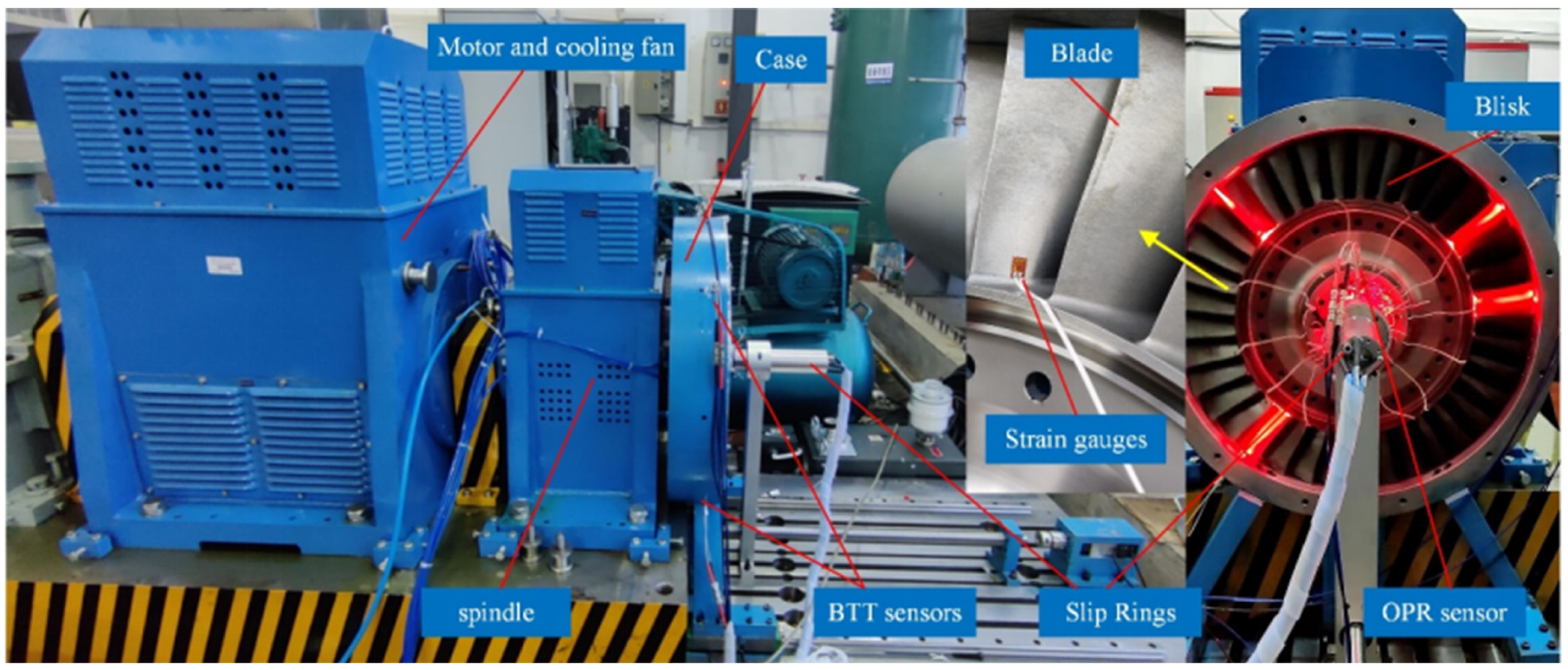
4.3. Comparison with Test Results

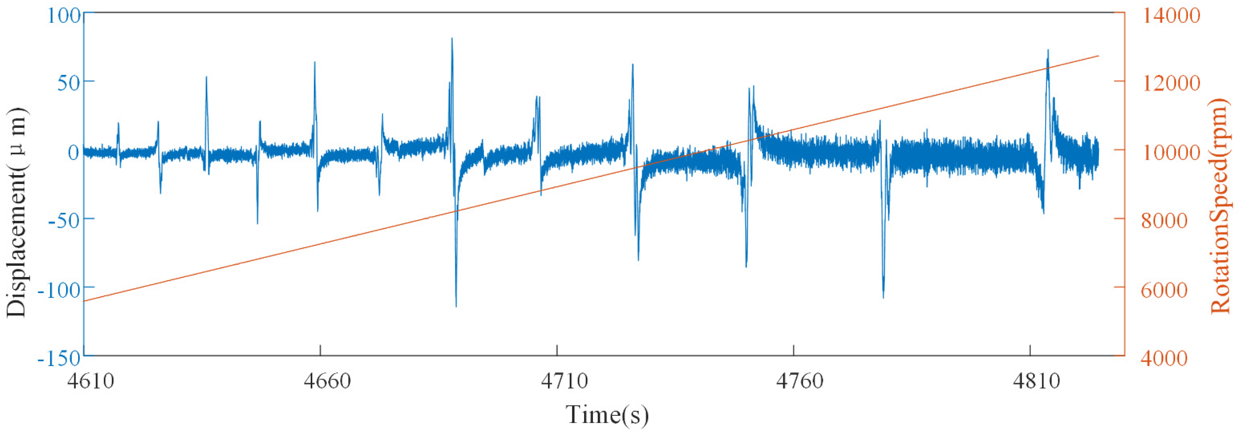
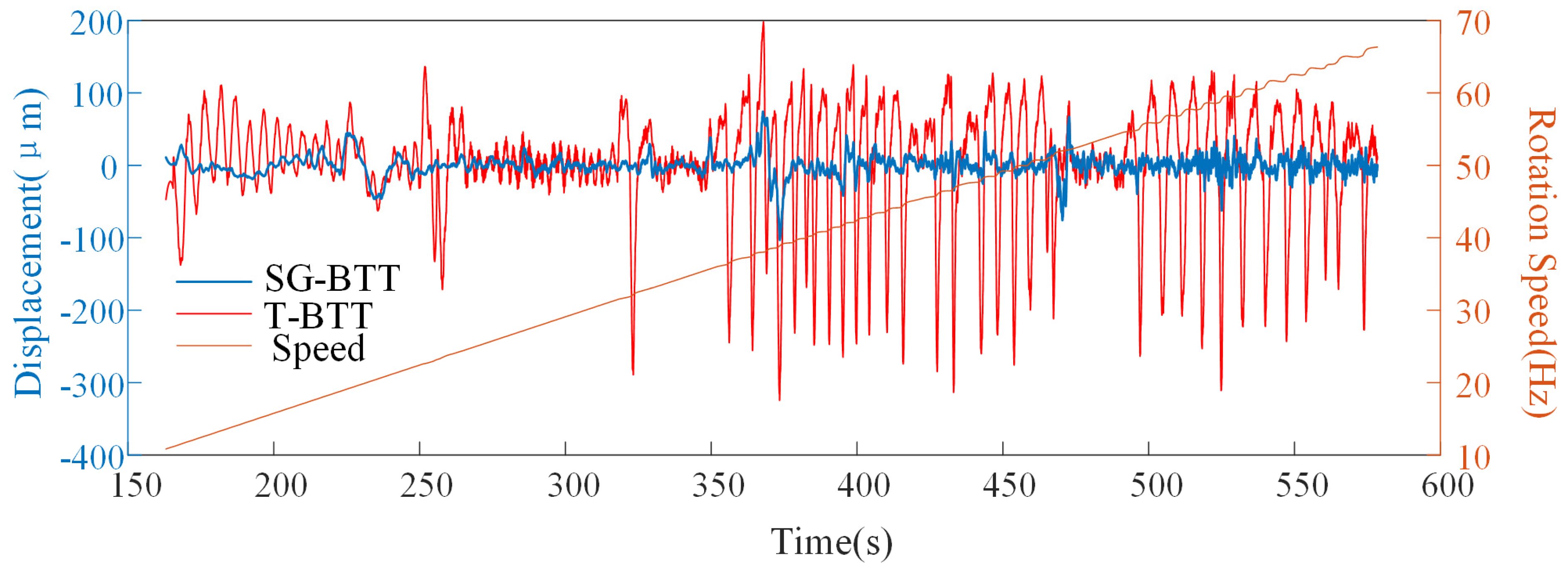
4.3.1. The Acceleration Process Verification

To compare the proposed simulation model with the actual test bench, a high-speed twist blade test bench (Figure 25) is used to carry out experimental research. The high-speed twist blade test bench mainly consists of a base, a stand (with a built-in motor), an operating platform, a torsion blade disk, a shroud, an air grill, and other components. The monolithic blade disk has a diameter of 138 mm and a total of 32 blades. The simple structure of this test bench allows for relatively clear uncertainty and high-quality signals to be obtained during BTT sampling.

Figure 25. High-speed twist blade test bench. 1. Blade disk. 2. Flow guide portal. 3. BTT sensor. 4. Vents. 5. Operating platform. 6. Support (motor). 7. Base. 8. BTC sensor. 9. Shaft displacement sensor.

The actual BTT sampling involves more uncertainties, and the blade excitation force model based on the existing simulation model cannot fully simulate the actual vibration situation. The model focuses on qualitative validation of the BTT algorithm’s sensitivity to vibration modes and uncertainties, which are scale-independent phenomena. The comparison in this section mainly focuses on the qualitative analysis of the simulation phenomenon. Therefore, the main role of the analog simulation carried out in this paper in comparison with experiments is to reveal the existing experimental phenomena associated with various uncertainties and to provide a more effective simulator for the development and validation of new algorithms.

The rotor is accelerated from 5800 rpm to 13,000 rpm, and the tip displacement is calculated by the BTT method, as shown in Figure 26. It shows the same phenomena as Figure 11; that is, as the speed increases, the measurement error also increases.

Figure 26. Displacement calculated by the BTT method.

4.3.2. Verification of Speed Fluctuation

A turbine blade test bench is built to perform some vibration tests on the compressor blades. The main part of the test bench is mainly composed of motor and spindle. A turbine engine full-size integral compressor blisk is mounted on the spindle. The diameter of the blisk is 553 mm. The number of blades is 37. Strain gauges are attached to the blade and a slip ring is mounted on the output shaft end. The fiber optic type of BTT sensor is mounted on the blade protection casing. The OPR probe is at the output shaft end, again with a fiber optic sensor. Figure 27 shows the main part of the test bench. In addition to the parts visible in the diagram, the test system includes the control system, the lubrication system, and the piping. The structure of this experimental bench is relatively complex, capable of complex uncertainty situations, and able to give the reader a deeper understanding of the BTT sampled signals during practical applications.

Figure 27. Compressor blade test bench.

In one of the experiments, the rotational speed showed a significant periodic fluctuation. The rotational speed and the change rate of rotational speed calculated using SG-BTT are shown in Figure 28.

Figure 28. RPM vs. speed change rate.

The vibration displacements of all the blades obtained by using the BTT method considering the effect of speed fluctuation and T-BTT processing the ToA of probe No. 1 are shown in Figure 29. There is a significant difference in the vibration displacements obtained by T-BTT in the low-speed region, and this difference is consistent with the simulation results (Figure 18). In contrast, the BTT method considering the effect of rotational speed fluctuation does not have this difference, and the overall trend of vibration displacements of individual blades is consistent.

Figure 29. Vibration displacement of all blades. (a) BTT considering speed fluctuation; (b) T-BTT.

The BTT results are filtered and zeroed to obtain the processed vibration displacements. The comparison of the vibration displacements of blades No. 2 and No. 18 are obtained by the T-BTT method, with the BTT considering speed fluctuation shown in Figure 30 and Figure 31 below. When the rotational speed fluctuates drastically, the results obtained from T-BTT also exhibit fluctuations consistent with the simulation; specifically, the true blade vibration is obscured by measurement errors induced by speed fluctuations. Also note that a small RPM fluctuation at around 325 s caused a measurement error that was worse than a larger RPM fluctuation at high speeds. These show that the simulation model reproduces the experimental phenomena correctly and accurately.

Figure 30. Vibration displacement of blade No. 2.

Figure 31. Vibration displacement of blade No. 18.

5. Conclusions

In this paper, an effective BTT simulation model is proposed, which is able to take into account various uncertainties such as installation error (both blades and probes), probe accuracy, sampling clock frequency, speed fluctuation, and mistuning. And a blade multi-harmonic vibration model is also given, which is not only easy to implement but also simplifies the solution of dynamic equations. Based on the theoretical analysis and comparison with experimental results, the proposed model is proven to be accurate and can be used for quantitative and qualitative analysis of BTT methods. This will help researchers to deepen their understanding of BTT in a short period of time and lay the foundation for conducting research in related fields. Meanwhile, the simulation model proposed in this paper generates BTT signals closer to the high-speed twist blade test bench, while there is still a gap with the compress or blade test bench (e.g., there is serious noise and offset in this test bench, which requires low-pass filtering and zeroing), and it needs to be continuously developed to achieve a more realistic and efficient BTT full-flow simulation. It needs to be developed continuously to achieve a more realistic and efficient simulation of the whole BTT process.

References

- Carrington, I.B.; Wright, J.R.; Cooper, J.E.; Dimitriadis, G. A Comparison of Blade Tip Timing Data Analysis Methods. Proc. Inst. Mech. Eng. Part G J. Aerosp. Eng. 2001, 215, 301–312. [Google Scholar] [CrossRef]
- Dimitriadis, G.; Carrington, I.B.; Wright, J.R.; Cooper, J.E. Blade-Tip Timing Measurement of Synchronous Vibrations of Rotating Bladed Assemblies. Mech. Syst. Signal Process. 2002, 16, 599–622. [Google Scholar] [CrossRef]
- Bornassi, S.; Battiato, G.; Firrone, C.M.; Berruti, T.M. Tip-Timing Measurements of Transient Vibrations in Mistuned Bladed Disks. Int. J. Mech. Sci. 2022, 226, 107393. [Google Scholar] [CrossRef]
- Fan, Z.; Li, H.; Huang, J.; Liu, S. Blade Vibration Difference-Based Circumferential Fourier Fitting Algorithm for Synchronous Vibration Parameter Identification of Rotation Blades. Sensors 2024, 24, 8083. [Google Scholar] [CrossRef] [PubMed]
- Li, W.; Xiong, Y.; Chen, P.; Wei, C.; Liang, D.; Fan, W.; Peng, Z. Simultaneous Measurement of Blade Tip Clearance and Blade Tip Timing with Microwave Sensor. IEEE Trans. Instrum. Meas. 2024, 73, 8002412. [Google Scholar] [CrossRef]
- Heller, D.; Sever, I.A.; Schwingshackl, C.W. A Method for Multi-Harmonic Vibration Analysis of Turbomachinery Blades Using Blade Tip-Timing and Clearance Sensor Waveforms and Optimization Techniques. Mech. Syst. Signal Process. 2020, 142, 106741. [Google Scholar] [CrossRef]
- Huang, W.; Bian, Z.; Pan, M.; Xiao, B.; Li, A.; Hu, H.; Yang, Y.; Guan, F. A Novel Sparse Reconstruction Method for Under-Sampled Blade Tip Timing Signals: Integrating Vibration Displacement and Velocity. Mech. Syst. Signal Process. 2025, 229, 112543. [Google Scholar] [CrossRef]
- Nikpour, M.; Moradi, S.; Soodmand, I. A New Bladed Assembly Simulator and an Improved Two-Parameter Plot Method for Blade Tip-Timing Numerical Simulations. Proc. Inst. Mech. Eng. Part G J. Aerosp. Eng. 2021, 235, 2135–2144. [Google Scholar] [CrossRef]
- Mohamed, M.E.; Bonello, P.; Russhard, P. An Experimentally Validated Modal Model Simulator for the Assessment of Different Blade Tip Timing Algorithms. Mech. Syst. Signal Process. 2020, 136, 106484. [Google Scholar] [CrossRef]
- Tocci, T.; Capponi, L.; Rossi, G.; Marsili, R.; Marrazzo, M. State-Space Model for Arrival Time Simulations and Methodology for Offline Blade Tip-Timing Software Characterization. Sensors 2023, 23, 2600. [Google Scholar] [CrossRef] [PubMed]
- Cao, J.; Yang, Z.; Tian, S.; Teng, G.; Chen, X. Active Aliasing Technique and Risk versus Error Mechanism in Blade Tip Timing. Mech. Syst. Signal Process. 2023, 191, 110150. [Google Scholar] [CrossRef]
- Xu, J.; Qiao, B.; Wang, Y.; Liu, M.; Fu, S.; Fan, Y.; Chen, X. A Recursive Calculation Method of Vibration Displacements Using Blade Tip Timing in Angular Domain. Mech. Syst. Signal Process. 2024, 219, 111612. [Google Scholar] [CrossRef]
- Zhu, Y.; Qiao, B.; Wang, Y.; Yang, Z.; Liu, M.; Chen, X. Improved Non-Contact Vibration Measurement via Acceleration-Based Blade Tip Timing. Aerosp. Sci. Technol. 2024, 152, 109373. [Google Scholar] [CrossRef]
- Zhu, Y.; Wang, Y.; Qiao, B.; Liu, M.; Chen, X. Blade Tip Timing for Multi-Mode Identification Based on the Blade Vibration Velocity. Mech. Syst. Signal Process. 2024, 209, 111092. [Google Scholar] [CrossRef]
- Guo, S.; Xu, B. Effect of temperature and rotational speed on radial clearance of turbine blade tip. J. Propuls. Technol. 2000, 21, 51–53. [Google Scholar] [CrossRef]
- Carrington, I.B. Development of Blade Tip Timing Data Analysis Techniques. Ph.D. Thesis, University of Manchester, Manchester, UK, 2002. [Google Scholar]
- Wang, S.; Bi, C.-X.; Zi, B.; Zheng, C.-J. Vibration Characteristics of Rotating Mistuned Bladed Disks Considering the Coriolis Force, Spin Softening, and Stress Stiffening Effects. Shock. Vib. 2019, 2019, 9714529. [Google Scholar] [CrossRef]
- Ren, S.; Xiang, X.; Zhao, Q.; Wang, W.; Zhao, W.; Hao, L. Research on Active Control Method of Rotor Blade Synchronous Vibration Based on Additional Secondary Excitation Forces. J. Low Freq. Noise Vib. Act. Control. 2021, 40, 2077–2093. [Google Scholar] [CrossRef]
- Niu, G.; Duan, F.; Liu, Z.; Zhi, F.; Fu, X.; Jiang, J.; Guo, G.; Xiong, B. Identification of the Excitation Source’s Circumferential Position for Rotating Blades Based on Vibration Phase. J. Sound Vib. 2022, 520, 116628. [Google Scholar] [CrossRef]
- Bian, Z.; Yang, Y.; Guan, F.; Hu, H.; Shen, G.; Pan, M. Single-Sensor Rotating Blade Monitoring Method under Non-Stationary Conditions Based on Velocity and Displacement. ISA Trans. 2024, 152, 385–407. [Google Scholar] [CrossRef] [PubMed]
- Wang, W.; Chen, K.; Zhang, X.; Li, W. A Novel Method to Improve the Precision of BTT under Rapid Speed Fluctuation Conditions. Mech. Syst. Signal Process. 2022, 177, 109203. [Google Scholar] [CrossRef]
Disclaimer/Publisher’s Note: The statements, opinions and data contained in all publications are solely those of the individual author(s) and contributor(s) and not of MDPI and/or the editor(s). MDPI and/or the editor(s) disclaim responsibility for any injury to people or property resulting from any ideas, methods, instructions or products referred to in the content. |
© 2025 by the authors. Licensee MDPI, Basel, Switzerland. This article is an open access article distributed under the terms and conditions of the Creative Commons Attribution (CC BY) license (https://creativecommons.org/licenses/by/4.0/).