Design of the Aerial Deceleration Phase of an Aerostat Considering the Deployment Scale

Abstract

Traditional aerostat deployment systems within the Earth’s atmosphere face various limitations, such as high risk and lengthy deployment times. In contrast, rapid-deployment aerostat systems have the advantage of high efficiency and flexibility. To improve the deceleration and stability performance, a dynamic model of the parachute and dynamic and thermodynamic models of the aerostat are established in this work. The impact of different parachute radii, rise–radius ratios (h_p/R_p), and filling-time coefficients during the deceleration and inflation process is investigated in detail. Additionally, the comparative analysis of different aerostats is discussed. The results show that the radius and h_p/R_p of the parachute mainly affect its deceleration ability, while the filling-time coefficient affects the dynamic load. For radii of balloons exceeding 8 m, increasing the parachute radius cannot enable deployment above 10,000 m. As the radius of the balloon increases, a larger filling-time coefficient is required. A parachute with h_p/R_p = 0.8 is recommended for a balloon with a radius below 6.5 m, and h_p/R_p = 0.6 is recommended for a radius over 6.5 m. These findings provide valuable references for rapid-deployment aerostat systems.

1. Introduction

Stratospheric aerostats offer numerous advantages, including a long regional residence time [1], expansive coverage areas [2], and high-resolution observations [3,4]. Their capacity for sustained surveillance, telecommunications relay, atmospheric research, and disaster monitoring highlights their significance across various sectors [5,6]. Furthermore, their relatively low operational costs and minimal environmental impact contribute to their appeal and widespread adoption. Therefore, ongoing research and technological advancements in stratospheric aerostats have continuously improved their efficacy and expanded their scope of applications.

In recent years, the research into stratospheric aerostats has developed rapidly because of its wide application potential [7,8]. The altitude control and regional residence during the deployment process of an aerostat system has received attention. Xie [9] established an observation model and the Markov Decision Process (MDP) model for airships. The results showed that the proposed method could make the selection of the perpetual altitude more reasonable and greatly reduce the computational complexity, effectively achieving the purpose of keeping the aerostat in a certain area. Zhang [10] designed a multiple stratospheric airship formation trajectory tracking controller (MSAFTTC) combined with a fixed-time trajectory tracking controller and a fixed-time event-triggered formation tracking controller for MSAs to meet the control objective of tracking the desired trajectory with the desired formation pattern. Yang [11] presented an adaptive horizontal trajectory control method for stratospheric airships in an uncertain wind field using the Q-learning algorithm. The results showed that the proposed control method had good stability and intelligent decision-making ability in the process of horizontal trajectory control for stratospheric airships. However, the deployment process of conventional stratospheric aerostats needs to move through the stages of ground preparation, deployment, inflation, release, climbing, and adjustment [12]. The scheme has certain risks and shortcomings, which mainly include more restrictions on flight conditions, a high risk during the lift-off process [13], and a long deployment time [14]. Therefore, the study of the rapid deployment of stratospheric aerostats has attracted the attention of many scholars [15].

Some institutions and researchers have studied the rapid deployment of aerostat systems. Sun et al. [16] calculated the rapid inflation process based on the Simplified Arbitrary Lagrangian–Eulerian (SALE) method. The numerical results were in good agreement with the experimental results, which proved the feasibility and accuracy of this numerical method. Babu and Pant [17] described both planned and executed balloon missions, the choice of lifting gasses, and the selection criteria for materials used for envelope construction, highlighting the special materials and techniques required for rapid deployment in high-temperature and high-pressure environments. Some studies have also focused on the design and simulation of the deceleration process for rapidly deployable aerostat systems. In order to ensure the airship decelerates to a specified height, Bai et al. [18] designed a system with two-stage deceleration. The system consists of a small deceleration parachute and a large main parachute. It uses a guided parachute to pull a smaller deceleration umbrella out of the bay for the initial deceleration of the entire system. Then, when the deceleration control mechanism determines that the height and speed of the system have reached the opening condition for the main parachute, the main parachute is ejected. Gatto et al. [19] designed the entry, descent, and float (EDF) sequence. After atmospheric entry, two parachutes are deployed in series: a drogue chute followed by a main chute (both at subsonic velocities, due to the comparatively thick upper atmosphere of Venus). The heat shield is then jettisoned, and the balloon is extracted from its packing container by the cable tension of the main parachute.

Figure 1 shows that the rapid-deployment aerostat platform includes an inflatable device, an aerostat platform, and a parachute. The specific process of rapid deployment is shown in Figure 2. The cabin is released from an aircraft, and the parachute is ejected from the cabin to decelerate in the Earth’s atmosphere. During deceleration, the folded balloon is unlocked, released, and begins to inflate. According to the instructions of the main controller, the electric explosion valve is opened. The gas in the high-pressure cylinder is decompressed by the pressure-reducing valve, and the inflation of the sphere is realized through the inflation pipeline. During inflation, the parachute and balloon are separated. After the inflation is complete, according to the command signal, the inflation pipeline is cut. The inflation equipment and the cabin are separated from the payload. The cabin and the inflation system are discarded and recovered, and the aerostat carries the load to its elevation. This aerial delivery method avoids the risks associated with the traditional aerostat deployment method—such as strong ground winds and complex ground handling—making it more flexible and potentially safer in certain scenarios. In this study, the parachute dynamics model and the aerostat dynamics model are established.

The main parachute is an important part of achieving rapid deployment and plays a role in deceleration. In recent decades, in order to determine the deceleration performance and stability performance of parachutes, many comprehensive studies have been conducted on various factors of parachutes. El-Sadi et al. [20] investigated the effects of air drag on annular parachutes of varying diameters and analyzed the data and accompanying CFD to compare the experimental drag force and simulation drag force results to determine the best diameter for the designed annular parachute. Tripathy et al. [21] presented a comprehensive analysis of parachute design, focusing on the relationship between the parachute’s shape and area, as well as the impact on the drag coefficient and terminal velocity. The R-squared coefficients indicated strong correlations between the parachute area and drag coefficient for all shapes, with values ranging from 0.825 to 0.873. Cheng et al. [22] analyzed the trajectory curves, deceleration characteristic curves, and stability curves of cruciform parachutes with different length–width ratios (LWRs). The results show that the deceleration performance was negatively correlated with the LWR when the other design parameters and working conditions remained unchanged, and the trajectory stability and the stability of the parachute were positively correlated with the LWR.

The differences in parachutes have a significant impact on the deceleration performance and stability of the rapid-deployment aerostat system. However, there are currently few studies in this area. Therefore, an in-depth study of the influence of parachute characteristics on the rapid-deployment aerostat system is crucial.

In this work, to analyze and optimize parachute deployment during the deceleration process of a rapidly deployable aerostat system, dynamic models of the parachute, along with dynamic and thermodynamic models of the aerostat, were established. In this study, a detailed analysis was conducted on the effects of the radius, rise–radius ratio, and filling-time coefficient of a parachute on parameters such as the velocity, altitude, dynamic loads, and dynamic pressure of the rapid-deployment aerostat system. The comparative analysis of the parachute radius, rise–radius ratio, and time filling-coefficient under different radii of balloon is discussed. These results provide important guidance and a theoretical foundation for the design and optimization of the rapid-deployment aerostat system.

2. Modeling

In this work, the following fundamental assumptions were made:

(1)

The parachute and cabin are hinged together, with a constant distance between the centroid of the parachute and the hinge point.

(2)

The parachute, aerostat, and cabin are modeled as axisymmetric rigid bodies.

(3)

The pressure centers of the parachute, aerostat, and cabin coincide with their respective centroids.

(4)

The influence of the wake vortex effects of the cabin and balloon on the inflation process of the parachute is ignored.

(5)

The change in gravity due to the change in height is ignored; the gravity acceleration is assumed to be a constant of 9.8 m/s².

(6)

The balloon hull is assumed to be spherical, and its projected area is time-dependent.

2.1. Atmospheric Model

In this work, China’s national standard atmospheric model (GB1920-80) was adopted. The change in the atmospheric temperature, density, and pressure with the altitude can be based on the following theoretical formulas. However, in the stratospheric environment, the influence of the latitude, time, season, and other factors on temperature and pressure was neglected, and the Earth’s gravity field will change with the altitude. Therefore, the physical quantity of the gravity potential altitude H is introduced [23]. The formula is

$$H=h/(1+h/R_0),$$

(1)

where $H$ is the altitude of the gravity potential. $R_0$ is the radius of the Earth, which is $6.356766\times {10}^3$ km. $h$ is the altitude (km).

$$W=\left\{\begin{array}{c}1-{\displaystyle \frac{H}{44.3308}} (0\le h\le 11.0191 \mathrm{k}\mathrm{m})\\ \exp ({\displaystyle \frac{14.9647-H}{6.3416}}) (11.0191<h\le 20.0631 \mathrm{k}\mathrm{m}\\ 1+{\displaystyle \frac{H-24.9021}{221.552}} (20.0631<h\le 32.1619 \mathrm{k}\mathrm{m})\end{array}\right.)$$

(2)

$$T_{air}=\left\{\begin{array}{c}{T}_0\times W (0\le h\le 11.0191 \mathrm{k}\mathrm{m})\\ 216.650 (11.0191<h\le 20.0631 \mathrm{k}\mathrm{m})\\ 221.552\times W (20.0631<h\le 32.1619 \mathrm{k}\mathrm{m})\end{array}\right.$$

(3)

$$P_{air}=\left\{\begin{array}{c}{P}_0\times W^{5.2559} (0\le h\le 11.0191 \mathrm{k}\mathrm{m})\\ 0.11953\times P_0\times W (11.0191<h\le 20.0631 \mathrm{k}\mathrm{m})\\ 2.5158\times {10}^{-2}\times P_0\times W^{-34.1629} (20.0631<h\le 32.1619 \mathrm{k}\mathrm{m})\end{array}\right.$$

(4)

$${\rho }_{air}=\left\{\begin{array}{c}{\rho }_0\times W^{4.2559} (0\le h\le 11.0191 \mathrm{k}\mathrm{m})\\ 0.15898\times {\rho }_0\times W (11.0191<h\le 20.0631 \mathrm{k}\mathrm{m})\\ 2.2722\times {10}^{-2}\times {\rho }_0\times W^{4.2559} (20.0631<h\le 32.1619 \mathrm{k}\mathrm{m})\end{array}\right.$$

(5)

where $W$ is an intermediate parameter variable, $T_0$ is the sea level atmospheric temperature, $T_0=288.15 \mathrm{K}$, $T_{air}$ is the atmospheric temperature (K), $P_0$ is the sea level atmospheric pressure, $P_0=\mathrm{101,325} \mathrm{Pa}$, $P_{air}$ is the atmospheric pressure (Pa), ${\rho }_0$ is the sea level atmospheric density (kg/m³), ${\rho }_0=1.225 \mathrm{kg}/{\mathrm{m}}^3$, and ${\rho }_{air}$ is the atmospheric density (kg/m³).

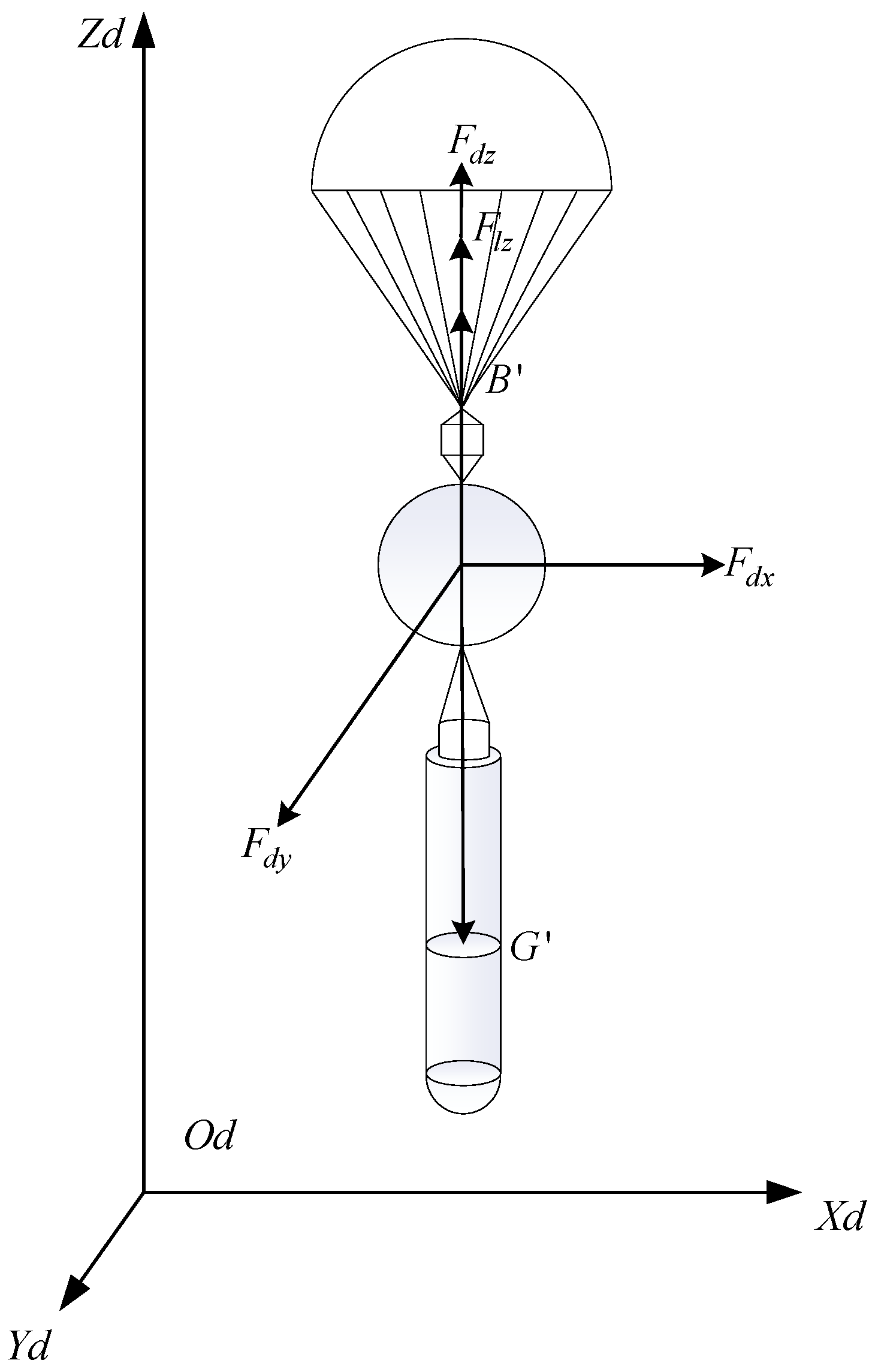
2.2. Dynamic Model of Parachute

The structures of parachutes vary depending on their different models, and their parameter descriptions also differ. In order to study the inflation process of parachutes, it is necessary to determine the system description parameters of the parachute under study [24].

The nominal diameter of the parachute is calculated as follows:

$$D_0=2\sqrt{A_0/\pi },$$

(6)

where $A_0$ is the nominal area. It is defined as the surface area of the whole canopy (including the area of the canopy top hole) after the parachute is expanded. $D_0$ is the nominal diameter.

The calculation formula of parachute projection area is as follows:

$$D_{\mathrm{p}}=2\sqrt{A_{\mathrm{p}}/\pi },$$

(7)

where $D_p$ is the parachute projection diameter. $A_p$ is the parachute projection area.

Figure 3 shows a diagram of the parachute force analysis, where h_p/R_p (the rise–radius ratio) is the ratio of the height to the radius of the parachute.

The parachute resistance is related to the speed of movement, air density, shape, and size. It can be expressed by the following formula:

$$D=C_{\mathrm{D}}{\displaystyle \frac{1}{2}}\rho v^{2}A,$$

(8)

where $C_{\mathrm{D}}$ represents the drag coefficient, indicating the level of air drag experienced by an object in motion. It depends on factors such as the shape of the object, its position in the airflow, and the Reynolds number [25]. A is the characteristic area. In this paper, the characteristic area is taken as the nominal area $A_0$.

In parachute calculations, a specific term called “drag characteristic” is used. The drag characteristic of a parachute is the product of its drag coefficient and the corresponding characteristic area, denoted as CD. It is defined as the product of the parachute resistance coefficient and the corresponding characteristic area.

$$CD=C_{\mathrm{D}}A$$

(9)

During a parachute drop test, the steady descent speed of the parachute and the air density at that time are measured. Based on the gravitational force acting on the suspended object, the effective drag coefficient of the parachute is calculated using the following formula:

$$C_{\mathrm{D}}={\displaystyle \frac{G_{\mathrm{s}}+G_{\mathrm{w}}}{\frac{1}{2}\rho {v_{\mathrm{d}}}^2{A}_0}},$$

(10)

where $G_{\mathrm{s}}$ is the gravitational weight of the mass of the parachute. $G_{\mathrm{w}}$ is the gravitational weight of the mass of the payload. $v_{\mathrm{d}}$ is the steady drop speed, which is measured in a wind tunnel.

The main aerodynamic force of the traditional symmetrical parachute is resistance, but it will also produce lift at a certain angle of attack. The component of the pressure difference between the upper and lower wing surfaces along the airflow coordinate axis ${oy}_q$ is the lift force L.

$$L=C_{\mathrm{L}}{\displaystyle \frac{1}{2}}\rho v^2{A}_0,$$

(11)

where $C_{\mathrm{L}}$ is the lift coefficient (relative to the nominal area $A_0$ of the canopy).

The additional mass is a parameter to calculate the fluid inertia of the external flow field during the parachute inflation process and the inertial influence of the stagnant airflow inside the canopy moving with the canopy, which has a very important influence on the dynamic characteristics of the parachute. The calculation method for the contained mass within the parachute canopy during the inflation process is as follows [26]:

$$m_{add}=m_i+m_a.$$

(12)

The additional mass is represented by the internal mass, which is equal to the air density multiplied by the volume inside the canopy, and the apparent mass. The mass contained in the parachute is calculated as follows:

$$m_i=\rho V,$$

(13)

where $V$ is the volume inside the parachute canopy, which varies with the inflation process.

Assuming that, during the inflation period, the shape of the parachute is an idealized form with a semi-spherical shape plus a truncated cone, the enclosed mass during the inflation process can be calculated using the following equation:

$$m_i={\displaystyle \frac{2\rho {D_0}^3}{3{\pi }^2}}\left[1.058-{\displaystyle \frac{{\left(T-1.31\right)}^2}{1.62}}\right],$$

(14)

where $T$ is a non-dimensional inflation time; $T=t/t_m$, $t_m$ is the time required to inflate the parachute, which is related to factors such as the parachute filling-time coefficient and atmospheric conditions, which can be determined experimentally; $D_0$ is the nominal diameter of the parachute canopy.

The formula for calculating the apparent mass is as follows:

$$m_a=\left(1+k\right)m_i,$$

(15)

where $k$ is a constant, which represents the ratio of the added mass to the inherent mass, which is typically related to the fluid dynamics, the shape of the parachute, and its motion state (such as acceleration, velocity, etc.).

After the deceleration parachute is deployed, it experiences predominantly horizontal forces from the wind field and vertical forces arising from the resistance, lift, and the payload’s gravity. The dynamic equations are as follows [27]:

$$\left\{\begin{array}{c}(m_{all}+m_{add})a_x=F_{dx}\\ (m_{all}+m_{add})a_y=F_{dy}\\ (m_{all}+m_{add})a_z=F_{dz}+F_{lz}+m_{all}g\end{array}\right.,$$

(16)

where $m_{all}$ is the total mass of the system; $a_x$, $a_y$, and $a_z$ are the acceleration in the directions of x, y, and z, respectively; $g$ is the local gravitational acceleration; $F_{dz}$, $F_{dx}$, and $F_{dy}$ are the air drag in the directions of x, y, and z, respectively; $F_{lz}$ is the vertical lifting force; and $m_{add}$ is the additional mass.

$$\left\{\begin{array}{c}{F}_{dx}={(C_{Dp})}_x{\displaystyle \frac{1}{2}}\rho {v_{rx}}^2{A}_x\\ F_{dy}={(C_{Dp})}_y{\displaystyle \frac{1}{2}}\rho {v_{ry}}^2{A}_y\\ F_{dz}={(C_{Dp})}_z{\displaystyle \frac{1}{2}}\rho {v_{rz}}^2{A}_z\end{array}\right.$$

(17)

$$F_{lz}=C_L{\displaystyle \frac{1}{2}}\rho {v_{rz}}^2{A}_z,$$

(18)

where $\rho$ is the local air density. ${({C_D}_p)}_x$, ${({C_D}_p)}_y$, and ${({C_D}_p)}_z$ are the drag coefficients of the parachute in three directions, indicating the degree of obstruction by the air when the object is in movement, which is related to the shape of the object, the position of the object in the airflow, the Reynolds number, etc. $C_L$ is the lift coefficient; $A_x$, $A_y$, and $A_z$ are the effective cross-sectional areas of the deceleration of the parachute; and $v_{rx}=v_x-v_{windx}$, $v_{ry}=v_y-v_{windy}$ and $v_{rz}=v_z$. $v_{windx}$ and $v_{windy}$ are wind speeds in the x and y directions, respectively.

The filling-time of the parachute is divided into three stages: (Stage 1) from starting to inflate to the first stage of the closing section; (Stage 2) maintaining the closing section; (Stage 3) lifting the closing section to the fully filled section [28]. The corresponding time is shown as follows:

$$\left\{\begin{array}{c}{t}_{m1}={\displaystyle \frac{\alpha K{D}_0}{{\nu }_l}} (\mathrm{Stage} 1)\\ t_{m2}=const(\mathrm{Preset} \mathrm{value}) (\mathrm{Stage} 2)\\ t_{m3}={\displaystyle \frac{K{D}_0}{{\nu }_l}} (\mathrm{Stage} 3)\end{array}\right.,$$

(19)

where $t_{m1}$ is the time of the first stage, $t_{m2}$ is the time of the second stage, $t_{m3}$ is the time of the third stage, $\alpha$ is the initial area ratio, $K$ is the filling-time coefficient of the parachute, which is related to the size, material, and structural design of the parachute, ${\nu }_l$ is the speed of the system at the beginning of inflation, and $D_0$ is the nominal diameter of the parachute. The resistance area of the canopy corresponding to the three stages of the canopy inflation process is

$$\left\{\begin{array}{c}(C_{p}S)={\displaystyle \frac{{(C_{p}S)}_{s1}}{t_{m1}}}t t_1\le t\le t_1+t_{m1} (\mathrm{Stage} 1)\\ \\ (C_{p}S)={(C_{p}S)}_{s1} t_1+t_{m1}\le t\le t_1+t_{m1}+t_{m2} (\mathrm{Stage} 2)\\ \\ (C_{p}S)={(C_{p}S)}_{s1}+[{(C_{p}S)}_{s2}-{(C_{p}S)}_{s1}]{({\displaystyle \frac{t-t_1}{t_2-t_1}})}^n t_1+t_{m1}+t_{m2}\le t\le t_2 (\mathrm{Stage} 3)\end{array}\right.,$$

(20)

where, $t_1$ and $t_2$ are the start and end times of the parachute inflation phase, respectively; $(C_{p}S)$ is the resistance area of the canopy, ${(C_{p}S)}_{s1}$ and ${(C_{p}S)}_{s2}$ are the resistance areas of the canopy at the end of the first stage of the inflation process and at the release of the second stage, respectively.

The change rate of the canopy resistance area corresponding to the three sections of the canopy inflation process is

$$\left\{\begin{array}{c}({\dot{C}}_{p}S)={\displaystyle \frac{{(C_{p}S)}_{s1}}{t_{m1}}} t_1\le t\le t_1+t_{m1} (\mathrm{Stage} 1)\\ \\ ({\dot{C}}_{p}S)=0 t_1+t_{m1}\le t\le t_1+t_{m1}+t_{m2} (\mathrm{Stage} 2)\\ \\ ({\dot{C}}_{p}S)=n[{\displaystyle \frac{{(C_{p}S)}_2-{(C_{p}S)}_{s1}}{t_2-t_1}}]{({\displaystyle \frac{t-t_1}{t_2-t_1}})}^{n-1} t_1+t_{m1}+t_{m2}\le t\le t_2 (\mathrm{Stage} 3)\end{array}\right..$$

(21)

The calculation method of the parachute opening dynamic load is as follows:

$$F_p=q(C_{p}S)+v_z{\displaystyle \frac{d{m}_a}{dt}}+(m_a+m_p){\displaystyle \frac{d{v}_z}{dt}}+m_{p}g\sin \theta ,$$

(22)

where $F_p$ is the opening dynamic load of the parachute, q is the dynamic pressure, $(C_{p}S)$ is the resistance area of the canopy, $v_z$ is the velocity in the vertical direction, $m_a$ is the additional mass, $m_j$ is the total mass of the system, and $\theta$ is the inclination angle.

2.3. Model of the Aerostat

Dynamics Model of the Aerostat

High-altitude balloons are usually filled with air and helium, which can float in the atmosphere [23]. The floating balloon contains an air bag and a helium bag. Assuming that both the helium and air within the balloon system satisfy the gas ideal equation of state, the relationship is as follows [29,30]:

$$\left\{\begin{array}{c}{P}_{he}{V}_{he}=m_{he}{R}_{he}{T}_{he}\\ P_{air}{V}_{air}=m_{air}{R}_{air}{T}_{air}\end{array}\right.,$$

(23)

where $P_{he}$ and $P_{air}$ are the pressures of helium and air, respectively; $V_{he}$ and $V_{air}$ are the volumes of helium and air, respectively; $m_{he}$ and $m_{air}$ are the masses of helium and air, respectively, $R_{he}$ and $R_{air}$ are the gas constants of helium and air, respectively; and $T_{he}$ and $T_{air}$ are the temperatures of helium and air, respectively. The total volume of the stratospheric aerostat is the sum of the volumes of the main helium envelope and the auxiliary air envelope. The main and auxiliary envelopes are interconnected by a diaphragm that transmits pressure. It can be assumed that the pressure in the main envelope is in equilibrium with the pressure in the auxiliary envelope, which is expressed as follows:

$$\left\{\begin{array}{c}V=V_{he}+V_{air}\\ P_{he}=P_{air}=P_{ref}+\Delta P\end{array}\right.,$$

(24)

where V is the total volume of the high-altitude balloon, P_ref is the outside atmospheric pressure, and $\Delta P$ is the pressure difference between the inside of the capsule and the outside atmospheric pressure.

During the flight of the stratospheric aerostat, the primary forces acting on it include buoyancy, gravity, additional inertia force, and aerodynamic forces. Due to the relatively minor influence of the altitude, the changes in the system altitude can be neglected. The stratospheric aerostat ascends in the vertical direction relying on net buoyancy, while it experiences drifting motion in the east–west direction along the horizontal plane carried by the wind. Throughout the flight process, it is subjected to forces such as gravity, buoyancy, aerodynamic forces, and additional inertia forces [31].

The buoyancy force on the aerostat is calculated by the following formula:

$$B={\rho }_{a}Vg,$$

(25)

where ${\rho }_a$ is the density of the air in the environment.

The gravitational force on the aerostat, which includes the helium, the balloon bladder, and the payload, is calculated by the following formula:

$$G=\left(m_{h\mathrm{e}}+m_{env}+m_{fu\_env}+m_{pay}\right)g,$$

(26)

where $m_{h\mathrm{e}}$ is the mass of helium gas, $m_{env}$ is the mass of the balloon bladder, $m_{fu\_env}$ is the additional mass of the balloon, and $m_{pay}$ is the mass of the payload.

The three components of aerodynamic forces in the ground coordinate system are

$$\left\{\begin{array}{c}{R}_x=-{\displaystyle \frac{1}{2}}{(C_{Da})}_x{\rho }_a{v}_x^{2}S\\ R_y=-{\displaystyle \frac{1}{2}}{(C_{Da})}_y{\rho }_a{v}_y^{2}S\\ R_z=-{\displaystyle \frac{1}{2}}{(C_{Da})}_z{\rho }_a{v}_z^{2}S\end{array},\right.$$

(27)

where $R_x$, $R_y$, and $R_z$ are the aerodynamic forces of the balloon in three directions; $v_x$, $v_y$, and $v_z$ are the three components of the balloon’s air-to-air velocity in ground coordinates, the air-to-air velocity can be obtained by adding the ground velocity to the wind speed, and the negative sign indicates that the balloon is subjected to aerodynamic force in the opposite direction of its motion. ${(C_{Da})}_x$, ${(C_{Da})}_y$, and ${(C_{Da})}_z$ are the drag coefficients of the aerostat in three directions, ${\rho }_a$ is the air density, and $S$ is the windward area of the balloon.

When an aerostat undergoes unsteady motion in the air, it induces the acceleration of the surrounding air, leading to an additional inertial force known as additional mass [32]. The magnitude of this force is proportional to the acceleration of the aerostat’s motion and is directed opposite to the acceleration. In this context, the aerostat is approximated as a spherical shape, and its additional mass can be directly derived from the velocity potential of the flow around it:

$${\lambda }_1={\lambda }_2={\lambda }_3={\displaystyle \frac{2}{3}}\pi R^3{\rho }_a,$$

(28)

where ${\lambda }_1$, ${\lambda }_2$, and ${\lambda }_3$ are the additional mass in the directions of x, y, and z, respectively; $R$ is the radius of aerostat’s balloon; and ${\rho }_a$ is the local air density.

In summary, as shown in Figure 4, the equations for the center-of-mass dynamics of the balloon in the ground coordinate system are obtained [33]:

$$\left\{\begin{array}{c}(m+{\lambda }_1)a_x=-{\lambda }_1{a}_x+R_x\\ (m+{\lambda }_2)a_y=B-{\lambda }_2{a}_y+R_y-G\\ (m+{\lambda }_3)a_z=-{\lambda }_3{a}_z+R_z\end{array}\right.,$$

(29)

where $a_x$, $a_y$, and $a_z$ are the acceleration components of the balloon relative to the ground coordinate system.

The equations of kinematics for the center of mass of the aerostat are as follows:

$$\left\{\begin{array}{c}{\displaystyle \frac{dx}{dt}}=v_x\\ {\displaystyle \frac{dy}{dt}}=v_y\\ {\displaystyle \frac{dz}{dt}}=v_z\end{array}\right..$$

(30)

2.4. Dynamics Model of the Deployment System

Figure 5 shows that there is a period that includes both the deceleration of the parachute and the inflation of the balloon during the rapid deployment process. At this stage, the parachute has fully deployed, and the balloon is inflating [34]. Therefore, the system in this state is referred to as the parachute–balloon system. The force analysis of the parachute–balloon system is shown in Figure 5.

The mass of the parachute can be calculated using the following equation:

$$\left\{\begin{array}{c}{m}_3=m_p+m_c\\ m_p=\sigma S_p\\ m_c=n{m}_{perc}\end{array}\right.,$$

(31)

where $\sigma$ is the aerial density of the parachute fabric. $S_p$ is the surface area of the parachute canopy. $n$ is the number of suspension lines. $m_{perc}$ is the mass of a single suspension line.

According to the potential flow theory, the calculation formula of the added mass $m_{bf}$ of the aerostat can be obtained. The Hess–Smith numerical method can be used to solve the velocity potential.

$$m_{bf}=C_{Bv}{m}_{bair},$$

(32)

where $C_{Bv}$ is the additional mass coefficient, and $m_{bair}$ is the air mass discharged by the aerostat. The balloon used herein is basically spherical, and its additional mass coefficient can be directly obtained from the velocity potential of the flow field around it: $C_{Bv}=0.5$.

The masses of various components of the rapid deployment aerostat system are as follows:

$$m_{system}=m_1+m_2+m_3+m_4+m_5,$$

(33)

where $m_{system}$ is the total mass of the system before parachute deployment. $m_1$ is the mass of the payload. $m_2$ is the mass of the inflation equipment. $m_3$ is the mass of the deceleration parachute system. $m_4$ is the mass of the balloon platform. $m_5$ is the mass of the cabin with other components.

$$G\prime =m_{system}g,$$

(34)

where $G\prime$ is the weight of the parachute–balloon system.

The balloon is inflated with helium, which is compressed in a gas cylinder. When the balloon needs to be inflated, helium is discharged from the gas cylinder into the balloon. The calculation method for the mass inflation rate is shown in the following formula:

$$e=c_1{A}_1\sqrt{{\displaystyle \frac{2\Delta p_1}{pg}}}$$

(35)

$${\displaystyle \frac{d{m}_{\mathrm{g}}}{dt}}=-{\rho }_{\mathrm{g}}e=-{\displaystyle \frac{p_{\mathrm{g}}{M}_{\mathrm{g}}}{R{T}_g}}e,$$

(36)

where e is the volume inflation rate, ${\rho }_g$ is the helium density under external pressure, $A_1$ is the exhaust area, $c_1$ is the discharge efficiency coefficient, $\Delta p_1$ is the pressure difference between the balloon and the high-pressure gas cylinder, and $p$ is the helium pressure.

The volume of the balloon changes over time, and its calculation method is as follows:

$$V\prime =et.$$

(37)

The buoyancy force on the aerostat is calculated by the following formula:

$$B\prime ={\rho }_{a}V\prime g.$$

(38)

The deceleration parachute experiences predominant horizontal forces from the wind field and vertical forces arising from the resistance, lift, and the whole system’s weight. The dynamic equations are as follows:

$$\left\{\begin{array}{c}(m_{system}+m_{add}+m_{bf})a_x=F_{dx}\\ (m_{system}+m_{add}+m_{bf})a_y=F_{dy}\\ (m_{system}+m_{add}+m_{bf})a_z=F_{dz}+F_{lz}+B\prime -G\prime \end{array}\right.,$$

(39)

where $m_{system}$ is the total mass of the system, $a_x$, $a_y$, and $a_z$ are the acceleration in the directions of x, y, and z, respectively; $g$ is the local gravitational acceleration, and $F_{dx}$, $F_{dy}$, and $F_{dz}$ are the air drag in the directions of x, y, and z, respectively; $F_{lz}$ is the vertical lifting force of the parachute, $m_{add}$ is the additional mass of the parachute, and $m_{bf}$ is the additional mass of the aerostat.

$$\left\{\begin{array}{c}{F}_{dx}={(C_{Ds})}_x{\displaystyle \frac{1}{2}}\rho {v_{rx}}^2(A_x+S_x)\\ F_{dy}={(C_{Ds})}_y{\displaystyle \frac{1}{2}}\rho {v_{ry}}^2(A_y+S_y)\\ F_{dz}={(C_{Ds})}_z{\displaystyle \frac{1}{2}}\rho {v_{rz}}^2\cdot max(A_z,S_y)\end{array}\right.$$

(40)

$$F_{lz}=C_L{\displaystyle \frac{1}{2}}\rho {v_{rz}}^2{A}_z,$$

(41)

where $\rho$ is the local air density. ${(C_{Ds})}_x$, ${(C_{Ds})}_y$, and ${(C_{Ds})}_z$ are the drag coefficients of the system, indicating the degree of obstruction by the air when the object is in movement, which is related to the shape of the object, the position of the object in the airflow the Reynolds number, etc. $C_L$ is the lift coefficient, $A_x$, $A_y$, and $A_z$ are the windward areas of the parachute in the x, y, and z directions, respectively, $S_x$, $S_y$, and $S_z$ are the windward areas of the balloon in the x, y, and z directions, respectively; $v_{rx}=v_x-v_{windx}$, $v_{ry}=v_y-v_{windy}$, and $v_{rz}=v_z$. $v_{windx}$ and $v_{windy}$ are the wind speeds in the x and y directions, respectively.

The equations of kinematics for the parachute–balloon system are as follows:

$$\left\{\begin{array}{c}{v}_x=v_{0x}+a_{x}t\\ v_y=v_{0y}+a_{y}t\\ v_z=v_{0z}+a_{z}t\end{array}\right.,$$

(42)

where $v_{0x}$, $v_{0y}$, and $v_{0z}$ are the initial velocities of the parachute–balloon system, respectively.

3. Results and Discussion

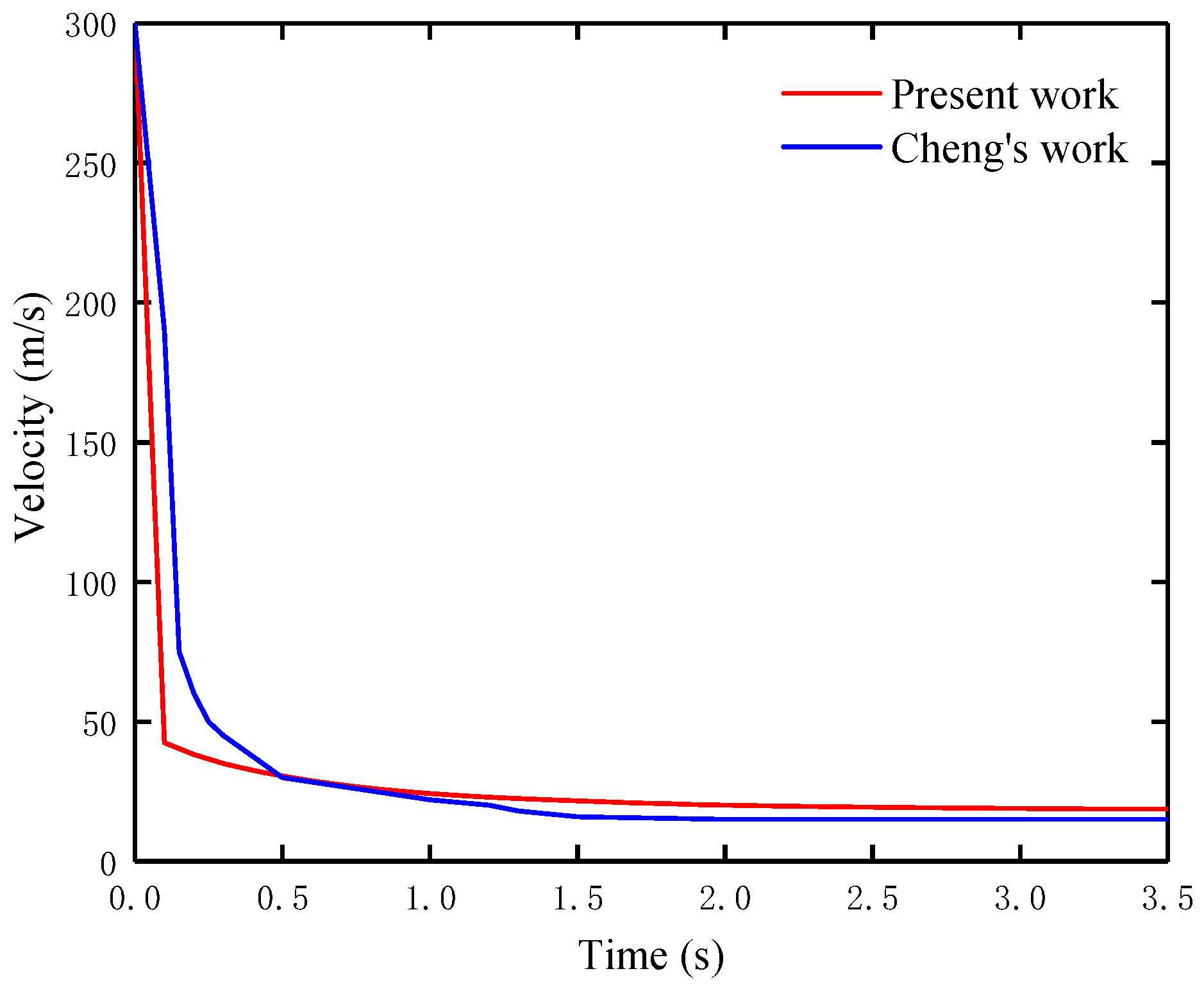
3.1. Model Verification

To verify the accuracy of the developed dynamics model of the parachute, the present work was compared with the results provided in the literature [22]. The input data selected from the literature included a drag coefficient (0.95) and an initial deployment velocity (300 m/s).

Figure 6 illustrates the comparison of the present work and Cheng’s work. After 0.5 s, the velocity in the present work closely aligned with Cheng’s work, and the difference remained within a small range. The deviation may be due to differences in the atmospheric models used, as varying air densities can affect the drag force. Overall, the trend between the present work and Cheng’s work was consistent, indicating that the parachute dynamics model is suitable for studying the parachute descent process. However, there is currently a lack of comprehensive experimental or flight test data to further verify the simulation results of the deployment process. This limitation confines the verification scope of the proposed model and will be addressed in future studies as more data become available.

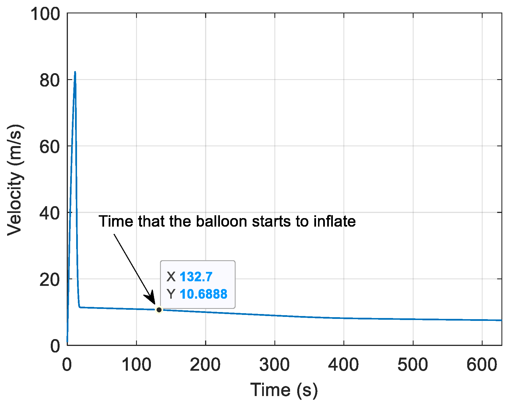
3.2. Simulation and Results

Simulations were conducted using MATLAB R2024b to explore how various parachute characteristics affected the performance of rapid-deployment aerostat systems. The inflation process in this study was simulated using LS-DYNA, in which the continuous decrease in pressure and flow rate during the process was considered. This simulation focused on the deployment process of a rapid-deployment aerostat system. The design parameters of the rapid-deployment aerostat system are detailed in

Table 1. Design parameters of the rapid-deployment aerostat system.

Parameters	Value	Parameters	Value
Atmospheric model	GB1920-80	Skin thermal emissivity	0.78
Wind field location	A central region in China	Parachute shape	Annular parachute
Deployment method	Air-based or missile-based	Surface density of parachute, g/m2	75
Velocity of system delivery, m/s	0	Velocity of parachute opening m/s	80
Release altitude, km	15	Percentage of the critical dynamic load	40%
Time of balloon inflation, s	300	Maximum dynamic load, N	10,000
Skin thickness, mm	0.7	Inflation gas	Helium
Skin areal density, g/m2	50	Types of gas cylinders	Composite high-pressure gas cylinder
Balloon skin density, kg/m3	2190	Gas cylinder pressure, Mpa	70
Balloon skin specific heat capacity, J/(kg·K)	1470	Inflation pressure, Mpa	2
Balloon skin thermal conductivity, W/(m·K)	0.29	Compressor inlet and outlet flow rate, L/s	150
Skin thermal absorptivity	0.21

. The maximum dynamic load must be below 40% of the critical dynamic load of 25,000 N, which is 10,000 N. Exceeding the limit load may lead to structural failure, aerodynamic asymmetry, severe oscillations, and control failure, thereby causing instability in the entire parachute system.

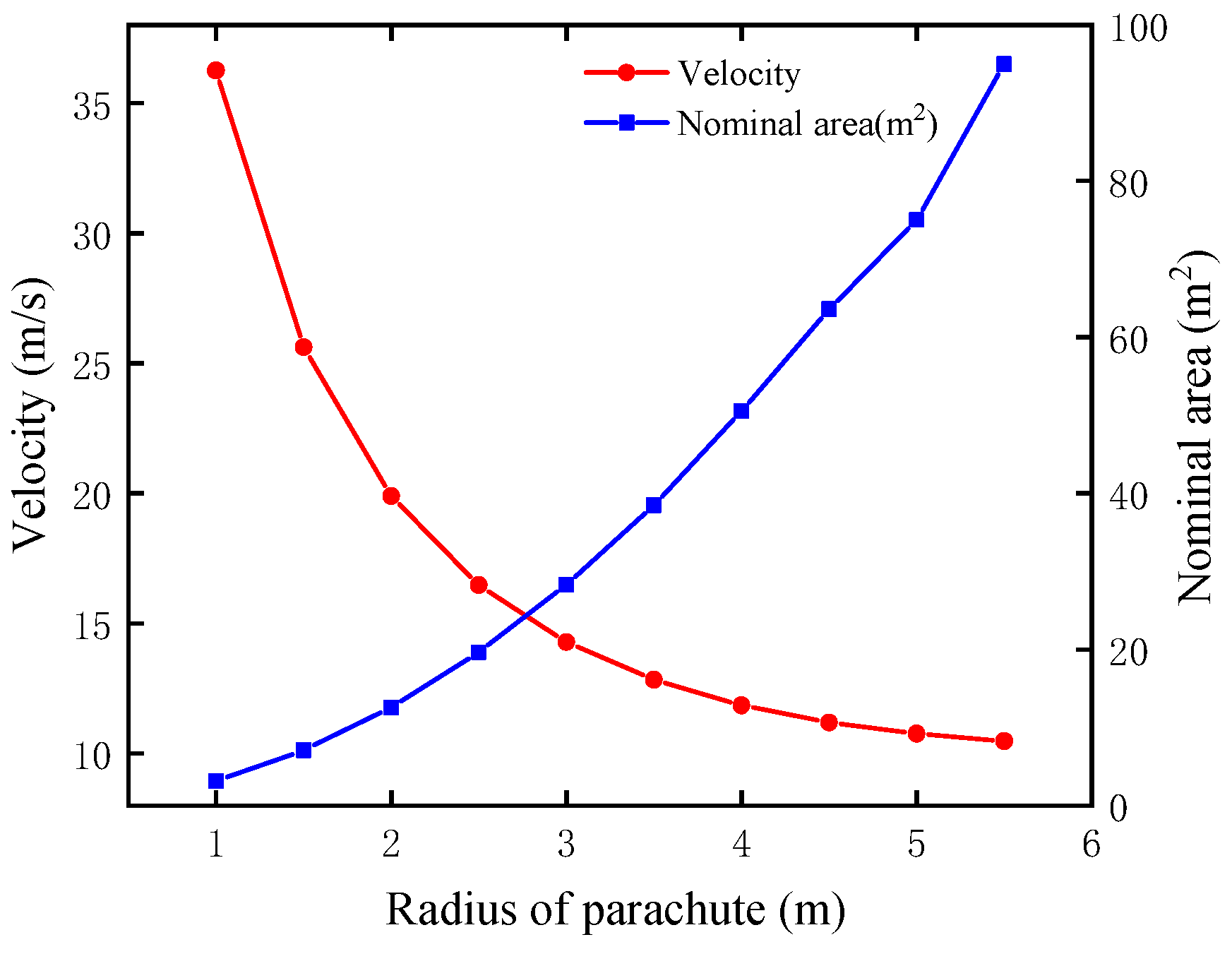
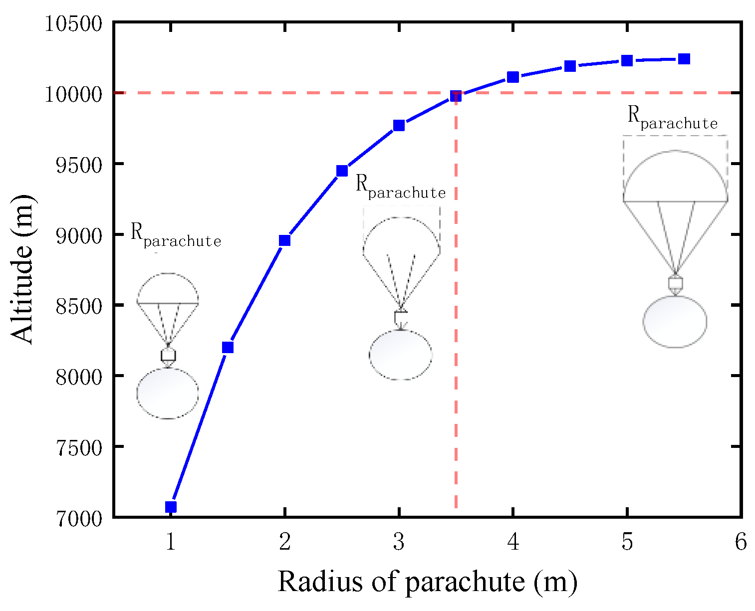
3.2.1. Analysis of the Nominal Radius of the Parachute

To better evaluate the deceleration performance, this study analyzes the descent velocity at the beginning of balloon inflation. Figure 7 shows the velocity variation over time for a parachute with a nominal radius of 5 m. Figure 8 illustrates the velocity when the balloon starts to inflate and the nominal area under different parachute nominal radii. It is clear that as the radius of the parachute increases, its nominal area also increases, resulting in an enhanced deceleration effect. When the nominal radius increases from 1 m to 2 m, the velocity when the balloon begins to inflate drops from 36 m/s to 20 m/s. However, when the nominal radius exceeds 2 m to 5.5 m, the velocity when the balloon inflates deceases smoothly from 20 m/s to about 10 m/s. This indicates that the unit deceleration effect achieved by increasing the parachute’s unit nominal area diminishes. Additionally, the parachute’s nominal area increases from 3 m² to 96 m² as the nominal radius of the parachute increases from 1 m to 5.5 m, leading to more material and higher cost requirements.

To ensure that the balloon completes inflation at a sufficiently high altitude and avoids conflicts with civil and military airspace, this study analyzes the system’s altitude at the end of the inflation process. An example is shown in Figure 9, illustrating the altitude variation with time when the nominal radius of the parachute is 5 m. Figure 10 shows the altitude when the balloon’s inflation is completed. The altitude when the balloon’s inflation is completed declines with the increase in the nominal radius of the parachute. At the beginning, when the radius increases from 1 m to 4.5 m, the altitude rises from about 7000 m to 10,200 m. However, with the increase in the parachute’s nominal radius from 4.5 m to 5.5 m, the height remains stable at 10,200 m. For parachutes with a nominal radius of less than 3.5 m, the balloon cannot finish inflating above 10,000 m. Here, 10,000 m was chosen to avoid conflicts with most civil and military aircraft.

The maximum dynamic load experienced by the deceleration parachute during the descent process directly affects the structural safety of the canopy material, suspension lines, and connection components. Therefore, this study analyzes the maximum dynamic load on the parachute throughout the entire deployment process. As shown in Figure 11, the dynamic load variation is presented for the case where the nominal radius of the parachute is 5 m. Figure 12 illustrates the maximum dynamic load of a parachute during deployment for different nominal radii of the parachute. The maximum dynamic load increases with the increase in the nominal radii of the parachute. The maximum dynamic load rises from approximately 2500 N to about 15,000 N when the nominal radius increases from 1 m to 5.5 m. When the parachute’s nominal radius is less than or equal to 4.25 m, the maximum dynamic load remains below 10,000 N. However, when the parachute’s nominal radius exceeds 4.25 m, the maximum dynamic load exceeds 10,000 N, which may lead to parachute instability.

The maximum dynamic pressure reflects the most severe aerodynamic loading on the parachute. Excessive dynamic pressure may lead to canopy deformation or structural failure, especially during high-speed descent or early inflation stages. In this study, the dynamic pressure experienced by the system is analyzed over the entire deployment process. Figure 13 illustrates the variation in dynamic pressure when the nominal radius of the parachute is 5 m. Figure 14 depicts the maximum dynamic pressure under different nominal radii of a parachute. The maximum dynamic pressure decreases with the increase in the nominal radii of a parachute. At the beginning, the maximum dynamic load drops sharply from almost 200 Pa to 80 Pa with the increase in the parachute’s nominal radius from 1 m to 2 m. After that, the dynamic pressure begins to decline gradually from approximately 80 Pa to about 50 Pa with the increase in the radius from 2 m to 4 m. At the end, the dynamic pressure remains stable at almost 50 Pa.

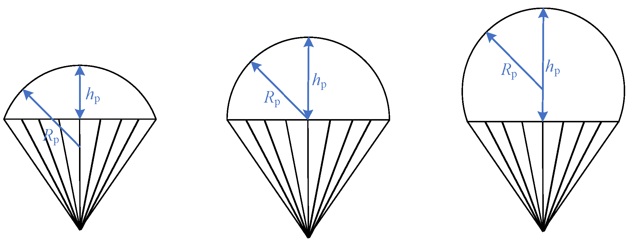
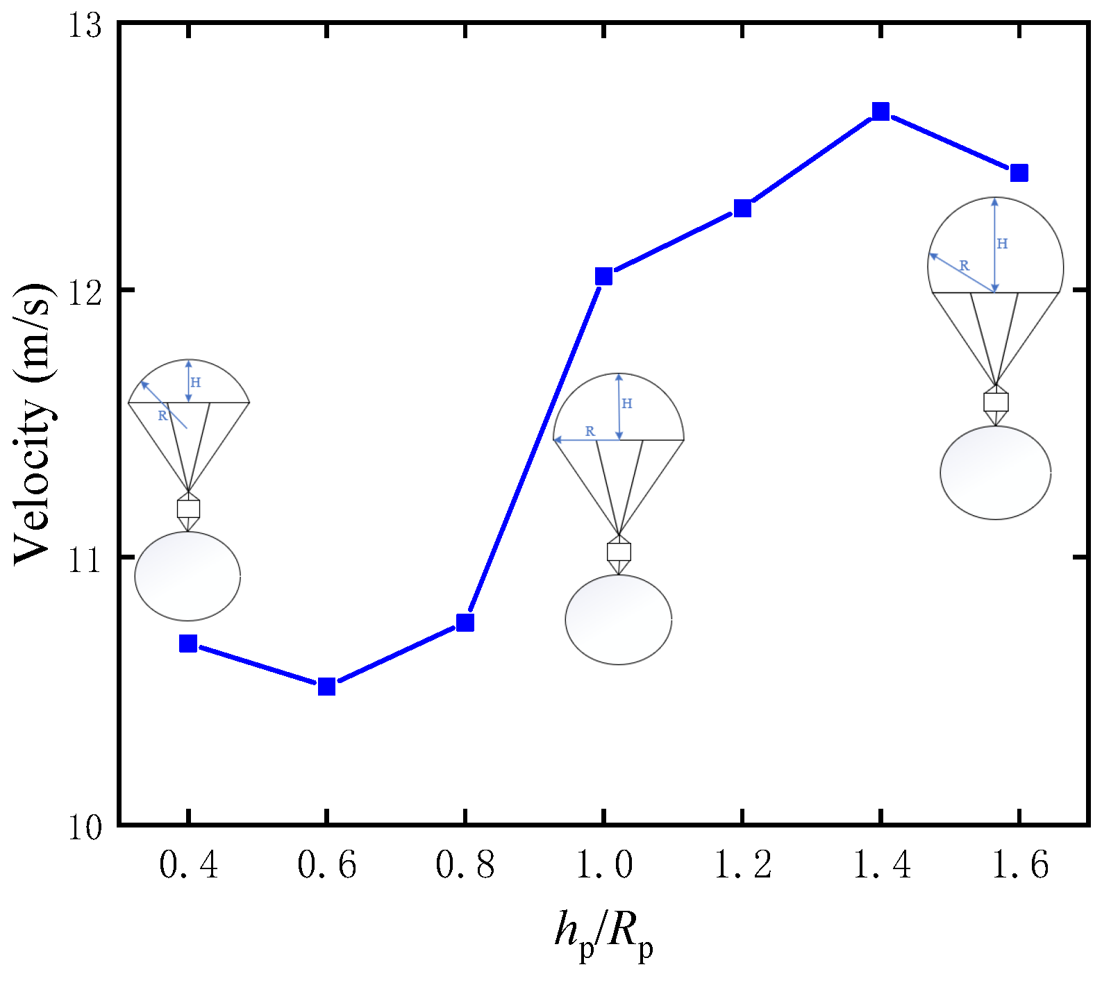
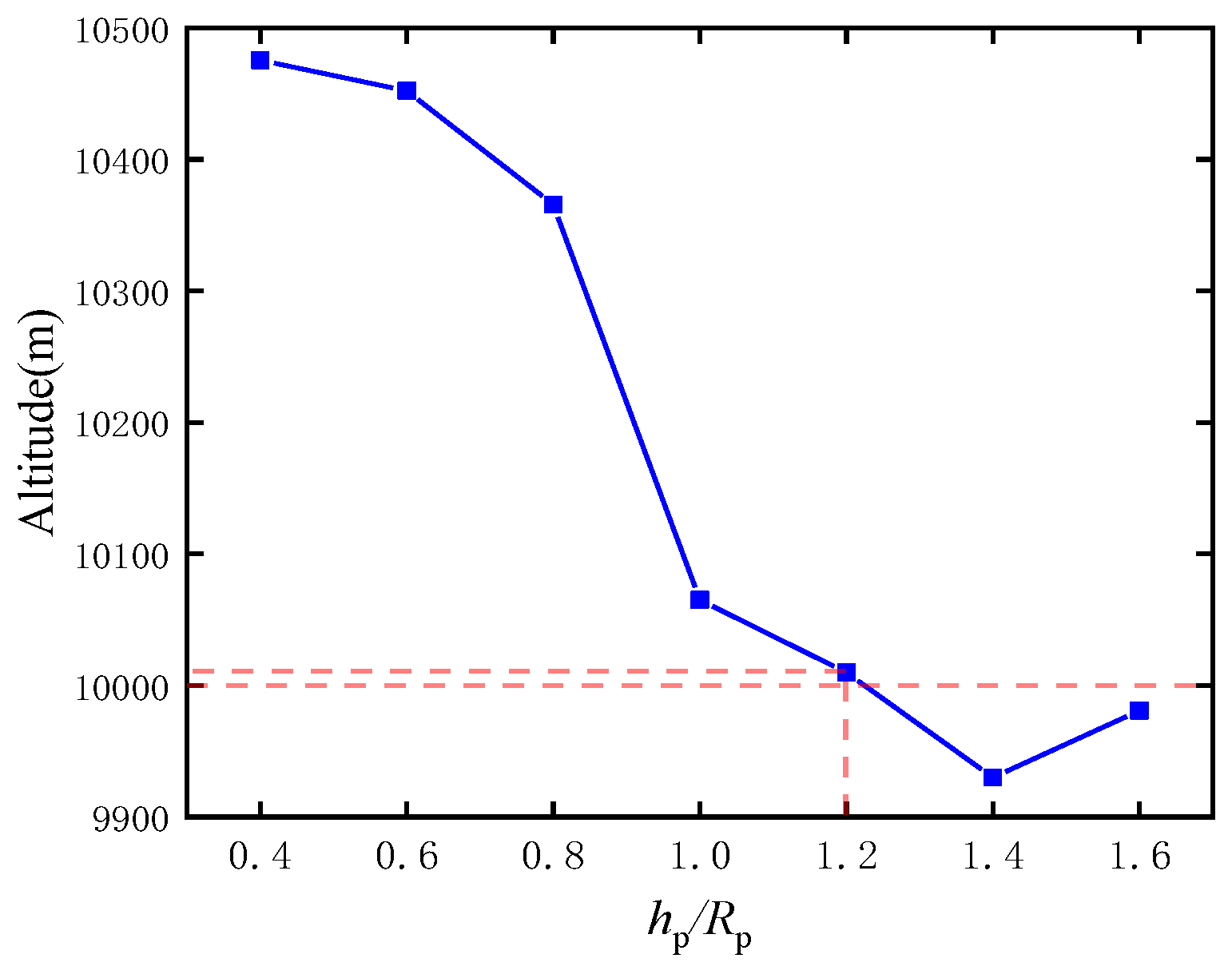
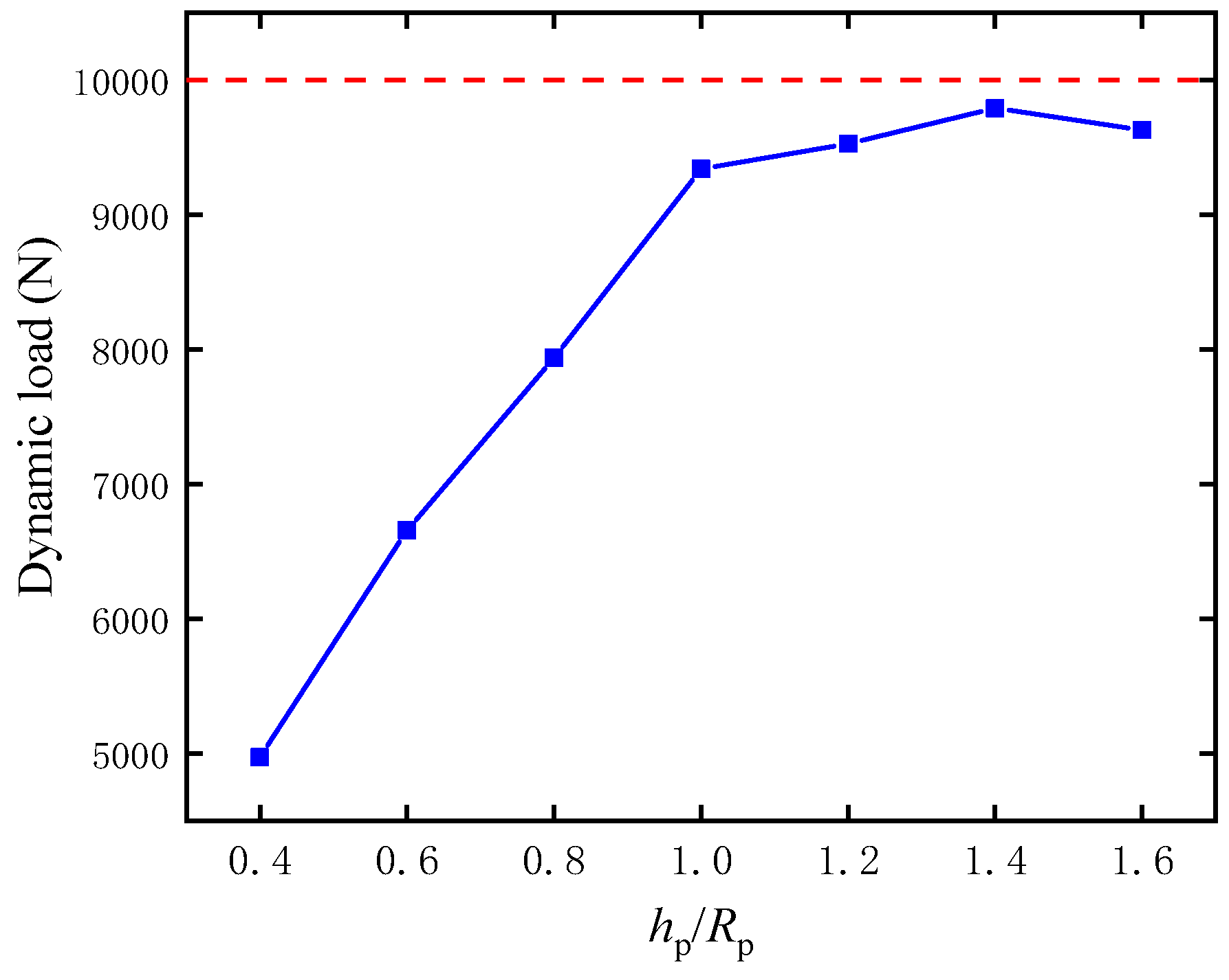
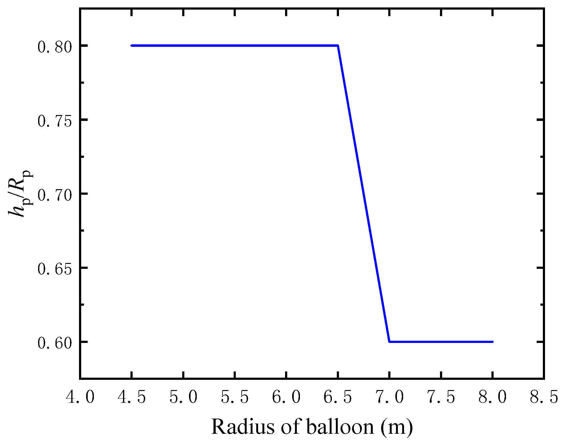
3.2.2. Analysis of the Rise–Radius Ratio of the Parachute

Figure 15 shows parachutes with different h_p/R_p values. In order to study the influence of the h_p/R_p of the parachute on the rapid deployment process, this study used computational fluid dynamics (CFD) to analyze the aerodynamic drag of parachutes with different h_p/R_p values.

The wind pressure distribution on the parachute surface is described using the wind pressure coefficient, defined as the ratio of the wind pressure on the parachute surface to the dynamic pressure corresponding to the parachute’s descent speed. It is stipulated that when the wind pressure is directed away from the surface along the surface normal, the coefficient is negative, and when directed toward the surface, it is positive. The drag coefficient is the ratio of the integral of the wind pressure coefficient over the surface area vector to the parachute’s projected area. The drag coefficient (CD) can be determined using the ratio of the pressure difference between the inside and outside of the parachute to the dynamic pressure corresponding to the descent velocity of the parachute. The drag characteristic is obtained by multiplying the drag coefficient by the nominal area of the parachute.

A contour plot of the wind pressure coefficient distribution on the inner and outer surfaces of the h_p/R_p =1 parachute is given in Figure 16. The set descent speed of the parachute is 10 m/s, and the calculated dynamic pressure is 64.5 Pa. Through fluent simulations, the internal pressure is 70.49 Pa, with an average wind pressure coefficient on the internal surface of 1.09. The external pressure is −17.38 Pa, with an average wind pressure coefficient on the external surface of 0.27. The drag coefficient is determined to be 1.36 after calculating the ratio of the pressure difference between the internal and external pressures to the dynamic pressure.

Figure 17 depicts the change in the drag coefficient (CD) and drag characteristic (C_D) with an increase in h_p/R_p. It can be seen that both CD and C_D decrease with the increase in h_p/R_p. Initially, CD declines sharply from almost 2.3 to 1.25 when h_p/R_p increases from 0.4 to 1.4. However, CD begins to increase gradually by approximately 0.1 when h_p/R_p increases from 1.4 to 1.6, possibly because of the fully spherical parachute being more prone to turbulence during descent, which increases the drag.

C_D increases sharply from approximately 70 m² to about 85 m² when h_p/R_p increases from 0.2 to 0.6, which causes a large increase in drag. C_D remains stable at 85 m² before C_D reaches the maximum at about 86 m² when h_p/R_p reaches 0.8. C_D drops from 86 m² to almost 62 m² when h_p/R_p increases from 0.8 to 1.4. However, when h_p/R_p increases from 1.4 to 1.6, C_D increases slightly from 62 m² to approximately 64 m² as a result of the increase in CD. C_D at h_p/R_p = 0.6 is a slightly lower drag coefficient compared to h_p/R_p = 0.8 but uses less fabric.

Figure 18 shows the velocity when the balloon starts to inflate under different h_p/R_p values. When the balloon starts to inflate, the velocity increases with the increase in h_p/R_p. At the beginning, with the increase in h_p/R_p from 0.4 to 0.6, the velocity decreases slightly from almost 10.7 m/s to 10.5 m/s and reaches the lowest point at 10.5 m/s. However, the velocity increases from 10.5 m/s to 12.7 m/s when h_p/R_p increases from 0.6 to 1.4, which is attributed to the drag coefficient decreasing with the increase in h_p/R_p. When h_p/R_p increases from 1.4 to 1.6, the velocity decreases from 12.7 m/s to 12.5 m/s again. This reduction is due to the drag characteristic becoming larger, increasing the overall drag and enhancing the deceleration effectiveness.

Figure 19 illustrates the altitude when balloon inflation is complete under different h_p/R_p values of the parachute. The altitude when balloon inflation is complete decreases with the increase in h_p/R_p. When h_p/R_p increases from 0.4 to 1.4, the altitude decreases from approximately 10,500 m to 9900 m. After that, the altitude increases from approximately 9900 m to 10,000 m when h_p/R_p increases from 1.4 to 1.6. The altitude drops below 10,000 m when h_p/R_p = 1.4, although the curve begins to rise slightly when h_p/R_p > 1.4, but it still remains below 10,000 m.

Figure 20 illustrates the maximum dynamic load of the parachute under different h_p/R_p values of a parachute. It is evident that the maximum dynamic load decreases with the increase in h_p/R_p. When h_p/R_p increases from 0.4 to 1.4, the maximum dynamic load increases from 5000 N to almost 9800 N. After that, the influence of h_p/R_p on the maximum dynamic load is significant, but it consistently remains below 10,000 N. When h_p/R_p is 1.6, the dynamic load decreases to about 9700 N, which may be attributed to the consistent projected area. The maximum dynamic load remains below 10,000 N, signifying excellent stability.

Figure 21 illustrates the maximum dynamic pressure for different h_p/R_p values. The maximum dynamic pressure decreases from about 50.5 Pa to 50 Pa with the increase in h_p/R_p from 0.4 to 0.6, the maximum dynamic pressure increases from about 50 Pa to 60 Pa with the increase in h_p/R_p from 0.6 to 1.4, and it reaches its highest point (60 Pa) when h_p/R_p is 1.4. However, the maximum dynamic pressure declines from 60 Pa to almost 59 Pa when h_p/R_p decreases from 1.4 to 1.6.

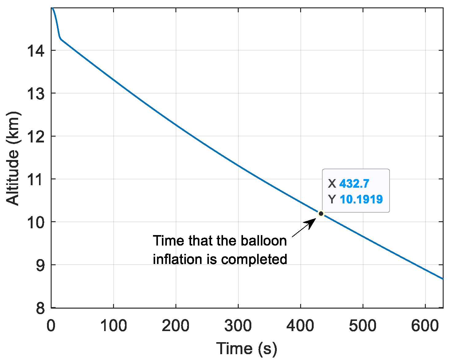
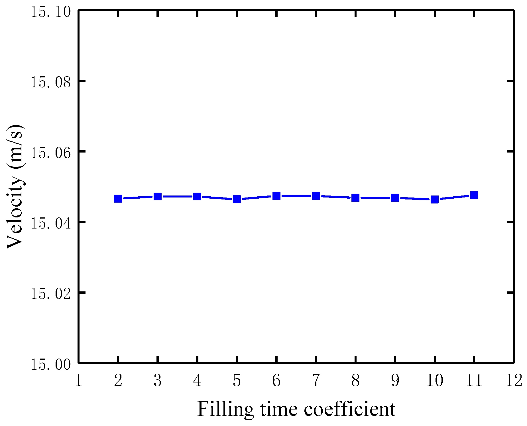
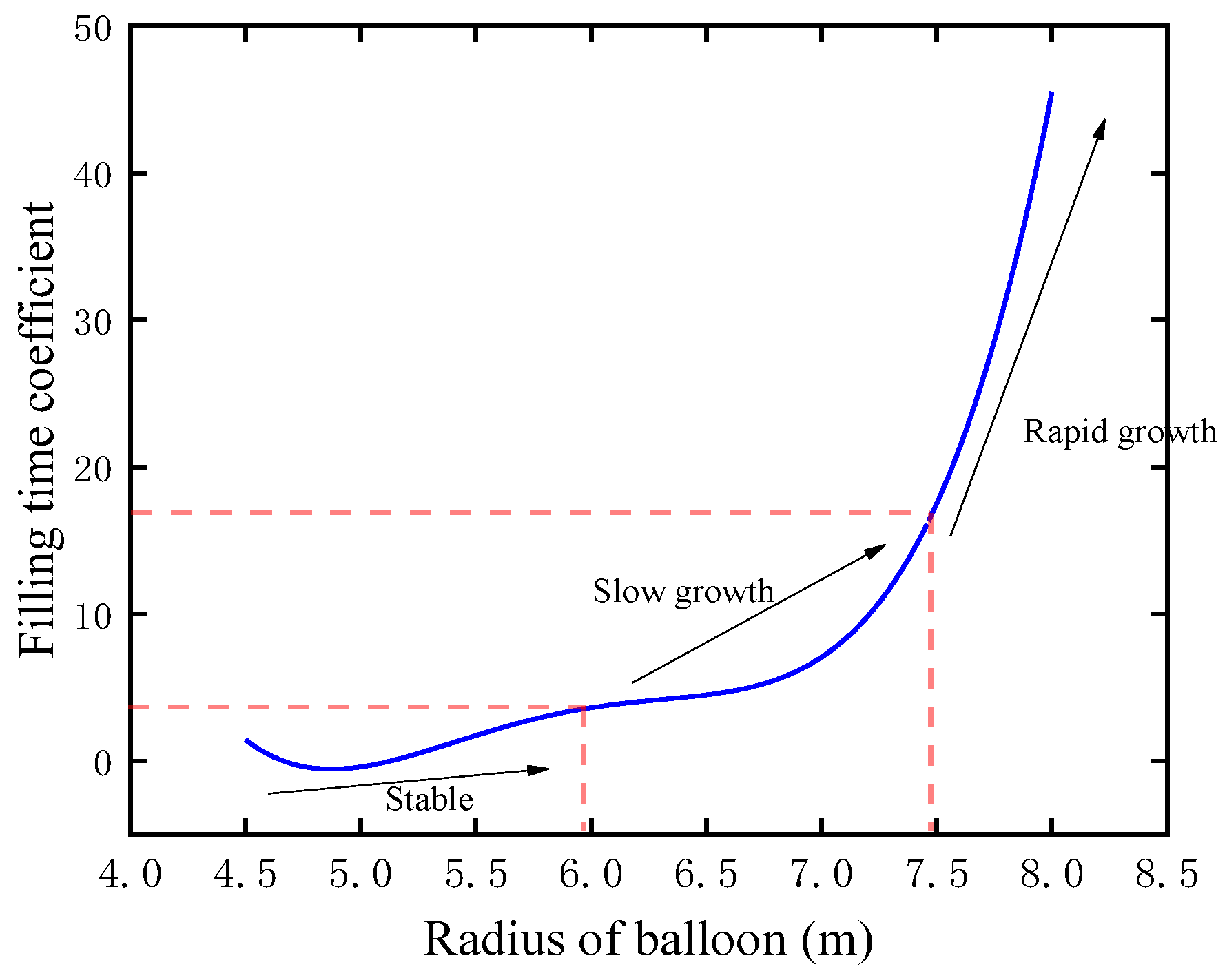
3.2.3. Analysis of the Filling-Time Coefficient of the Parachute

Figure 22 shows the velocity when the balloon starts to inflate under different filling-time coefficients of the parachute. It can be seen that the velocity remains stable with the change in the filling-time coefficient: as the filling-time coefficient increases from 2 to 11, the velocity remains unchanged at almost 15.05 m/s. This indicates that the filling-time coefficient has little effect on the velocity when the balloon starts to inflate.

Figure 23 illustrates the altitude when the balloon’s inflation is completed under different filling-time coefficients. It is clear that the altitude fluctuates with the change in the filling-time coefficient of the parachute, but the variation is minimal. The altitude fluctuates around 10,038.5 m with the change in the filling-time coefficient from 2 to 11. This suggests that changes in the filling-time coefficient have a minimal impact on the altitude, with a difference within 1 m. Regardless of the chosen filling-time coefficient, the system completes deployment at altitudes above 10,000 m.

Figure 24 illustrates the maximum dynamic load experienced during the deployment process under different filling-time coefficients. The maximum dynamic load declines smoothly when the filling-time coefficient increases. The maximum dynamic load drops from approximately 12,800 N to about 9000 N when the filling-time coefficient increases from 2 to 11. When the filling-time coefficient is less than or equal to 4, the maximum dynamic load exceeds 10,000 N, which may lead to parachute instability. Maintaining a filling-time coefficient above 5 ensures that the maximum dynamic load stays below 10,000 N.

Figure 25 shows the maximum dynamic pressure under different filling-time coefficients. It is evident that the maximum dynamic load fluctuates with the change in the filling-time coefficient of the parachute, but the variation is minimal. The maximum dynamic pressure decreases slightly from about 57.27 Pa to 57.28 Pa with the increase in the filling-time coefficient from 2 to 5. The maximum dynamic pressure is maintained at about 57.27 Pa when the filling-time coefficient increases from 2 to 9. After that, the maximum dynamic pressure increases slightly from about 57.26 Pa to 57.28 Pa with the increase in the filling-time coefficient from 9 to 11. The dynamic pressure is not strongly affected by the filling-time coefficient. This is because the peak dynamic pressure generally occurs immediately before parachute deployment, when the velocity reaches its maximum; therefore, the filling-time coefficient has a negligible influence on the dynamic pressure.

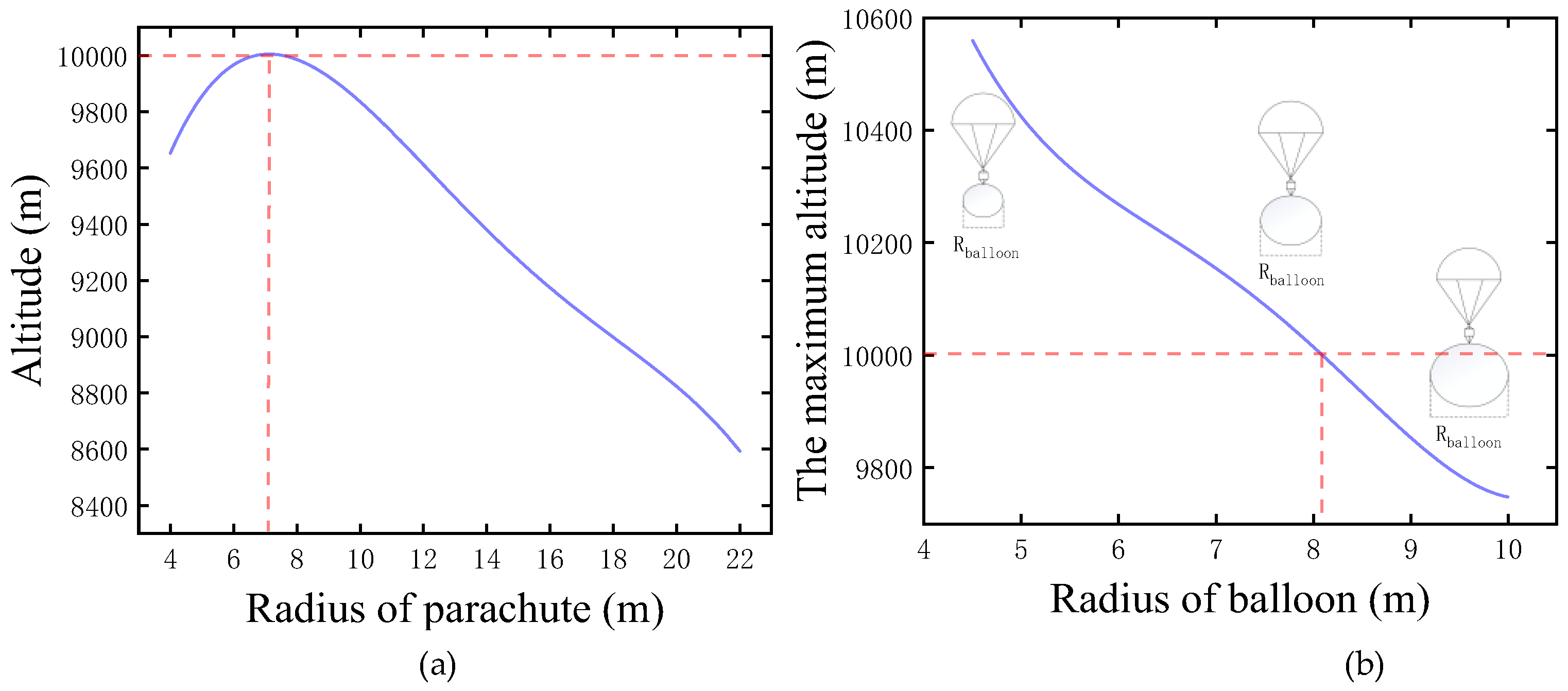
3.2.4. Design of the Parachute for Different Aerostats

In application, various loads may lead to changes in the radii of the balloon. It is necessary to consider different balloon radii to determine the corresponding optimal parachute radius, h_p/R_p, and the filling-time coefficient, based on the criteria of achieving the highest possible final inflation altitude, minimizing the dynamic pressure, reducing the parachute fabric area as much as possible, and keeping the filling-time coefficient as low as possible.

The optimal parachute nominal radius and area corresponding to the radii of the balloon are illustrated in Figure 26. It is clear that the optimal parachute nominal radius and area increase with the increase in the radii of the balloon. As the radii of the balloon increases from 4.5 m to 8.0 m, the optimal parachute radius gradually increases from almost 1.8 m to 6.4 m. There is a slow growth when the radius of the balloon increases from 4.5 m to 7.0 m before a rapid growth with the radius of the balloon increasing from 7.0 m to 8.0 m. The nominal area of the parachute increases from 10 m² to 128 m² as the radius of balloon increases from 4.5 m to 8.0 m, and the increase becomes more and more rapid. This suggests that the larger the radius of the balloon, the larger the radius of the parachute required. Additionally, the effectiveness of increasing the parachute’s unit nominal area diminishes due to the increased weight of the fabric associated with the larger nominal areas.

It can be seen in Figure 27a that the altitude as the balloon’s inflation is completed initially increases and then decreases with the increase in the radius. Firstly, when the radius of the balloon is 8 m, the altitude when the balloon’s inflation is completed increases with the increase in the parachute nominal radius from 4 m to 7 m and reaches the top at 10,000 m, which is the maximum altitude when the balloon’s inflation is completed, which can be reached by adjusting the radius of the parachute. However, when the parachute’s nominal radius increases from 7 m to 22 m, the altitude starts to decrease to almost 8600 m. This is because larger parachute nominal areas require heavier fabrics, resulting in increased system weight. Figure 27b depicts the maximum altitude that can be reached when the balloon’s inflation is completed by adjusting the radius of the parachute under different radii of the balloon. It is clear that the maximum altitude decreases with the increase in the radius of the balloon, and the height is under 10,000 m when the radius of balloon is greater than 8 m, which means that, when the radius of balloon is greater than 8 m, regardless of the chosen nominal radius of the parachute, the altitude remains below 10,000 m. Hence, when the radius of balloon exceeds 8 m, it is recommended not to use a rapid-deployment aerostat system.

Figure 28 shows the relationship between the radius of the parachute and the minimum acceptable parachute filling-time coefficient. It is obvious that the minimum acceptable parachute filling-time coefficient increases when the radius of the parachute increases. When the radius of the parachute increases from 4.5 m to 6 m, the acceptable minimum filling-time coefficient stays unchanged at 2 or 3. After that, when the radius of the parachute increases from 6 m to 7.5 m, the acceptable minimum filling-time coefficient increases from 3 to about 17 and jumps to 46 when the radius of the parachute increases from 7.5 m to 8 m. As the radius of the parachute increases, the mass of the total cabin increases too, and a greater filling-time coefficient is required to ensure the stability and safety of the system. For a larger radius of a balloon, the rapid increase in the filling-time coefficient may be due to the larger parachute area to decelerate; thus, it takes a longer time to fully deploy the parachute.

Figure 29 shows the optimal parachute h_p/R_p corresponding to different radii of the balloon. When the radius of the balloon increases from 4.5 m to 6.5 m, the optimal h_p/R_p remains unchanged at 0.8. However, when the radius of the balloon increases from 6.5 m to 7.0 m, the optimal h_p/R_p drops to 0.6. This reduction in h_p/R_p for a larger radii of the balloon is due to the need to reduce the maximum dynamic loads, ensuring system stability. After that, the optimal h_p/R_p remains unchanged again at 0.6 when the mass of the cabin increases from 7.0 m to 8.0 m. Therefore, a parachute with h_p/R_p = 0.8 for the radius of a balloon below 6.5 m and an h_p/R_p = 0.6 for the radius of a balloon over 6.5 m is recommended.

4. Conclusions

In this study, combining the dynamics models of parachutes and stratospheric aerostats, a program was developed to thoroughly investigate the impact of the radius, rise–radius ratio, and filling-time coefficient of a parachute on the deployment process of rapid-deployment aerostat systems. In addition, the optimal parachute nominal radius, rise–radius ratio, and filling-time coefficient were analyzed for different radii of a balloon.

The main conclusions can be summarized as follows:

• Increasing the radius enhances the deceleration effectiveness but raises the maximum dynamic loads and the cost of the parachute. When the nominal radius increases from 1 m to 5.5 m, the velocity when the balloon begins to inflate deceases from 36 m/s to about 10 m/s.
• The rise–radius ratio significantly affects the drag characteristic of the parachute, which means that it significantly affects the deceleration performance of the parachute. The drag characteristic reaches its maximum at about 86 m² when h_p/R_p is 0.8.
• The increase in the filling-time coefficient will lead to a significant reduction in the dynamic load of the parachute. The maximum dynamic load drops from approximately 12,800 N to 9000 N when the filling-time coefficient increases from 2 to 11.
• The system cannot be deployed above 10 km by changing the parachute radius when the balloon radius exceeds 8 m. A larger filling-time coefficient is required as the radius of balloon increases. A parachute with h_p/R_p = 0.8 for the radius of a balloon below 6.5 m and an h_p/R_p = 0.6 for the radius of a balloon over 6.5 m is recommended.

The influence of parachute characteristics on the rapid-deployment aerostat system was investigated in this study. The obtained results are helpful for guiding the rapid-deployment aerostat system. Additionally, the influence of the wake, meteorological conditions, material properties, and other factors on the stability and performance of the rapid-deployment aerostat system can be considered in the next stage of work. Moreover, future research is encouraged to conduct targeted experiments or develop benchmark datasets to support more extensive validation of the proposed simulation models.

References

1. Li, J.; Ling, L.; Liao, J.; Chen, Z.; Luo, S. Effect of Lifting Gas Diffusion on the Station-Keeping Performance of a Near-Space Aerostat. Aerospace 2022, 9, 328. [Google Scholar] [CrossRef]
2. Anoop, S.; Velamati, R.K.; Oruganti, V.R.M. Aerodynamic characteristics of an aerostat under unsteady wind gust conditions. Aerosp. Sci. Technol. 2021, 113, 106684. [Google Scholar] [CrossRef]
3. Zuo, Z.; Song, J.; Zheng, Z.; Han, Q.-L. A survey on modelling, control and challenges of stratospheric airships. Control Eng. Pract. 2022, 119, 104979. [Google Scholar] [CrossRef]
4. Riboldi, C.E.; Rolando, A. Thrust-based stabilization and guidance for airships without thrust-vectoring. Aerospace 2023, 10, 344. [Google Scholar] [CrossRef]
5. Zhang, L.; Li, J.; Jiang, Y.; Du, H.; Zhu, W.; Lv, M. Stratospheric airship endurance strategy analysis based on energy optimization. Aerosp. Sci. Technol. 2020, 100, 105794. [Google Scholar] [CrossRef]
6. Shan, C.; Sun, K.; Ji, X.; Cheng, D. A reconfiguration method for photovoltaic array of stratospheric airship based on multilevel optimization algorithm. Appl. Energy 2023, 352, 121881. [Google Scholar] [CrossRef]
7. Jiang, Y.; Lv, M.; Chen, X.; Wu, Y. An optimization approach for improving the solar array output power of stratospheric aerostat. Aerosp. Sci. Technol. 2021, 118, 106916. [Google Scholar] [CrossRef]
8. Jiang, Y.; Lv, M.; Sun, K. Effects of installation angle on the energy performance for photovoltaic cells during airship cruise flight. Energy 2022, 258, 124982. [Google Scholar] [CrossRef]
9. Xie, M.; Long, Y.; Deng, X.; Yang, X. Station-keeping of Stratospheric Aerostat with Receding Horizon Tree Search Planning Method. J. Phys. Conf. Ser. 2022, 2410, 012008. [Google Scholar] [CrossRef]
10. Zhang, Y.; Zhu, M.; Chen, T.; Zheng, Z. Distributed event-triggered fixed-time formation and trajectory tracking control for multiple stratospheric airships. ISA Trans. 2022, 130, 63–78. [Google Scholar] [CrossRef]
11. Yang, X.; Yang, X.; Deng, X. Horizontal trajectory control of stratospheric airships in wind field using Q-learning algorithm. Aerosp. Sci. Technol. 2020, 106, 106100. [Google Scholar] [CrossRef]
12. Yuan, J.; Guo, X.; Zheng, Z.; Zhu, M.; Gou, H. Error-constrained fixed-time trajectory tracking control for a stratospheric airship with disturbances. Aerosp. Sci. Technol. 2021, 118, 107055. [Google Scholar] [CrossRef]
13. Shi, Z.; Huo, W.; Zuo, Z. Motion-pressure coupled control and simulation of long-endurance capability for multicapsule stratospheric airships. Chin. J. Aeronaut. 2024, 37, 137–150. [Google Scholar] [CrossRef]
14. Zhou, R.; Li, J.; Yang, Z.; Xu, Y.; Yu, Z.; Zhang, Y. Fractional-Order Sliding-Mode Fault-Tolerant Control of Unmanned Airship Against Actuator Faults. IFAC-PapersOnLine 2022, 55, 617–622. [Google Scholar] [CrossRef]
15. Jiang, Y.; Lv, M.; Wang, C.; Meng, X.; Ouyang, S.; Wang, G. Layout optimization of stratospheric balloon solar array based on energy production. Energy 2021, 229, 120636. [Google Scholar] [CrossRef]
16. Sun, P.; Long, F.; Cheng, H. Experimental and numerical study on rapid inflation process of air-launched balloon. Ind. Textila 2022, 73, 268–274. [Google Scholar] [CrossRef]
17. Babu, K.K.; Pant, R.S. A review of Lighter-than-Air systems for exploring the atmosphere of Venus. Prog. Aerosp. Sci. 2020, 112, 100587. [Google Scholar] [CrossRef]
18. Bai, Y.; Kang, R.; Gao, Y.; Fu, W. The design of aerostat platform system’s parameters which is launched form a ballistic missile. In Proceedings of the 2018 IEEE CSAA Guidance, Navigation and Control Conference (CGNCC), Xiamen, China, 10–12 August 2018. [Google Scholar]
19. Gatto, V.L.; Izraelevitz, J.S.; Pauken, M.T.; Goel, A.; Lam, R.; Hall, J.L. Inflation sequence tradeoffs and laboratory demonstration of a prototype variable-altitude venus aerobot. Acta Astronaut. 2024, 214, 757–773. [Google Scholar] [CrossRef]
20. El-Sadi, H.; Kruzyk, E.; Ashik, K.; Alcantara, C. Study the Effect of the Diameter of Annular Parachute on Drag Using CFD. Available online: https://avestia.com/MCM2023_Proceedings/files/paper/HTFF/HTFF_148.pdf (accessed on 3 July 2024).
21. Tripathy, S. Aerodynamics of Parachutes of Different Configurations and Sizes. 2023. Available online: https://papers.ssrn.com/sol3/papers.cfm?abstract_id=4499469 (accessed on 9 November 2024).
22. Cheng, H.; Ouyang, Y.; Zhang, Y.; Pan, J. Research on the influence of length-width ratio on cruciform parachute airdropping performance. J. Ind. Text. 2022, 51 (Suppl. 5), 7694S–7713S. [Google Scholar] [CrossRef]
23. López, D.; Domínguez, D.; Delgado, A.; García-Gutiérrez, A.; Gonzalo, J. Experimental Calculation of Added Masses for the Accurate Construction of Airship Flight Models. Aerospace 2024, 11, 872. [Google Scholar] [CrossRef]
24. Pepermans, L.; Britting, T.; Jodehl, J.; Menting, E.; Sujahudeen, M. Architectures for parachute testing. J. Space Saf. Eng. 2023, 10, 35–44. [Google Scholar] [CrossRef]
25. Hou, X.-Y.; Hu, J.; Yu, Y. Numerical study on ring slot parachute finite mass inflation process and wake recontact phenomenon. Aerosp. Sci. Technol. 2022, 128, 107763. [Google Scholar] [CrossRef]
26. Nie, S.; Yu, L.; Sun, Z.; Wu, Z. Analytical model for the air permeability of parachute fabric and structure parameters sensitivity analysis. J. Text. Inst. 2022, 113, 761–768. [Google Scholar] [CrossRef]
27. Cao, Y.; Wei, N. Flight trajectory simulation and aerodynamic parameter identification of large-scale parachute. Int. J. Aerosp. Eng. 2020, 2020, 5603169. [Google Scholar] [CrossRef]
28. Zhang, S.Y.; Yu, L.; Masarati, P.; Qiu, B.W. New general correlations for opening shock factor of ram-air parachute airdrop system. Aerosp. Sci. Technol. 2022, 129, 107844. [Google Scholar] [CrossRef]
29. An, W.; Lin, T.; Wang, S. Optimal structural design for a certain near-space composite propeller of airship using adaptive region division blending model. Chin. J. Aeronaut. 2023, 37, 301–316. [Google Scholar] [CrossRef]
30. Sun, L.; Sun, K.; Guo, X.; Yuan, J.; Zhu, M. Prescribed-time error-constrained moving path following control for a stratospheric airship with disturbances. Acta Astronaut. 2023, 212, 307–315. [Google Scholar] [CrossRef]
31. Zhu, Q.; Tang, X.; Tong, M. Study on unsaturated shapes of helium ballonet of rigid airship during ascent process. Aerosp. Sci. Technol. 2021, 118, 107001. [Google Scholar] [CrossRef]
32. Manikandan, M.; Pant, R.S. Research and advancements in hybrid airships—A review. Prog. Aerosp. Sci. 2021, 127, 100741. [Google Scholar]
33. Wachlin, J.; Ward, M.; Pacheco, J.; Costello, M. Design and testing of an ultra-low-power persistent parachute use logger. Aerosp. Sci. Technol. 2023, 132, 108017. [Google Scholar] [CrossRef]
34. Yang, X.; Zhang, W.; Hou, Z. Improved thermal and vertical trajectory model for performance prediction of stratospheric balloons. J. Aerosp. Eng. 2015, 28, 04014075. [Google Scholar] [CrossRef]
Figure 1. The rapid-deployment aerostat system.
Aerospace 12 00481 g001
Figure 2. Rapid-deployment process.
Aerospace 12 00481 g002
Figure 3. Diagram of the parachute force analysis.
Aerospace 12 00481 g003
Figure 4. Diagram of aerostat force analysis.
Aerospace 12 00481 g004
Figure 5. Diagram of the parachute–balloon system force analysis.
Aerospace 12 00481 g005
Figure 6. Comparison of the present work and Cheng’s work.
Aerospace 12 00481 g006
Figure 7. Velocity variation with time when the nominal radius of the parachute is 5 m.
Aerospace 12 00481 g007
Figure 8. The velocity when the balloon begins to inflate and the nominal area under different nominal radii of the parachute.
Aerospace 12 00481 g008
Figure 9. Altitude variation with time when the nominal radius of the parachute is 5 m.
Aerospace 12 00481 g009
Figure 10. The altitude when the balloon’s inflation is completed under different nominal radii of the parachute.
Aerospace 12 00481 g010
Figure 11. The dynamic load when the nominal radius of the parachute is 5 m.
Aerospace 12 00481 g011
Figure 12. The maximum dynamic load under different nominal radii of a parachute.
Aerospace 12 00481 g012
Figure 13. The dynamic pressure when the nominal radius of the parachute is 5 m.
Aerospace 12 00481 g013
Figure 14. The maximum dynamic pressure under different nominal radii of the parachute.
Aerospace 12 00481 g014
Figure 15. Parachutes with different rise–radius ratios.
Aerospace 12 00481 g015
Figure 16. The inner and outer surface wind pressures of a parachute when hp/Rp = 1.
Aerospace 12 00481 g016
Figure 17. Drag coefficient and drag characteristic corresponding to different hp/Rp of a parachute.
Aerospace 12 00481 g017
Figure 18. The velocity when the balloon begins to inflate under different hp/Rp of a parachute.
Aerospace 12 00481 g018
Figure 19. The altitude when the balloon’s inflation is completed under different hp/Rp values of a parachute.
Aerospace 12 00481 g019
Figure 20. The maximum dynamic load under different hp/Rp values of a parachute.
Aerospace 12 00481 g020
Figure 21. The maximum dynamic pressure under different hp/Rp of a parachute.
Aerospace 12 00481 g021
Figure 22. The velocity when the balloon begins to inflate under different filling-time coefficients of the parachute.
Aerospace 12 00481 g022
Figure 23. The altitude when the balloon’s inflation is completed under different filling-time coefficients of the parachute.
Aerospace 12 00481 g023
Figure 24. The maximum dynamic load under different filling-time coefficients of the parachute.
Aerospace 12 00481 g024
Figure 25. The maximum dynamic pressure under different filling-time coefficients of a parachute.
Aerospace 12 00481 g025
Figure 26. The optimal parachute radius and area corresponding to different radii of the balloon.
Aerospace 12 00481 g026
Figure 27. Analysis of the parachute’s radius for different radii of the balloon: (a) the altitude when the balloon’s inflation is completed; (b) the maximum altitude when the balloon’s inflation is completed.
Aerospace 12 00481 g027
Figure 28. The minimum acceptable parachute filling-time coefficient under different radii of a balloon.
Aerospace 12 00481 g028
Figure 29. The optimal parachute hp/Rp corresponding to different radii of a balloon.
Aerospace 12 00481 g029