Article

Symbolic Regression-Based Modeling for Aerodynamic Ground-to-Flight Deviation Laws of Aerospace Vehicles

1
State Key Laboratory of Aerodynamics, China Aerodynamics Research and Development Centre, Mianyang 621000, China
2
Computational Aerodynamics Institute, China Aerodynamics Research and Development Centre, Mianyang 621000, China
3
Facility Design and Instrumentation Institute, China Aerodynamics Research and Development Centre, Mianyang 621000, China
*
Author to whom correspondence should be addressed.
Aerospace 2025, 12(6), 455; https://doi.org/10.3390/aerospace12060455
Submission received: 26 March 2025 / Revised: 20 April 2025 / Accepted: 22 April 2025 / Published: 22 May 2025
(This article belongs to the Special Issue Flight Dynamics, Control & Simulation (2nd Edition))

Abstract

:
The correlation between aerodynamic data obtained from ground and flight tests is crucial in developing aerospace vehicles. This paper proposes methods for modelling this correlation that combine feature extraction and symbolic regression. The neighborhood component analysis (NCA) method is utilized to extract features from the high-dimensional state space and then symbolic regression (SR) is applied to find the concise optimal expression. First, a simulation example of the NASA Twin Otter aircraft is used to validate the NCA and the SR tool developed by the research team in modeling the aerodynamic coefficient deviation between ground and flight due to an unpredictable inflight icing failure. Then, the method and tool are applied to real flight tests of two types of aerospace vehicles with different configurations. The final optimized mathematical models show that the two vehicles’ pitching moment coefficient deviations are related to the angle of attack (AOA) only. The mathematical model built using NCA and the SR tool demonstrates higher fitting accuracy and better generalization performance for flight test data than other typical data-driven methods. The mathematical model delivers a multi-fold enhancement in fitting accuracy over data-driven methods for all fight cases. For UAV flight test data, the average root mean square error (RMSE) of the mathematical model demonstrates a maximum improvement of 37% in accuracy compared to three data-driven methods. For XRLV flight test data, the prediction accuracy of the mathematical model shows an enhancement exceeding 80% relative to Gaussian kernel SVM and Gaussian process data-driven models. The research verifies the feasibility and effectiveness of the data feature extraction combined with the symbolic regression method in mining the correlation law between ground and flight deviations of aerodynamic characteristics. This study provides valuable insight for modeling problems with finite data samples and explicit physical meanings.

1. Introduction

The wind tunnel test is crucial for studying the aerodynamic characteristics of aerospace vehicles. However, the real gas effect, scale effect, wall interference, and flow similarity in ground tests can lead to significant discrepancies between the aerodynamic ground test data and the actual flight data. Analyzing the deviations between aerodynamic data from ground tests, including wind tunnel and computational fluid dynamics (CFD) data and the actual flight data, is known as a correlation study. The objective of the correlation study is to create a more precise aerodynamic database model for vehicle development to better predict aerodynamic characteristics during actual flight.
The correction or extrapolation of wind tunnel test data was one of the popular research branches of aerodynamic ground-to-flight correlation analysis [1,2,3]. Recently, considerable research efforts have been devoted to problems with strongly nonlinear properties in ground effects and transonic and hypersonic flow regimes, such as using neural networks to estimate aerodynamic characteristics under the ground effect [4], hypersonic vehicle stage separation [5,6], boundary layer transition [7,8] and CFD-based ground test data corrections for transonic business jet aircraft [9,10]. The main goal of ground-to-flight correlation analysis is to establish a ground aerodynamic database that can better approximate the real flight. To date, the processing methods for the ground-to-flight aerodynamic deviations can be categorized as follows:
  • Proportional correction method. This method uniformly adjusts ground data deviations using a proportional coefficient. It is an easy-to-implement modeling method but lacks a mathematical–physical basis and generalization capability.
  • Key factor correction method. This method only focuses on one effect of the key factors, as in a real gas effect correction study [11].
  • Incremental modeling method. This method models the ground-to-flight deviation as an increment of the aerodynamic basic model. The aerodynamic extrapolation equation is then determined by identifying the increment from the flight data as a black box using machine learning [12,13,14,15] or parameter identification methods [16,17,18,19]. This black box approach does not consider the physical or mathematical meanings of the increment. To overcome the shortcomings of black box modeling, a physical law mining-based method has been proposed in recent years. This method aims to obtain correlation formulas with precise physical meanings. It has better generalization and extensibility performance than the black box model. One example is the multidimensional spatial-correlation-theory-based parse-matrix evolution algorithm proposed by Luo et al., which was used to explore hypersonic flow laws and similar parameters [20,21].
These correction methods cannot model the overall biases between ground and real flight and are mostly used in wind tunnel test data correction. In contrast, the black box deviation modeling methods lack generalization and interpretability and require large-scale data size in modeling. The physical law mining-based method appears to address the shortcomings of both correction and black box modeling methods, and it has therefore emerged as a promising direction for studying aerodynamic ground-to-flight deviations.
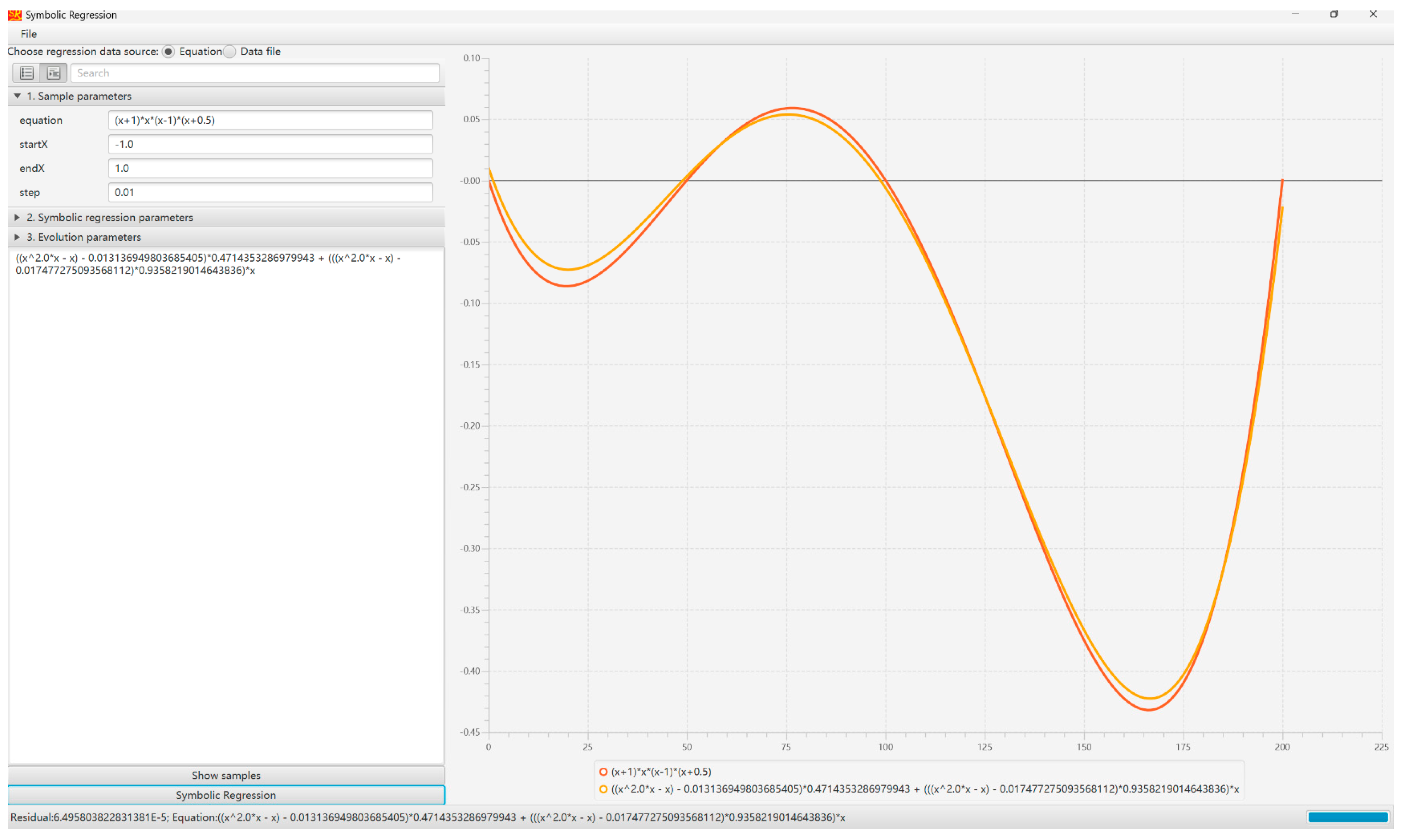
The symbolic regression method can be utilized in physical law mining, which has gained significant attention since the 1990s [22,23] and has been widely applied in various fields, such as chemical systems [24], fluid dynamics [25], dynamical systems [26,27,28,29] and natural science modeling [30]. The early application of the genetic-based evolutionary symbolic regression algorithm was limited to the difficulty of realizing the tree-structured formula expression in universal programming languages (UPLs). Consequently, several improvements have been made to the structure of the formula. For instance, attempts have been made to use binary coding to replace the tree structure [31] and a parse matrix-based encoding and decoding method to map from a two-dimensional matrix to function expression [20]. França [32] proposed a greedy search tree heuristic algorithm to exclude a region of rugged search space and complicated expressions. Cozad and Sahinidis [33] put forward a deterministic optimization algorithm, namely a mixed-integer nonlinear programming (MINLP) approach, to avoid the stochastic nature of genetic algorithms in symbolic regression and verified the method’s performance in eliminating formula redundancies and symmetries. Additionally, Petersen et al. [34] introduced reinforcement learning in symbolic regression to realize the best search direction autoregression. In the comparison between symbolic regression and neural networks, it was found that symbolic regression methods based on evolutionary algorithms could obtain a mathematical–physical model with stronger interpretability [35]. However, the issues of fitting accuracy and efficiency for high-dimensional space have remained a focus of research in symbolic regression.
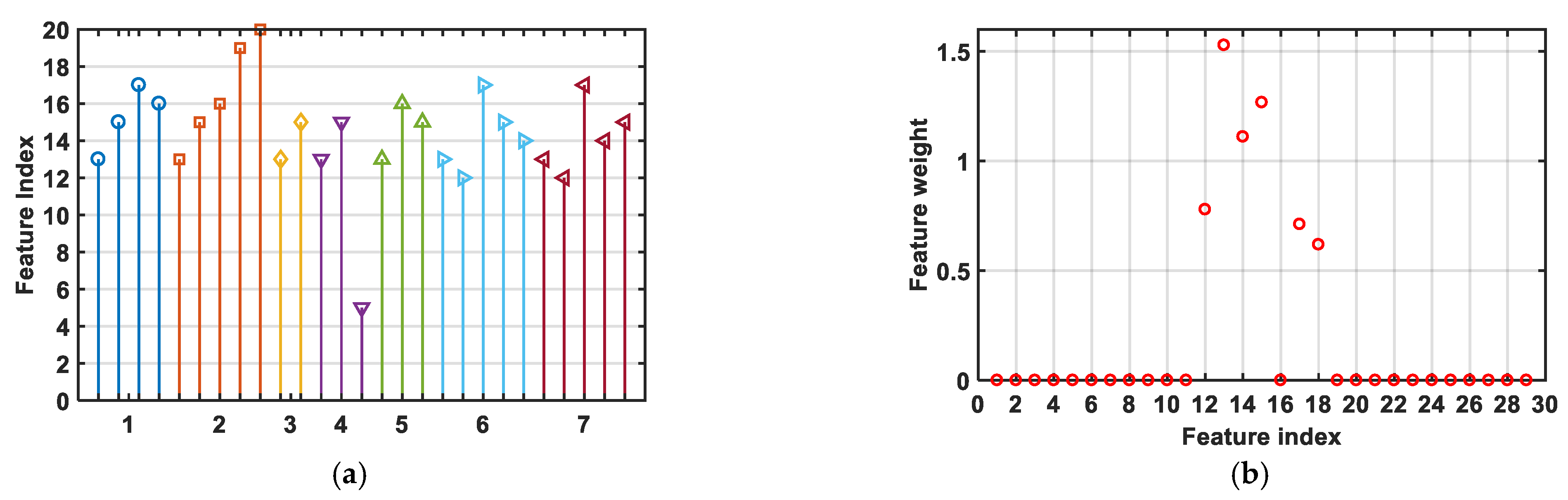
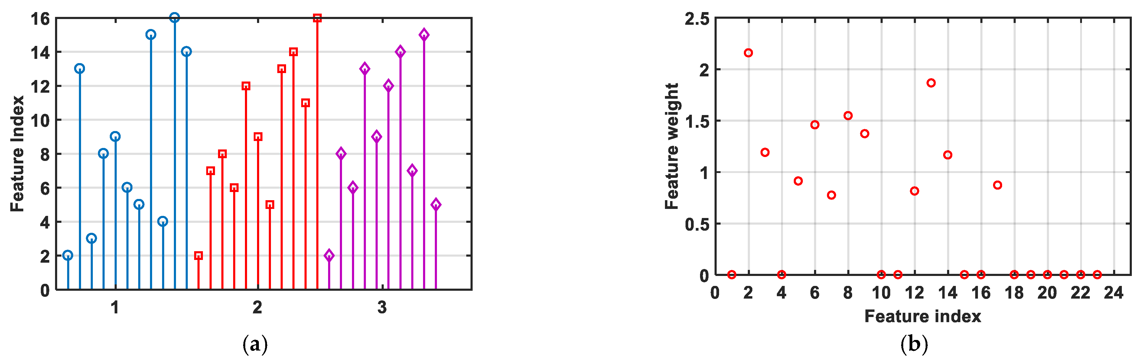
Current studies on the ground-to-flight correlation of aircraft aerodynamic characteristics mainly focus on wind tunnel test data corrections and theoretical analysis, while data-driven modeling mostly adopts black box models. This paper proposes conducting research on physical mechanism exploration and mathematical modeling of ground-to-flight deviations in aircraft aerodynamic characteristics of aerospace vehicles, aiming to establish an interpretable mathematical model with explicit physical significance. Such research remains relatively scarce in current academic investigations. The symbolic regression method is applicable for modeling the correlation between the aerodynamic ground test data and flight test data, but the challenge of efficiently extracting concise and physically interpretable mathematical expressions from high-dimensional flight state spaces remains to be addressed. To address this issue, a dimensional reduction technique is applied in this paper to enhance the efficiency of symbolic regression. The study faces another challenge in ground-to-flight correlation research: the unavailability of obtaining extensive flight test data due to the costs. Therefore, based on assumptions of flow similarity and the intrinsic physical connections between flight tests and ground tests for the same vehicle, this study combines correlation feature extraction with symbolic regression to address the challenges of physical law modeling from the aerodynamic ground-to-flight deviations in high-dimensional state space and with finite flight test data. The universality and effectiveness of this methodology is validated by two distinct types of aerospace vehicles. The findings demonstrate that the method can rapidly and efficiently identify physical laws governing the ground-to-flight deviation across the entire state space of different aerospace vehicles.
The paper is organized as follows: first, Section 2 introduces the symbolic regression tool and feature extraction method. Next, the two methods are validated using simulation data and applied on real flight deviations in the Section 3. Finally, the paper concludes with the Section 4.

2. Correlation-Feature-Extraction-Based Symbolic Regression

2.1. Symbolic Regression Tool

Given a data set Ɗ = (xi, yi), i = 1, 2, ⋯, n, where xi∈ℝd is a d-dimensional input vector and yi∈ℝ is a scalar output. Let be a function set consisting of mappings f: ℝd →ℝ. Define a sum of squares loss function for every candidate f. The optimization task is to find the function f over the set of that minimizes the loss.
L f = i = 1 n y i f x i 2 f = arg min f F L f
In symbolic regression, a library of elementary arithmetic operators and mathematical functions defines the set of , and the candidate functions are random combinations or mutations of the elements in this library.
Symbolic expressions are conventionally expressed in a sequential form using either a tree structure or other encoding methods. Genetic programming (GP) is an evolutionary algorithm for the optimization problem Equation (1). The initial generation is created randomly. Afterwards, the algorithm cycles through the following loops of mutation, crossover, evaluation, and selection until it reaches convergence or stopping criteria.
The project team developed a GP-based symbolic regression tool using tree structure expression (GPSR) (see Figure 1). The tool encapsulates the Jenetics toolkit in Java 21 and uses the Matlab 2017b toolkit to simplify the regressed functions. Subsequent research in this paper will utilize this GPSR toolkit.

2.2. Feature Extraction Method

The variables that have an essential impact on the regression parameter y are extracted from the state space by correlation analysis of the input and output to achieve state-space dimensionality reduction. Neighborhood component analysis (NCA) [36] is one of the most popular pattern classification techniques. The method belongs to the category of metric learning and directly maximizes the stochastic variant of the leave-one-out classification accuracy on the training set. Yang and Laaksonen [37] focused on the generalization and overfitting of NCA in high-dimensional spaces and proposed a regularized NCA algorithm. Classification, clustering and dimensionality reduction were typical application scenarios of NCA [38,39,40].
The regularized NCA algorithm is briefly reviewed for the following applications. Given a labeled data set Ɗ = (xi, yi), i = 1, 2, ⋯, n. Similarly, n denotes the sample size, xi is a d-dimensional vector and yi is the corresponding class label or regression scalar. Let A∈ℝr×d denote the transformation matrix, where r is the output dimension of input space and rd; then, the distance metric [36,39] can be expressed as
D x i x j = A x i A x j T A x i A x j , i , j = 1 , 2 , , n
The NCA algorithm computes the expected leave-one-out error from a stochastic variant of K-nearest neighbors (KNN) classification. The probability pij of each point xi selecting another point xj as its neighbor is calculated by a softmax over Euclidean distance in the transformed space:
p i j = exp A x i A x j 2 k i exp A x i A x k 2 , p i i = 0
Under this stochastic selection rule, the probability pi that point i is correctly classified or regressed can be expressed as
p i = j C i p i j
where Ci denotes the set of points that share the same value with xi. The objective function is defined as the expected number of points correctly valued under this scheme:
f A = i j C i p i j = i p i
The cost function is usually regularized to avoid overfitting in high-dimensional space. By adjusting the regularization parameter, the trade-off between the degree of regularization of the solution and its closeness to the data can be controlled. The form of regularized NCA objective function is as follows:
f A = i p i λ A F 2
where λ is a non-negative trade-off parameter and · F 2 denotes the Frobenius matrix norm.
By maximizing the objective function through gradient decent methods with respect to A, a transformation matrix that better represents similarity in the input space is obtained. If r < d, NCA can learn a transformation matrix that projects the input data into a lower-dimensional space.

3. Results

3.1. Validation of GPSR Tool

Six formulas differing from the structures and dimensions are chosen to test the performance of the GPSR tool in terms of regression, as shown in Table 1. The solutions of the tool and the root mean square errors (RMSEs) of regression data are given in this table. The tool uses a population size of 30, a crossover, a mutation, a rewrite probability of 0.2 and a four-depth tree structure expression. In Table 1, the tool gives four solutions with the exact structures as the target formulas but with a slight difference in constant terms. Two solutions have a different but equivalent structure to the target expressions. All the six formulas’ RMS errors are low in this table, indicating the tool’s high efficiency.
The computation results of test formulas show that GPSR can dig mathematical expressions from data. The more complex the formula is, the slower the calculation speed will be and the more challenges in acquiring the accurate formula structure. However, the GPSR tool can always give an equivalent alternative expression with an acceptable error.

3.2. Validation of NCA Method

The NCA method’s feature extraction capability on the entire state space relevant to the aerodynamic characteristics is validated through a simulation case of a Twin Otter aircraft experiencing inflight icing (see reference [41] for the aircraft parameters). This case assumes that the inflight icing is unexpected and its influence on aerodynamic characteristics is unknown, leading to a ground-to-flight deviation of aerodynamic characteristics. Eight sets of simulation data are generated by considering the Twin Otter’s different initial flight conditions, ice locations and ice severities. The NCA method is utilized to analyze the significant factors in 17-dimensional state space that influence the ground-to-flight deviation of the drag coefficient due to the unexpected icing. The state space includes the aircraft’s flight velocity, angular velocity, attitude angle, position coordinates, angle of attack (AOA), sideslip angle and deflection angles in 6-DOF flight (see Table 2). NCA analyzes the data from every single flight and all cases of flight, and the extracted results are shown in Figure 2. Figure 2a shows the significant features for every single flight, with the horizontal coordinate as the number of flight cases and the vertical coordinate as the number of features. Different colors and markers distinguish the analysis results of eight cases in this figure; Figure 2b gives the feature weights for data from all cases of flight, with the horizontal coordinate as the number of features and the vertical coordinate as the value of weights. According to the figures, it can be concluded that the x-direction velocity u, yaw angle ψ in the body coordinate system, and the position coordinates (x, y, z)T in the inertial system are found to be significant to the ground-to-flight deviation of the drag coefficient under the icing condition for a single flight analysis. The flight altitude (z coordinate indexed as 12) is the only significant factor in all cases of flight analysis and is one of the most important factors in every single flight analysis; for the data from the second, fourth, sixth and eight flights, which consider the more severe icing conditions, the effect of the yaw angle is also found to be nonnegligible. The conclusions show that for the drag coefficient deviation due to inflight icing, the altitude is one of the most important influencing factors, and the effect of the yaw angle cannot be ignored in severe icing conditions. In this inflight icing case, the NCA method shows a capability of extracting significant features from the high-dimensional state space.
To evaluate the impact of feature extraction on modeling, support vector machine (SVM) learning is applied to regression analysis of simulation data. The data from the first flight was used to create a prediction model, and then the SVM predictor’s accuracy was tested in predicting the remaining seven flights. A Gaussian kernel-based SVM model was established in three variable spaces: the full state space, a four-dimensional state space consisting of a yaw angle and three position coordinates, and a single-altitude z-state space. The SVM predictors’ root mean square error (RMSE) under the three state spaces are compared in Table 3. The results show that the predictor accuracies under the three state spaces are similar. Interestingly, using the single z-state does not significantly influence the model prediction accuracy compared to the four-dimensional state space predictor; even the accuracies of the single z-state space model are improved in the seventh and eight flights. In Figure 3a,b, the drag coefficient deviations predicted by three SVM models are compared with the real responses of the fifth and eighth flights. From the figures, it is apparent that the results of the z-state-space predictor are more consistent with the trend in the actual response curve, indicating the reliability and capability of the feature extraction method in aerodynamic ground-to-flight correlation analysis.

3.3. Applications on Aerodynamic Real Flight Deviation Modeling

3.3.1. Aerodynamic Ground-to-Flight Deviation Analysis

The term aerodynamic ground-to-flight deviation refers to the differences between aerodynamic data obtained from real flight and ground tests, including wind tunnel and numerical tests. Flight aerodynamic data can only be indirectly acquired through parameter identification along the measured trajectory. On the other hand, ground tests are generally an approximation of the real environment, and ground aerodynamic data will inevitably deviate from flight data.
Considering the real flight tests of a conventional layout unmanned aerial vehicle (UAV) and an X-rudder layout vehicle (XRLV) in this study, the unscented Kalman filter (UKF) was used to identify variations of aerodynamic coefficients along the trajectory from the multi-source measurement data. Conversely, the coefficients were interpolated using the flight measurement data in the ground database. Next, the two aerospace vehicles’ aerodynamic coefficient deviations are compared in Figure 4. The horizontal coordinates in this figure represent the number of flight tests, and the vertical coordinates are the RMSE of deviations of the vehicle’s six aerodynamic coefficients. The body coordinate systems of the two vehicles were defined differently according to their distinct configurations and coordinate definition conventions. Thus, the aerodynamic representation of UAV and XRLV are distinguished in Figure 4, where Cy for UAV and Cz for XRLV both denote lateral aerodynamic force coefficients; Cm and Cmz are pitching moment coefficients; Cl and Cmx are rolling moment coefficients; Cn and Cmy are yaw moment coefficients; and CD and CL are drag and lift coefficients; CA and CN are axial and normal aerodynamic coefficients, respectively. The two aerospace vehicles’ root mean square (RMS) deviations reveal significant differences in aerodynamic force and moment coefficients between ground and actual flight. For UAV flight tests, the challenge of measuring thrust accurately leads to more apparent deviations of force coefficients. On the other hand, the XRLV flight tests included active and passive phases. Deviations in the passive phase were specifically analyzed to mitigate the influence of inaccurate thrust measurements. Nevertheless, Figure 4b still shows high average discrepancies in the force and moment coefficients.
In order to avoid the impact of thrust on the vehicle’s force coefficients, the physical laws governing the nonnegligible differences in the pitching moment coefficients were followed for the UAV and the XRLV. Figure 5 exhibits the deviation curves of pitching moment coefficient in the flight tests for both vehicles. Significant inconsistencies are found in the trends in every test’s curve; even the test time of three XRLV tests was inconsistent, as shown in in Figure 5b. Therefore, symbolic regression is introduced to reveal the unintuitive physical laws underlying the deviations.

3.3.2. State Space Association Feature Extraction

The NCA method is utilized to extract features from the test data for seven UAV flights and three XRLV flights. The state variables of UAV and XRLV flight tests belong to 29- and 23-dimensional spaces, respectively. The state variables of the two types of vehicles are listed in Table 4 and Table 5.
Figure 6 and Figure 7 analyze the significant features of the ground-to-flight deviation of UAV’s and XRLV’s pitching moment coefficient through a single flight test or all flight tests. For the UAV, data analysis of the single flight shows that the pitch angle rate, flight altitude, angle of attack (AOA), sideslip angle and five control surface deflection angles have significant influence; the data analysis for all flight tests reveals that the flight altitude, AOA, sideslip angle, elevator, rudder and aileron deflection angles have significant effects. For the XRLV, data analysis of the single flight reveals that the velocity components in the y and z directions of the launching system; the three angular velocity components; the pitch, yaw and roll angle; the y and z position coordinates under the launching system; AOA and the deflections of three control channels have significant effects. The data analysis for all flight tests shows that the velocity components in the y and z coordinates of the launching system; the yaw and pitch angle velocities; the pitch, yaw and roll angle; z position coordinate, AOA, pitch channel deflection and mass have significant effects.
Based on the above feature analysis of the pitching moment coefficient deviations of the two types of vehicles, it is evident that the critical features of the data from a single flight may differ from those of all flight tests. Because the single flight data contain fewer features than the data from all flight tests, some significant features were not extracted in the data from every single flight. However, several shared features were identified in both analyses, suggesting a stronger influence of these state variables. For the XRLV data, given the varying mass in different flights, the significant feature of mass was identified in the data analysis of all flight tests but not found in the data from a single flight. In light of the conclusions drawn from the Twin Otter simulation study, it can be inferred that the feature space derived from the data of all flight tests is adequate as the modeling space.

3.3.3. Ground-to-Flight Deviation Modeling for Aerodynamic Coefficients

Based on the previous feature extraction results of the data from all flight tests, the symbolic regression method was utilized to model the ground-to-flight deviation of the pitching moment coefficient of the UAV. Seven state variables with significant effects, namely the flight altitude, AOA, sideslip angle and four deflection angles (elevator, rudder, aileron and canard), were selected to constitute a modeling space. Then, a mapping function was established between the seven-dimensional state space and the ground-to-flight deviation of the pitching moment coefficient using a genetic algorithm. The regression model for the UAV was built using data from any one flight test and then used to predict all the remaining flight tests. By comparing the root mean square error of all the predictions with respect to the test data, the model with higher prediction accuracy and a simpler form was chosen as the final result. This model (see Equation (7)), built using the data from the second flight, was identified as the ultimate one. This mathematical expression is concise and is only multiplicatively related to the AOA, indicating that the change in the AOA curve determines the change in the ground-to-flight deviation of the UAV’s pitching moment coefficient in an equal proportional manner. This contrasts with the previous conclusions of the significant feature extraction, according to which it was found that the AOA is a common significant feature in the above two data analyses for the UAV.
y = 0.04761 α
The accuracy and generalization of the final mathematical model in Equation (7) were demonstrated by comparing its prediction accuracy with that of the data-driven support vector machines (SVMs) and Gaussian process models, all built with the same data. Table 6 compares the root mean square errors (RMSEs) of four different models, namely the mathematical model obtained by symbolic regression, the squared kernel SVM, the Gaussian kernel SVM, and the Gaussian process regression model for each flight test of the UAV. Since there is always a trade-off between overfitting and generalization in data-driven modeling processes, all model predicted values in Table 6 exhibit fitting errors relative to the true values. The fitting performance of the four models can be evaluated based on these errors. When using test data from all seven flights, the results in Table 6 indicate that the data-driven models have higher prediction accuracy for the training data and for data with a similar trend to the training data (e.g., the first and second flight tests). However, the model’s prediction accuracy decreases significantly for tests that differ more from the trend in training data (e.g., the sixth and seventh flight tests). This suggests that the mathematical model containing physical laws has better generalization performance than the data-driven models. Furthermore, a comparison between the predicted deviation using the mathematical model and the real deviation is given in Figure 8. The curves in the figures illustrate that the mathematical model related to the angle of attack (AOA) can better capture the trends in deviations in different flights, indicating the effectiveness of the GPSR tool with the NCA method.
The ground-to-flight deviation of the pitching moment coefficient for the test data in the XRLV’s passive flight was modeled using the same method. Based on the results of feature extraction, 11 state variables with significant influence (velocity components in the y and z directions of the launch system; yaw and pitch velocities; pitch, yaw and roll angles; the position coordinate z, AOA, pitch channel deflection and mass) were selected to constitute the modeling space. A genetic algorithm established the mapping relationship between the 11-dimensional state space and the ground-to-flight deviation of the pitching moment coefficient. Regression models were then created using the data from each flight test. The model with higher accuracy and a simpler form was determined by comparing the root mean square errors of all the remaining tests. The final mathematical model based on the XRLV’s third flight test data is as follows:
y = α + 0.040827
The Equation (8) indicates that for all test data from the three flights of the XRLV, the ground-to-flight deviation of the pitching moment coefficient can be compensated by the AOA curve. Furthermore, the AOA, as the only independent variable in this mathematical model, is a notable feature that is present in all the flight test data of the XRLV.
The prediction ability of the mathematical model is compared with the three data-driven models in Table 7. The results indicate that for all three XRLV flight tests, the mathematical model shows evident superiority in terms of accuracy and generalization, while the data-driven models exhibit relatively poor performance in predicting the trend in the ground-to-flight deviation curves beyond the training curve. The comparison between the predicted deviation using the mathematical model and the actual deviation is shown in Figure 9. The figure suggests that the mathematical model possesses high prediction accuracy of the pitching moment coefficient deviations and can effectively capture the trends in the actual deviation curves from different flight tests with relatively small error.
Due to the low number of flight tests, the data-driven models in the two examples exhibit poor generalization performance. Therefore, symbolic regression is more appropriate for modeling the vehicle’s flight test data.

4. Discussion

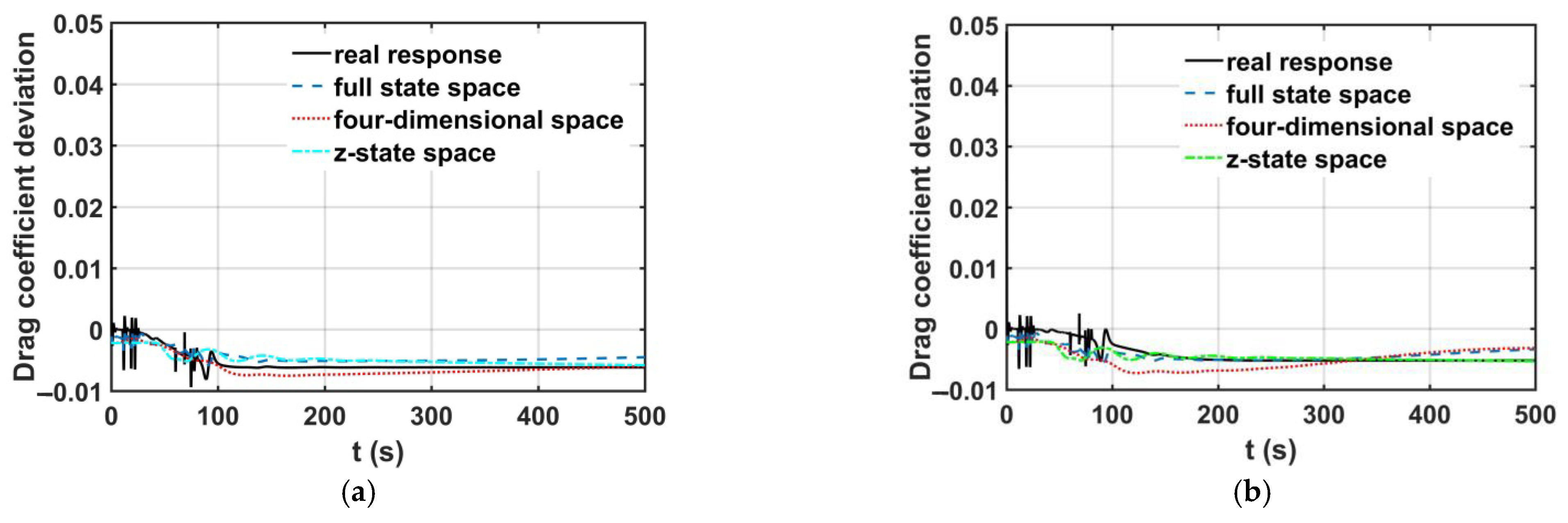
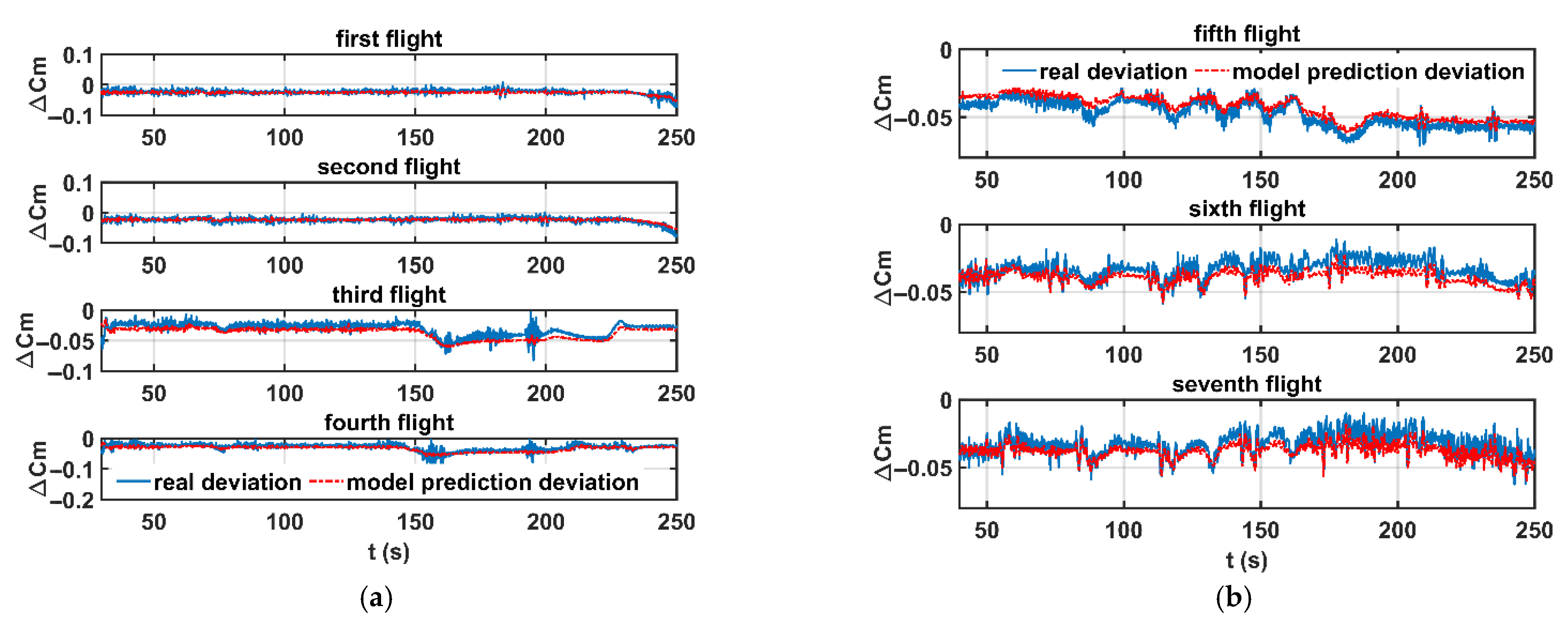
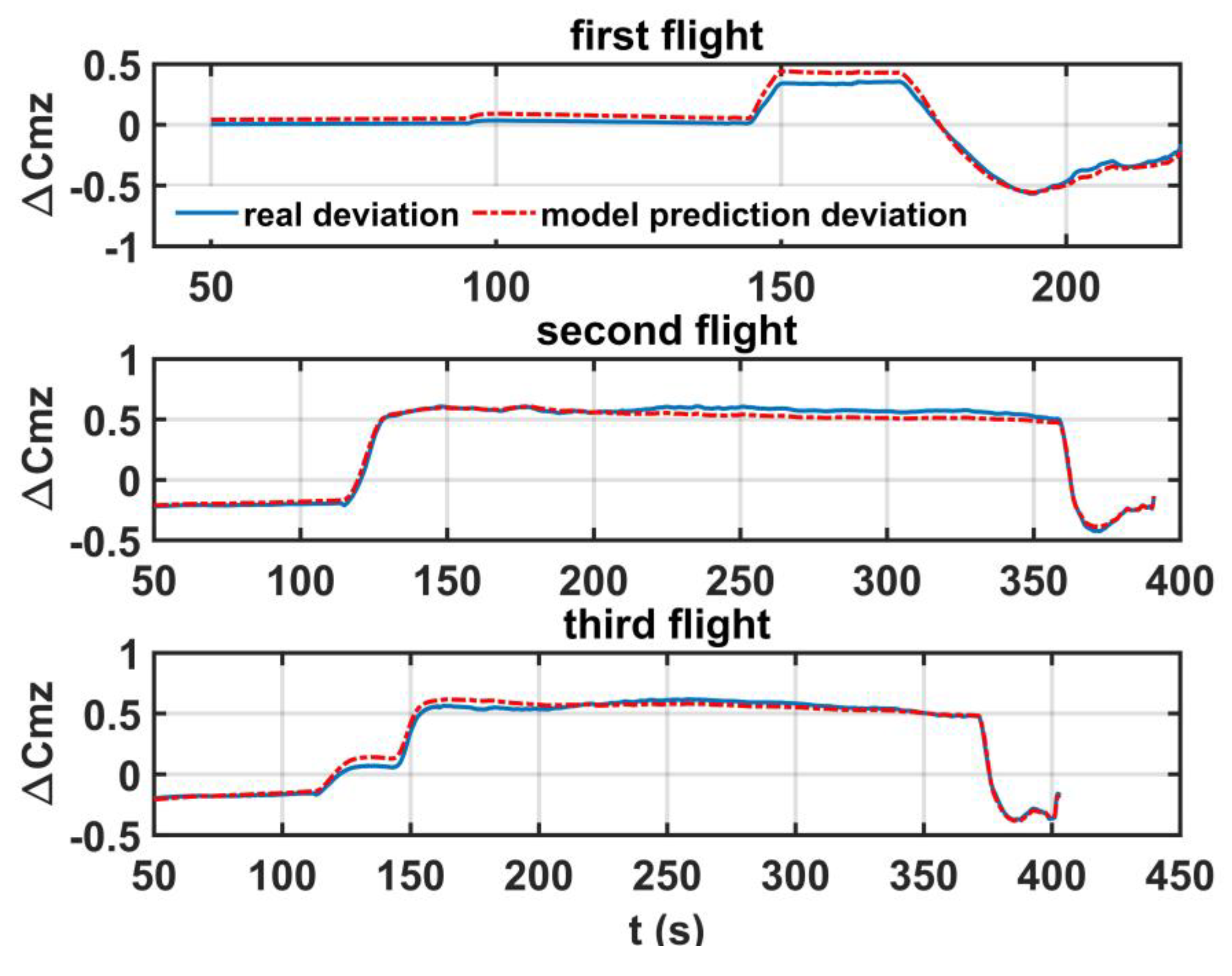
The paper discusses data analysis and modeling for studying the aerodynamic characteristics correlation between ground and flight of aerospace vehicles. The paper explores the feasibility and effectiveness of symbolic regression and the NCA method in modeling the physical correlation for ground-to-flight deviations of aerodynamic coefficients in high dimensional flight state space. Simulation examples validate the symbolic regression toolbox GPSR and NCA method. Then, the tool and the method are applied to model the aerodynamic ground-to-flight deviation of pitching moment coefficients existing in the actual flight test data of a UAV and an XRLV. The paper compares the prediction accuracy of the spatial dimensionality reduction-based symbolic regression for actual flight tests with three typical data-driven models and demonstrates its successful application in finite flight test data modeling. The mathematical model delivers a multi-fold enhancement in fitting accuracy over data-driven methods for all fight cases. For UAV flight test data, the RMSE of the mathematical model demonstrates a maximum improvement of 37% in accuracy compared to three data-driven methods. For XRLV flight test data, the prediction accuracy of the mathematical model shows an enhancement exceeding 80% relative to Gaussian kernel SVM and Gaussian process data-driven models.
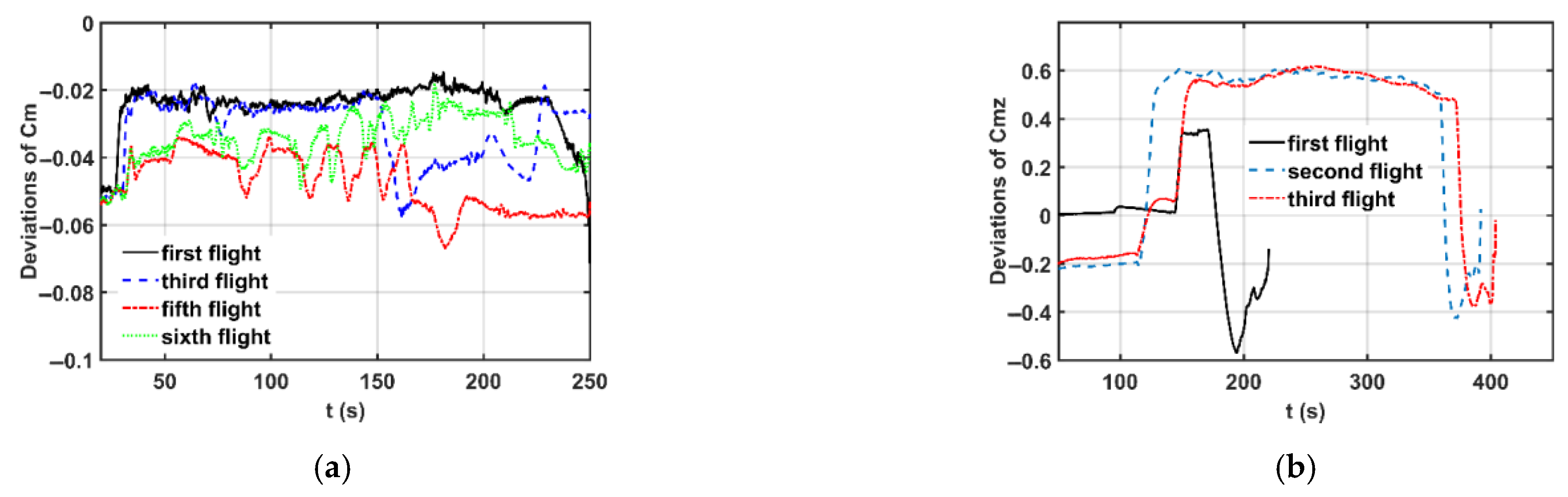
The study establishes that flow similarity plays a significant role in the vehicle’s aerodynamic characteristics correlation between ground and flight. Due to wall interference and blockage effects in ground wind tunnel tests, the aerodynamic characteristics of aerospace vehicles in the testing environment differ significantly from those under real atmospheric conditions, and simple wall interference corrections cannot fully eliminate the ground-to-flight discrepancies. Because of the internal physical connection between the multiple flight test data with the ground test data of the same type of vehicle, the modeling methodology can dig out a similar physical law in aerodynamic ground-to-flight deviations despite different flight conditions. For the pitching moment coefficient deviations between flight and ground, the methodology proposed in this paper ultimately establishes two similar mathematical models solely related to the angle of attack for two distinct vehicle configurations. Physically, the angle of attack is one of the most significant state variables affecting the aerodynamic characteristics of aerospace vehicles in pitch motion, and it also serves as a critical factor in ground wind tunnel experiments for investigating aerodynamic characteristics. The mathematical models developed through the symbolic regression methodology in this study effectively reveal the physical principles governing the influence of angle of attack on pitching moment coefficient deviations under different testing conditions.
This paper aims to combine the data feature extraction method with symbolic regression to mine aerospace vehicles’ aerodynamic ground-to-flight deviation laws. These methods show an application prospect for similar data modeling problems with limited data samples and strong physical correlations. However, when the assumptions of flow similarity and intrinsic physical connections are not satisfied, this methodology may fail. Additionally, the limitations of symbolic regression-based approaches, including computational inefficiency and reduced interpretability of results caused by inherent randomness, also exist in this methodology. The methods have only been applied to model typical flight scenarios for two types of vehicles. Subsequently, the application of the methods is anticipated to be expanded to encompass a wider variety of aerospace vehicle types and a broader spectrum of highly nonlinear flight scenarios, including large-angle-of-attack maneuvers, tailspin rotations, in-flight system failures, and hypersonic flight conditions. Modeling and analysis of data physical laws can be further developed to address these problems and extreme cases.

Author Contributions

Conceptualization, D.D.; data curation, Q.C.; formal analysis, D.D.; investigation, Q.W.; software, Q.C.; supervision, Q.W.; validation, D.D.; writing—original draft, D.D.; writing—review and editing, L.H. All authors have read and agreed to the published version of the manuscript.

Funding

This research received no external funding.

Data Availability Statement

The datasets used during the current study are available from the corresponding author on reasonable request.

Acknowledgments

The model flight team of the China Aerodynamics Research and Development Centre provided the flight test data for this article.

Conflicts of Interest

The authors declare no conflicts of interest.

Abbreviations

The following abbreviations are used in this manuscript:
NCANeighborhood component analysis
SRSymbolic regression
AOAAngle of attack
CFDComputational fluid dynamics
SVMSupport vector machine
GPGenetic programming
GPSRGP-based symbolic regression
KNNK-nearest neighbors
RMSERoot mean square error
UAVUnmanned aerial vehicle
XRLVX-rudder layout vehicle

References

  1. Pettersson, K.; Rizzi, A. Aerodynamic scaling to free flight conditions: Past and present. Prog. Aerosp. Sci. 2008, 44, 295–313. [Google Scholar] [CrossRef]
  2. Bushnell, D.M. Scaling: Wind tunnel to flight. Ann. Rev. Fluid Mech. 2006, 38, 111–128. [Google Scholar] [CrossRef]
  3. Tai, S.; Bu, C.; Wang, Y.; Yue, T.; Liu, H.; Wang, L. Identification of aircraft longitudinal aerodynamic parameters using an online corrective test for wind tunnel virtual flight. Chin. J. Aeronaut. 2024, 37, 261–275. [Google Scholar] [CrossRef]
  4. Tumse, S.; Bilgili, M.; Sahin, B. Estimation of aerodynamic coefficients of a non-slender delta wing under ground effect using artificial intelligence techniques. Neural Comput. Appl. 2022, 34, 10823–10844. [Google Scholar] [CrossRef]
  5. Chen, Z.; Xue, F.; Yu, H.; Wang, Y.; Jiang, Z.; Lu, W.; Dong, L. Derivation and validation of a similarity law for free-flight wind tunnel tests of parallel stage separation. Chin. J. Aeronaut. 2023, 36, 91–100. [Google Scholar] [CrossRef]
  6. Xue, F.; Wang, H.; Jiang, Z.; Wang, Y. Derivation and verification of a similarity law for wind-tunnel free-flight tests of heavy-store separation. Acta Astronaut. 2020, 174, 123–130. [Google Scholar] [CrossRef]
  7. Liu, Z.; Yang, W.; Shen, Q. Investigation on correlation between wind tunnel and flight test data for boundary layer transition. In Proceedings of the AIAA Flight Testing Conference, Washington, DC, USA, 13–17 June 2016; AIAA: Reston, VA, USA, 2016. [Google Scholar] [CrossRef]
  8. Schneider, S.P. Developing mechanism-based methods for estimating hypersonic boundary-layer transition in flight: The role of quiet tunnels. Prog. Aerosp. Sci. 2015, 72, 17–29. [Google Scholar] [CrossRef]
  9. Schwartz, N.J.; Gudmundsson, S.; Oliveira, G.; Wayman, T.R.; Mosedale, A. Investigation of wind tunnel support system interference on a business jet aircraft model at transonic conditions using computational fluid dynamics. In Proceedings of the AIAA SCITECH 2024 Forum, Orlando, FL, USA, 8–12 January 2024; AIAA: Reston, VA, USA, 2024. [Google Scholar] [CrossRef]
  10. Bertram, A.; Hoffmann, N.; Goertz, S.; Gebbink, R.; Janssen, S.R. An alternative wind tunnel data correction based on CFD and experimental data in the transonic flow regime. In Proceedings of the AIAA Aviation 2021 Forum, Virtual, 2–6 August 2021; AIAA: Reston, VA, USA, 2021. [Google Scholar] [CrossRef]
  11. Niu, J.Q.; Zhou, D.; Liang, X.F.; Liu, S.; Liu, T.-H. Numerical simulation of the Reynolds number effect on the aerodynamic pressure in tunnels. J. Wind Eng. Ind. Aerodyn. 2018, 173, 187–198. [Google Scholar] [CrossRef]
  12. Wang, Q.; He, K.-F.; Qian, W.-Q.; Zhang, T.-J.; Cheng, Y.-Q.; Wu, K.-Y. Unsteady aerodynamics modeling for flight dynamics application. Acta Mech. Sin. 2012, 28, 14–23. [Google Scholar] [CrossRef]
  13. Wang, Q.; Qian, W.Q.; He, K.F. Unsteady aerodynamic modeling at high angles of attack using support vector machines. Chin. J. Aeronaut. 2015, 28, 659–668. [Google Scholar] [CrossRef]
  14. Roudbari, A.; Saghafi, F. Intelligent modeling and identification of aircraft nonlinear flight. Chin. J. Aeronaut. 2014, 27, 759–771. [Google Scholar] [CrossRef]
  15. Ghazi, G.; Bosne, M.; Sammartano, Q. Cessna citation X stall characteristics identification from flight data using Neural Networks. In Proceedings of the AIAA Atmospheric Flight Mechanics Conference, Grapevine, TX, USA, 9–13 January 2017; AIAA: Reston, VA, USA, 2017. [Google Scholar] [CrossRef]
  16. Jategaonkar, R.; Fischenberg, D.; von Gruenhagen, W. Aerodynamic modeling and system identification from flight data recent applications at DLR. J. Aircr. 2004, 41, 681–691. [Google Scholar] [CrossRef]
  17. Deiler, C. Aerodynamic modeling, system identification and analysis of iced aircraft configurations. In Proceedings of the AIAA Atmospheric Flight Mechanics Conference, Washington, DC, USA, 13–17 June 2016; AIAA: Reston, VA, USA, 2016. [Google Scholar] [CrossRef]
  18. Deiler, C. Time-domain output error system identification of iced aircraft aerodynamics. CEAS Aeronaut. J. 2017, 8, 231–244. [Google Scholar] [CrossRef]
  19. Deiler, C.; Kilian, T. Dynamic aircraft simulation model covering local icing effects. CEAS Aeronaut. J. 2018, 9, 429–444. [Google Scholar] [CrossRef]
  20. Luo, C.T.; Zhang, S.L. Parse-matrix evolution for symbolic regression. Eng. Appl. Artif. Intell. 2012, 25, 1182–1193. [Google Scholar] [CrossRef]
  21. Luo, C.; Hu, Z.; Zhang, S.-L.; Jiang, Z. Adaptive space transformation: An invariant based method for predicting aerodynamic coefficients of hypersonic vehicles. Eng. Appl. Artif. Intell. 2015, 46, 93–103. [Google Scholar] [CrossRef]
  22. Koza, J.R. Genetic programming as a means for programming computers by natural selection. Stat. Comput. 1994, 4, 87–112. [Google Scholar] [CrossRef]
  23. Iba, H.; DeGaris, H.; Sato, T. A numerical approach to genetic programming for system identification. Evol. Comput. 1995, 3, 417–452. [Google Scholar] [CrossRef]
  24. McKay, B.; Willis, M.; Barton, G. Steady-state modelling of chemical process systems using genetic programming. Comput. Chem. Eng. 1997, 21, 981–996. [Google Scholar] [CrossRef]
  25. Patil-Shinde, V.; Tambe, S.S. Genetic programming based models for prediction of vapor-liquid equilibrium. Calphad 2018, 60, 68–80. [Google Scholar] [CrossRef]
  26. Balasubramaniam, P.; Kumar, A.V.A. Solution of matrix Riccati differential equation for nonlinear singular system using genetic programming. Genet. Program. Evol. Mach. 2008, 10, 71–89. [Google Scholar] [CrossRef]
  27. Quade, M.; Abel, M.; Shafi, K.; Niven, R.K.; Noack, B.R. Prediction of dynamical systems by symbolic regression. Phys. Rev. E 2016, 94, 012214. [Google Scholar] [CrossRef] [PubMed]
  28. Gaucel, S.; Keijzer, M.; Lutton, E.; Tonda, A. Learning dynamical systems using standard symbolic regression. In Proceedings of the European Conference on Genetic Programming, LNTCS, Granada, Spain, 23–25 April 2014; Volume 8599. [Google Scholar] [CrossRef]
  29. Moreno-Salinas, D.; Besada-Portas, E.; López-Orozco, J.A.; Chaos, D.; de la Cruz, J.; Aranda, J. Symbolic regression for marine vehicles identification. IFAC-PapersOnLine 2015, 48, 210–216. [Google Scholar] [CrossRef]
  30. Schmidt, M.; Lipson, H. Distilling free-form natural laws from experimental data. Science 2009, 324, 81–85. [Google Scholar] [CrossRef]
  31. O’Neill, M.; Ryan, C. Grammatical evolution. IEEE Trans. Evol. Comput. 2001, 5, 349–358. [Google Scholar] [CrossRef]
  32. França, F.O. A greedy search tree heuristic for symbolic regression. Inf. Sci. 2018, 442, 18–32. [Google Scholar] [CrossRef]
  33. Cozad, A.; Sahinidis, N.V. A global MINLP approach to symbolic regression. Math. Program. Ser. B 2018, 170, 97–119. [Google Scholar] [CrossRef]
  34. Petersen, B.K.; Landajuela, M.; Mundhenk, T.N.; Santiago, C.P.; Kim, S.K.; Kim, J.T. Deep symbolic regression: Recovering mathematical expressions from data via risk-seeking policy gradients. arXiv 2021, arXiv:1912.04871. [Google Scholar] [CrossRef]
  35. Makke, N.; Chawla, S. Interpretable scientific discovery with symbolic regression: A review. Artif. Intell. Rev. 2024, 57, 2. [Google Scholar] [CrossRef]
  36. Goldberger, J.; Roweis, S.; Hinton, G.; Salakhutdinov, R. Neighbourhood components analysis. In Proceedings of the 18th International Conference on Neural Information Processing Systems, Vancouver, BC, Canada, 13–18 December 2004; Volume 17, pp. 513–520. [Google Scholar]
  37. Yang, Z.; Laaksonen, J. Regularized neighborhood component analysis. In Proceedings of the 15th Scandinavian Conference on Image Analysis, SCIA 2007, Aalborg, Denmark, 10–14 June 2007. [Google Scholar] [CrossRef]
  38. Zheng, Y.; Liu, Q.; Chen, E.; Zhao, J.L.; He, L.; Lv, G. Convolutional nonlinear neighbourhood components analysis for time series classification. In Proceedings of the Advances in Knowledge Discovery and Data Mining, Ho Chi Minh City, Vietnam, 19–22 May 2015; Lecture Notes in Computer Science. Volume 9078, pp. 534–546. [Google Scholar] [CrossRef]
  39. Qin, C.; Song, S.; Huang, G.; Zhu, L. Unsupervised neighborhood component analysis for clustering. Neurocomputing 2015, 168, 609–617. [Google Scholar] [CrossRef]
  40. Raghu, S.; Sriraam, N. Classification of focal and non-focal EEG signals using neighborhood component analysis and machine learning algorithms. Expert Syst. Appl. 2018, 113, 18–32. [Google Scholar] [CrossRef]
  41. Melody, J.W.; Başar, T.; Perkins, W.R.; Voulgaris, P. Parmeter identification for inflight detection and characterization of aircraft icing. Control Eng. Pract. 2000, 8, 985–1001. [Google Scholar] [CrossRef]
Figure 1. GPSR toolkit interface.
Aerospace 12 00455 g001
Figure 2. The impact analysis on the drag coefficient deviation for Twin Otter simulation data. (a) Single flight data analysis, different colors and marks represent the different flight tests displayed in the horizontal coordinate; (b) all cases of flight data analysis.
Aerospace 12 00455 g002
Figure 3. Comparison of SVM predictors with Twin Otter response data. (a) Fifth flight prediction results; (b) eighth flight prediction results.
Aerospace 12 00455 g003
Figure 4. Root mean square deviations of UAV and XRLV’s aerodynamic coefficients. (a) deviations of seven UAV flights; (b) deviations of three XRLV flights.
Aerospace 12 00455 g004
Figure 5. Deviations of UAV and XRLV pitching moment coefficients in flight tests. (a) UAV flight tests; (b) XRLV flight tests.
Aerospace 12 00455 g005
Figure 6. The impact analysis on pitching moment coefficient deviation for UAV flight data. (a) data analysis of single flight test, different colors and marks represent the different flight tests displayed in the horizontal coordinate; (b) data analysis of all flight tests.
Aerospace 12 00455 g006
Figure 7. The impact analysis on pitching moment coefficient deviation for XRLV flight data. (a) Data analysis of single flight test, different colors and marks represent the different flight tests displayed in the horizontal coordinate; (b) data analysis of all flight tests.
Aerospace 12 00455 g007
Figure 8. Mathematical model predictions for UAV flight tests. (a) Forecast results for the first to the fourth flight tests; (b) forecast results for the fifth to seventh flight tests.
Aerospace 12 00455 g008
Figure 9. Mathematical model predictions for XRLV flight tests.
Aerospace 12 00455 g009
Table 1. Performance of GPSR tool.
No.DimFormulaSolutionDomainRMSE
11 x 2 + 0.5 x 1 x 2 + 0.5 x 1.002 [−1, 1]1.72 × 10⁻³
21 s i n x c o s x + e x p x e x p x + s i n x c o s x [−1, 1]0
32 x 0 2 + 0.7 x 0 1 / x 1 x 0 + 0.3418 2 1.091 / x 1 [0.5, 2.5]28.94 × 10⁻³
42 l n x 0 + x 1 s i n x 0 s i n l n x 0 + x 1 s i n x 0 + 0.02 [0.5, 2.5]22.55 × 10⁻²
53 x 0 2 x 0 x 2 + x 1 x 2 x 2 2 + 0.5 x 0 2 x 0 x 2 + x 1 x 2 x 2 2 + 0.4513 [−1, 1]34.87 × 10⁻²
63 x 0 1 s i n x 1 c o s x 2 x 0 1 s i n x 1 c o s x 2 [0.2, 2.2]30
Note: The superscript of the parameter value range in Domain denotes the spatial dimension of the independent variable.
Table 2. Labeling of state-space variables of Twin Otter aircraft.
Serial No.1~34~67~910~12131415~17
State variablesVelocity components in the body coordinateAngular velocity components in the body coordinatePitch, yaw and roll anglesPosition in the inertial coordinateAOASideslip angleAileron, elevator and rudder deflection angles
Table 3. Comparison of SVM predictors’ RMSE for the Twin Otter simulation data.
State Space Selection1st Flight2nd Flight3rd Flight4th Flight5th Flight6th Flight7th Flight8th Flight
Full state space8.73 × 10−42.8 × 10−31.7 × 10−31.8 × 10−31.4 × 10−32.8 × 10−31.4 × 10−31.4 × 10⁻³
Four-dimensional state space1.1 × 10−32.8 × 10−32.0 × 10−32.1 × 10−31.2 × 10−31.9 × 10−32.5 × 10−32.2 × 10⁻³
z-state space1.4 × 10−32.8 × 10−32.5 × 10−32.1 × 10−31.4 × 10−33.1 × 10−31.6 × 10−31.5 × 10⁻³
Table 4. Labeling of state variables of the UAV flight tests.
Serial No.1~34~67~910~12131415~20
State variablesVelocity components in the inertial coordinateAngular velocity components in the body coordinateYaw, pitch and roll anglesPosition in the inertial coordinateAOASideslip angleControl surface deflection angles
Serial No.2122~2526272829
State variablesMassMoment of inertias and product of inertiaEngine thrustWing reference areaMean aerodynamic chordWing span
Table 5. Labeling of state variables of the XRLV flight tests.
Serial No.1~34~67~910~121314~16
State variablesVelocity components in the inertial coordinateAngular velocity components in the body coordinatePitch, yaw and roll anglesPosition in the inertial coordinateAOAPitch, yaw, and roll channel deflection angles
Serial No.1718~20212223
State variablesMassMoment of inertiasReference areaReference lengthMach number
Table 6. Accuracy of ground-to-flight deviation models for UAV flight test data.
RMSE1st Flight2nd Flight3rd Flight4th Flight5th Flight6th Flight7th FlightAverage
Mathematical model0.00850.00850.01020.01010.00950.00950.00930.0094
Squared kernel SVM0.00460.00360.01910.01590.01830.02240.02110.015
Gaussian kernel SVM0.00480.00350.0090.00950.01530.01280.01090.0094
Gaussian process model0.00420.00120.01370.01210.00750.01820.01630.0105
Table 7. Accuracy of ground-to-flight deviation models for XRLV flight test data.
RMSE1st Flight2nd Flight3rd FlightAverage
Mathematical model0.05200.03760.03450.0414
Squared kernel SVM6.19 × 10116.11 × 10110.03374.1 × 1011
Gaussian kernel SVM0.23550.53510.02860.2664
Gaussian process model0.20140.46534.34 × 10−40.2224
Disclaimer/Publisher’s Note: The statements, opinions and data contained in all publications are solely those of the individual author(s) and contributor(s) and not of MDPI and/or the editor(s). MDPI and/or the editor(s) disclaim responsibility for any injury to people or property resulting from any ideas, methods, instructions or products referred to in the content.

