On Dynamics of a Copter-Slung Spherical Payload Partially Filled with Liquid

Abstract

The motion of a copter with a suspended payload in a vertical plane is considered. The payload has a spherical shape and contains a concentric spherical cavity partially filled with ideal liquid. The system is subjected to horizontal stationary wind. The aerodynamic load on the payload is described within the framework of a quasi-steady approach. The dynamics of the liquid are simulated using the phenomenological pendulum model. The points of this study are the controllability and observability of a stationary flight of a copter with the payload. A control strategy is proposed, which aims to bring the system from a certain initial state to a certain final state, such that the center of mass of the copter moves along a given sufficiently smooth curve. The control is designed to ensure the suppression of oscillations of the payload and the liquid along the entire trajectory.

1. Introduction

Studies on the dynamics of suspended loads and the development of effective control laws have high practical importance for various fields (in particular, in connection with the manipulation of loads using cranes, when transporting loads using helicopters or copters, etc.). As a rule, mechanical systems that arise in this case are underactuated. The goal of control is usually to deliver the load to a given end point (often along a given trajectory) and suppress load oscillations. An extensive body of the literature is devoted to the construction of appropriate control laws, for example, the damping of oscillations of a payload manipulated by a crane, which is discussed in [1,2,3]. In addition, various algorithms for controlling the motion of a helicopter carrying a load on a cable are proposed in [4,5,6].

A review of the current state of research in the field of controlling a quadcopter with a suspended load is given in papers by Omar H.M. et al. and Estevez J. et al. [7,8]. When controlling a quadcopter with a suspended load, the main tasks are tracking the target trajectory (this can be the trajectory of the copter and/or the trajectory of the load), as well as damping the oscillations of the load. Various control strategies have been developed to solve these problems (e.g., [9,10,11,12]), including in conditions of insufficient information about the mass of the load [13]. A number of studies have performed more or less detailed modeling of the dynamics of the behavior of the cable, taking into account its elastic properties and/or flexibility [14,15].

A separate area of research is the construction of control algorithms for cooperative transportation of payload by several copters, which can be found in [16,17].

In most studies, aerodynamic forces acting on the load are not taken into account, or they are considered as a disturbance. However, in the case when the load is lightweight and its surface area is large enough (so that the aerodynamic force is comparable with the gravity force), it seems reasonable to consider the aerodynamic load in more detail. Bisgaard et al. and Sun et al. assumed that the aerodynamic load is reduced to the drag force [18,19]. Holub et al. [20] considered the situation when, along with the drag force, there is a lateral force, and analyzed the possibility of constructing a control that ensures robust stabilization of vertical ascent and descent under conditions of incomplete information about these effects.

In real situations, the load can have fairly complex structure. For example, it can contain a cavity partially filled with liquid. Fluctuations of the liquid can have a noticeable effect on the behavior of the load, and this should be taken into account when constructing the control.

The start of active research into fluid oscillations in a cavity was associated with the need to model oscillations of fuel in the tanks of space rockets. Analysis of such in a full hydrodynamic formulation is a rather complex problem. Therefore, numerous studies have been aimed at finding simplified approaches.

Okhotsimskii [21] considered a system that represented a body with a cavity in the form of a cylinder (or two coaxial cylinders), partially filled with an ideal liquid. He had shown that for certain types of motion, there were three independent inertial characteristics of the system, and a method for calculating them was developed.

Abramson et al. [22] proposed a simplified mechanical model representing a system of oscillators intended to describe the forces acting on a partially filled cylindrical tank from the liquid oscillating in it.

A body with a spherical cavity partially filled with liquid was considered in papers by Stofan et al., Abramson et al., and Chu [23,24,25]. The results of calculations (under the assumption that the liquid performs a potential irrotational flow) and experiments to determine the natural frequencies of oscillations of the liquid were presented. Summer provided experimental data on the identification of the parameters of a pendulum simulating oscillations of a liquid [26].

Aliabadi et al. [27] investigated oscillations of liquid in a horizontal cylindrical tank and showed that the results obtained within the framework of the pendulum model agree quite well with the results obtained by hydrodynamic modeling if the degree of filling of the tank is less than one half. Godderidge et al. [28] described the oscillations of the liquid using a modified pendulum model, which allows for, among other things, simulating the impacts of the liquid on the walls of the vessel. Moriello et al. [29] studied the problem of moving a cylindrical vessel partially filled with liquid using a manipulator along a given trajectory without exciting oscillations of the liquid. The motion of the liquid is modeled using a spherical pendulum, the suspension point of which is located at the intersection of the cavity axis with the unperturbed surface of the liquid. Alshaya et al. [30] proposed a smooth polynomial-shaped control law with an adjustable command time length intended to eliminate the residual vibration of liquid in a container. The liquid dynamics were described with a series of oscillators.

Sayyaadi et al. [31] considered the problem of transporting a tank partially filled with liquid using several copters (the aerodynamic impact on the load is not taken into account). It was shown that three copters can stabilize the target motion and dampen oscillations of the tank and liquid. A method for controlling a copter with a liquid tank suspended with two cables was proposed by Zhu et al. [32]. They considered the aerodynamic load on the tank a disturbance.

The present paper considers the motion of a quadcopter with a slung spherical load that contains a spherical cavity partially filled with ideal liquid. The aerodynamic drag acting on the load is taken into account (including the load that is caused by the wind). Oscillations of liquid inside the cavity are simulated using a modified pendulum model. A strategy is proposed for controlling the thrust forces of the copter propellers in order to ensure tracking of a given trajectory (provided that it is sufficiently smooth) and prevention of large oscillations of the liquid inside the cavity.

2. Materials and Methods

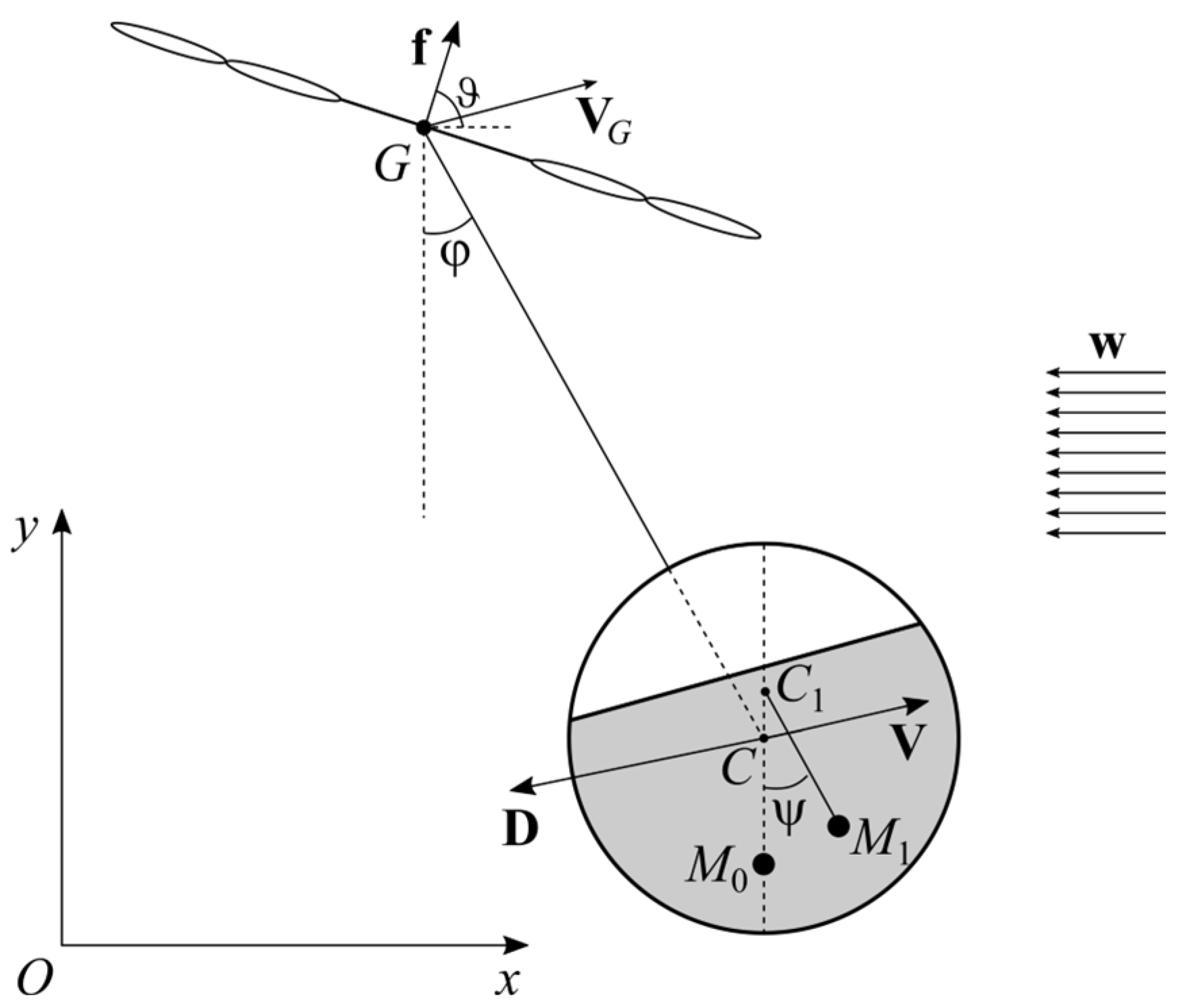
We consider a mechanical system consisting of a copter and a load. The load has a spherical shape and is slung to the center of mass G of the copter with an inextensible weightless string. The center of mass of the load (denoted as C) is located in the center of the spherical shell. Inside the load, there is a spherical cavity with the center in C. The cavity is partially filled with ideal fluid (Figure 1).

The system is subjected to wind flow with a constant w wind speed. We restrict our consideration to the case when the system moves in the vertical plane parallel to the wind velocity. Let system O_xy (shown in Figure 1) be the reference frame in this plane, where the O_y axis is directed vertically upwards and the O_x axis is directed against the wind.

We assume that the central moment of inertia of the copter is very small, so that one can neglect the dynamics of rotational motion of the copter with respect to its center of mass.

In order to describe the position of the copter and the load, we introduce the following generalized coordinates: x_G and y_G denote the coordinates center of mass (G) in the O_xy reference frame while φ denotes the angle between the string and the vertical axis.

Suppose that the aerodynamic load upon the slung body can be reduced to the drag force D, for which the following formula holds [33]:

$$D=-{\displaystyle \frac{\rho S}{2}}V{C}_{d}V,$$

(1)

where ρ is the air density, S is the characteristic area, V is the flow velocity vector relative to the center C of the load, and C_d is the non-dimensional drag coefficient. As shown in [34] (p. 24), the dependence of this coefficient on the Reynolds number is quite weak in a wide range of Reynolds numbers (from 10³ to 10⁵, which covers the common range of copter speeds). In subsequent simulations, based on data from [34], we used C_d = 0.45.

Copter rotors generate downwash that, in principle, can contribute to the aerodynamic forces acting on the payload. However, wind tunnel measurements (e.g., [35]) show that, in the presence of wind (even rather low, about 2.5 m/s), the effect of the induced velocity becomes practically negligible at distances of about 2 rotor diameters. This is primarily due to the fact that the downwash is “blown” by the wind. The same holds for the case when the horizontal speed of the copter is not too low. In what follows, we suppose that the distance $GC$ is large and the horizontal component of the flow velocity $V$ is high. Then, it is reasonable to neglect the downwash effect. The situation when the horizontal component of the flow speed is low needs additional consideration, which remains for future research.

Flow velocity (V) can be given by the following equality:

$$V=\sqrt{{\left(\dot{x}+l\dot{\phi }\cos \phi +w\right)}^2+{\left(\dot{y}+l\dot{\phi }\sin \phi \right)}^2}.$$

(2)

Here, $w$ is the wind speed.

In order to describe the dynamics of the fluid inside the cavity, we act by the analogy of the “pendulum” approach described in [29,36]. In the context of this approach, the fluid is divided into two parts: one of them remains steady with respect to the cavity, and the other one oscillates with respect to it. In order to describe the dynamics of the second part, a series of mathematical pendulums are used. Strictly speaking, the number of pendulums should be infinite; however, in many cases, the effect of the majority of pendulums on the dynamics of the entire system is low, and only several of them are taken into account (or even one). In this approach, it is supposed that the container performs small oscillations near the vertical position (φ = 0).

However, for of container, which is slung to a copter, the situation can be different. Due to the presence of the aerodynamic force, the container will change its angles with the vertical when the copter performs steady horizontal flight with different speeds (generally speaking, these angles might be rather large). The fluid in steady state will take the position where its potential energy is minimum. Nevertheless, this position depends on the position of the container. Therefore, it seems impossible to pick a part of fluid that would remain immobile with respect to the cavity in wide enough range of flight speeds. In order to eliminate this issue, we modify the pendulum approach as follows:

We subdivide the fluid into two parts: one that remains steady and the one that oscillates. We assume that the first part performs a “quasi-steady” motion, i.e., it always takes the position corresponding to the equilibrium for the current state of motion of the container. This means that its center of mass of the quasi-steady fluid (denoted as M₀) always lies on the vertical axis, and it always passes through C (below this point). We denote the mass of this part of the fluid with m₀, and the CM₀ distance with l₀ (Figure 2).

We simulate the behavior of the “oscillatory” part by using the mathematical pendulum M₁ (so to speak, “liquid pendulum”) with a length l₁ and mass m₁. The pivot point C₁ lies on the vertical line, which passes through the center of the cavity C, and CC₁ = h₁. The angle of displacement of this pendulum from the vertical axis is denoted with ψ (one more generalized coordinate).

The length l₁ of the “liquid pendulum” is determined in such a way that the natural frequency of the oscillator coincides with the frequency of the first oscillation mode of the fluid in the cavity near the equilibrium. This value, as well as parameters h₁ and m₁, should be identified based on results of experiments or hydrodynamic simulation of oscillations of fluid in a cavity.

In order to calculate values m₀ and l₀, we use the following considerations: Let the system be in equilibrium (see Figure 2). First, we introduce the following notations: R is the cavity radius; h is the distance from the lowest point of the cavity to the fluid surface level; m_l and ρ_l are fluid mass and density; ∆y is the difference between the ordinate of the center of mass C_l of the fluid and the ordinate of point C (evidently, ∆y ≤ 0). One can readily see that the following relations hold:

$$\begin{array}{l}{m}_l=m_0+m_1={\rho }_l{\displaystyle \frac{\pi h^2}{3}}\left(3R-h\right),\hspace{1em}\\ m_l\Delta y=-m_0{l}_0+m_1(h_1-l_1)=-{\rho }_l{\displaystyle \frac{\pi h^2{\left(2R-h\right)}^2}{4}}.\end{array}$$

(3)

From (1), it follows that, given m₁, l₁, and h₁, the values m₀ and l₀ can be determined uniquely.

The “liquid” oscillator moves under the action of gravity and inertia forces only; no damping is introduced because we consider the case of ideal fluid.

Taking into account the above, the system under consideration has four degrees of freedom. We write down the equations of motion in form of the Lagrange equations of the second kind. Kinetic (T) and potential (П) energy of the system are given by the following formulas:

$$\begin{array}{l}T={\displaystyle \frac{\left(m_c+m+m_0+m_1\right)\left({\dot{x}}^2+{\dot{y}}^2\right)}{2}}+{\displaystyle \frac{\left(J+\left(m+m_0+m_1\right)l^2\right){\dot{\phi }}^2}{2}}+{\displaystyle \frac{m_1{l}_1^2{\dot{\psi }}^2}{2}}\\ +\left(m+m_0+m_1\right)l\dot{\phi }\left(\dot{x}\cos \phi +\dot{y}\sin \phi \right)+m_1{l}_1\dot{\psi }\left(l\dot{\phi }\cos (\psi -\phi )+\dot{x}\cos \psi +\dot{y}\sin \psi \right),\\ \Pi =m_{c}gy+\left(m+m_0+m_1\right)g\left(y-l\cos \phi \right)-m_{1}g{l}_1\cos \psi .\end{array}$$

(4)

Here, m_c is the copter mass, m is the container mass (without the fluid), J is the central moment of inertia of the fluid, l is the distance between the centers of masses of the copter and the container, and g is the gravity acceleration.

The equations of motion are as follows:

$$\begin{array}{l}{\displaystyle \frac{d}{dt}}{\displaystyle \frac{\mathit{\partial }T}{\mathit{\partial }\dot{x}}}={ℱ}_x,\\ {\displaystyle \frac{d}{dt}}{\displaystyle \frac{\mathit{\partial }T}{\mathit{\partial }\dot{y}}}+{\displaystyle \frac{\mathit{\partial }\Pi }{\mathit{\partial }y}}={ℱ}_y,\\ {\displaystyle \frac{d}{dt}}{\displaystyle \frac{\mathit{\partial }T}{\mathit{\partial }\dot{\phi }}}-{\displaystyle \frac{\mathit{\partial }T}{\mathit{\partial }\phi }}+{\displaystyle \frac{\mathit{\partial }\Pi }{\mathit{\partial }\phi }}={ℱ}_{\phi },\\ {\displaystyle \frac{d}{dt}}{\displaystyle \frac{\mathit{\partial }T}{\mathit{\partial }\dot{\psi }}}-{\displaystyle \frac{\mathit{\partial }T}{\mathit{\partial }\psi }}+{\displaystyle \frac{\mathit{\partial }\Pi }{\mathit{\partial }\psi }}={ℱ}_{\psi },\end{array}$$

(5)

where F_x, F_y, F_φ, and F_ψ are the corresponding generalized forces.

In order to reduce the number of parameters and somewhat simplify the subsequent analysis, we normalize the equations of motion (5). For that, we choose characteristic time equal to $\sqrt{l/g}$, characteristic mass equal to $m+m_l$ (mass of the payload together with the fluid), and characteristic length equal to l (which equals to the earlier defined distance between the centers of masses). Hereinafter, we hold the old notations for dimensionless parameters and variables and denote the derivative with respect to the dimensionless time $\tau =t\sqrt{g/l}$ with a dot. Additionally, we introduce the following dimensionless parameter:

$$\mu ={\displaystyle \frac{\rho Sl{C}_d}{2\left(m+m_l\right)}}.$$

(6)

Then, taking into account (1), (2), (4), and (6), the normalized equations of dynamics of the system can be written down as follows:

$$M\ddot{X}=F+U,$$

(7)

where

$$\begin{array}{l}X={\left(\begin{array}{cccc}x& y& \phi & \psi \end{array}\right)}^T,\hspace{1em}U={\left(\begin{array}{cccc}f\cos \vartheta & f\sin \vartheta & 0& 0\end{array}\right)}^T,\\ M=\left(\begin{array}{cccc}{m}_c+1& 0& \cos \phi & m_1{l}_1\cos \psi \\ 0& m_c+1& \sin \phi & m_1{l}_1\sin \psi \\ \cos \phi & \sin \phi & J+1& m_1{l}_1\cos (\phi -\psi )\\ m_1{l}_1\cos \psi & m_1{l}_1\sin \psi & m_1{l}_1\cos (\phi -\psi )& m_1{l}_1^2\end{array}\right),\\ F=\left(\begin{array}{c}-\mu V_{x}V-{\dot{\phi }}^2\sin \phi -m_1{l}_1{\dot{\psi }}^2\sin \psi \\ -\mu V_{y}V-{\dot{\phi }}^2\cos \phi -m_1{l}_1{\dot{\psi }}^2\cos \psi -m_c-1\\ -\mu V_{n}V-m_1{l}_1{\dot{\psi }}^2\sin (\phi -\psi )-\sin \phi \\ m_1{l}_1{\dot{\phi }}^2\sin (\phi -\psi )-m_1{l}_1\sin \psi \end{array}\right),\\ V_x=\dot{x}+w+\dot{\phi }\cos \phi ,\hspace{1em}{V}_y=\dot{y}+\dot{\phi }\sin \phi ,\hspace{1em}V=\sqrt{V_x^2+V_y^2},\\ V_{\tau }=(w+\dot{x})\cos \phi +\dot{y}\sin \phi +\dot{\phi },\hspace{1em}{V}_n=-(w+\dot{x})\sin \phi +\dot{y}\cos \phi .\end{array}$$

(8)

Here, f is the total thrust of rotors while ϑ is the angle between the thrust vector and the horizontal axis (Figure 1). These values represent the control inputs.

For definiteness, we also assume that $V_x\ge 0$.

In the subsequent analysis, we use some elements of the optimal control theory. Numerical simulations are performed by using the standard Runge–Kutta 4(5) method.

3. Results

3.1. Controllability and Observability of the Steady Straight Flight

First, we consider the steady straight flight of the copter with the speed $v_{\ast }$ along a rectilinear line that makes the angle $\beta$ with the horizontal axis (Figure 3). For simplicity, we suppose that this line passes through the origin O of the fixed reference frame (O_xy), and in the initial moment of time, the center of mass of the copter is located in this point. Then, the target position vector looks as follows:

$$X_{\ast }={\left(\begin{array}{cccc}{v}_{\ast }\tau \cos \beta & v_{\ast }\tau \sin \beta & {\phi }_{\ast }& {\psi }_{\ast }\end{array}\right)}^T.$$

(9)

From the equations of motion in (7)–(8), one can readily see that the following control is required in order to implement this motion:

$$f_{\ast }=\sqrt{{\left(\mu \left(v_{\ast }\cos \beta +w\right)V_{\ast }\right)}^2+{\left(m_c+1+\mu V_{\ast }{v}_{\ast }\sin \beta \right)}^2},\hspace{1em}{\vartheta }_{\ast }=\arctan {\displaystyle \frac{m_c+1+\mu V_{\ast }{v}_{\ast }\sin \beta }{\mu \left(v_{\ast }\cos \beta +w\right)V_{\ast }}}.$$

(10)

Here, $V_{\ast }=\sqrt{{\left(v_{\ast }\cos \beta +w\right)}^2+{\left(v_{\ast }\sin \beta \right)}^2}$.

During such motion, the fluid surface, evidently, remains horizontal, i.e., ${\psi }_{\ast }=0$, and the angle of displacement of the load is given by the following relation:

$${\phi }_{\ast }=-\arctan {\displaystyle \frac{\mu \left(v_{\ast }\cos \beta +w\right)V_{\ast }}{1+\mu V_{\ast }{v}_{\ast }\sin \beta }}.$$

(11)

Equations of motion linearized in the vicinity of the regime (9) look as follows:

$$\Delta \dot{Z}=\mathcal{A}\Delta Z+ℬ\Delta U,$$

(12)

where

$$\begin{array}{l}\Delta Z=\left(\begin{array}{c}X-X_{*}\\ \dot{X}-{\dot{X}}_{*}\end{array}\right),\hspace{1em}\Delta U=\left(\begin{array}{c}f-f_{*}\\ \vartheta -{\vartheta }_{*}\end{array}\right),\\ \mathcal{A}=\left(\begin{array}{cc}{O}_{4\times 4}& I_4\\ M_{*}^{-1}{K}_{*}& M_{*}^{-1}{D}_{*}\end{array}\right),\hspace{1em}ℬ=\left(\begin{array}{c}{O}_{4\times 2}\\ M_{*}^{-1}{B}_{*}\end{array}\right),\hspace{1em}{B}_{*}=\left(\begin{array}{cc}\cos {\vartheta }_{*}& -f_{*}\sin {\vartheta }_{*}\\ \sin {\vartheta }_{*}& f_{*}\cos \vartheta \\ 0& 0\\ 0& 0\end{array}\right),\\ M_{*}=\left(\begin{array}{cccc}{m}_c+1& 0& \cos {\phi }_{*}& m_1{l}_1\\ 0& m_c+1& \sin {\phi }_{*}& 0\\ \cos {\phi }_{*}& \sin {\phi }_{*}& J+1& m_1{l}_1\cos {\phi }_{*}\\ m_1{l}_1& 0& m_1{l}_1\cos {\phi }_{*}& m_1{l}_1^2\end{array}\right),\hspace{1em}{K}_{*}=\left(\begin{array}{cccc}0& 0& 0& 0\\ 0& 0& 0& 0\\ 0& 0& -{\displaystyle \frac{\mu V_{n*}}{V_{*}}}-\cos {\phi }_{*}& 0\\ 0& 0& 0& -m_1{l}_1\end{array}\right),\\ D_{*}=\left(\begin{array}{cccc}-\mu {\displaystyle \frac{V_{*}^2+V_{x*}^2}{V_{*}}}& -\mu {\displaystyle \frac{V_{x*}{V}_{y*}}{V_{*}}}& -\mu {\displaystyle \frac{V_{*}^2\cos {\phi }_{*}+V_{\tau *}{V}_{x*}}{V_{*}}}& 0\\ -\mu {\displaystyle \frac{V_{x*}{V}_{y*}}{V_{*}}}& -\mu {\displaystyle \frac{V_{*}^2+V_{y*}^2}{V_{*}}}& -\mu {\displaystyle \frac{V_{*}^2\sin {\phi }_{*}+V_{\tau *}{V}_{y*}}{V_{*}}}& 0\\ -\mu {\displaystyle \frac{V_{*}^2\cos {\phi }_{*}+V_{\tau *}{V}_{x*}}{V_{*}}}& -\mu {\displaystyle \frac{V_{*}^2\sin {\phi }_{*}+V_{\tau *}{V}_{y*}}{V_{*}}}& -\mu {\displaystyle \frac{V_{*}^2+V_{\tau *}^2}{V_{*}}}& 0\\ 0& 0& 0& 0\end{array}\right),\\ V_{x*}=v_{*}\cos \beta +w,\hspace{1em}{V}_{y*}=v_{*}\sin \beta ,\hspace{1em}{V}_{*}=\sqrt{V_{x*}^2+V_{y*}^2},\\ V_{\tau *}=w\cos {\phi }_{*}+v_{*}\cos ({\phi }_{*}-\beta ),\hspace{1em}{V}_{n*}=-w\sin {\phi }_{*}-v_{*}\sin ({\phi }_{*}-\beta ).\end{array}$$

(13)

$I_n$ is the $n\times n$ identity matrix and $O_{n\times k}$ is the $n\times k$ zero matrix.

There are two control inputs in the system (12)–(13). Thus, the system is underactuated. Therefore, it is reasonable to study its controllability.

Proposition 1.

The pair of matrices$\left(\mathcal{A},ℬ\right)$ is controllable.

Proof. 

We shall use the Popov–Belevitch–Hautus test [37]. We consider the Hautus matrix $\mathcal{W}=\left(\mathcal{A}-\lambda I_8,ℬ\right)$, where $I_8$ is the 8 × 8 identity matrix, and other matrices are given by (13). The matrix $\mathcal{W}$ has the following structure:

$$\mathcal{W}=\left(\begin{array}{cccccccccc}-\lambda & 0& 0& 0& 1& 0& 0& 0& 0& 0\\ 0& -\lambda & 0& 0& 0& 1& 0& 0& 0& 0\\ 0& 0& -\lambda & 0& 0& 0& 1& 0& 0& 0\\ 0& 0& 0& -\lambda & 0& 0& 0& 1& 0& 0\\ 0& 0& a_{53}& a_{54}& a_{55}-\lambda & a_{56}& a_{57}& 0& b_{51}& b_{52}\\ 0& 0& a_{63}& a_{64}& a_{65}& a_{66}-\lambda & a_{67}& 0& b_{61}& b_{62}\\ 0& 0& a_{73}& a_{74}& a_{75}& a_{76}& a_{77}-\lambda & 0& b_{71}& b_{72}\\ 0& 0& a_{83}& a_{84}& a_{85}& a_{86}& a_{87}& -\lambda & b_{81}& b_{82}\end{array}\right).$$

(14)

Values $a_{ij}$ and $b_{ij}$ in (14) represent combinations of system parameters and characteristics of the target regime. These expressions are rather cumbersome; therefore, they are provided in Appendix A. The explicit formulas for them are not given here.

First, suppose that $\lambda \ne 0$. Assume that the Hautus matrix rank is less than 8. This means that there exist such numbers ${\kappa }_{1-8}$ that ${\displaystyle \sum _{i=1}^8{\kappa }_i{\mathcal{W}}_i=0}$ (here, ${\mathcal{W}}_i$ is the ith row of the matrix $\mathcal{W}$) and not all ${\kappa }_{1-8}$ are simultaneously equal to zero.

Evidently, ${\kappa }_1={\kappa }_2=0$. The elements in columns 5, 6, 9, and 10 in the third and fourth rows are zero; hence, we obtain the following equations:

$$\begin{array}{l}{\kappa }_5(a_{55}-\lambda )+{\kappa }_6{a}_{65}+{\kappa }_7{a}_{75}+{\kappa }_8{a}_{85}=0,\\ {\kappa }_5{a}_{56}+{\kappa }_6(a_{66}-\lambda )+{\kappa }_7{a}_{76}+{\kappa }_8{a}_{86}=0,\\ {\kappa }_5{b}_{51}+{\kappa }_6{b}_{61}+{\kappa }_7{b}_{71}+{\kappa }_8{b}_{81}=0,\\ {\kappa }_5{b}_{52}+{\kappa }_6{b}_{62}+{\kappa }_7{b}_{72}+{\kappa }_8{b}_{82}=0.\end{array}$$

(15)

One can readily see that the determinant of coefficient matrix of the system (15) of linear algebraic equations is given by the following formula:

$${\Delta }_1={\displaystyle \frac{-\lambda f_{\ast }\left(V\left(\mu V+\lambda \right)\sin {\phi }_{\ast }+\mu V_{\tau }{V}_y\right)}{V{l}_1\left(\left(J(m_c+1)+m_c\right)\left(1-m_1+m_c\right)-m_c^2{m}_1{\cos }^2{\phi }_{\ast }\right)}}.$$

(16)

Generally speaking, the expression (16) is not equal to zero for $\lambda \ne 0$. From here, it follows that ${\kappa }_{5-8}=0$. This means that ${\kappa }_3{\mathcal{W}}_3+{\kappa }_4{\mathcal{W}}_4=0$. But the third and the fourth rows of the matrix $\mathcal{W}$ are linearly independent; hence, ${\kappa }_3={\kappa }_4=0$. Thus, all ${\kappa }_{1-8}$ prove to be zero, which contradicts the initial assumption. Hence, the rank of $\mathcal{W}$ is 8 for $\lambda \ne 0$.

Suppose now that $\lambda =0$. Again, we assume that the rows of the Hautus matrix are linearly dependent, and there exist such non-zero ${\kappa }_{1-8}$ that ${\displaystyle \sum _{i=1}^8{\kappa }_i{\mathcal{W}}_i=0}$. From this equality we obtain the following equations for columns with indices 3, 4, 9, and 10:

$$\begin{array}{l}{\kappa }_5{a}_{53}+{\kappa }_6{a}_{63}+{\kappa }_7{a}_{73}+{\kappa }_8{a}_{83}=0,\\ {\kappa }_5{a}_{54}+{\kappa }_6{a}_{64}+{\kappa }_7{a}_{74}+{\kappa }_8{a}_{84}=0,\\ {\kappa }_5{b}_{51}+{\kappa }_6{b}_{61}+{\kappa }_7{b}_{71}+{\kappa }_8{b}_{81}=0,\\ {\kappa }_5{b}_{52}+{\kappa }_6{b}_{62}+{\kappa }_7{b}_{72}+{\kappa }_8{b}_{82}=0.\end{array}$$

(17)

The determinant of the coefficient matrix of (17) is equal to

$${\Delta }_0={\displaystyle \frac{f_{\ast }\left(\mu V{V}_n+\cos {\phi }_{\ast }\right)}{l_1\left(\left(J(m_c+1)+m_c\right)\left(1-m_1+m_c\right)-m_c^2{m}_1{\cos }^2{\phi }_{\ast }\right)}}.$$

(18)

In a general case, the expression (18) is also not equal to zero. Hence, all ${\kappa }_{5-8}$ are zero. At the same time, the first four rows of the matrix $\mathcal{W}$ are independent for $\lambda =0$; therefore, ${\kappa }_{1-4}$ are also zero. We again come to a contradiction.

Thus, the Hautus matrix has maximum rank for any $\lambda$, from which it follows that the pair of matrices $\left(\mathcal{A},ℬ\right)$ (as well as the linearized system (12)) is controllable.□

Let us now discuss the observability of our linearized system. Evidently, it is impossible to directly measure the angle $\psi$ and its time derivative.

Suppose that we can measure the position and velocity of the copter center of mass, as well as the angle of displacement of the payload and the angular speed of the payload. This means that the state-to-output matrix $\mathscr{H}$ looks as follows:

$$\mathscr{H}=\left(\begin{array}{cc}{I}_6& O_{6\times 2}\end{array}\right).$$

(19)

Proposition 2.

The pair of matrices $\left(\mathcal{A},\mathscr{H}\right)$ is observable.

Proof. 

Construct the observability matrix $\mathcal{N}$:

$$\mathcal{N}=\left(\begin{array}{c}\mathscr{H}\\ \mathscr{H}\mathcal{A}\\ \dots \\ \mathscr{H}{\mathcal{A}}^7\end{array}\right),$$

(20)

Evidently, $\mathcal{N}$ given by (20) is a 48 × 8 matrix. Consider its submatrix composed of rows of $\mathcal{N}$ with indices 1–6, 8, and 14. One can easily show that the determinant of this submatrix can be reduced to the following form:

$${\Delta }_{\mathcal{N}}=-{\displaystyle \frac{m_1^2{\left(J(m_c+1)+m_c{\sin }^2{\phi }_{\ast }\right)}^2}{l_1\left(\left(J(m_c+1)+m_c\right)\left(1-m_1+m_c\right)-m_c^2{m}_1{\cos }^2{\phi }_{\ast }\right)}}.$$

(21)

Evidently, Expression (21) is not zero for all physically meaningful values of system parameters. Thus, $\mathrm{R}\mathrm{a}\mathrm{n}\mathrm{k}\mathrm{N}=8$ and, therefore, the pair of matrices $\left(\mathcal{A},\mathscr{H}\right)$ is fully observable. □

From Proposition 2, it follows that, using an appropriate observer (for example, the Luenberger observer), one can restore the values of all state variables (including $\psi$ and $\dot{\psi }$). Hereinafter we suppose that these values are known and use them when constructing the feedback control.

3.2. Motion Along a Given Trajectory

Now let us consider the situation when the purpose of the control is to bring the copter from a given start position to a given end position, along a prescribed trajectory, in such a way that the amplitude of oscillations of the fluid would be kept within a given limit. In the context of the adopted model this means that the absolute value of $\psi$ should not exceed a certain given ${\psi }_m$:

$$\left|\psi \right|\le {\psi }_m.$$

(22)

This can be interpreted as a phase constraint.

Additionally, we assume that in both start and end positions the copter, load, and fluid inside the cavity are at rest, and the speed of steady motion of the copter along the trajectory should be equal to $v_c$ (“cruise speed”).

Of course, if the acceleration is very small then the fluid practically does not oscillate. However, the time of motion is very large in this case. It would be reasonable to reach a certain balance between the requirement of the small duration of the entire process and the requirement of small oscillations of the fluid. Now we estimate the allowable acceleration of the copter.

We suppose that the target trajectory is smooth, i.e., its minimum radius of curvature is large enough. Then this trajectory can be with acceptable accuracy approximated by a polyline consisting of rectilinear segments, and the angles that the neighboring segments make with the horizon will be close to each other. Then, it is natural to assume that, at the first segment, the copter accelerates along the corresponding straight line with a constant (in a sense, maximum allowed) acceleration $a_{\ast }$ and, after the cruising speed is reached, moves steadily. At the end of the last segment, the copter decelerates with the constant acceleration (also maximum allowed) and finally hovers. As the direction of velocity cannot change instantly, it is necessary to provide for a smooth transition between neighboring segments (for example, along circular arcs).

Thus, the program motion represents a set of rectilinear segments connected with circular arcs. In order to organize the motion along this trajectory, it is necessary to solve the following problems:

• Ensure stabilization of steady rectilinear flight along a given straight line with a given speed, if the initial conditions are close enough to the target motion;
• Ensure the acceleration from the rest to the cruising speed/deceleration from the cruising speed to the rest when moving along a straight line in such a way as to satisfy Condition (22);
• Ensure the transition from one straight segment of the program trajectory to another in such a way as to satisfy Condition (22).

Let us consider all these problems in turn.

3.2.1. Stabilization of the Steady Straight Flight

Let us construct the control stabilizing the target motion (straight flight along a given straight line) and minimizing the following quadratic functional:

$$ℱ={\displaystyle \underset{0}{\overset{\infty }{\int }}\left(\Delta Z^T\Theta \Delta Z+\Delta U^T\Delta U\right)dt}.$$

(23)

Here, $\Theta$ is a certain positive definite matrix that we assume diagonal.

The control ensuring the optimal (in the sense of (23)) stabilization has the following form:

$$\Delta U_{opt}=-{ℬ}^Tℒ\Delta Z,$$

(24)

where the matrix $ℒ$ is a solution to the algebraic matrix Riccati equation:

$${\mathcal{A}}^Tℒ+ℒ\mathcal{A}+\Theta -ℒℬ{ℬ}^Tℒ=0.$$

(25)

If initial conditions for all variables are close enough to the target motion, then the control (24)–(25) ensures exponential stability of the target regime, and the value $\left|\Delta Z\right|$ during the transition process will be relatively small.

For illustration, a numerical simulation was performed. Parameters of the system used for calculation are given in

Table 1. System parameters.

Name	Value	Name	Value
$m_c$	1	$R$	0.5
$m_l$	0.8	$h$	0.5
$J$	0.002	$v_c$	2
$\mu$	0.05	${\psi }_m$	0.1

.

Values $m_1$, $l_1$, and $h_1$ are determined based on data provided in [26]; then, $m_0$ and $l_0$ are calculated using Formula (3).

A series of simulations were performed for different initial conditions. In Figure 4, an example of time dependence of the error (that is, deviation of the calculated trajectory from the program one) is given:

$$\left|\Delta Z\right|=\sqrt{{\displaystyle \sum _{i=1}^8\Delta Z_i^2}}.$$

(26)

Even though the deviations from the program trajectory at the start moment are quite large, the system relatively quickly approaches to the program trajectory.

3.2.2. Acceleration and Deceleration Along a Straight Line

Now consider the situation when the center of mass of the copter moves with a certain acceleration (accelerating or decelerating) along the given straight line.

Find estimations for the maximum allowable acceleration assuming that the absolute value of $\psi$ should not exceed the given value ${\psi }_m$.

Consider the initial stage of motion with constant acceleration. We will assume that before this, the system performs a steady straight flight with speed $v_0$ along a straight line making the angle $\beta$ with the horizontal. We shall provide equations describing the perturbed motion of the system neglecting the change in projections of the velocity onto the axes of the ground reference frame.

The resulting equations can be reduced to the following form:

$$\dot{\Phi }=\overline{\mathcal{P}}\Phi +\overline{\mathcal{Q}},$$

(27)

where

$$\begin{array}{l}\Phi ={\left(\begin{array}{cccc}\phi & \dot{\phi }& \psi & \dot{\psi }\end{array}\right)}^T,\\ \overline{\mathcal{P}}=\left(\begin{array}{cccc}0& 1& 0& 0\\ -{\displaystyle \frac{\mu {\overline{V}}_n\overline{V}+\cos {\phi }_0}{J_1}}& -{\displaystyle \frac{\mu \left({\overline{V}}^2+{\overline{V}}_{\tau }^2\right)}{\overline{V}{J}_1}}& {\displaystyle \frac{m_1\cos {\phi }_0}{J_1}}& 0\\ 0& 0& 0& 1\\ {\displaystyle \frac{\mu {\overline{V}}_n\overline{V}+\cos {\phi }_0}{l_1{J}_1}}\cos {\phi }_0& {\displaystyle \frac{\mu \left({\overline{V}}^2+{\overline{V}}_{\tau }^2\right)}{\overline{V}{l}_1{J}_1}}\cos {\phi }_0& -{\displaystyle \frac{J+1}{l_1{J}_1}}& 0\end{array}\right),\hspace{1em}\\ \overline{\mathcal{Q}}=\left(\begin{array}{c}0\\ \overline{a}{\displaystyle \frac{m_1\cos \beta \cos {\phi }_0-\cos ({\phi }_0-\beta )}{J_1}}\\ 0\\ \overline{a}{\displaystyle \frac{\cos {\phi }_0\cos ({\phi }_0-\beta )-\left(J+1\right)\cos \beta }{l_1{J}_1}}\end{array}\right),\\ {\overline{V}}_{\tau }=w\cos {\phi }_0+v_0\cos ({\phi }_0-\beta ),\hspace{1em}{\overline{V}}_n=-w\sin {\phi }_0-v_0\sin ({\phi }_0-\beta ),\\ \overline{V}=\sqrt{{\overline{V}}_{\tau }^2+{\overline{V}}_n^2},\hspace{1em}{J}_1=J+1-m_1{\cos }^2{\phi }_0.\end{array}$$

(28)

The angle ${\phi }_0$ is the angle of displacement of the payload from the vertical that corresponds to the steady motion with the speed $v_0$ at an angle $\beta$ to the horizon under the action of wind (see (11)).

Initial conditions correspond to the steady flight and are given by the following equalities:

$$\phi (0)={\phi }_0,\hspace{1em}\psi (0)=0,\hspace{1em}\dot{\phi }(0)=\dot{\psi }(0)=0.$$

(29)

The characteristic polynomial of the matrix $\overline{\mathcal{P}}$ looks as follows:

$${\lambda }^4+\mu {\displaystyle \frac{{\overline{V}}^2+{\overline{V}}_{\tau }^2}{\overline{V}{J}_1}}{\lambda }^3+{\displaystyle \frac{\mu l_1\overline{V}{\overline{V}}_n+J+1+l_1\cos {\phi }_0}{l_1{J}_1}}{\lambda }^2+\mu {\displaystyle \frac{{\overline{V}}^2+{\overline{V}}_{\tau }^2}{l_1\overline{V}{J}_1}}\lambda +{\displaystyle \frac{\mu \overline{V}{\overline{V}}_n+\cos {\phi }_0}{l_1{J}_1}}.$$

(30)

One can readily show that all roots of (30) have negative real parts. Additionally, if $\mu$ given by (6) is small enough, then all these roots have non-zero imaginary parts.

In this case, the general solution of (27)–(28) has the following structure:

$$\Phi =\overline{a}\left({\overline{\Phi }}_1{e}^{{\alpha }_1\tau }\cos {\omega }_1\tau +{\overline{\Phi }}_2{e}^{{\alpha }_1\tau }\sin {\omega }_1\tau +{\overline{\Phi }}_3{e}^{{\alpha }_2\tau }\cos {\omega }_2\tau +{\overline{\Phi }}_4{e}^{{\alpha }_2\tau }\sin {\omega }_2\tau +{\overline{\Phi }}_0\right),$$

(31)

where

$$\begin{array}{l}{\overline{\Phi }}_{1,2}=C_1\mathrm{Re}{\zeta }_1\pm C_2\mathrm{Im}{\zeta }_1,\hspace{1em}{\overline{\Phi }}_{3,4}=C_3\mathrm{Re}{\zeta }_2\pm C_4\mathrm{Im}{\zeta }_2,\\ {\overline{\Phi }}_0={\left(\begin{array}{cccc}-{\displaystyle \frac{\cos ({\phi }_0-\beta )}{\mu {\overline{V}}_n\overline{V}+\cos {\phi }_0}},& 0,& -\cos \beta ,& 0\end{array}\right)}^T,\end{array}$$

(32)

${\alpha }_1+i{\omega }_1$ and ${\alpha }_2+i{\omega }_2$ are eigenvalues of $\overline{\mathcal{P}}$; ${\zeta }_1$ and ${\zeta }_2$ are corresponding eigenvectors; and constants $C_{1-4}$ are determined by the initial conditions (29).

Evidently, the following relation holds:

$$\left|\psi \right|\le \left|\overline{a}\right|\left(\left|\cos \beta \right|+\sqrt{{\overline{\Phi }}_{13}^2+{\overline{\Phi }}_{23}^2}+\sqrt{{\overline{\Phi }}_{33}^2+{\overline{\Phi }}_{43}^2}\right).$$

(33)

Taking into account (33) and Condition (22), we obtain the estimation for the allowable acceleration:

$$\left|\overline{a}\right|={\displaystyle \frac{{\psi }_m}{\left|\cos \beta \right|+\sqrt{{\overline{\Phi }}_{13}^2+{\overline{\Phi }}_{23}^2}+\sqrt{{\overline{\Phi }}_{33}^2+{\overline{\Phi }}_{43}^2}}}.$$

(34)

In order to construct the stabilizing control for the stage of motion with constant acceleration (34), we shall use the approach described in the previous paragraph. During acceleration (deceleration), the center of mass of the copter passes a distance equal to $v_c^2/\left(2\left|\overline{a}\right|\right)$. We divide this distance into $N$ segments. As a target motion for the ith segment, we consider steady flight with the speed $v_i=v_0+i{v}_c\mathrm{sgn}\overline{a}/N$. For each segment, we find the program control (10) and construct the feedback (24), ensuring stabilization.

Note that if characteristics of motion along the neighboring segments are small (which can be achieved by increasing $N$), then, from considerations of continuity, the constructed feedback will ensure tracking not only for “its own” segment, but also for the neighboring one (though not optimal). Therefore, one can expect that the selected scheme ensures tracking of the entire program trajectory. Naturally, it is necessary that initial conditions lie close enough to the target trajectory.

A series of calculations performed for different values of parameters and initial conditions showed that $N$ can be selected such that the difference between speeds at the neighbor segments would be about 0.1.

The amount of computation related to construction of the feedback for each segment can be reduced as follows: At each segment, we check if the feedback used at the previous segment ensures the sufficient quality of stabilization (for instance, we verify that the maximum real parts of the eigenvalues do not exceed a certain given negative value). If this quality proves to be insufficient, the Riccati equation is solved for the segment; otherwise, the feedback coefficients from the previous segments are used.

In order to verify the feasibility of the proposed algorithm, numerical simulation was performed. The following limitation for the fluid oscillation amplitude was used: ${\psi }_m=0.1$. Examples are shown in Figure 5, where dependences of the copter speed, as well as of angles $\phi$ and $\psi$ on dimensionless time $\tau$, are presented.

From Figure 5, we can see that the proposed control ensures that oscillations in the fluid remain within the prescribed interval ($\left|\psi \right|<{\psi }_m$) for different wind speeds and angles of inclination of the target trajectory.

The transition from the initial state of motion to the final one takes about 40 dimensionless time units. This is due to the fact that the allowed acceleration, which ensures that the liquid amplitude remains within the prescribed limits, is rather low.

3.2.3. Transition from One Rectilinear Trajectory Segment to Another

Now, consider the problem of transition from one straight segment of the target trajectory to another. For simplicity, we assume that the origin of the ground reference frame is in the point of intersection of these segments. Let ${\beta }_1$ and ${\beta }_2$ be the inclination angles of the first and second segments, respectively. As the trajectory is smooth enough (see above), the value $\Delta \beta ={\beta }_2-{\beta }_1$ is small in absolute value. In order to perform quick and smooth transition from the first to the second segment, it seems reasonable to organize the motion of the copter center of mass with constant (cruising) speed along a certain circumference arc tangent for both of these segments (so to speak, approximating circumference). Then, the acceleration of the center of mass will be directed towards the center of this circumference.

Assuming the change in angles $\phi$ and $\psi$ as well as the corresponding angular speeds and angular accelerations are small, we describe the perturbation equations as follows:

$$\dot{\Phi }=\hat{\mathcal{P}}\Phi +\hat{\mathcal{Q}},$$

(35)

where

$$\begin{array}{l}\hat{\mathcal{P}}=\left(\begin{array}{cccc}0& 1& 0& 0\\ -{\displaystyle \frac{\mu {\widehat{V}}_n{\widehat{V}}_0+\cos \widehat{\phi }}{J_1}}& -{\displaystyle \frac{\mu \left({\widehat{V}}^2+{\widehat{V}}_{\tau }^2\right)}{\widehat{V}{J}_1}}& {\displaystyle \frac{m_1\cos \widehat{\phi }}{J_1}}& 0\\ 0& 0& 0& 1\\ {\displaystyle \frac{\mu {\widehat{V}}_n\widehat{V}+\cos \widehat{\phi }}{l_1{J}_1}}\cos \widehat{\phi }& {\displaystyle \frac{\mu \left({\widehat{V}}^2+{\widehat{V}}_{\tau }^2\right)}{V{l}_1{J}_1}}\cos \widehat{\phi }& -{\displaystyle \frac{J+1}{l_1{J}_1}}& 0\end{array}\right),\\ \hat{\mathcal{Q}}=\left(\begin{array}{c}0\\ \widehat{a}{\displaystyle \frac{m_1\sin {\beta }_1\cos \widehat{\phi }-\sin (\widehat{\phi }-\widehat{\beta })}{J_1}}\\ 0\\ \widehat{a}{\displaystyle \frac{\cos \widehat{\phi }\sin (\widehat{\phi }-\widehat{\beta })-\left(J+1\right)\sin \widehat{\beta }}{l_1{J}_1}}\end{array}\right),\\ {\widehat{V}}_{\tau }=w\cos \widehat{\phi }+v_c\cos (\widehat{\phi }-\widehat{\beta }),\hspace{1em}{\widehat{V}}_n=-w\sin \widehat{\phi }-v_c\sin (\widehat{\phi }-\widehat{\beta }),\\ \widehat{V}=\sqrt{{\widehat{V}}_{\tau }^2+{\widehat{V}}_n^2},\hspace{1em}{J}_1=J+1-m_1{\cos }^2\widehat{\phi },\hspace{1em}\widehat{\beta }={\displaystyle \frac{{\beta }_1+{\beta }_2}{2}}.\end{array}$$

(36)

Here, $\widehat{\phi }$ is the angle of displacement of the payload from the vertical that corresponds to the steady flight with speed $v_c$ at the angle $\widehat{\beta }$ to the horizontal (see (11)).

The initial conditions are given by the following relations:

$$\phi (0)={\phi }_1,\hspace{1em}\psi (0)=0,\hspace{1em}\dot{\phi }(0)=\dot{\psi }(0)=0.$$

(37)

Similarly to the previous case, we find the general solution of (35)–(36) and we obtain

$$\left|\psi \right|\le \widehat{a}\left(\left|\sin \widehat{\beta }\right|+\sqrt{{\widehat{\Phi }}_{13}^2+{\widehat{\Phi }}_{23}^2}+\sqrt{{\widehat{\Phi }}_{33}^2+{\widehat{\Phi }}_{43}^2}\right),$$

(38)

where values ${\widehat{\Phi }}_{1-4}$ are determined by the eigenvectors and eigenvalues of $\hat{\mathcal{P}}$, as well as initial conditions (37).

Taking into account (38) and (22), we obtain the estimation for the allowable acceleration:

$$\widehat{a}={\displaystyle \frac{{\psi }_m}{\left|\sin \widehat{\beta }\right|+\sqrt{{\widehat{\Phi }}_{13}^2+{\widehat{\Phi }}_{23}^2}+\sqrt{{\widehat{\Phi }}_{33}^2+{\widehat{\Phi }}_{43}^2}}}.$$

(39)

Now, using (39), we can find the radius $R_a$ of the approximating circumference: $R_a=v_c^2/\widehat{a}$. One can readily see that coordinates of the center $O_a$ of this circumference and of the tangency points $P_1$ and $P_2$ between this circumference and segments are as follows:

$$\begin{array}{l}{O}_a={\displaystyle \frac{R_a}{\sqrt{{\left(\cos {\beta }_2-\cos {\beta }_1\right)}^2+{\left(\sin {\beta }_2-\sin {\beta }_1\right)}^2}}}\left(\cos {\beta }_2-\cos {\beta }_1;\sin {\beta }_2-\sin {\beta }_1\right),\\ P_i={(-1)}^i\left(R_a\left|\tan {\displaystyle \frac{\Delta \beta }{2}}\right|\cos {\beta }_i;R_a\left|\tan {\displaystyle \frac{\Delta \beta }{2}}\right|\sin {\beta }_i\right).\end{array}$$

(40)

Thus, the program trajectory in the discussed case represents a combination of two rectilinear segments and circular arc $P_1{P}_2$ given by (40) (see Figure 6).

Like in the previous case in order to construct the stabilizing control, we divide the circular arc into $N$ straight segments.

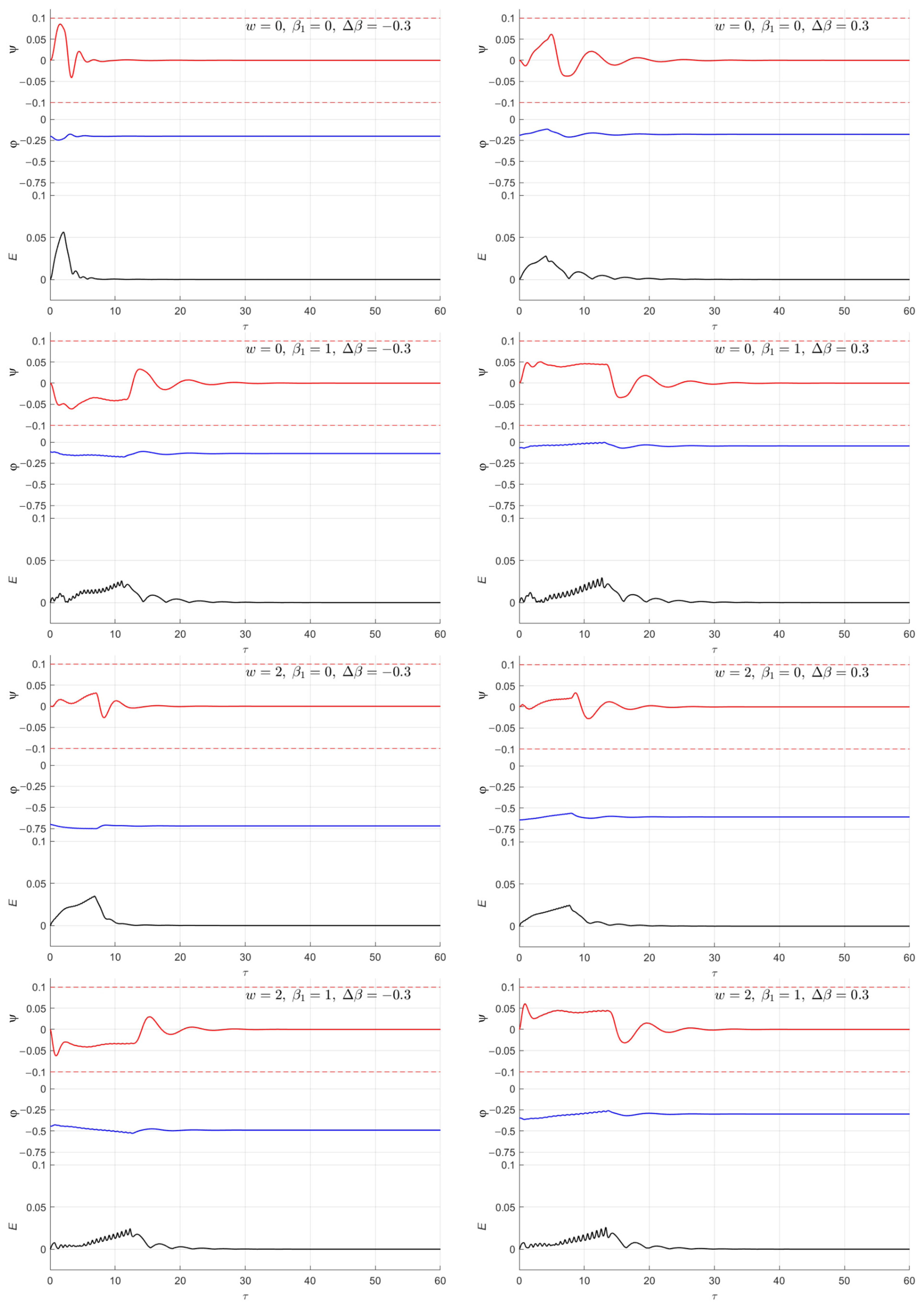
In Figure 7, results of the system dynamics numerical simulation are shown for different angles of inclination of the first and the second segments and for various wind speeds. The dependences of the following variables on the dimensionless time $\tau$ are presented here: angles $\psi$ (red lines) and $\phi$ (blue lines), as well as the error $E$ (black lines). The value E characterizes the deviation of position in the copter’s center of mass from the program trajectory, i.e.:

$$E=\sqrt{{\left(x-x^p\right)}^2+{\left(y-y^p\right)}^2}.$$

(41)

One can readily see that the proposed control ensures the transition from the first segment to the second one in such a way that the amplitude of oscillations of the fluid remains within the prescribed range (boundaries $\pm {\psi }_m$ of this range are shown in Figure 7 with dotted lines). It should be noted that the algorithm is efficient for relatively large values of $\Delta \beta$.

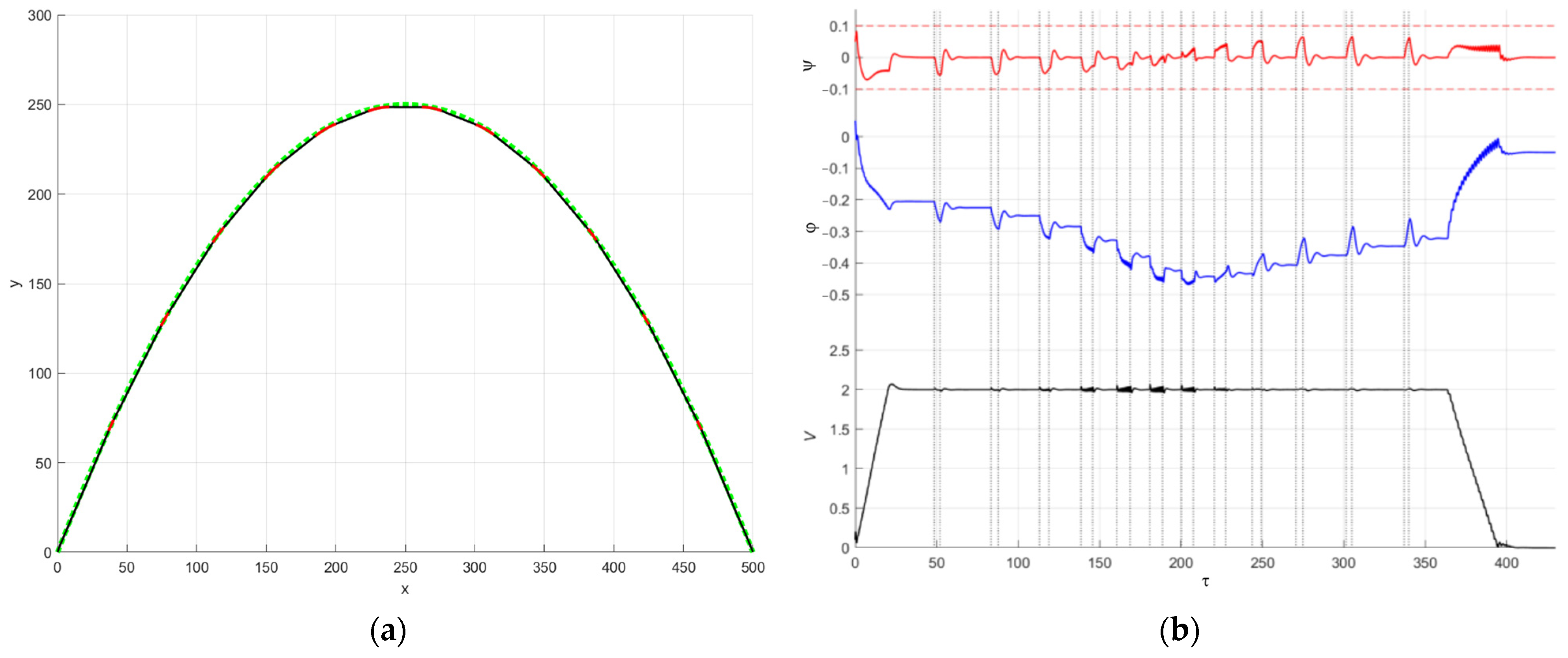
3.3. Numerical Simulation Example

As a numerical example illustrating the operation of the proposed algorithm, let us consider the following target motion: start and end positions are at the same altitude, the normalized distance between them is 500, and the center of mass of the copter must move along the parabolic curve connecting these points:

$$y={\displaystyle \frac{x(500-x)}{250}}.$$

(42)

Let the normalized wind speed be equal to 1.

In order to determine the number $N_s$ of segments, we restrict the difference between tangents of angles of inclination of neighbor segments with 0.3. Then, we obtain $N_s=13$, which means that the curve should be divided into 13 straight segments and 12 circular arcs connecting them.

The result of numerical simulation is shown in Figure 8. The target trajectory is shown in Figure 8a with green dots, and the calculated path of the copter center of mass is shown with black (for straight segments) and red lines (for curvilinear segments).

In Figure 8b, time dependences of angles $\psi$ (red line), $\phi$ (blue line), and $V$ (black line) are shown. Grey vertical lines denote the start/end moments of trajectory segments.

The calculated trajectory tracks approximate the target trajectory rather well. In order to make the difference smaller, one can just increase the number of segments. However, if the first and/or the last segment becomes shorter than $v_c^2/2\overline{a}$, the algorithm needs to be upgraded in order to allow for the acceleration/deceleration stage to comprise several neighbor segments.

The amplitude of oscillations of the pendulum characterizing the dynamics of the fluid does not exceed ${\psi }_m$; however, at the acceleration stages, this amplitude sometimes comes relatively close to this limitation.

Thus, the main objective of the control is achieved: the copter with the payload followed the target trajectory with the prescribed cruising speed, and the oscillations of the fluid in the container remained within the specified limits.

4. Conclusions

The proposed strategy for controlling a copter with a slung load partially filled with fluid ensures such motion of the copter center of mass along the prescribed smooth enough trajectory that the amplitude of oscillations of fluid inside the payload remains within the specified limits for wide enough range of values of the wind speed and inclination angles of segments. The control takes into account the aerodynamic drag force acting on the payload (including the presence of horizontal wind as well).

The angle between the neighbor rectilinear segments can differ considerably from the straight angle. The error (41) also remains small, which means that the target position of the copter is tracked well.

Note that increase in wind speed results in smaller oscillation amplitudes in the fluid.

A series of simulations of systems behavior was performed for different masses of fluid and different filling levels. Calculations showed that the control constructed according to the proposed method remains efficient. Simulations also show that the control is robust with respect to variation of initial conditions. Questions of robustness with respect to disturbances in parameters remain for future research.