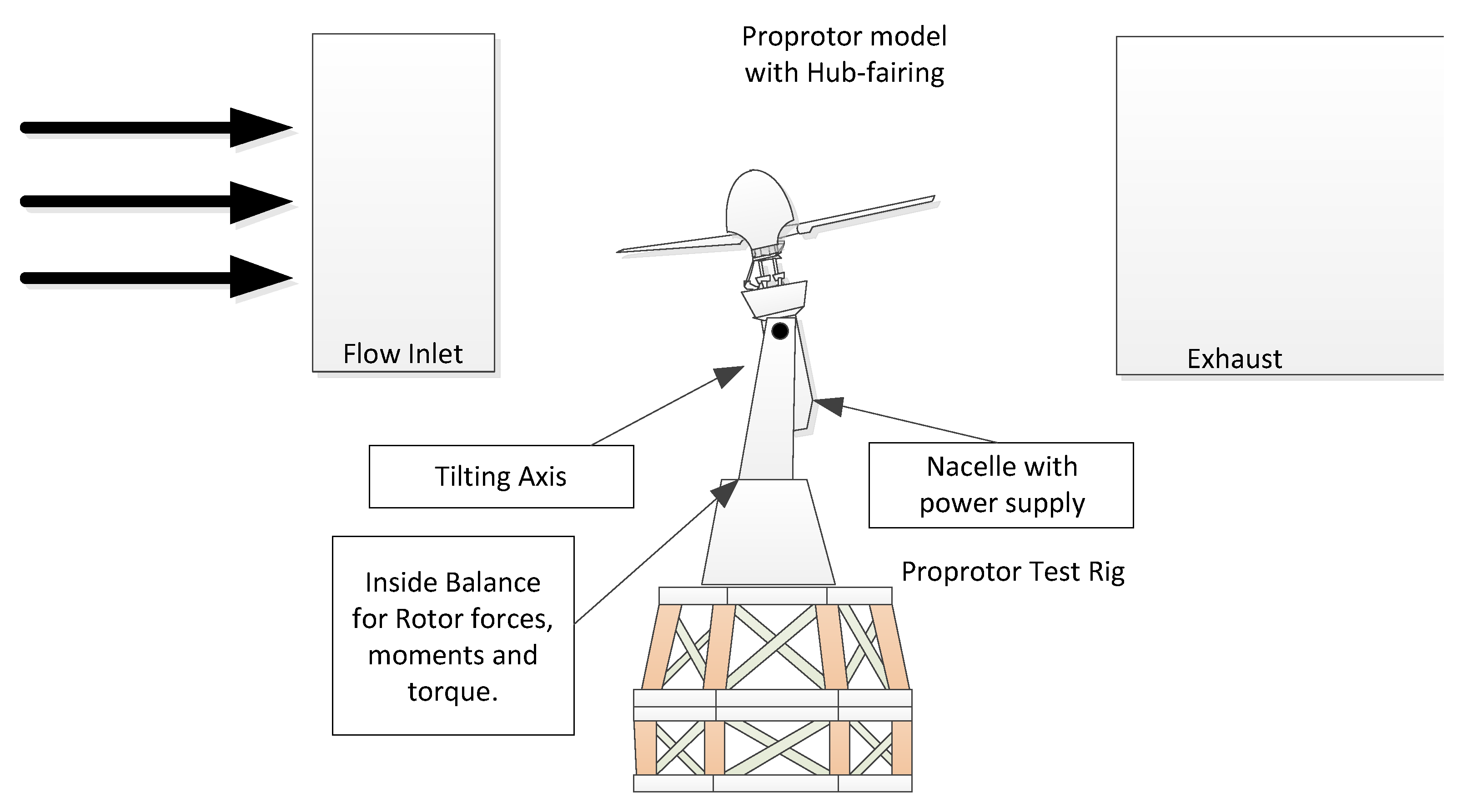
Figure 1.
Schematic of the wind tunnel test rig.
Figure 1.
Schematic of the wind tunnel test rig.
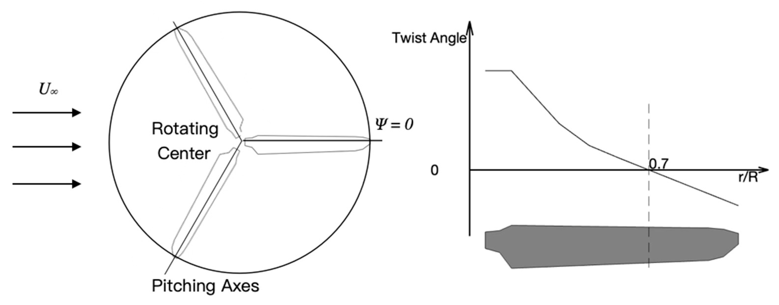
Figure 2.
Top view of the rotor disk and the blade geometry.
Figure 2.
Top view of the rotor disk and the blade geometry.
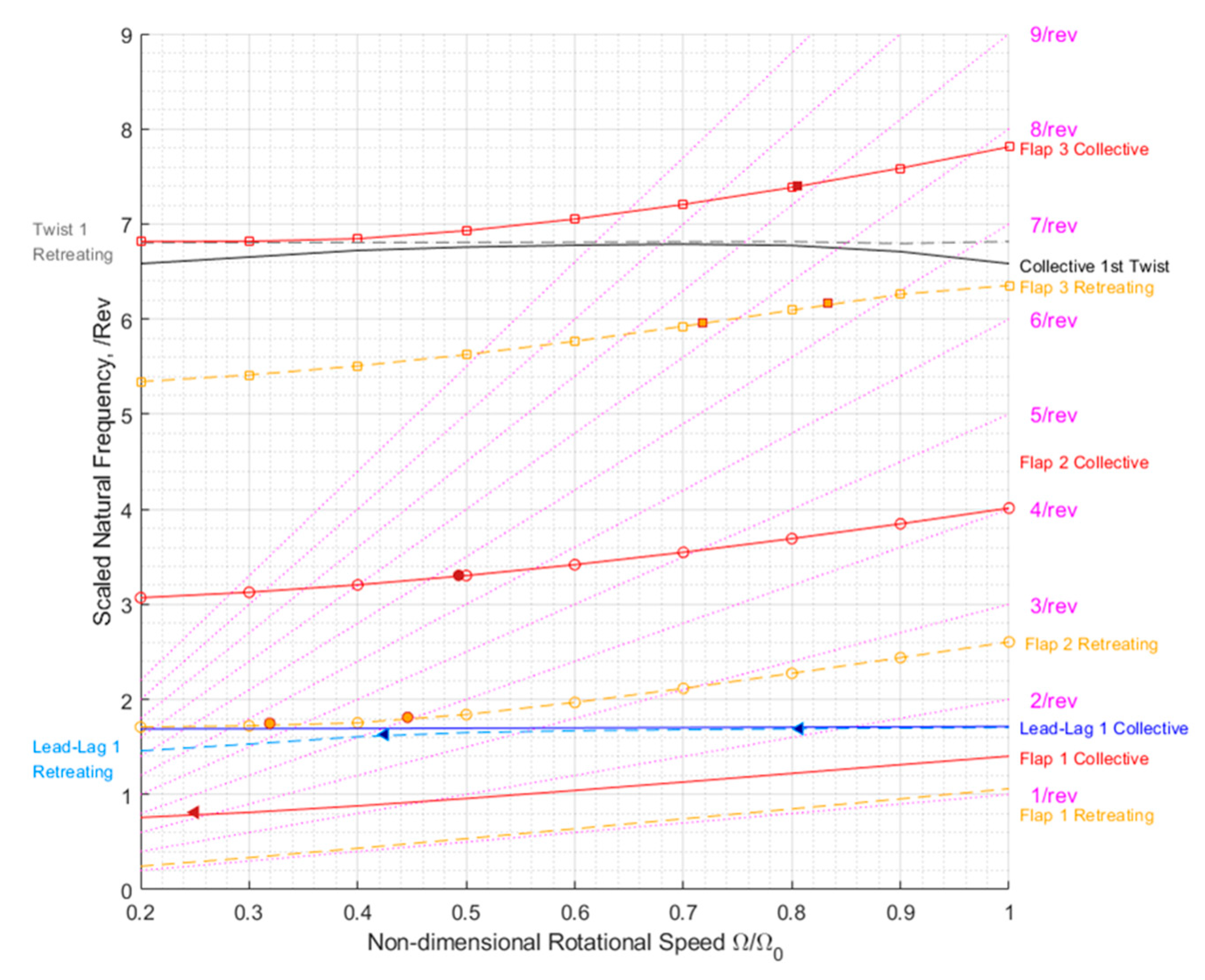
Figure 3.
Predicted and identified (filled markers) natural frequencies of blade modes.
Figure 3.
Predicted and identified (filled markers) natural frequencies of blade modes.
Figure 4.
Comparison of measured and simulated alternating bending moments with different aerodynamic models for helicopter mode. (a) Case 903 blade flap moments; (b) Case 903 blade lead-lag moments; (c) Case 802 blade flap moments; (d) Case 803 blade flap moments; (e) Case 803 blade flap moments; (f) Case 803 blade lead-lag moments; (g) Case 813 blade flap moments; (h) Case 813 lead-lag moments.
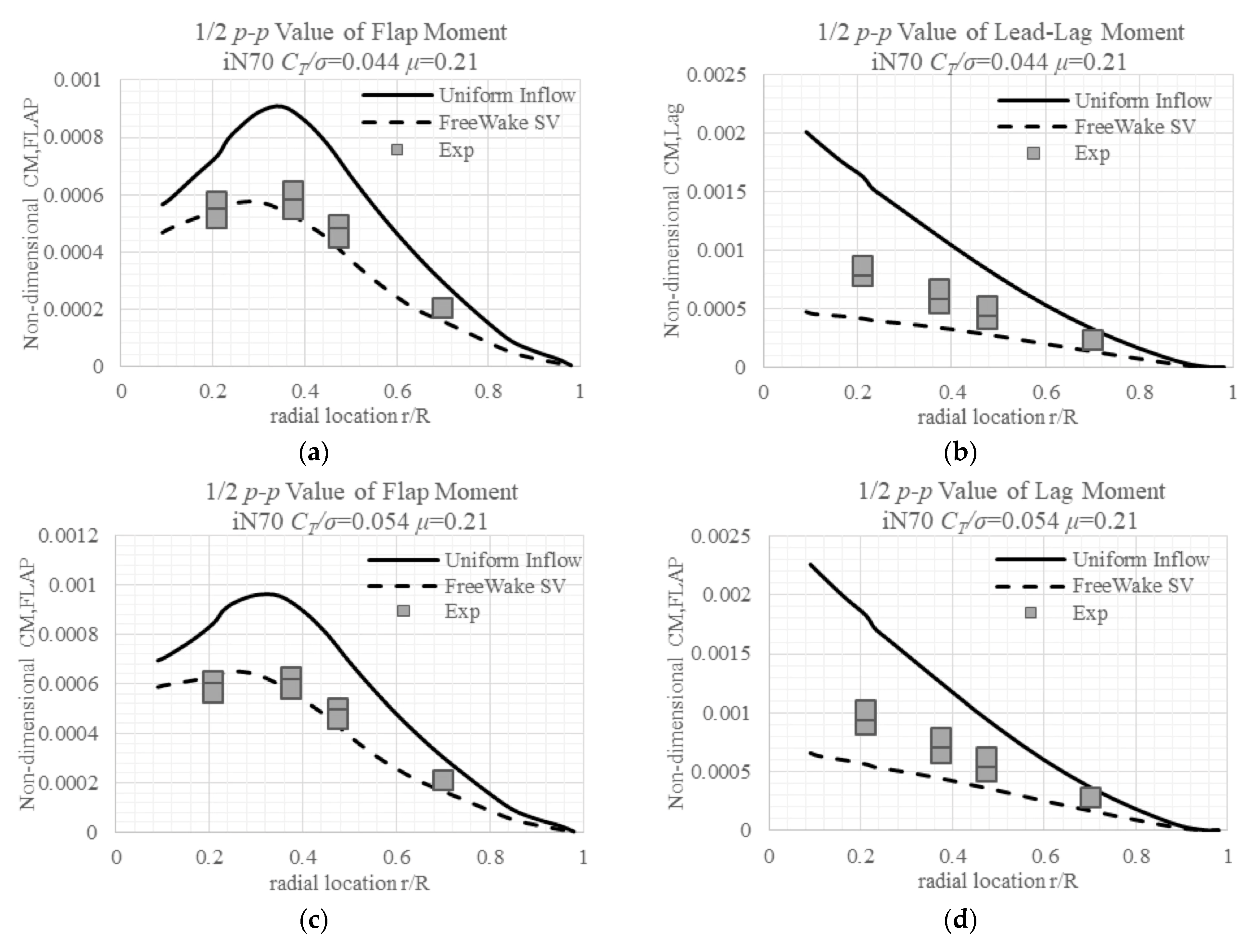
Figure 5.
Comparison of measured and simulated alternating bending moments with different inflow models for transition mode, nacelle angle 70°, and advance ratio 0.17. (a) Case 710 blade flap moments; (b) Case 710 blade lead-lag moments; (c) Case 711 blade flap moments; (d) Case 711 blade lead-lag moments; (e) Case 713 blade flap moments; (f) Case 713 lead-lag moments.
Figure 6.
Comparison of measured and simulated alternating bending moments with different inflow models for transition mode, nacelle angle 70°, and advance ratio 0.21~0.25. (a) Case 720 blade flap moments; (b) Case 720 blade lead-lag moments; (c) Case 721 blade flap moments; (d) Case 721 blade lead-lag moments; (e) Case 722 blade flap moments; (f) Case 722 blade lead-lag moments; (g) Case 740 blade flap moments; (h) Case 740 blade lead-lag moments.
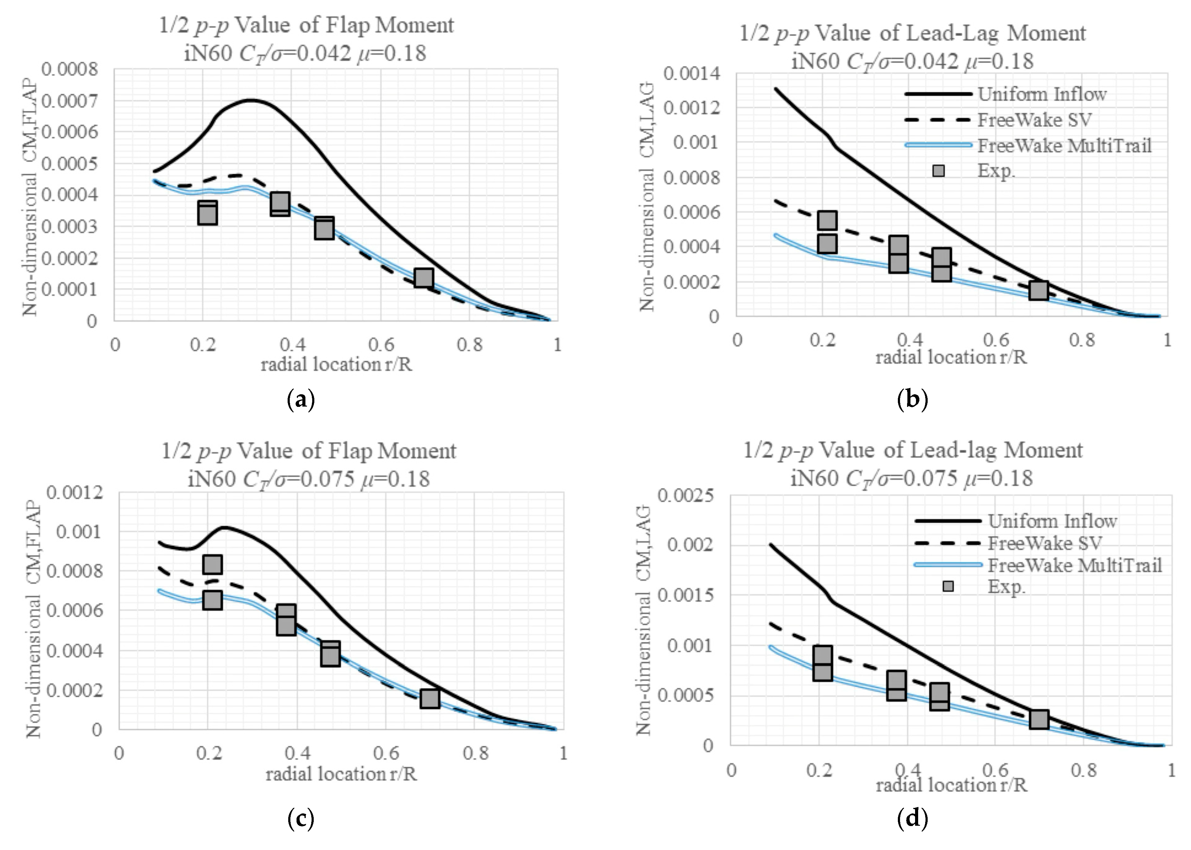
Figure 7.
Comparison of alternating bending moments with different inflow models for transition mode, nacelle angle 60°, and advance ratio 0.18~0.22. (a) Case 610 blade flap moments; (b) Case 610 blade lead-lag moments; (c) Case 612 blade flap moments; (d) Case 612 blade lead-lag moments; (e) Case 630 blade flap moments; (f) Case 630 blade lead-lag moments; (g) Case 632 blade flap moments; (h) Case 632 blade lead-lag moments.
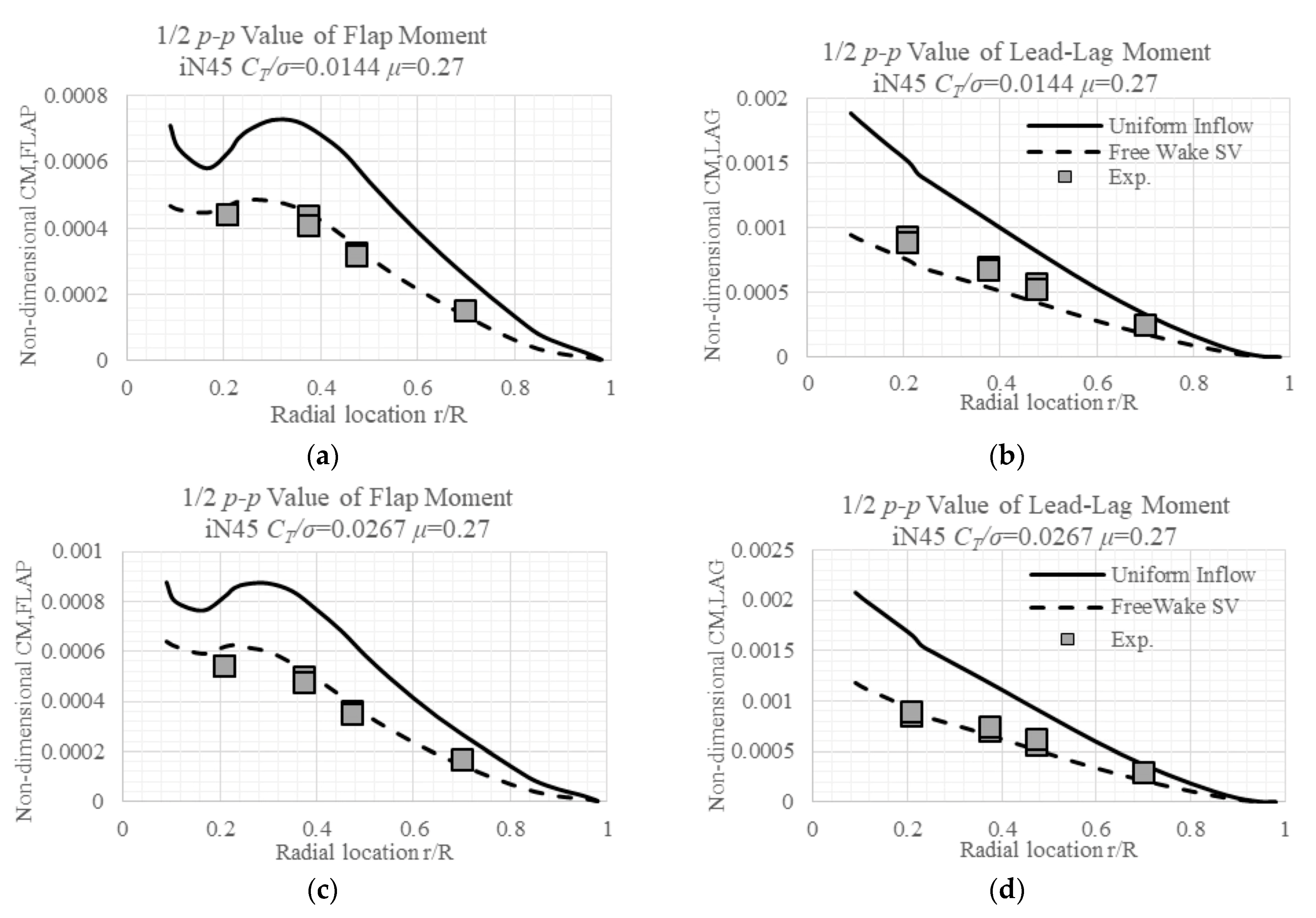
Figure 8.
Comparison of alternating bending moments with different inflow models for transition mode, nacelle angle 45°, advance ratio 0.27, and thrust coefficient 0.0144~0.0267. (a) Case 410 blade flap moments; (b) Case 410 blade lead-lag moments; (c) Case 411 blade flap moments; (d) Case 411 blade lead-lag moments.
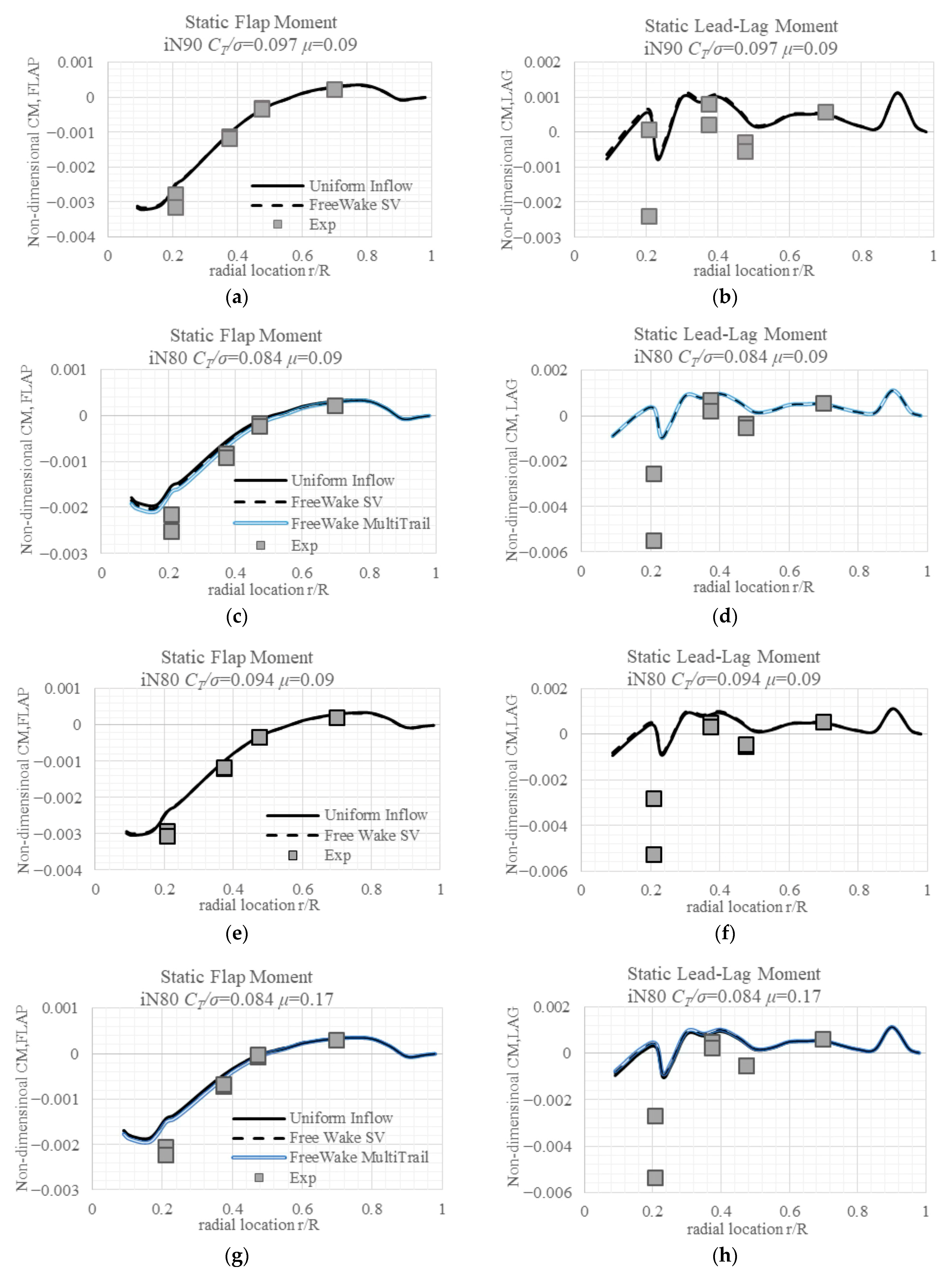
Figure 9.
Comparison of measured and simulated static bending moments with different aerodynamic models for helicopter mode. (a) Case 903 blade flap moments; (b) Case 903 blade lead-lag moments; (c) Case 802 blade flap moments; (d) Case 803 blade flap moments; (e) Case 803 blade flap moments; (f) Case 803 blade lead-lag moments; (g) Case 813 blade flap moments; (h) Case 813 lead-lag moments.
Figure 10.
Comparison of measured and simulated static bending moments with different inflow models for the transition mode, nacelle angle 70°, and advance ratio 0.17. (a) Case 710 blade flap moments; (b) Case 710 blade lead-lag moments; (c) Case 711 blade flap moments; (d) Case 711 blade lead-lag moments; (e) Case 713 blade flap moments; (f) Case 713 lead-lag moments.
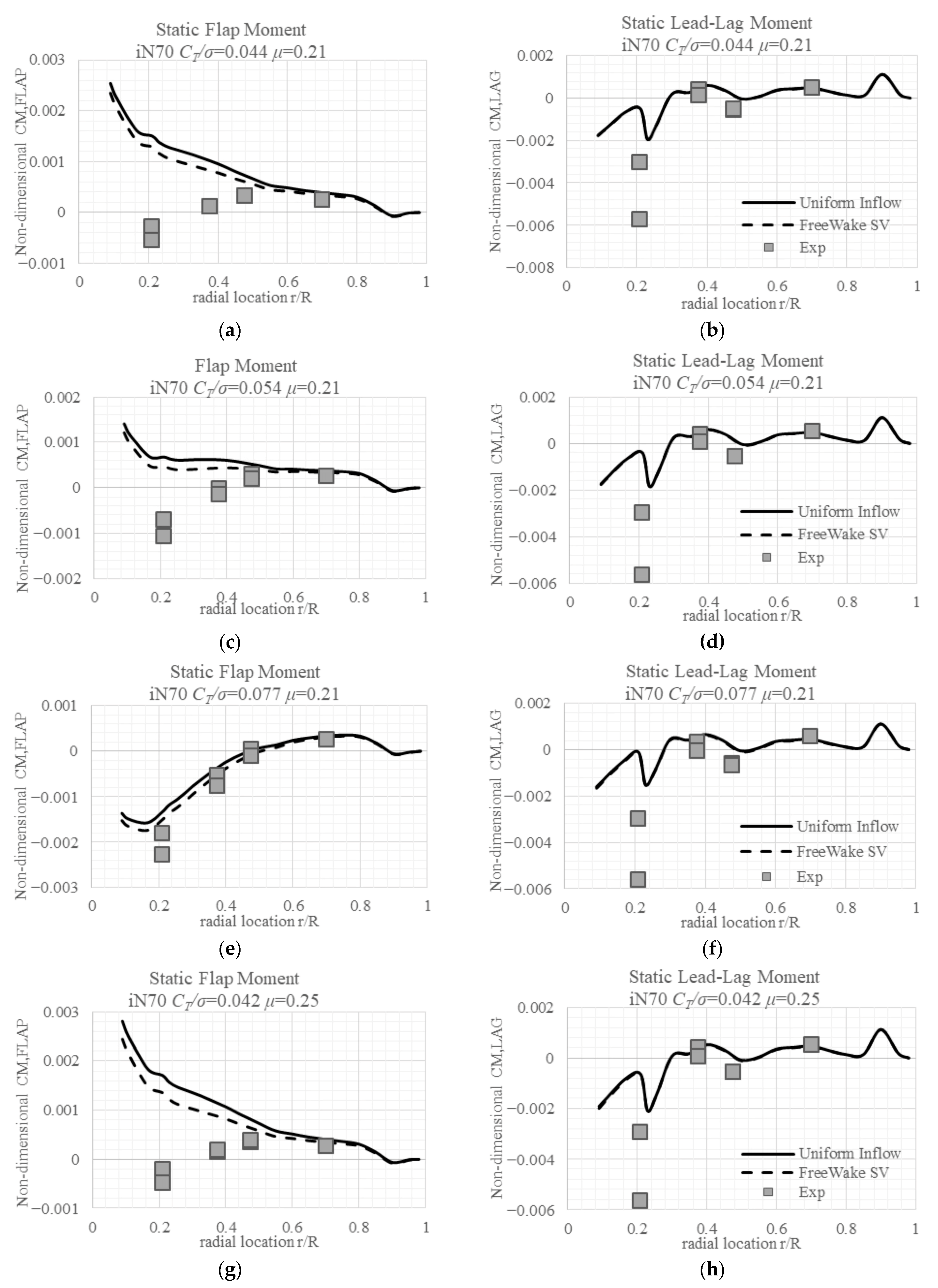
Figure 11.
Comparison of measured and simulated static bending moments with different inflow models for the transition mode, nacelle angle 70°, and advance ratio 0.21~0.25. (a) Case 720 blade flap moments; (b) Case 720 blade lead-lag moments; (c) Case 721 blade flap moments; (d) Case 721 blade lead-lag moments; (e) Case 722 blade flap moments; (f) Case 722 blade lead-lag moments; (g) Case 740 blade flap moments; (h) Case 740 blade lead-lag moments.
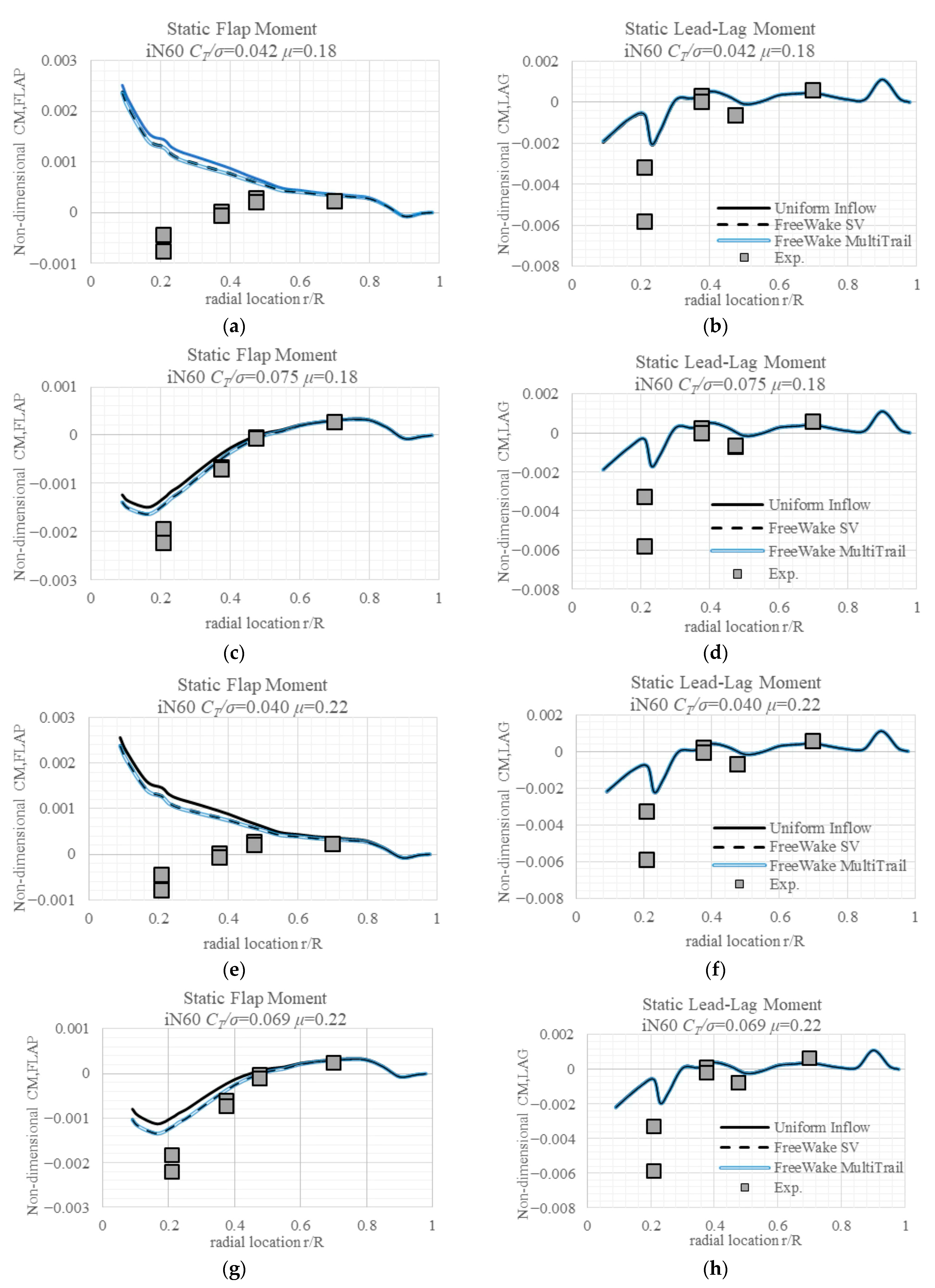
Figure 12.
Comparison of static bending moments with different inflow models for the transition mode, nacelle angle 60°, and advance ratio 0.18~0.22. (a) Case 610 blade flap moments; (b) Case 610 blade lead-lag moments; (c) Case 612 blade flap moments; (d) Case 612 blade lead-lag moments; (e) Case 630 blade flap moments; (f) Case 630 blade lead-lag moments; (g) Case 632 blade flap moments; (h) Case 632 blade lead-lag moments.
Figure 13.
Comparison of static bending moments with different inflow models for transition mode, nacelle angle 45°, advance ratio 0.27, and thrust coefficient 0.0144~0.0267. (a) Case 410 blade flap moments; (b) Case 410 blade lead-lag moments; (c) Case 411 blade flap moments; (d) Case 411 blade lead-lag moments.
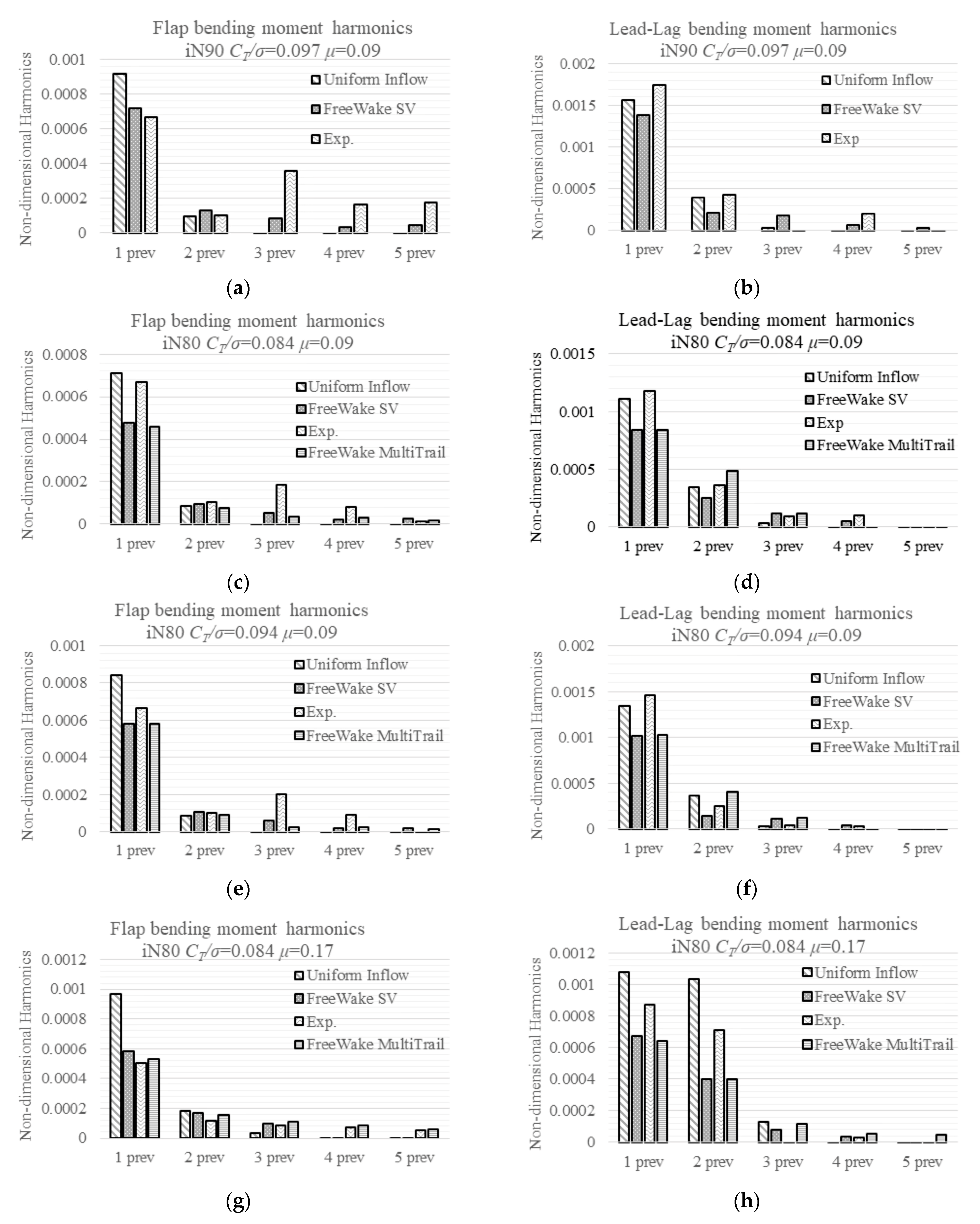
Figure 14.
Comparison of measured and simulated bending moments’ harmonics with different aerodynamic models for helicopter mode. (a) Case 903 blade flap moments’ harmonics; (b) Case 903 blade lead-lag moments’ harmonics; (c) Case 802 blade flap moments’ harmonics; (d) Case 803 blade flap moments’ harmonics; (e) Case 803 blade flap moments’ harmonics; (f) Case 803 blade lead-lag moments’ harmonics; (g) Case 813 blade flap moments’ harmonics; (h) Case 813 lead-lag moments’ harmonics.
Figure 15.
Comparison of measured and simulated bending moments’ harmonics with different inflow models for the transition mode, nacelle angle 70°, and advance ratio 0.17. (a) Case 710 blade flap moments’ harmonics; (b) Case 710 blade lead-lag moments’ harmonics; (c) Case 711 blade flap moments’ harmonics; (d) Case 711 blade lead-lag moments’ harmonics; (e) Case 713 blade flap moments’ harmonics; (f) Case 713 lead-lag moments’ harmonics.
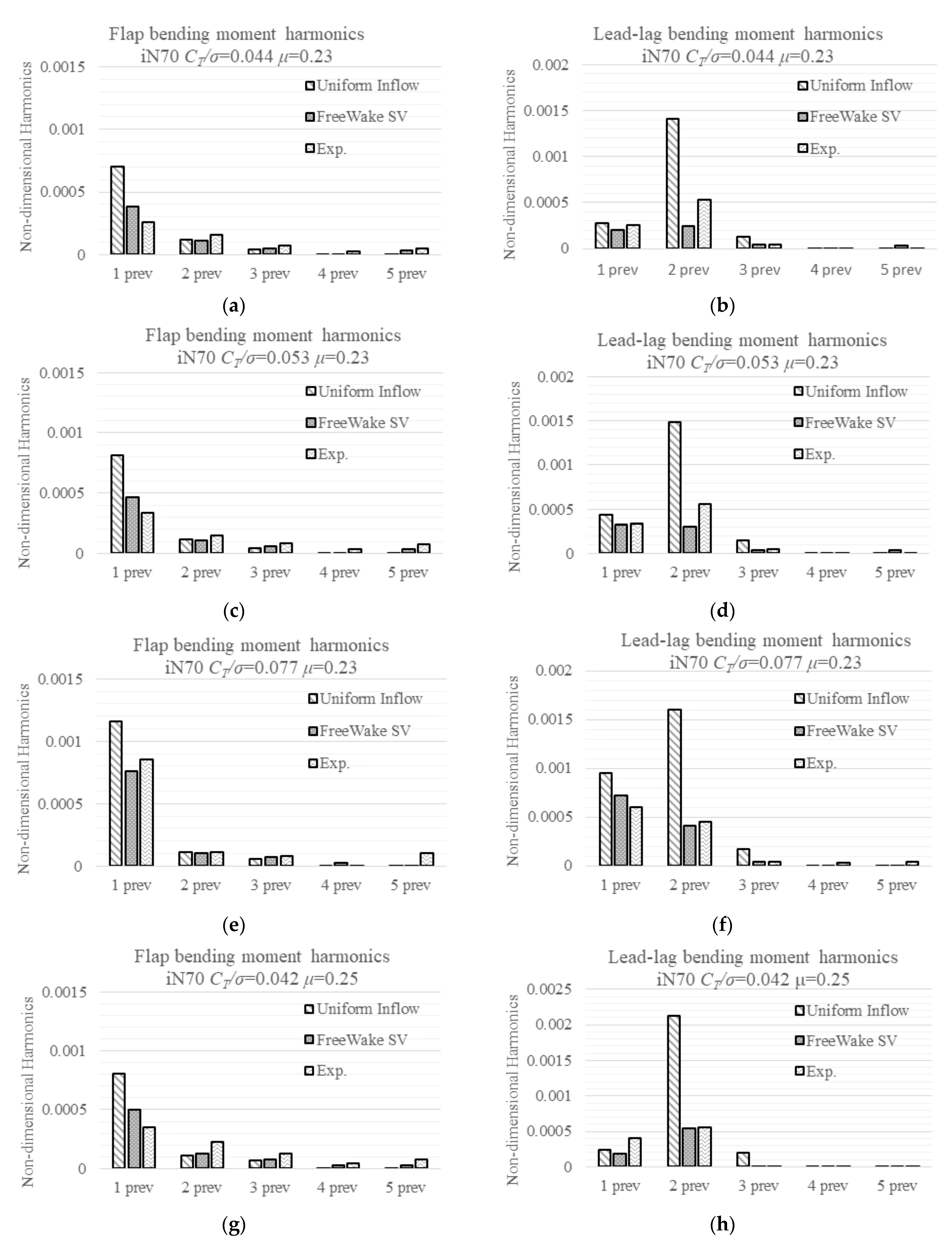
Figure 16.
Comparison of measured and simulated bending moments’ harmonics with different inflow models for the transition mode, nacelle angle 70°, and advance ratio 0.23~0.25. (a) Case 720 blade flap moments’ harmonics; (b) Case 720 blade lead-lag moments’ harmonics; (c) Case 721 blade flap moments’ harmonics; (d) Case 721 blade lead-lag moments’ harmonics; (e) Case 722 blade flap moments’ harmonics; (f) Case 722 blade lead-lag moments’ harmonics; (g) Case 740 blade flap moments’ harmonics; (h) Case 740 blade lead-lag moments’ harmonics.
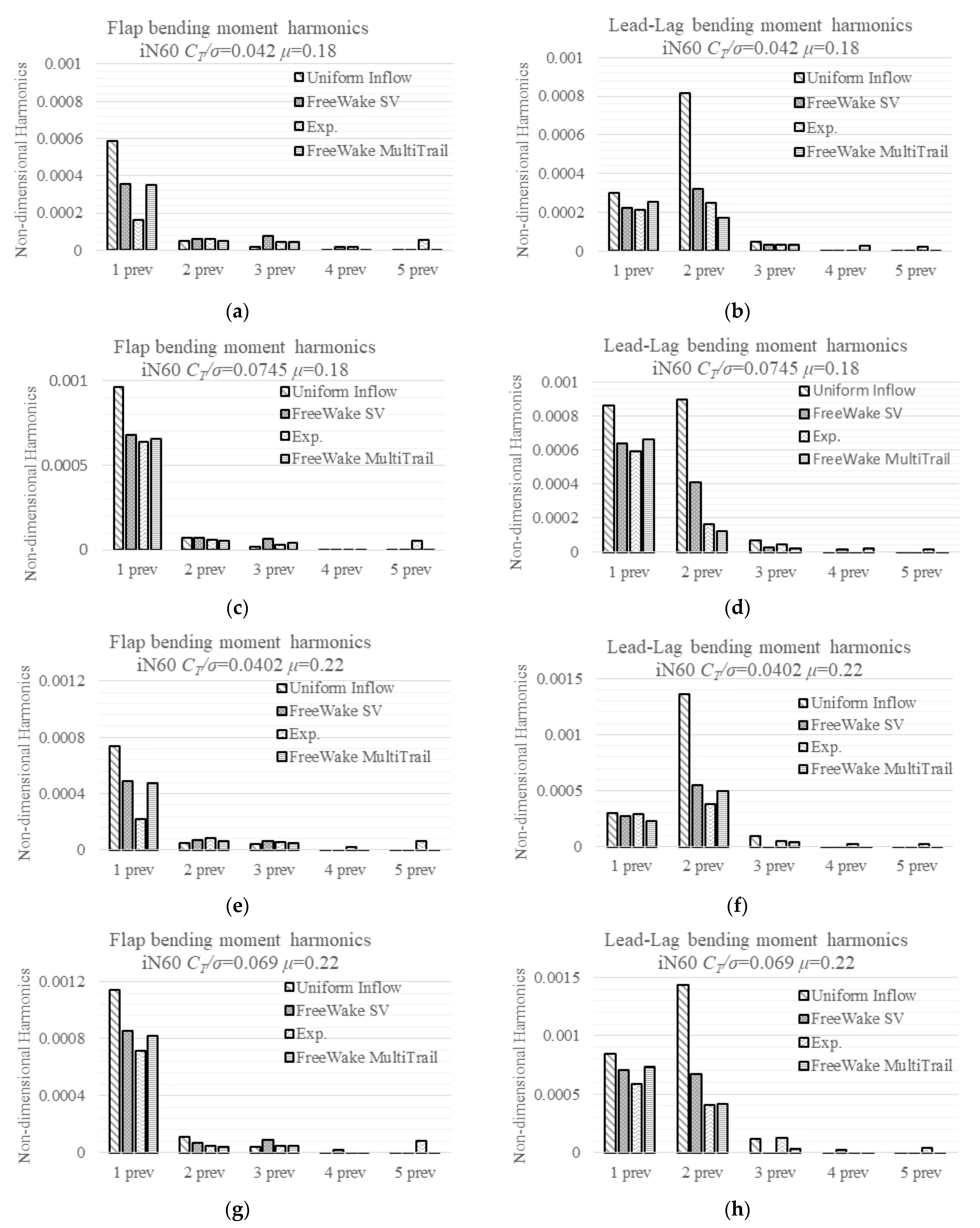
Figure 17.
Comparison of measured and simulated bending moments’ harmonics with different inflow models for the transition mode, nacelle angle 60°, and advance ratio 0.18~0.22. (a) Case 610 blade flap moments’ harmonics; (b) Case 610 blade lead-lag moments’ harmonics; (c) Case 612 blade flap moments’ harmonics; (d) Case 612 blade lead-lag moments’ harmonics; (e) Case 630 blade flap moments’ harmonics; (f) Case 630 blade lead-lag moments’ harmonics; (g) Case 632 blade flap moments’ harmonics; (h) Case 632 blade lead-lag moments’ harmonics.
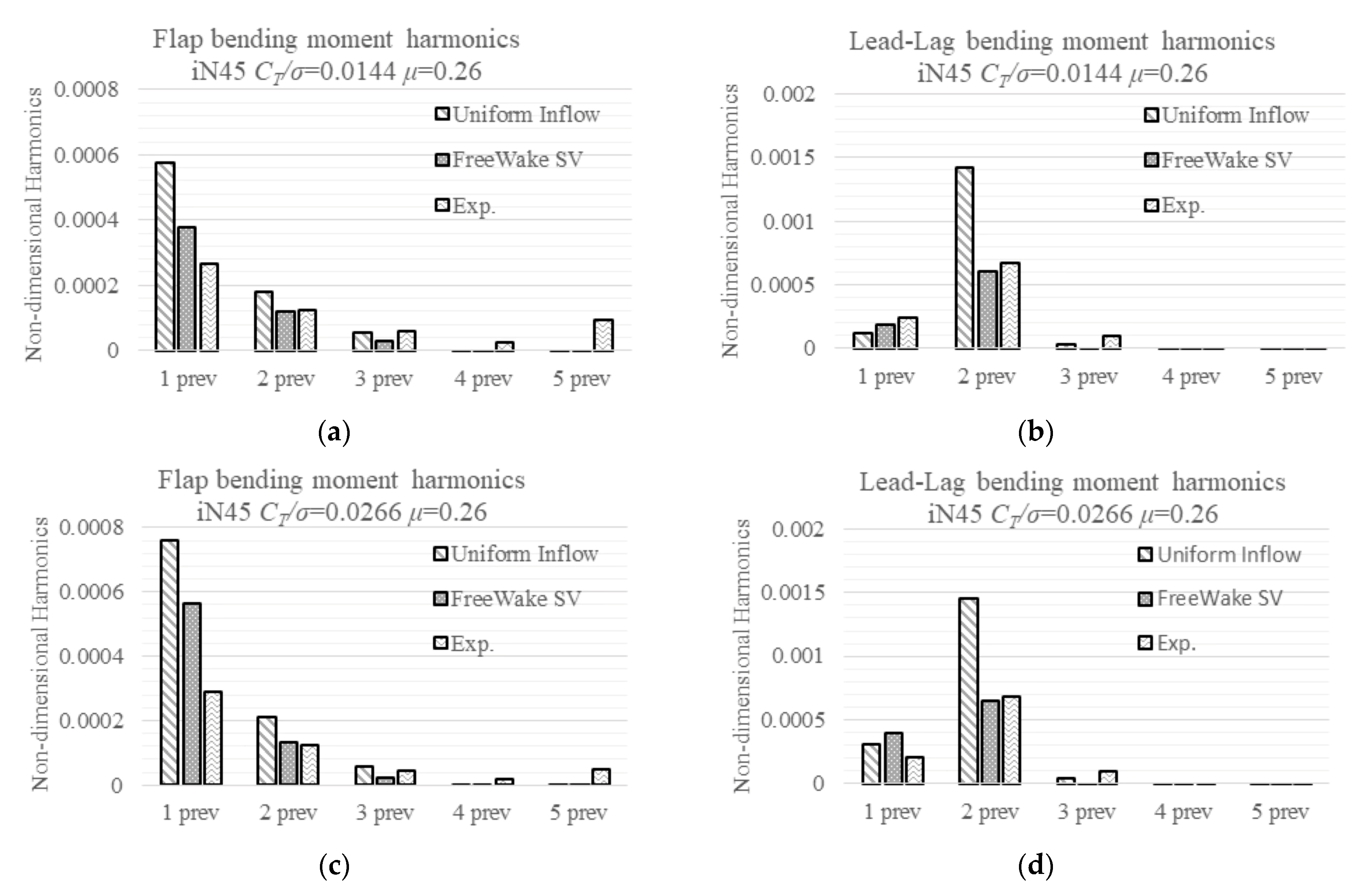
Figure 18.
Comparison of measured and simulated bending moments’ harmonics with different inflow models for the transition mode, nacelle angle 45°, advance ratio 0.26, and CT/σ = 0.0144~0.0266. (a) Case 410 blade flap moments’ harmonics; (b) Case 410 blade lead-lag moments’ harmonics’ harmonics; (c) Case 411 blade flap moments’ harmonics; (d) Case 411 blade lead-lag moments’ harmonics.
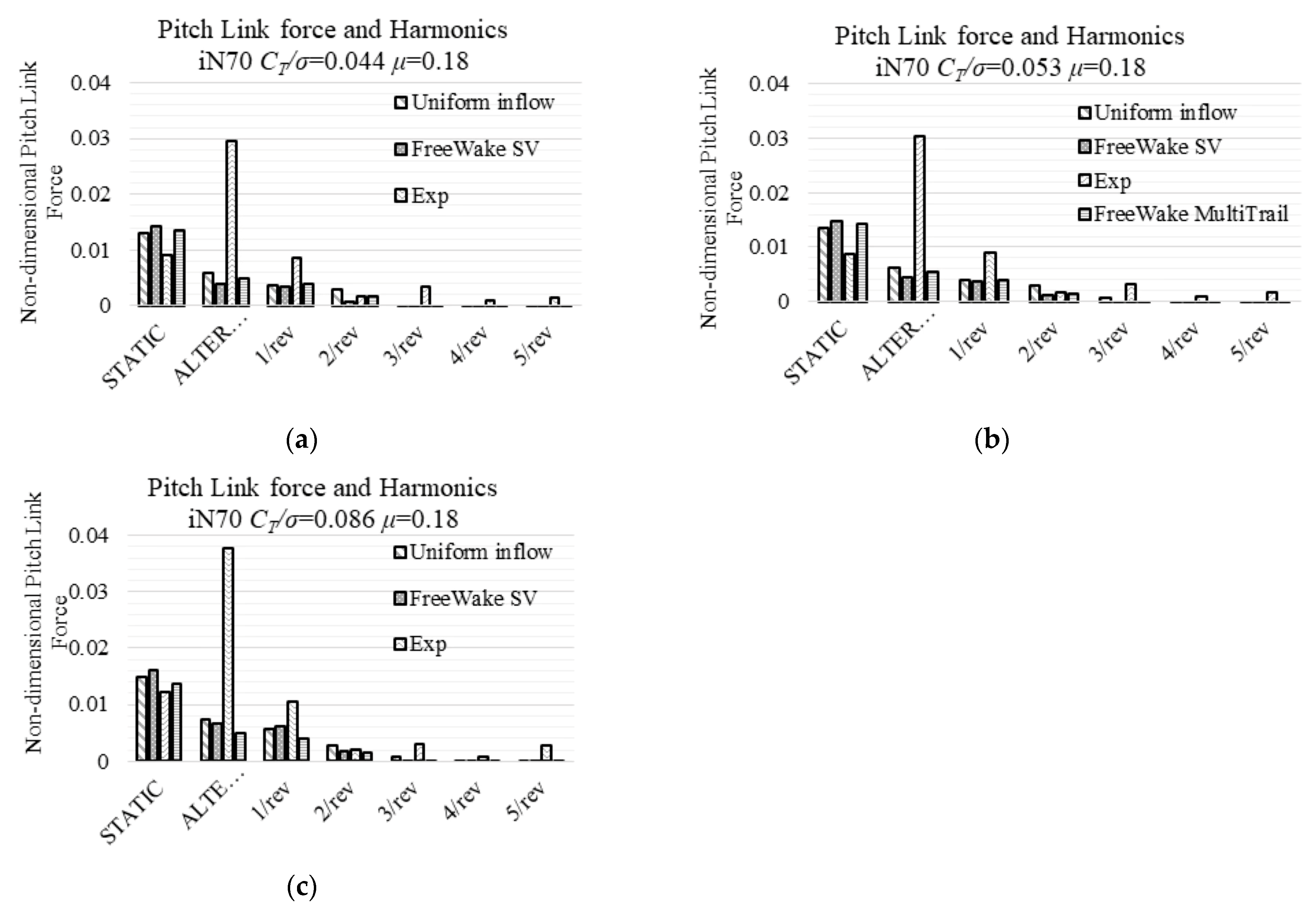
Figure 19.
Comparison of measured and simulated pitch link force (static and alternating loads, and harmonics) with different inflow models for helicopter mode. (a) Case 903 pitch link force; (b) Case 802 pitch link force; (c) Case 803 pitch link force; (d) Case 812 pitch link force.
Figure 19.
Comparison of measured and simulated pitch link force (static and alternating loads, and harmonics) with different inflow models for helicopter mode. (a) Case 903 pitch link force; (b) Case 802 pitch link force; (c) Case 803 pitch link force; (d) Case 812 pitch link force.
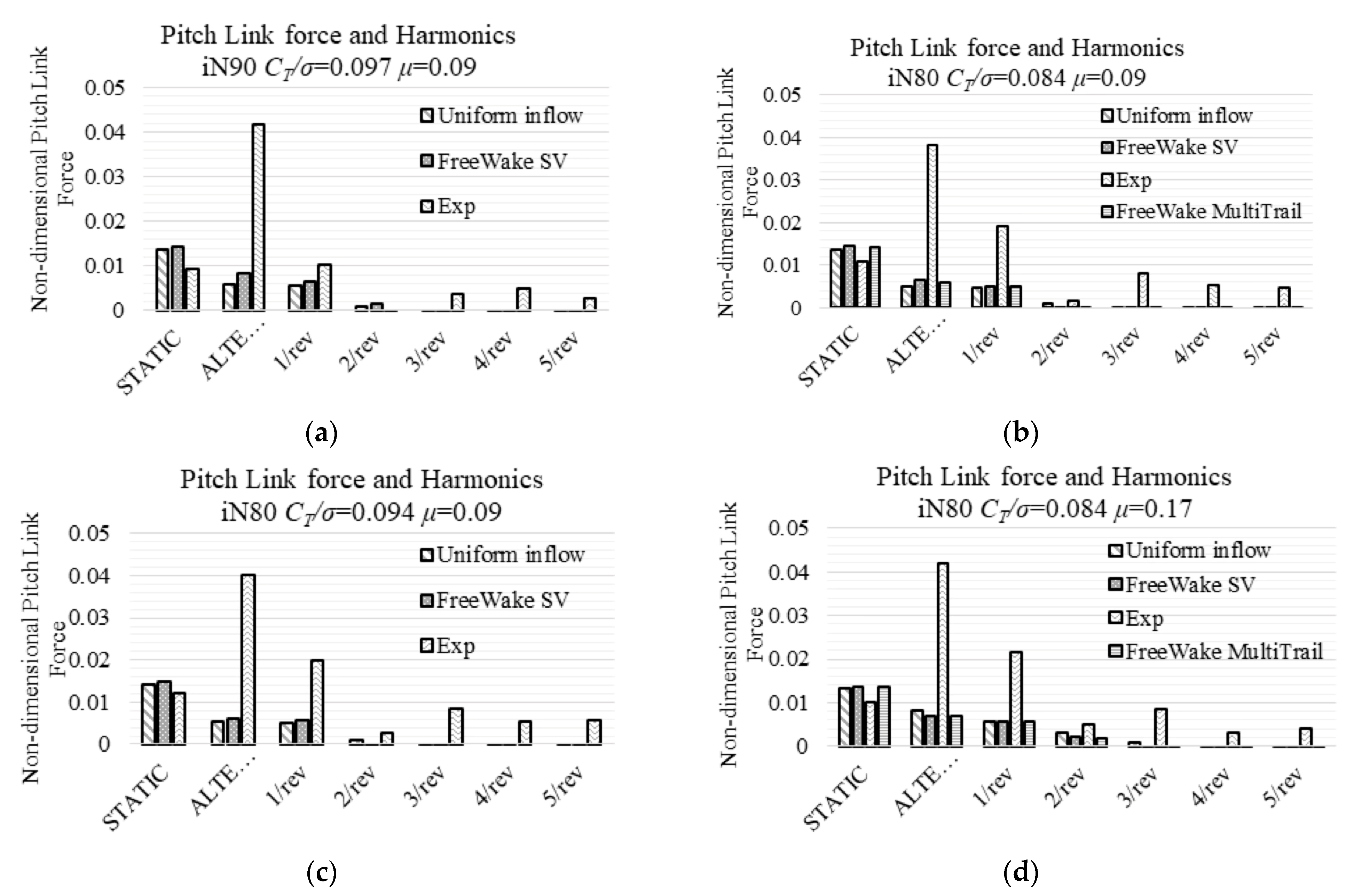
Figure 20.
Comparison of measured and simulated pitch link force (including harmonics) with different inflow models for the transition mode, nacelle angle 70°, and advance ratio 0.18. (a) Case 710 pitch link force; (b) Case 711 pitch link force; (c) Case 713 pitch link forces.
Figure 20.
Comparison of measured and simulated pitch link force (including harmonics) with different inflow models for the transition mode, nacelle angle 70°, and advance ratio 0.18. (a) Case 710 pitch link force; (b) Case 711 pitch link force; (c) Case 713 pitch link forces.
Figure 21.
Comparison of measured and simulated pitch link force (including harmonics) with different inflow models for the transition mode, nacelle angle 70°, and advance ratio 0.23~0.25. (a) Case 720 pitch link force; (b) Case 721 pitch link force; (c) Case 722 pitch link force; (d) Case 740 pitch link force.
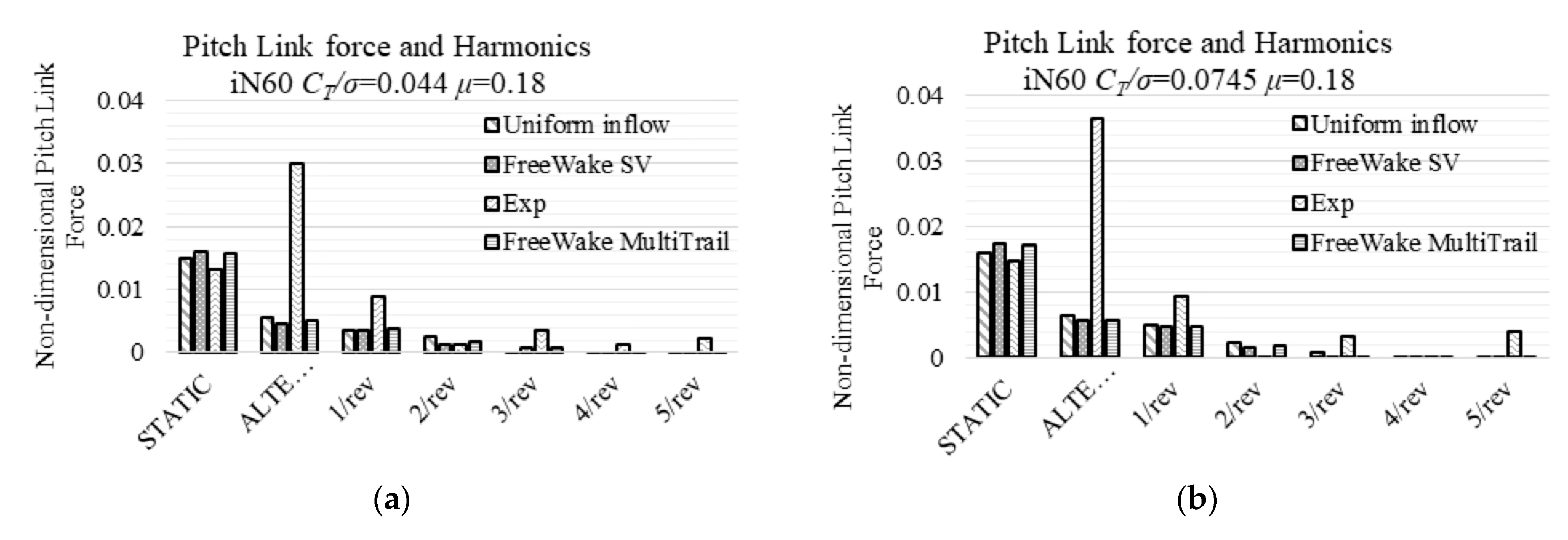
Figure 22.
Comparison of measured and simulated pitch link force (including harmonics) with different inflow models for the transition mode, nacelle angle 60°, and advance ratio 0.18~0.22. (a) Case 610 pitch link force; (b) Case 612 pitch link force; (c) Case 630 pitch link force; (d) Case 632 pitch link force.
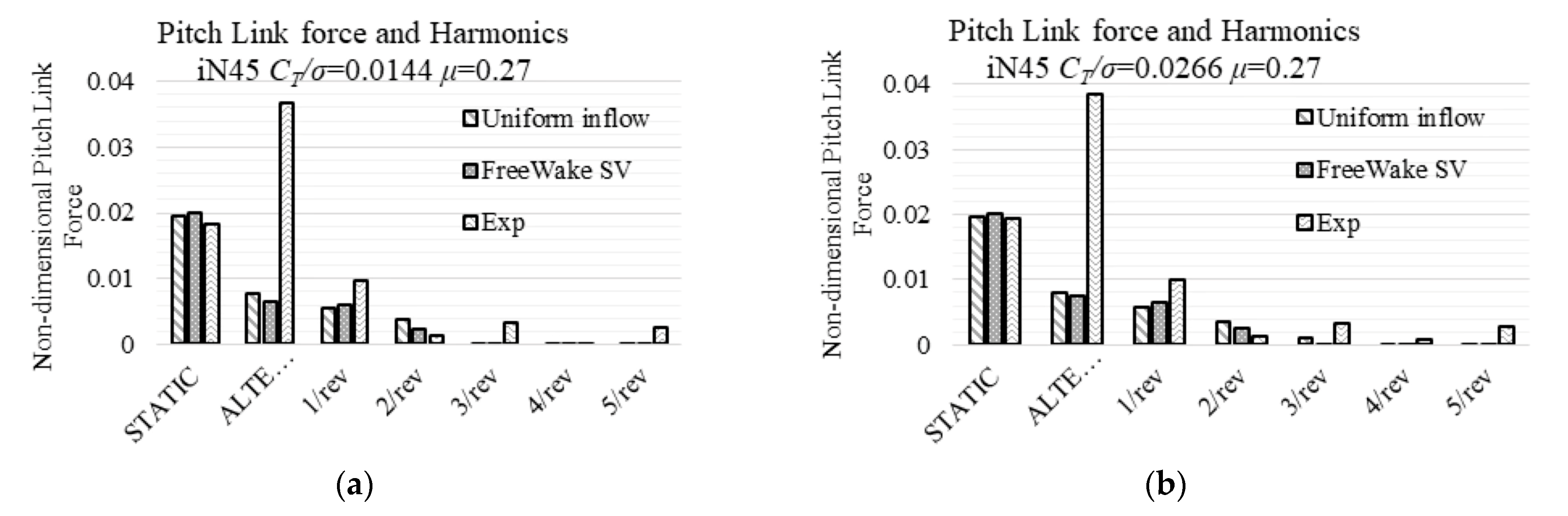
Figure 23.
Comparison of measured and simulated pitch link force (including harmonics) with different inflow models for the transition mode, nacelle angle 45°, and advance ratio 0.27. (a) Case 410 pitch link force; (b) Case 411 pitch link force.
Figure 23.
Comparison of measured and simulated pitch link force (including harmonics) with different inflow models for the transition mode, nacelle angle 45°, and advance ratio 0.27. (a) Case 410 pitch link force; (b) Case 411 pitch link force.
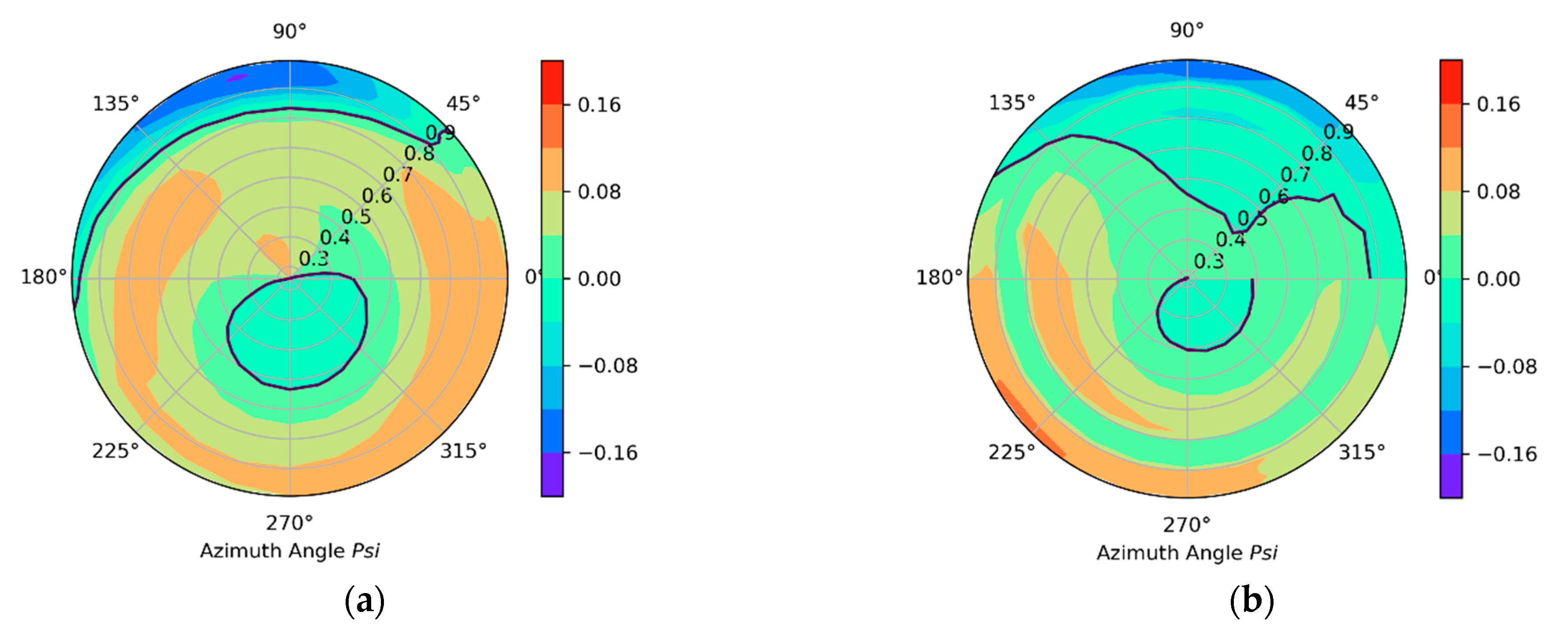
Figure 24.
Comparison of CmM2 predicted by (a) the RCAC Linear inflow model and (b) CFD with a rigid blade assumption for case iN45, μ = 0.27, CT/σ = 0.0266.
Figure 24.
Comparison of CmM2 predicted by (a) the RCAC Linear inflow model and (b) CFD with a rigid blade assumption for case iN45, μ = 0.27, CT/σ = 0.0266.
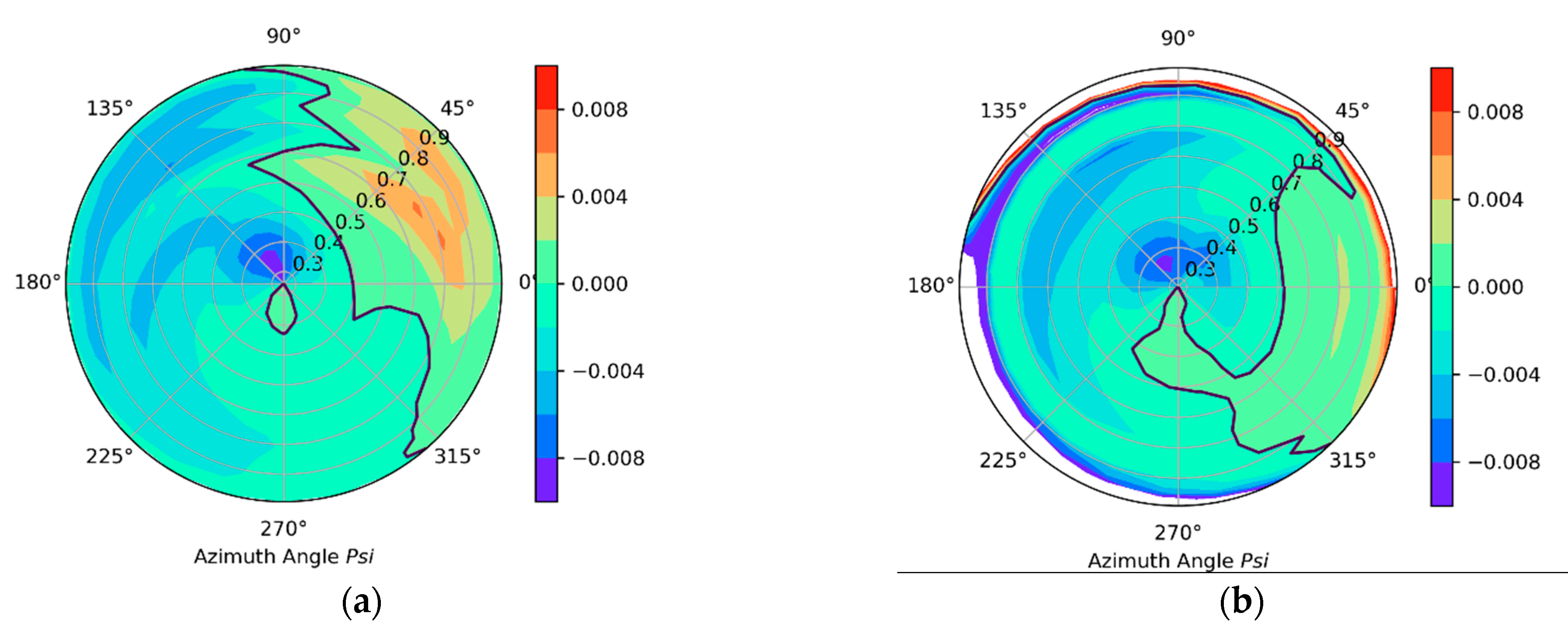
Figure 25.
Comparison of CnM2 predicted by (a) the RCAC Linear inflow model and (b) CFD with a rigid blade assumption for case iN45, μ = 0.27, CT/σ = 0.0266.
Figure 25.
Comparison of CnM2 predicted by (a) the RCAC Linear inflow model and (b) CFD with a rigid blade assumption for case iN45, μ = 0.27, CT/σ = 0.0266.
Table 1.
Operating conditions of the model tilt-proprotor in the CHRDI wind tunnel.
Table 1.
Operating conditions of the model tilt-proprotor in the CHRDI wind tunnel.
| Case Index | Mode | Rotor mast Angle, ° | Advance Ratio, μ | Thrust Coefficient
CT/σ |
|---|
| 903 | Heli | 90 | 0.09 | 0.097 |
| 802 | Heli | 80 | 0.09 | 0.084 |
| 803 | Heli | 80 | 0.09 | 0.094 |
| 812 | Heli | 80 | 0.17 | 0.084 |
| 710 | Conv | 70 | 0.17 | 0.044 |
| 711 | Conv | 70 | 0.17 | 0.053 |
| 713 | Conv | 70 | 0.17 | 0.087 |
| 720 | Conv | 70 | 0.21 | 0.044 |
| 721 | Conv | 70 | 0.21 | 0.054 |
| 722 | Conv | 70 | 0.21 | 0.077 |
| 740 | Conv | 70 | 0.25 | 0.042 |
| 610 | Conv | 60 | 0.18 | 0.042 |
| 612 | Conv | 60 | 0.18 | 0.075 |
| 630 | Conv | 60 | 0.23 | 0.040 |
| 632 | Conv | 60 | 0.23 | 0.069 |
| 410 | Conv | 45 | 0.19 | 0.0144 |
| 411 | Conv | 45 | 0.19 | 0.0266 |
Table 2.
RSD values for the alternating structural moments.
Table 2.
RSD values for the alternating structural moments.
| r/R | Flap Moments, Blade 1 | Flap Moments, Blade 2 | Lead-Lag Moments, Blade 1 | Lead-Lag Moments, Blade 2 |
|---|
| 0.21 | 1.6373% | 0.9893% | 4.3250% | 2.5204% |
| 0.375 | 0.6676% | 0.5861% | 3.5428% | 3.5721% |
| 0.475 | 0.4507% | 0.6226% | 3.4147% | 3.1005% |
| 0.7 | | 0.2098% | | 2.1291% |
Table 3.
Model predicted vs. measured structural loads: difference and blade-to-blade variation, iN90-iN80.
Table 3.
Model predicted vs. measured structural loads: difference and blade-to-blade variation, iN90-iN80.
| Case | Radial Location r/R | Linear Inflow Model | Free Wake Single Vortex Model | Free Wake Multi-Trailed Model |
|---|
| Flap Moment Difference and Blade–Blade Variation
| Lead-Lag Moment Difference and Blade–Blade Variation
| Flap Moment Difference and Blade–Blade Variation
| Lead-Lag Moment Difference and Blade–Blade Variation
| Flap Moment Difference and Blade–Blade Variation
| Lead-Lag Moment Difference and Blade–Blade Variation
|
|---|
| 903 | 0.21 | −22 (5.6) | −24.7 (3.3) | −34.7 (4.7) | −24 (3.3) | | |
| 0.375 | 0.1 (1.9) | −32.4 (0.6) | −21 (0) | −31 (0.6) | | |
| 0.475 | 6.7 (1.7) | −35 (1.0) | −21 (8.9) | −32.4 (1.0) | | |
| 0.7 | −50 | −40.4 | −33 | −36 | | |
| 802 | 0.21 | −8.4 (5.5) | −6.5 (4.1) | −38 (3.8) | −22 (3.4) | −23.6 (4.6) | −21 (3.5) |
| 0.375 | +22.5 (2.6) | −16 (1.7) | −13.2 (1.8) | −28 (2.5) | −11 (1.9) | −24.5 (1.6) |
| 0.475 | +42 (4.0) | −21.4 (0.2) | −6.3 (3) | −30 (0.3) | −12 (3.2) | −27 (0.3) |
| 0.7 | −34.5 | −32 | −27.2 | −35 | −22 | −33.5 |
| 803 | 0.21 | −17.4 (0.5) | −6.8 (0.5) | −30.8 (0.4) | −25.5 (0.4) | | |
| 0.375 | +26.4 (0.8) | −15.6 (1.0) | −11.7 (0.6) | −30.4 (3.5) | | |
| 0.475 | +47.8 (0.1) | −19.4 (1.0) | +8.6 (0.1) | −28.8 (0.8) | | |
| 0.7 | −40.2 | −33 | −37.4 | −36 | | |
| 812 | 0.21 | +21.7 (2.8) | +25.8 (2) | −16.1 (1.9) | −40.6 (0.9) | −18.3 (1.9) | −39.1 (0.9) |
| 0.375 | +38.5 (4.8) | +14.2 (5.5) | −2.0 (3.4) | −43.2 (3.7) | −13.2 (3) | −40.1 (2.9) |
| 0.475 | +39.6 (4.6) | +9.8 (6) | −4.6 (3.2) | −46.2 (2.9) | −5 (3.2) | −39.5 (3.3) |
| 0.7 | +11.8 | −2.7 | −36.8 | −39.9 | −9.6 | −35.7 |
Table 4.
Model predicted vs. measured structural loads: difference and blade-to-blade variation iN70-1.
Table 4.
Model predicted vs. measured structural loads: difference and blade-to-blade variation iN70-1.
| Case | Radial Location r/R | Linear Inflow Model | Free Wake Single Vortex Model | Free Wake Multi-Trailed Model |
|---|
| Flap Moment Difference and Blade–Blade Variation
| Lead-Lag Moment Difference and Blade–Blade Variation
| Flap Moment Difference and Blade–Blade Variation
| Lead-Lag Moment Difference and Blade–Blade Variation
| Flap Moment Difference and Blade–Blade Variation
| Lead-Lag Moment Difference and Blade–Blade Variation
|
|---|
| 710 | 0.21 | +88.5 (6) | +61.8 (18.8) | +9.7 (3.5) | −35.7 (7.5) | +28.3 (4.1) | −18.6 (9.4) |
| 0.375 | +78.8 (6) | +55 (22.8) | +1.0 (3.4) | −32.8 (9.9) | +16.2 (4) | −19.8 (11.8) |
| 0.475 | +68.5 (7.4) | +51.8 (28.9) | −3.4 (4.2) | −28.3 (13.7) | +15.2 (5) | −17.5 (15.7) |
| 0.7 | +35.7 | −2.1 | −38.8 | −52.7 | −4.3 | −39.2 |
| 711 | 0.21 | +85.2 (0.5) | +67 (23) | +17.0 (0.3) | −41.8 (8.0) | +9.4 (0.3) | −35.6 (8.9) |
| 0.375 | +78.3 (3.8) | +57 (28) | +6.4 (2.2) | −41.7 (10.4) | +9.3 (2.3) | −33.8 (11.8) |
| 0.475 | +68.4 (7.2) | +50.2 (28.6) | +2.5 (4.4) | −35.4 (12.3) | +11.3 (4.8) | −30.7 (13.2) |
| 0.7 | +35.1 | +6.4 | −26.6 | −45.2 | +2.5 | −40.4 |
| 713 | 0.21 | +46.4 (6.1) | +75 (15.1) | +1.8 (4.2) | −10.3 (7.7) | −2.3 (4) | −17.6 (7.1) |
| 0.375 | +57 (2.5) | +63.1 (14.7) | +6.3 (1.7) | −15.8 (7.6) | +6.3 (1.7) | −20.7 (7.1) |
| 0.475 | +59.5 (4.1) | +53.5 (13) | +7.8 (2.8) | −13.3 (7.3) | +9 (2.8) | −21 (6.7) |
| 0.7 | +37.6 | +26.7 | +30.5 | −18.7 | −9.7 | −24.7 |
Table 5.
Model predicted vs. measured structural loads: difference and blade-to-blade variation iN70-2.
Table 5.
Model predicted vs. measured structural loads: difference and blade-to-blade variation iN70-2.
| Case | Radial Location r/R | Linear Inflow Model | Free Wake Single Vortex Model |
|---|
| Flap Moment Difference and Blade–Blade Variation
| Lead-Lag Moment Difference and Blade–Blade Variation
| Flap Moment Difference and Blade–Blade Variation
| Lead-Lag Moment Difference and Blade–Blade Variation
|
|---|
| 720 | 0.21 | +48.3 (8.5) | +109.7 (11.1) | +7.6 (6.2) | −46 (3) |
| 0.375 | +63.7 (8.7) | +101 (21) | −2.8 (5.2) | −38.6 (6.4) |
| 0.475 | +66.8 (8) | +95.4 (23.6) | −7 (4.5) | −30 (8.5) |
| 0.7 | +56.4 | +51 | −28.8 | −38 |
| 721 | 0.21 | +58 (6.8) | +101 (12.3) | +16.5 (5) | −37.5 (3.8) |
| 0.375 | +65 (6.5) | +87.7 (18) | +1 (4) | −33.2 (6.4) |
| 0.475 | +66.8 (7.1) | +82 (18.3) | −4 (4) | −26 (7.5) |
| 0.7 | +55 | +44 | −14.6 | −34.4 |
| 722 | 0.21 | +45.3 (18.3) | +113 (23) | +6 (13.3) | −6.5 (10.2) |
| 0.375 | +54.6 (10.6) | +104 (29) | +2.1 (7) | −6.7 (13.2) |
| 0.475 | +60.7 (9.2) | +93 (25) | +3.4 (5.9) | −5.1 (12.4) |
| 0.7 | +54.5 | +52.5 | +20.1 | −16.8 |
| 740 | 0.21 | +16.5 (4.2) | +137 (13.2) | −18.2 (3) | −34.6 (3.6) |
| 0.375 | +56 (7.5) | +116 (15) | −12.1 (4.2) | −35.3 (4.5) |
| 0.475 | +62 (6.4) | +116 (15.6) | −14.6 (3.4) | −28.8 (5.1) |
| 0.7 | +68 | +75 | −28 | −39 |
Table 6.
Model predicted vs. measured structural loads: difference and blade-to-blade variation iN60.
Table 6.
Model predicted vs. measured structural loads: difference and blade-to-blade variation iN60.
| Case | Radial Location r/R | Linear Inflow Model | Free Wake Single Vortex Model | Free Wake Multi-Trailed Model |
|---|
| Flap Moment Difference and Blade–Blade Variation
| Lead-Lag Moment Difference and Blade–Blade Variation
| Flap Moment Difference and Blade–Blade Variation
| Lead-Lag Moment Difference and Blade–Blade Variation
| Flap Moment Difference and Blade–Blade Variation
| Lead-Lag Moment Difference and Blade–Blade Variation
|
|---|
| 610 | 0.21 | +94 (3.5) | +130 (31) | +40.5 (2.6) | +21 (16.3) | +28.8 (2.4) | −24 (10.2) |
| 0.375 | +91 (3.3) | +118 (33) | +16 (2) | +24 (19) | +8.8 (2) | −15 (13) |
| 0.475 | +88.5 (4) | +101 (28.6) | +12 (2.4) | +21.5 (17.3) | +10.7 (2.4) | −16 (12) |
| 0.7 | +61.7 | +54 | −16.4 | +9.1 | −1.3 | −20 |
| 612 | 0.21 | +46.5 (17.4) | +101 (21) | +9.7 (13.1) | +25.1 (13) | −1.8 (11.7) | −5.6 (9.8) |
| 0.375 | +63.7 (9.3) | +93 (18.4) | +10.6 (6.3) | +28.2 (12.2) | +3.8 (6) | −4.6 (9.1) |
| 0.475 | +73.2 (7.3) | +78 (17) | +14 (4.8) | +24 (11.8) | +11.7 (4.7) | −6.1 (8.9) |
| 0.7 | +60 | +31 | −7.4 | +2.3 | +2.6 | −19.2 |
| 630 | 0.21 | +104 (5.1) | +141 (25.5) | +48.7 (3.7) | +20.7 (12.8) | +40.6 (3.5) | −12.3 (9.3) |
| 0.375 | +87 (3.6) | +123 (23) | +16.6 (2.2) | +20 (12.3) | +13.3 (2.2) | −12.9 (8.9) |
| 0.475 | +89.6 (19.4) | +110 (19.4) | +13.3 (3.5) | +18.6 (11) | +13.5 (3.5) | −11.7 (8.2) |
| 0.7 | +70 | +70 | −12.2 | +7.4 | −0.7 | −16.2 |
| 632 | 0.21 | +65.3 (15) | +105.7 (24) | +33.7 (12) | +25.3 (14.5) | +21.1 (11) | −2.1 (11.3) |
| 0.375 | +71.5 (8.5) | +88.6 (23) | +17.5 (5.8) | +22.5 (15) | +13.4 (5.6) | −8.6 (11.1) |
| 0.475 | +81 (5.7) | +77.1 (16.3) | +18.2 (3.7) | +19.7 (11) | +13.8 (3.6) | −12.1 (8.1) |
| 0.7 | +69 | +45.5 | +1.3 | +8.6 | +4 | −19.6 |
Table 7.
Model predicted vs. measured structural loads: difference and blade-to-blade variation iN45.
Table 7.
Model predicted vs. measured structural loads: difference and blade-to-blade variation iN45.
| Case | Radial Location r/R | Linear Inflow Model | Free Wake Single Vortex Model |
|---|
| Flap Moment Difference and Blade–Blade Variation
| Lead-Lag Moment Difference and Blade–Blade Variation
| Flap Moment Difference and Blade–Blade Variation
| Lead-Lag Moment Difference and Blade–Blade Variation
|
|---|
| 410 | 0.21 | +56.8 (0.1) | +75.1 (4.5) | +15.3 (0.1) | −13.3 (2.2) |
| 0.375 | +78.6 (6.2) | +66.5 (2.5) | +12.8 (3.9) | −15.3 (1.3) |
| 0.475 | +95.5 (2.2) | +62 (5.2) | +15 (1.3) | −16.4 (2.7) |
| 0.7 | +81.5 | +44.3 | −4.5 | −23 |
| 411 | 0.21 | +64.4 (0.5) | +99.8 (5.6) | +23 (0.4) | +11 (3.1) |
| 0.375 | +77.3 (3.4) | +76.1 (5.3) | +15 (2.2) | −1.6 (3) |
| 0.475 | +92 (4) | +67.6 (7.3) | +16.6 (2.4) | −6 (4) |
| 0.7 | +75.6 | +35 | −5.5 | −22.7 |
Table 8.
Overall trend of the model predicted moments’ difference Δ as a function of the thrust coefficient or advance ratio.
Table 8.
Overall trend of the model predicted moments’ difference Δ as a function of the thrust coefficient or advance ratio.
| iN | Linear Inflow Model | Free Wake SV Model | Free Wake Multi-Trailed Model |
|---|
| CT/σ ↑ | μ ↑ | CT/σ ↑ | μ ↑ | CT/σ ↑ | μ ↑ |
|---|
| Flap | Lag | Flap | Lag | Flap | Lag | Flap | Lag | Flap | Lag | Flap | Lag |
|---|
| 80 | ↑ | → | ↑ | ↑ | ↑ | → | ↑ | → | - | - | ↑ | ↓ |
| 70 | ↓, ˄ | → | ↓ | ↑ | ˄ | ˅, ↑ | ↓ | ↑ | ↓ | ˅ | - | - |
| 60 | ↓ | ↓ | ↑ | ↑ | ↓ | ↑ | ↑ | → | ↓ | ↑ | ↑ | ↑ |
| 45 | ↑ | ↑ | - | - | ↑ | ↑ | - | - | - | - | - | - |


